Comparison of Multiple Machine Learning Methods for Correcting Groundwater Levels Predicted by Physics-Based Models

Abstract

Accurate groundwater level (GWL) prediction is crucial in groundwater resource management. Currently, it relies mainly on physics-based models for prediction and quantitative analysis. However, physics-based models used for prediction often have errors in structure, parameters, and data, resulting in inaccurate GWL predictions. In this study, machine learning algorithms were used to correct the prediction errors of physics-based models. First, a MODFLOW groundwater flow model was created for the Hutuo River alluvial fan in the North China Plain. Then, using the observed GWLs from 10 monitoring wells located in the upper, middle, and lower parts of the alluvial fan as the test standard, three algorithms—random forest (RF), extreme gradient boosting (XGBoost), and long short-term memory (LSTM)—were compared for their abilities to correct MODFLOW’s predicted GWLs of these 10 wells under two sets of feature variables. The results show that the RF and XGBoost algorithms are not suitable for correcting predicted GWLs that exhibit continuous rising or falling trends, but the LSTM algorithm has the ability to correct them. During the prediction period, the LSTM2 model, which incorporates additional source–sink feature variables based on MODFLOW’s predicted GWLs, can improve the Pearson correlation coefficient (PR) for 80% of wells, with a maximum increase of 1.26 and a minimum increase of 0.02, and can reduce the root mean square error (RMSE) for 100% of the wells with a maximum decrease of 1.59 m and a minimum decrease of 0.17 m. And it also outperforms the MODFLOW model in capturing the long-term trends and short-term seasonal fluctuations of GWLs. However, the correction effect of the LSTM1 model (using only MODFLOW’s predicted GWLs as a feature variable) is inferior to that of the LSTM2 model, indicating that multiple feature variables are superior to a single feature variable. Temporally and spatially, the greater the prediction error of the MODFLOW model, the larger the correction magnitude of the LSTM2 model.

1. Introduction

Groundwater is the most significant source of freshwater on Earth and plays a vital role in providing water to over two billion people globally [1,2,3]. It also serves as a critical component of agricultural irrigation, with more than half of the world’s irrigation water being sourced from underground reservoirs [3,4,5]. However, the sustainability of groundwater resources is increasingly uncertain due to the impacts of climate change and human activities [6,7]. Studies using data from NASA’s Gravity Recovery and Climate Experiment (GRACE) satellite have shown that 21 out of the world’s 37 largest aquifers, including those in regions like China, India, and the United States, are facing significant challenges in terms of long-term sustainability [8]. To ensure the sustainable utilization of groundwater, it is important to efficiently manage groundwater reserves, and accurate prediction of groundwater levels (GWLs) plays a crucial role in this aspect.

Physics-based models, especially numerical models, are essential tools for predicting GWLs and assessing groundwater resources. With the improvement of computational power and advancements in observation methods, the demand for accuracy in these models is also increasing. However, it is widely recognized that physics-based models inherently have uncertainties [9,10,11]. Model prediction errors can be categorized into three types: (1) model structural error, arising from inaccurate representations and omissions of the true condition, as well as from numerical computation processes such as temporal and spatial discretization [9,12,13]; (2) parameter error, due to the unavailability of accurate parameters for all regions [14,15]; and (3) errors in recharge and discharge data [16]. These errors ultimately result in the mismatch between predicted GWLs and observed GWLs. This will impact the effective management of groundwater resources.

Due to the errors generated by physics-based models not being entirely random, there are some methods available to reduce these errors. One promising approach is to utilize machine learning techniques to achieve error correction [17]. Because those techniques are proficient at learning patterns and relationships from data, they can be utilized to learn the differences between predicted GWLs from the physics-based model and observed GWLs. However, there have been very few scholars exploring this idea recently, and only a few early scholars have verified the feasibility of this idea. For example, Demissie et al. (2009) utilized four machine learning techniques (artificial neural network, decision tree, support vector machine, and inverse distance weighting) to develop regional correction models [18]. These models used the spatial locations of monitoring wells and the predicted GWLs from MODFLOW as input variables, with the differences between the predicted and observed GWLs being utilized as output variables. They revealed that these models can reduce the RMSE in most monitoring wells. Similarly, Xu et al. (2014) employed two machine learning techniques (instance-weighted and support vector machine regression) to correct the predicted GWLs from MODFLOW models [17]. The results showed that the correction models improved the accuracy of predicted GWLs. However, these studies mainly focused on regional machine learning correction models and did not consider developing individual well correction models, which could produce more accurate correction results. Additionally, other factors, such as recharge and discharge, were also not included as feature variables in the correction models.

In recent years, with improved computing power and the maturation of machine learning theories, various machine learning methods have become increasingly prevalent [19]. For GWL prediction, ensemble algorithms and deep neural networks considering time series are widely regarded as effective [20,21,22,23]. This study uses typical ensemble algorithms, random forest (RF) and extreme gradient boosting (XGBoost), based on the principles of bagging and boosting, as well as long short-term memory (LSTM) algorithms developed for time series problems, to correct predicted GWLs from MODFLOW models. The correction effects of these models were assessed using data from ten monitoring wells located at the top, middle, and bottom of a typical alluvial fan in the North China Plain. Two types of feature variables were designed: the first type only included the MODFLOW’s predicted GWL, while the second type added precipitation, groundwater withdrawal, and ecological water replenishment. The output variables were all observed GWLs. Based on this, we evaluated the applicability of these three methods and the selection of feature variables to correct the predicted GWL through MODFLOW. The innovation of this paper lies in utilizing the prediction errors of the MODFLOW model, along with other feature variables, for training a machine learning single-well model. This can achieve significant correction of MODFLOW’s predicted GWLs. The research results will contribute to the effective management of groundwater resources.

2. Materials and Methods

2.1. Study Area and Datasets

The Hutuo River alluvial fan is located in the western part of Hebei Province, China, spanning from 114°12′ to 115°30′ east longitude and 37°26′ to 38°21′ north latitude. It has an area of 4320.54 km² and extends across 12 districts. This region experiences a semi-humid to semi-arid continental monsoon climate, characterized by an average annual precipitation of 500 mm and an average annual evaporation of 1200 mm [24], and 80% of the precipitation occurs from July to September each year. The primary river in the area is the Hutuo River, which is a seasonal river located in the northern part of the region. Since September 2018, this river has begun to receive ecological water replenishment provided by the South-to-North Water Transfer Project [25]. This also results in shallow aquifers beneath the river receiving seepage replenishment (Figure 1).

The elevation of the study area gradually decreases from 100 m in the west to 40 m in the east, with the slope gradient decreasing from 1.6–2.5% to 1.0–0.5%. The aquifers predominantly exist within Quaternary deposits, transitioning from alluvial sand in the west to fine sandy loam in the east, with a gradual increase in aquifer thickness. The Quaternary deposits comprise three pore water aquifers, where the first aquifer serves as the primary source for groundwater exploitation in the local area and is the focus of this study. The remaining two aquifers are confined aquifers subject to relatively minimal anthropogenic interference. Precipitation, lateral inflow, infiltration of irrigation water, and river channel seepage are the primary recharge types for the first aquifer. Groundwater extraction and lateral outflow are the primary discharge types. Influenced by the topography, groundwater predominantly flows from northwest to southeast [25].

The data utilized in this research primarily consist of precipitation, ecological water replenishment, groundwater exploitation, and GWLs from 39 observation wells (10 wells with relatively complete GWL data, which were evenly distributed throughout the entire area, were selected and named as long-term groundwater observation wells), and are detailed in

Table 1. A summary of the main datasets.

Data Types	Spatial Scale	Time Series	Time Scale
Precipitation	12 meteorological observation stations	January 2015–May 2019	Monthly
Ecological water replenishment		September 2018–May 2019	Monthly
Groundwater exploitation	12 districts	January 2015–May 2019	Monthly
Groundwater level	39 wells	January 2015–May 2019	Monthly

. The temporal resolution for all the data was monthly. Precipitation data were acquired from the China National Meteorological Science Data Center. Ecological water replenishment data were obtained from the Information Center of the Ministry of Water Resources of the People’s Republic of China. Monthly groundwater exploitation for the 12 districts was sourced from the Shijiazhuang Water Yearbook. The groundwater levels of the 39 observation wells were procured from the Water Resources Department of Hebei Province.

2.2. Methods for Predicting Groundwater Levels

2.2.1. Physics-Based Models

In this study, the MODFLOW model was employed for groundwater simulation [26]. The working principle of this model was to solve the three-dimensional groundwater flow equation using the finite-difference method, thereby obtaining the movement status of groundwater (Equation (1)). The modeling steps were as follows: Firstly, we set aquifer structures, parameters, various types of hydraulic boundaries (this model uses flow boundary and mixed boundary), and initial flow fields according to the actual conditions. Secondly, we input the quantities of recharge and discharge, including precipitation, river infiltration, groundwater pumping, and evapotranspiration. Thirdly, we discretized the study area into multiple grids and discretized the simulation time into multiple stress periods. Finally, we chose a suitable iteration method to solve the groundwater flow equation. After that, the GWL for each grid during each stress period could be obtained.

$$\mu \frac{\partial h}{\partial t}=\frac{\partial }{\partial \mathrm{x}}\left(K_{x}m\frac{\partial h}{\partial x}\right)+\frac{\partial }{\partial \mathrm{y}}\left(K_{y}m\frac{\partial h}{\partial y}\right)+\frac{\partial }{\partial \mathrm{z}}\left(K_{z}m\frac{\partial h}{\partial z}\right)-K^{’}\frac{∆h}{m^{’}}+{\epsilon }_1(x,y,z)\in \mathsf{\Omega }$$

(1)

$${\left.h\left(x,y,z,t\right)\right|}_{t_0}=h_0(x,y,z)\in \mathsf{\Omega }$$

(2)

$${\left.K_{\overrightarrow{n}}\frac{\partial h}{\partial \overrightarrow{n}}\right|}_{{\Gamma }_1}=q(x,y,z)\in {\Gamma }_1$$

(3)

$${\left.\frac{\partial h}{\partial \overrightarrow{n}}+\alpha h\right|}_{{\Gamma }_2}=\beta (x,y,z)\in {\Gamma }_2$$

(4)

where Ω refers to flow domain; $K_x$, $K_y$, and $K_z$ are the hydraulic conductivity of the phreatic aquifer in the $x,y$, and $z$ directions, respectively; $K^{’}$ is the vertical hydraulic conductivity of the aquitard layer between the phreatic aquifer and the confined aquifer; $\mu$ is the specific yield of the phreatic aquifer; $h$ is the hydraulic head of groundwater; $∆h$ is the difference in hydraulic head between the phreatic aquifer and the confined aquifer; m is the phreatic aquifer’s thickness; $m^{’}$ is the aquitard layer’s thickness; ${\epsilon }_1$ is the recharge and discharge of the phreatic aquifer; $h_0$ is the initial groundwater level distribution in the aquifer; $K_{\overrightarrow{n}}$ is the hydraulic conductivity in the normal direction of the boundary surface; $\overrightarrow{n}$ is the normal direction of the boundary surface; ${\Gamma }_1$ is the flow boundary; $q$ is the flow rate of the ${\Gamma }_1$ boundary; ${\Gamma }_2$ is the mixed boundary; and $\alpha$ and $\beta$ are known functions [26].

2.2.2. Random Forest Model

RF is a supervised machine learning algorithm that is widely used for solving classification and regression problems due to its fast processing, high model performance, and simple parameter-optimization procedures [27]. One of the main advantages of this method is its capability to capture nonlinear interactions within the data without the need for explicit modeling [28]. RF achieves this by combining multiple decision trees, each of which is built using randomly selected training samples and variable subsets, leading to improved overall performance [29,30]. In the training process, each tree is trained on two-thirds of the data, while the remaining one-third, known as out-of-bag (OOB) data, is utilized for model validation [31,32,33]. The detailed descriptions of RF and its utilization in GWL prediction are available in numerous studies in the literature [34,35,36].

2.2.3. Extreme Gradient Boost Model

XGBoost is a supervised gradient-boosting algorithm that has been widely utilized to solve classification and regression problems. It integrates a series of weak decision tree learners in parallel with a stronger learner to enhance computational efficiency [37]. It introduces a second-order Taylor expansion, which enhances accuracy and allows for the customization of loss functions through gradient descent. Additionally, it incorporates the complexity of the tree model into the regularization term to prevent overfitting, resulting in improved generalization performance [38]. More specifically, shrinkage is employed to reduce the impact of individual trees for bias elimination, and column-wise randomization is introduced to decrease variance [39]. The primary design principle of XGBoost is to minimize the objective function, presented as Equation (5). The governing equation for the XGBoost model is as follows:

$$Y^t={\sum }_{i=1}^{n}l\left(y_i,{\widehat{y}}_i^t\right)+\Omega$$

(5)

$$\Omega =\gamma T+\frac{1}{2}\lambda {‖\omega ‖}^2$$

(6)

where $Y^t$ is the objective function of the t-th iteration; $l\left(y_i,{\widehat{y}}_i^t\right)$ is the loss function between the observed value $y_i$ and the predicted value ${\widehat{y}}_i^t$; $\Omega$ is the penalty term; $\gamma$ represents the coefficient matrices for the number of leaves; $\lambda$ represents the coefficient matrices for leaf node scores; T is the number of leaves for each tree; and $\omega$ is the collection consists of the leaf node scores for each tree.

2.2.4. Long Short-Term Memory Model

The LSTM network is a type of recurrent neural network (RNN) architecture that addresses the issue of gradient vanishing and exploding. This problem occurs when traditional networks calculate weights through multiplication, leading to exponentially small or large values, especially in deeper models. On the contrary, the LSTM model is specifically engineered to preserve and establish connections with previous information across extensive sequences through the acquisition of dependencies. The LSTM architecture includes four components: input gates, output gates, forget gates, and memory cells. These components work together to allow the LSTM to determine which information to keep and discard in the cell state. The gates utilize sigmoid activation functions to filter the information that needs to be discarded and the information that needs to be retained. The calculation process is as follows [40,41,42]:

$$f_t=\sigma \left(W_f\cdot \left[s_{t-1},x_t\right]+b_f\right)$$

(7)

$$i_t=\sigma \left(W_i\cdot \left[s_{t-1},x_t\right]+b_i\right)$$

(8)

$$C_t^{\prime }=\mathit{tanh}\left(W_c\cdot \left[s_{t-1},x_t\right]+b_c\right)$$

(9)

$$O_t=\sigma (W_o\cdot \left[s_{t-1},x_t\right]+b_o)$$

(10)

$$p_t=O_t\times \mathit{tanh}(C_t)$$

(11)

where $f_t$, $i_t$, and $O_t$ are are the forget gate, input gate, and output gate, respectively; $W_f$, $W_i$, and $W_o$ are the weight matrices corresponding to the gates; $b_f$, $b_i$, and $b_o$ are the bias terms associated with the gates; $C_t^{\prime }$ is the current candidate cell state, which is calculated using the hyperbolic tangent (tanh) activation function; $W_c$ is the weight matrix for the candidate cell state; $b_c$ is the bias term associated with the candidate cell state; $s_t$ is the output at the current time step; and $x_t$ is the input at the current time step.

2.3. Comparative Experimental Setup

The correction effects on the accuracy of MODFLOW’s predicted GWLs were compared among three types of machine learning algorithms under different feature variable conditions. A detailed description of the experimental steps is as follows (Figure 2).

1. The foundational data for building the MODFLOW model is prepared and a subset of feature variables is furnished for these machine learning algorithms. The compiled dataset encompasses precipitation, groundwater exploitation, ecological replenishment of rivers, surface elevation, specific yield, and hydraulic conductivity spanning from January 2015 to May 2019. The initial values for hydrogeological parameters can be sourced from the geological reports of Hebei Province and subsequently fine-tuned through the calibration of the MODFLOW model.

2. The MODFLOW model is established based on the data collected in the previous step. The spatial resolution of the study area in the MODFLOW model is 400 m. The temporal resolution is monthly. The training period, validation period, and prediction period are defined as follows: January 2015 to May 2017, June 2017 to May 2018, and June 2018 to May 2019, respectively. The observed GWLs from 39 observation wells are used to validate the model (Figure 1). After that, the monthly predicted GWLs for all wells can be acquired. Furthermore, to further evaluate the performance of these machine learning algorithms, 10 observation wells with long-sequence GWLs, located at the top, middle, and bottom of the alluvial fan, are chosen.

Then, the training dataset is prepared for machine learning algorithms. Two types of feature variables are designed. The first type includes only the MODFLOW’s predicted GWLs, allowing the machine to learn the relationship between the predicted values by MODFLOW and the observed values. The second type includes additional feature variables such as precipitation, groundwater exploitation, and ecological water replenishment, in addition to the MODFLOW’s predicted GWLs. These dynamic feature variables are selected because they change over time and are closely correlated with fluctuations in GWLs, leading to a substantial impact on the predictive results of the model (For static variables like topography and hydrogeological parameters, they do not change over time in the single-well model and thus have no impact on the modeling). This is aimed to assist the machine in better understanding the patterns between predicted and observed GWLs by incorporating source–sink terms. The target variables are all observed GWLs. Two datasets are obtained by combining two types of feature variables with the target variable, respectively. Among two datasets, 80% of the samples are used for training and validating the model (corresponding to the training and validation periods of the MODFLOW model), with 60% as the training set and 20% as the validation set. The remaining 20% of the samples are used to assess the performance of each model (corresponding to the prediction period of the MODFLOW model). However, the RF and XGBoost algorithms need to shuffle the order of the 80% of the samples before splitting them into training and validation sets. Thus, the training and validation samples used by these two algorithms are not arranged in chronological order. Unlike the RF and XGBoost algorithms, the LSTM algorithm uses training and validation samples that are arranged in chronological order.

3. Three types of machine learning algorithms are trained using the prepared training and validation samples to obtain multiple machine learning correction models. The models trained using the first type of feature variable are named RF1, XGBoost1, and LSTM1, respectively, while the models trained using the second type of feature variables are named RF2, XGBoost2, and LSTM2, respectively. Subsequently, the performance of each correction model is assessed by comparing their accuracy improvement effects on the prediction set.

2.4. Model Configuration and Parameterization

For machine learning algorithms, since hyperparameters directly affect the model’s prediction accuracy, it is necessary to repeatedly conduct experiments to select the optimal values [43]. A grid search approach was used to find the optimal hyperparameter combinations for each of the three machine learning algorithms (

Table 2. Hyperparameter types and ranges for three algorithms.

Model	Hyperparameter	Ranges
RF	Max_depth	1–20
	Min_samples_leaf	1–5
	N_estimators	1–500
XGBoost	Colsamaple_bytree	0–0.9
	Eta	0.001–0.1
	Gamma	0.1–0.5
	Max_depth	2–10
	Min_child_weight	1–8
LSTM	Time step	1–25
	Number of neurons	{$2^2$, $2^3$, $2^4$, $2^5$, $2^6$, $2^7$}

). It is worth mentioning that, for the LSTM algorithm, the number of hidden layers was set to 1 (having more than 1 hidden layer tends to lead to overfitting). Additionally, the Adam optimizer was utilized to find the optimal model parameters. The advantage of this optimizer is that it speeds up the model’s convergence rate by adopting adaptive learning rates. The mean square error (MSE) was used for the loss function [44,45].

2.5. Evaluation Metrics

In this study, we employed the Nash–Sutcliffe efficiency coefficient (NSE) to assess the overall model fitting performance. Based on assessment standards introduced by Moriasi et al. (2007) [46], an NSE exceeding 0.75 was deemed excellent, a range of 0.75 to 0.65 was classified as good, a value falling between 0.65 and 0.50 was rated as satisfactory, and values equal to or less than 0.50 were considered unsatisfactory.

We used the Pearson correlation coefficient (PR) and the root mean square error (RMSE) to assess the model’s fitting performance for GWLs of each well. PR reflects the consistency of the trend between predicted and observed GWLs for each well. Based on the assessment standards introduced by Yin et al. (2021) [47], a PR exceeding 0.75 was deemed very good, a value ranging from 0.75 to 0.60 was classified as good, while one falling between 0.60 and 0.50 is deemed satisfactory; values equal to or less than 0.50 were considered unsatisfactory. The RMSE was used to quantify the average difference between predicted and observed GWLs for each well, with a smaller RMSE showing lower prediction error in GWLs for a particular well. The following are the calculation formulas for these metrics.

$$NSE=1-\frac{\sum _1^n{(H_{oi}-H_{pi})}^2}{\sum _1^n{(H_{oi}-\overline{H_{oi}})}^2}$$

(12)

$$RMSE=\sqrt{\frac{{\sum }_1^n{(H_{oi}-H_{pi})}^2}{n}}$$

(13)

$$PR=\frac{\sum _1^n(H_{oi}-\overline{H_{oi}})(H_{pi}-\overline{H_{pi}})}{\sqrt{\sum _1^n{(H_{oi}-\overline{H_{oi}})}^2\sum _1^n{(H_{pi}-\overline{H_{pi}})}^2}}$$

(14)

where $H_{oi}$ represents the observed GWLs, $H_{pi}$ represents the predicted GWLs, $\overline{H_{oi}}$ is the mean of the observed GWLs, $\overline{H_{pi}}$ is the mean of the predicted GWLs, i is the sequential number of observation wells or the sequential number of GWL data for each well, and n is the total number of observation wells or the total number of GWL data for each well.

3. Results

3.1. Verification of MODFLOW Model

After meticulous fine-tuning of the parameters, the calibrated MODFLOW model was acquired. The model achieved an NSE of 0.98 during the training and validation periods, indicating an “excellent” performance (

Table 3. Comparison of NSE values among different models during the simulation period.

Model	NSE
	1	2	3	4	5	6	7	8	9	10
MODFLOW	0.98
RF1	0.85	0.90	0.66	0.93	0.87	0.89	0.97	0.53	0.66	0.84
RF2	0.92	0.92	0.73	0.96	0.94	0.93	0.98	0.73	0.84	0.80
XGBoost1	0.92	0.92	0.79	0.96	0.89	0.91	0.98	0.51	0.70	0.77
XGBoost2	0.87	0.89	0.70	0.95	0.93	0.93	0.96	0.76	0.83	0.90
LSTM1	0.87	0.54	0.79	0.72	0.73	0.66	0.81	0.66	0.91	0.57
LSTM2	0.97	0.92	0.98	0.95	0.95	0.89	0.91	0.64	0.97	0.73

Note: Simulation period includes training period and validation period; RF1, XGBoost1, and LSTM1 represent models with only one feature variable; RF2, XGBoost2, and LSTM2 represent models with multiple feature variables.

). Furthermore, the scatter plot of predicted and observed GWLs of the 39 wells shows clustered points near the y = x line (Figure 3). It also reveals a strong correspondence between the predicted and observed GWLs, indicating that the MODFLOW model fit the GWLs well.

According to the calculated PR and RMSE of the predicted GWLs for each well from January 2015 to May 2018 (the training and validation period), the fitting performance of each well was assessed (Figure 3). This showed that 87% of the wells had PR values greater than 0.5, with 41% classified as “very good” (PR > 0.75), 33% as “good” (0.6 < PR ≤ 0.75), and 13% as “satisfactory” (0.5 < PR ≤ 0.6). Only 13% were rated as “unsatisfactory” (PR ≤ 0.5). Thus, the majority of wells exhibited similar trends between the predicted and observed GWLs. Regarding the RMSE indicator, 72% of the wells exhibited errors under 2 m, denoting a high level of accuracy. Among them, 11%, 28%, and 33% of the wells had errors below 0.5 m, ranging from 0.5–1 m, and ranging from 1–2 m, respectively. Only 28% had errors greater than 2 m. For a large-scale regional model, this level of error can be considered acceptable [48,49].

3.2. Performance Evaluation of Multiple Machine Learning Models

Among the 39 wells, 10 wells with long time series GWLs scattered throughout the whole study area were chosen as the research subjects. For each well, six types of models (RF1, RF2, XGBooxt1, XGBoost2, LSTM1, and LSTM2) were built using the corresponding samples from the training period and validation period (January 2015 to May 2018). The overall performance of each model was evaluated using the NSE coefficient. However, as mentioned earlier, training the RF and XGBoost models used shuffled training and validation samples, which meant that the samples during the training and validation period were not arranged in chronological order. While training the LSTM model did not shuffle the sample sequence, it meant that the samples were arranged in chronological order. Therefore, the samples from the training and validation periods for the first two types of models differed from those of the LSTM model. Since NSE is a relative indicator (Equation (9)), the computed NSE coefficients are not comparable when the sample value ranges are different. Consequently, this study no longer distinguishes between the training and validation periods, and instead collectively refers to them as the simulation period, providing a unified NSE value (Table 3).

According to Table 3, for the RF1 model, the highest and lowest NSE values were 0.97 and 0.53, respectively; the average NSE value was 0.81. Among the 10 RF1 models, 70% exhibited “excellent” performance (NSE > 0.75); 20% were classified as “good” performance (0.65 < NSE ≤ 0.75); and 10% were considered “satisfactory” (0.50 < NSE ≤ 0.65). For the XGBoost1 model, the highest and lowest NSE values were 0.98 and 0.51, respectively; the average NSE value was 0.84. Among the 10 XGBoost1 models, 80% demonstrated “excellent” performance; 10% were classified as “good”; and 10% were deemed “satisfactory”. For the LSTM1 model, the highest and lowest NSE values were 0.91 and 0.54, respectively; the average NSE value was 0.73. Among the 10 LSTM1 models, 40% exhibited “excellent” performance; 40% were classified as “good”; and 20% were considered “satisfactory”. For the RF2 model, the highest and lowest NSE values were 0.98 and 0.73, respectively; the average NSE value was 0.88. Among the 10 RF2 models, 80% demonstrated “excellent” performance and 20% were classified as “good” performance. For the XGBoost2 model, the highest and lowest NSE values were 0.96 and 0.70, respectively; the average NSE value was 0.87. Among the 10 XGBoost2 models, 90% demonstrated “excellent” performance and 10% were classified as “good” performance. For the LSTM2 model, the highest and lowest NSE values were 0.98 and 0.64, respectively; the average NSE was 0.89. Among the 10 LSTM2 models, 80% demonstrated “excellent” performance; 10% were classified as “good” performance; and 10% are deemed “satisfactory”. Therefore, all six types of models showed a good fit to the GWL data. However, in terms of average NSE coefficients, compared to adding only one feature variable, adding multiple feature variables led to an improvement in the NSE coefficients for all model types. Among them, the LSTM2 model showed the largest improvement at 0.17, followed by the RF2 model at 0.07, and finally the XGBoost2 model at 0.04. The models can be ranked from highest to lowest NSE coefficients as LSTM2 > RF2 > XGBoost2 > XGBoost1 > RF1 > LSTM1.

3.3. Comparison of the Correction Effect during Prediction Period

3.3.1. Comparison of Correlation and Error

The correlation and error between the observed GWLs and predicted values before and after correction for each model during the prediction period (June 2018 to May 2019) were evaluated using the PR and RMSE metrics (Figure 4). The results indicate that, for the MODFLOW model, the PR values varied from −0.44 to 0.95. Approximately 40% of the wells were rated as “very good” (PR > 0.75), 20% as “good” (0.60 < PR ≤ 0.75), and 40% as “unsatisfactory” (PR ≤ 0.50). The RMSE values varied from 0.48 m to 2.37 m. Among the wells, 10% had errors below 0.50 m, 30% had errors between 0.50 m and 1.00 m, and the rest of the wells had errors exceeding 1.00 m. For the RF1 model, the PR values varied from 0.00 to 0.73, and 10% of the wells were rated as “good”, while 90% were “unsatisfactory”. The RMSE values varied from 0.69 m to 2.43 m. For this model, 20% of the wells had errors between 0.50 m and 1.00 m, and 80% had errors exceeding 1.00 m. For the RF2 model, the PR values varied from −0.65 to 0.72, and 30% of the wells were rated as “good”, 10% as “satisfactory”, and 60% as “unsatisfactory”. The RMSE values varied from 0.78 m to 2.06 m. For this model, 20% of the wells had errors between 0.50 m and 1.00 m, and 80% had errors exceeding 1.00 m. For the XGBoost1 model, the PR values varied from −0.26 to 0.72, and 10% of the wells are rated as “good”, 10% as “satisfactory”, and 80% as “unsatisfactory”. The RMSE values varied from 0.63 m to 2.21 m. For this model, 30% of the wells had errors between 0.50 m and 1.00 m, and 70% had errors exceeding 1.00 m. For the XGBoost2 model, the PR values varied from −0.60 to 0.79, and 10% of the wells were rated as “very good”, 30% as “good”, and 10% as “satisfactory”, and 50% as “unsatisfactory”. The RMSE values varied from 0.88 m to 2.45 m. For this model, 30% of the wells had errors between 0.50 m and 1.00 m, and 70% had errors exceeding 1.00 m. For the LSTM1 model, the PR values varied from −0.20 to 0.99, and 50% of the wells were rated as “very good”, 10% as “good”, and 50% as “unsatisfactory”. The RMSE values varied from 0.36 m to 1.75 m. For this model, 10% of the wells had errors below 0.50 m, 30% had errors between 0.50 m and 1.00 m, and 60% had errors exceeding 1.00 m. For the LSTM2 model, the PR values varied from 0.75 to 0.97. All wells were rated as “very good”. The RMSE values varied from 0.28 m to 0.82 m, and 50% of the wells had errors below 0.50 m, while the remaining 50% had errors between 0.50 m and 1.00 m. In general, for most wells, the RF1, RF2, XGBoost1, and XGBoost2 models performed worse than the MODFLOW model in terms of PR and RMSE metrics. The LSTM1 model performed better than the ensemble models, but fell short of the MODFLOW model for some wells. Only the LSTM2 model outperformed the MODFLOW model for all wells.

To better evaluate the correction effects of various machine learning models on the predicted GWLs using the MODFLOW model, the PR and RMSE values calculated by multiple machine learning models for each well during the prediction period were subtracted from the corresponding indicators calculated by the MODFLOW model (

Table 4. Differences in PR and RMSE between various machine learning models and the MODFLOW model.

Models	Metrics	Well Numbers
		1	2	3	4	5	6	7	8	9	10
RF1	PR	−0.40	−0.61	−0.17	−0.91	0.23	0.44	−0.09	−0.48	−0.48	0.60
RF2		−0.45	−0.32	−0.18	−1.57	0.75	0.90	0.37	−0.02	−0.34	0.62
XGBoost1		−0.54	−0.42	−0.18	−0.91	0.22	0.44	−0.09	−0.73	−0.99	0.57
XGBoost2		−0.68	−0.84	−0.11	−1.19	0.46	1.08	0.43	0.07	−0.05	−0.41
LSTM1		0.01	−0.08	−0.05	0.08	0.02	0.35	−0.02	−0.27	0.13	0.35
LSTM2		0.06	0.02	−0.04	−0.04	0.97	1.26	0.76	0.21	0.06	0.98
RF1	RMSE	0.27	0.46	0.52	0.46	0.18	0.20	1.23	−0.21	−1.22	0.28
RF2		0.22	0.45	0.84	0.43	0.27	0.07	0.87	−0.48	−1.23	0.31
XGBoost1		0.19	0.48	0.87	0.45	0.12	0.32	1.02	−0.03	−0.80	0.25
XGBoost2		0.41	0.49	0.72	0.47	0.41	0.11	1.26	−0.51	−1.49	0.46
LSTM1		−0.71	0.19	0.39	−0.12	0.11	0.44	−0.42	−0.18	−0.62	0.32
LSTM2		−0.97	−0.51	−0.57	−0.17	−0.19	−0.41	−0.59	−0.83	−1.59	−0.36

Note: Red numbers indicate machine learning models with decreased RMSE and increased PR.

). The results indicate that the RF1 model improved PR for 30% of the wells, with a maximum increase of 0.60 and a minimum increase of 0.23. The RF2 model improved PR for 40% of the wells, with a maximum increase of 0.90 and a minimum increase of 0.37. The XGBoost1 model improved PR for 30% of the wells, with a maximum increase of 0.57 and a minimum increase of 0.22. The XGBoost2 model improved PR for 40% of the wells, with a maximum increase of 1.08 and a minimum increase of 0.07. The LSTM1 model improved PR for 60% of the wells, with a maximum increase of 0.35 and a minimum increase of 0.01. The LSTM2 model improved PR for 80% of the wells, with a maximum increase of 1.26 and a minimum increase of 0.02. As for the RMSE indicator, the RF1 model decreased RMSE for 20% of the wells, with a maximum decrease of 1.22 m and a minimum decrease of 0.21 m. The RF2 model decreased RMSE for 20% of the wells, with a maximum decrease of 1.23 m and a minimum decrease of 0.48 m. The XGBoost1 model decreased RMSE for 20% of the wells, with a maximum decrease of 0.80 m and a minimum decrease of 0.03 m. The XGBoost2 model decreased RMSE for 20% of the wells, with a maximum decrease of 1.49 m and a minimum decrease of 0.51 m. The LSTM1 model decreased RMSE for 50% of the wells, with a maximum decrease of 0.71 m and a minimum decrease of 0.12 m. The LSTM2 model decreased RMSE for all wells, with a maximum decrease of 1.59 m and a minimum decrease of 0.17 m. In summary, the RF and XGBoost algorithms had little impact on correcting predicted GWLs via the MODFLOW model, with little improvement in most cases. However, the LSTM algorithm showed some corrective effect, particularly with the LSTM2 model after incorporating the source–sink term.

3.3.2. Comparison of Dynamic Trends

To compare the differences in dynamic trends of predicted GWLs before and after correction for various machine learning models, wells No. 2, No. 6, and No. 10, located at the top, middle, and bottom of an alluvial fan, respectively, were selected for presentation. Among these wells, well No. 2 showed a continuous rising trend, while wells No. 6 and No. 10 exhibited continuous declining trends (Figure 5). We used two features, the long-term trend of GWL variations and short-term seasonal fluctuations, to evaluate each model’s ability to capture the dynamic trend of GWLs. The former is the multi-year variation trend of GWLs, while the latter is the GWL variation trend within a year, influenced by factors like seasonal precipitation and extraction. During the simulation period (the training and validation period), all machine learning models captured the long-term trend of GWL variations and short-term seasonal fluctuations well, outperforming the MODFLOW model, especially in wells No. 6 and No. 10. However, during the prediction period, the corrected predicted GWLs of the RF1, RF2, XGBoost1, and XGBoost2 models fluctuated horizontally and failed to capture the rising or falling trends of GWLs, performing worse than the MODFLOW model. In contrast, the LSTM algorithm performed better in terms of capturing GWL variation trends and seasonal fluctuations compared to the RF and XGBoost algorithms. Nevertheless, the LSTM1 model was still inferior to the MODFLOW model, while the LSTM2 model, which incorporated the source–sink term as feature variables, significantly outperformed the MODFLOW model, indicating its remarkable corrective effect on the MODFLOW model.

During the prediction period, there was a significant decrease in the performance of the RF and XGBoost algorithms compared to the simulation period. This is attributed to the fact that the samples used for prediction exceeded the range of the training samples due to the continuous rise or fall of the GWL. This also shows that the RF and XGBoost algorithms are unable to make extrapolative predictions, meaning that neither of these algorithms can be used for correcting the GWLs with continuous rise or fall features. In contrast, the LSTM model has the capability of extrapolative prediction and can effectively correct the two types of predicted GWLs.

4. Discussion

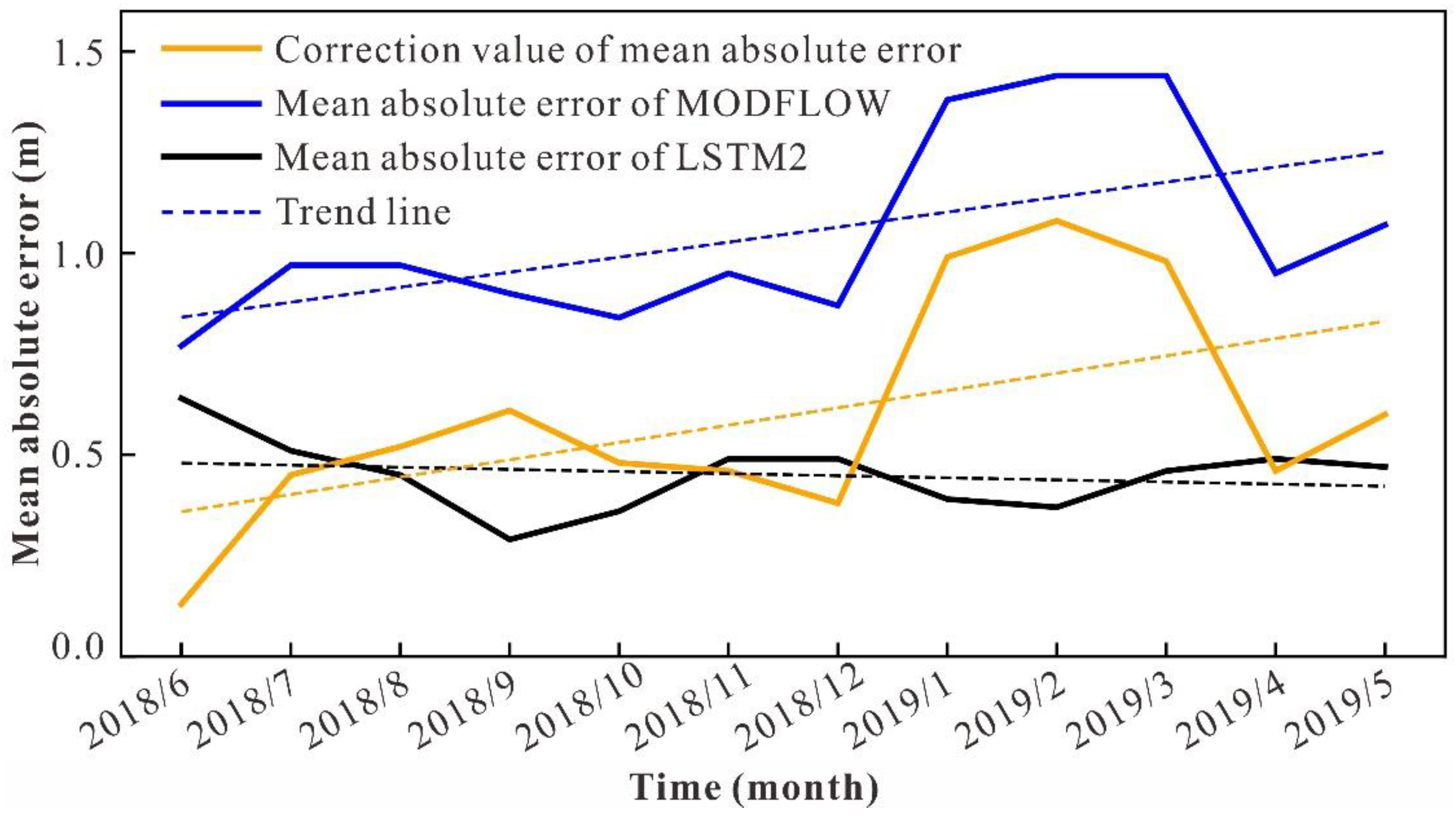
4.1. Temporal Variation Characteristics of the Correction Effect on Accuracy

Based on the analysis in Section 3.3, it is evident that only the LSTM2 model had a significant correction effect on the predicted GWLs via the MODFLOW model. Thus, this section focuses solely on how the correction effect of the LSTM2 model changed over time during the prediction period (June 2018 to May 2019). The correction value of the mean absolute error was used to measure this change characteristic. The calculation steps for this value were as follows: first, the monthly absolute error of the GWLs, predicted by both the MODFLOW model and the LSTM2 model for each well, was calculated; then, the monthly mean absolute error for the 10 wells in the two models was calculated; finally, the correction value of the mean absolute error was obtained by subtracting the monthly mean absolute error of the LSTM2 model from the corresponding month’s mean absolute error of the MODFLOW model (Figure 6). It can be observed that the correction values of the mean absolute error in all months were positive, with the maximum correction value being 1.08 m, the minimum correction value being 0.13 m, and the average correction value being 0.59 m. Additionally, the mean absolute error of the GWLs predicted by the MODFLOW model showed an increasing trend over time, and the curve of the correction value closely followed this trend, with a Pearson correlation coefficient of 0.96. This means that, when the prediction error of the MODFLOW model is large, the correction effect of the LSTM2 model is also large, and when the prediction error is small, the correction effect decreases. As a result, the accuracy of the corrected GWL is relatively stable, with a mean absolute error ranging from 0.29 m to 0.64 m. Reference [18] also supports a similar conclusion that the predictions of machine learning models show relatively stable residuals within the first two years, but exhibit a slight increasing trend over time. This also indicates that the LSTM2 model has the potential to correct long-term GWLs predicted by the MODFLOW model.

4.2. Spatial Variation Characteristics of the Correction Effect on Accuracy

This section also exclusively discusses the LSTM2 model. The RMSE correction value for each well during the prediction period was used to evaluate the relationship between correction effect and spatial location. This value was obtained by subtracting the RMSE of the MODFLOW model’s predicted GWLs for each well from the corresponding RMSE of the LSTM2 model (Figure 7). From Figure 7a, it is evident that most wells located in the middle-lower part of the alluvial fan exhibited larger RMSE values compared to those in the upper-middle part of the MODFLOW model. This is due to the generally larger range of GWL variation in the middle-lower part of the alluvial fan from January 2015 to May 2019, resulting in higher prediction errors at this area in the MODFLOW model. From Figure 7a,b, it can be observed that the spatial distribution pattern between RMSE correction values for different wells and RMSEs of the corresponding wells in MODFLOW was similar. Specifically, larger RMSE correction values corresponded to larger RMSEs in the MODFLOW model. This indicates that, as the prediction error of MODFLOW increases, the correction magnitude of the LSTM2 model also increases, which is consistent with the conclusion in Section 4.1. Therefore, the LSTM2 model generally exhibits a greater correction magnitude for wells in the middle-lower part of the alluvial fan.

4.3. Applicability of Different Methods and Feature Variables for Correcting Predicted GWLs

The difference in correction effects for the GWLs predicted by the MODFLOW model between ensemble learning methods and deep neural networks is significant. In cases of a continuous rise or fall in GWLs, both the RF and XGBoost methods are unable to effectively correct the GWLs predicted by the MODFLOW model. The reason includes two aspects. Firstly, the continuous rise or fall of GWLs causes the future GWLs, which need to be predicted, to exceed the range of historical GWLs used for training the model. However, both models rely on the relationship between feature variables and the target variable in the training data, which may not hold true outside the data range. Secondly, both models are based on multiple decision trees for prediction, and decision trees typically provide local average predictions at the leaf nodes. However, when the prediction falls outside the range of the training data, there are no leaf nodes to refer to, making it difficult for the model to make accurate predictions. As a result, these two algorithms are not suitable for correcting predicted GWL in the aforementioned scenarios. However, when the predicted GWLs do not exceed the range of the training set, these algorithms may have some corrective effect.

Compared to ensemble learning algorithms, the LSTM algorithm can capture long-term trends and short-term seasonal fluctuations in GWLs, demonstrating good extrapolation performance (the prediction set exceeding the range of the training set). This is because of its “gate mechanism” structure (consisting of memory cells and gate units), which allows it to better capture and remember long-term dependencies in the data. By selectively forgetting and updating information, LSTM can effectively retain useful information over longer time ranges. These characteristics enable it to better grasp the long-term and short-term patterns in the data, and to make relatively accurate predictions for data beyond the training set. Therefore, the LSTM algorithm can be used for correcting GWLs predicted by the MODFLOW model in complex scenarios.

Regarding the selection of feature variables, it is evident that using additional feature variables such as precipitation, extraction, and replenishment along with the predicted GWLs from MODFLOW leads to better correction compared to using only the predicted GWLs from MODFLOW. This may be because these extra variables help the model to better understand the system’s complexity and variations, thus improving the correction effect.

5. Conclusions

In this study, the correction effects of two ensemble algorithms, RF and XGBoost, as well as a deep neural network with LSTM architecture, were compared under different feature variables for the predicted GWLs from the MODFLOW model. The 10 wells located at different sections of the Hutuo River alluvial fan, including the upper, middle, and lower areas, were chosen to assess the correction effects. The primary conclusions are as follows.

(1) All tested algorithms performed well in the simulation period (the training and validation period). The average NSE values for the RF1, RF2, XGBoost1, XGBoost2, LSTM1, and LSTM2 models were 0.81, 0.88, 0.84, 0.87, 0.73, and 0.89, respectively. However, during the prediction period, the RF1, RF2, XGBoost1, and XGBoost2 models did not effectively correct the GWLs predicted by MODFLOW for most wells, as the prediction dataset exceeded the range of the training dataset. All four types of models demonstrated that PR could be corrected for less than 40% of the wells, and RMSE could be corrected for less than 20% of the wells. In contrast, the LSTM algorithm showed better correction performance than the ensemble algorithms during the same period. Specifically, the LSTM1 model could correct the PR metric for 60% of the wells, with a maximum increase of 0.35 and a minimum increase of 0.01. It also corrected the RMSE metric for 50% of the wells, with a maximum decrease of 0.71 m and a minimum decrease of 0.12 m. Furthermore, the LSTM2 model, which incorporated additional source–sink feature variables based on MODFLOW’s predicted GWLs, was able to improve the PR for 80% of the wells, with a maximum increase of 1.26 and a minimum increase of 0.02, and to reduce the RMSE for 100% of the wells, with a maximum decrease of 1.59 m and a minimum decrease of 0.17 m.

(2) During the simulation period, all models generally performed better than the MODFLOW model in terms of capturing long-term GWL trends and short-term seasonal fluctuations. However, during the prediction period, the RF and XGBoost algorithms showed a significant decline in their ability to capture the dynamic behavior of GWLs. In contrast, the LSTM algorithm still performed well, but the LSTM1 model performed worse than MODFLOW. Only the LSTM2 model showed a substantial improvement compared to MODFLOW. Therefore, ensemble algorithms such as RF and XGBoost are not suitable for correcting extrapolation predictions in scenarios of continuous rising or falling of GWL. In contrast, the LSTM algorithm is suitable for correcting predicted GWL from MODFLOW in complex situations. Additionally, in terms of correction, models that incorporate source–sink feature variables perform better than models that solely rely on the GWLs predicted by MODFLOW.

(3) Throughout the prediction period, the LSTM2 model consistently produced positive correction values of the mean absolute error. The maximum correction value was 1.08 m, the minimum was 0.13 m, and the mean correction value was 0.59 m. Furthermore, there was a positive correlation between the correction magnitude of the LSTM2 model and the prediction error of the MODFLOW model, indicating that the greater the prediction error of the MODFLOW model, the larger the correction magnitude of the LSTM2 model. This pattern also held true spatially, and the LSTM2 model generally exhibited a greater correction magnitude for wells located in the middle-lower part of the alluvial fan.

References

1. Moghaddam, H.K.; Moghaddam, H.K.; Kivi, Z.R.; Bahreinimotlagh, M.; Alizadeh, M.J. Developing comparative mathematic models, BN and ANN for forecasting of groundwater levels. Groundw. Sustain. Dev. 2019, 9, 100237. [Google Scholar] [CrossRef]
2. Long, D.; Yang, W.; Scanlon, B.R.; Zhao, J.; Liu, D.; Burek, P.; Pan, Y.; You, L.; Wada, Y. South-to-North Water Diversion stabilizing Beijing’s groundwater levels. Nat. Commun. 2020, 11, 3665. [Google Scholar] [CrossRef]
3. Dangar, S.; Asoka, A.; Mishra, V. Causes and implications of groundwater depletion in India: A review. J. Hydrol. 2021, 596, 126103. [Google Scholar] [CrossRef]
4. Taylor, R.G.; Scanlon, B.; Doell, P.; Rodell, M.; van Beek, R.; Wada, Y.; Longuevergne, L.; Leblanc, M.; Famiglietti, J.S.; Edmunds, M.; et al. Ground water and climate change. Nat. Clim. Change 2013, 3, 322–329. [Google Scholar] [CrossRef]
5. Famiglietti, J.S. The global groundwater crisis. Nat. Clim. Change 2014, 4, 945–948. [Google Scholar] [CrossRef]
6. Richey, A.S.; Thomas, B.F.; Lo, M.-H.; Famiglietti, J.S.; Swenson, S.; Rodell, M. Uncertainty in global groundwater storage estimates in a Total Groundwater Stress framework. Water Resour. Res. 2015, 51, 5198–5216. [Google Scholar] [CrossRef]
7. Hellwig, J.; de Graaf, I.E.M.; Weiler, M.; Stahl, K. Large-Scale Assessment of Delayed Groundwater Responses to Drought. Water Resour. Res. 2020, 56, e2019WR025441. [Google Scholar] [CrossRef]
8. Doell, P.; Mueller Schmied, H.; Schuh, C.; Portmann, F.T.; Eicker, A. Global-scale assessment of groundwater depletion and related groundwater abstractions: Combining hydrological modeling with information from well observations and GRACE satellites. Water Resour. Res. 2014, 50, 5698–5720. [Google Scholar] [CrossRef]
9. Neuman, S.P.; Wierenga, P.J. A Comprehensive Strategy of Hydrogeologic Modeling and Uncertainty Analysis for Nuclear Facilities and Sites; NUREG/CR-6805, Prepared for US Nuclear Regulatory Commission; United States Environmental Protection Agency: Washington, DC, USA, 2003; Volume 309.
10. Cooley, R.L. A Theory for Modeling Ground-Water Flow in Heterogeneous Media; U.S. Geological Survey Professional Paper; U.S. Geological Survey: Reston, VA, USA, 2004; Volume 1679, p. 220.
11. Doherty, J.; Christensen, S. Use of paired simple and complex models to reduce predictive bias and quantify uncertainty. Water Resour. Res. 2011, 47, W12534. [Google Scholar] [CrossRef]
12. Refsgaard, J.C.; van der Sluijs, J.P.; Brown, J.; van der Keur, P. A framework for dealing with uncertainty due to model structure error. Adv. Water Resour. 2006, 29, 1586–1597. [Google Scholar] [CrossRef]
13. Hunt, R.J.; Welter, D.E. Taking Account of “Unknown Unknowns”. Ground Water 2010, 48, 477. [Google Scholar] [CrossRef]
14. Hill, M.C.; Tiedeman, C.R. Effective Groundwater Model Calibration: With Analysis of Data, Sensitivities, Predictions, and Uncertainty; Center for Integrated Data Analytics: Middleton, WI, USA, 2007.
15. Liu, Y.; Gupta, H.V. Uncertainty in hydrologic modeling: Toward an integrated data assimilation framework. Water Resour. Res. 2007, 43, W07401. [Google Scholar] [CrossRef]
16. Vrugt, J.A.; ter Braak, C.J.F.; Clark, M.P.; Hyman, J.M.; Robinson, B.A. Treatment of input uncertainty in hydrologic modeling: Doing hydrology backward with Markov chain Monte Carlo simulation. Water Resour. Res. 2008, 44, W00B09. [Google Scholar] [CrossRef]
17. Xu, T.; Valocchi, A.J.; Choi, J.; Amir, E. Use of Machine Learning Methods to Reduce Predictive Error of Groundwater Models. Groundwater 2014, 52, 448–460. [Google Scholar] [CrossRef] [PubMed]
18. Demissie, Y.K.; Valocchi, A.J.; Minsker, B.S.; Bailey, B.A. Integrating a calibrated groundwater flow model with error-correcting data-driven models to improve predictions. J. Hydrol. 2009, 364, 257–271. [Google Scholar] [CrossRef]
19. Reichstein, M.; Camps-Valls, G.; Stevens, B.; Jung, M.; Denzler, J.; Carvalhais, N.; Prabhat, F. Deep learning and process understanding for data-driven Earth system science. Nature 2019, 566, 195–204. [Google Scholar] [CrossRef] [PubMed]
20. Jiang, Z.; Yang, S.; Liu, Z.; Xu, Y.; Shen, T.; Qi, S.; Pang, Q.; Xu, J.; Liu, F.; Xu, T. Can ensemble machine learning be used to predict the groundwater level dynamics of farmland under future climate: A 10-year study on Huaibei Plain. Environ. Sci. Pollut. Res. 2022, 29, 44653–44667. [Google Scholar] [CrossRef]
21. Wu, M.; Feng, Q.; Wen, X.; Yin, Z.; Yang, L.; Sheng, D. Deterministic Analysis and Uncertainty Analysis of Ensemble Forecasting Model Based on Variational Mode Decomposition for Estimation of Monthly Groundwater Level. Water 2021, 13, 139. [Google Scholar] [CrossRef]
22. Quoc Bao, P.; Kumar, M.; Di Nunno, F.; Elbeltagi, A.; Granata, F.; Islam, A.R.M.T.; Talukdar, S.; Nguyen, X.C.; Ahmed, A.N.; Duong Tran, A. Groundwater level prediction using machine learning algorithms in a drought-prone area. Neural Comput. Appl. 2022, 34, 10751–10773. [Google Scholar] [CrossRef]
23. Sun, J.; Hu, L.; Li, D.; Sun, K.; Yang, Z. Data-driven models for accurate groundwater level prediction and their practical significance in groundwater management. J. Hydrol. 2022, 608, 127630. [Google Scholar] [CrossRef]
24. Zhang, X.; He, J.; He, B.; Sun, J. Assessment, formation mechanism, and different source contributions of dissolved salt pollution in the shallow groundwater of Hutuo River alluvial-pluvial fan in the North China Plain. Environ. Sci. Pollut. Res. 2019, 26, 35742–35756. [Google Scholar] [CrossRef] [PubMed]
25. Zhang, P.; Hao, Q.; Fei, Y.; Li, Y.; Zhu, Y.; Li, J. Simulation-optimization model for groundwater replenishment from the river: A case study in the Hutuo River alluvial fan, China. Water Supply 2022, 22, 6994–7005. [Google Scholar] [CrossRef]
26. Harbaugh, A.W. MODFLOW-2005, The US Geological Survey Modular Groundwater Model-the Groundwater Flow Process; U.S. Geological Survey: Reston, VA, USA, 2005.
27. Sahin, E.K.; Colkesen, I.; Kavzoglu, T. A comparative assessment of canonical correlation forest, random forest, rotation forest and logistic regression methods for landslide susceptibility mapping. Geocarto Int. 2020, 35, 341–363. [Google Scholar] [CrossRef]
28. Groemping, U. Variable Importance Assessment in Regression: Linear Regression versus Random Forest. Am. Stat. 2009, 63, 308–319. [Google Scholar] [CrossRef]
29. Breiman, L. Random forests. Mach. Learn. 2001, 45, 5–32. [Google Scholar] [CrossRef]
30. Belgiu, M.; Dragut, L. Random forest in remote sensing: A review of applications and future directions. ISPRS J. Photogramm. 2016, 114, 24–31. [Google Scholar] [CrossRef]
31. Baker, H.; Hallowell, M.R.; Tixier, A.J.P. AI-based prediction of independent construction safety outcomes from universal attributes. Autom. Constr. 2020, 118, 103146. [Google Scholar] [CrossRef]
32. Barzegar, R.; Razzagh, S.; Quilty, J.; Adamowski, J.; Pour, H.K.; Booij, M.J. Improving GALDIT-based groundwater vulnerability predictive mapping using coupled resampling algorithms and machine learning models. J. Hydrol. 2021, 598, 126370. [Google Scholar] [CrossRef]
33. Kavzoglu, T.; Teke, A. Predictive Performances of Ensemble Machine Learning Algorithms in Landslide Susceptibility Mapping Using Random Forest, Extreme Gradient Boosting (XGBoost) and Natural Gradient Boosting (NGBoost). Arab. J. Sci. Eng. 2022, 47, 7367–7385. [Google Scholar] [CrossRef]
34. Naghibi, S.A.; Ahmadi, K.; Daneshi, A. Application of Support Vector Machine, Random Forest, and Genetic Algorithm Optimized Random Forest Models in Groundwater Potential Mapping. Water Resour. Manag. 2017, 31, 2761–2775. [Google Scholar] [CrossRef]
35. Rahmati, O.; Pourghasemi, H.R.; Melesse, A.M. Application of GIS-based data driven random forest and maximum entropy models for groundwater potential mapping: A case study at Mehran Region, Iran. Catena 2016, 137, 360–372. [Google Scholar] [CrossRef]
36. Choubin, B.; Rahmati, O. Water Engineering Modeling and Mathematic Tools; Elsevier: Amsterdam, The Netherlands, 2021. [Google Scholar]
37. Chen, T.; Guestrin, C. XGBoost: A Scalable Tree Boosting System. In Proceedings of the 22nd ACM SIGKDD International Conference on Knowledge Discovery and Data Mining (KDD), San Francisco, CA, USA, 13–17 August 2016; pp. 785–794. [Google Scholar]
38. Jing, H.; He, X.; Tian, Y.; Lancia, M.; Cao, G.; Crivellari, A.; Guo, Z.; Zheng, C. Comp arison and interpretation of data-driven models for simulating site-specific human-impacted groundwater dynamics in the North China Plain. J. Hydrol. 2023, 616, 128751. [Google Scholar] [CrossRef]
39. Li, L.; Qiao, J.; Yu, G.; Wang, L.; Li, H.-Y.; Liao, C.; Zhu, Z. Interpretable tree-based ensemble model for predicting beach water quality. Water Res. 2022, 211, 118078. [Google Scholar] [CrossRef]
40. Hochreiter, S.; Schmidhuber, J. Long short-term memory. Neural Comput. 1997, 9, 1735–1780. [Google Scholar] [CrossRef] [PubMed]
41. Greff, K.; Srivastava, R.K.; Koutnik, J.; Steunebrink, B.R.; Schmidhuber, J. LSTM: A Search Space Odyssey. IEEE Trans. Neural Netw. Learn. Syst. 2017, 28, 2222–2232. [Google Scholar] [CrossRef]
42. Bowes, B.D.; Sadler, J.M.; Morsy, M.M.; Behl, M.; Goodall, J.L. Forecasting Groundwater Table in a Flood Prone Coastal City with Long Short-term Memory and Recurrent Neural Networks. Water 2019, 11, 1098. [Google Scholar] [CrossRef]
43. Guo, X.; Gui, X.; Xiong, H.; Hu, X.; Li, Y.; Cui, H.; Qiu, Y.; Ma, C. Critical role of climate factors for groundwater potential mapping in arid regions: Insights from random forest, XGBoost, and LightGBM algorithms. J. Hydrol. 2023, 621, 129599. [Google Scholar] [CrossRef]
44. Goodfellow, I.; Bengio, Y.; Courville, A. Deep Learning; The MIT Press: Cambridge, MA, USA, 2016. [Google Scholar]
45. Yang, S.; Yang, D.; Chen, J.; Zhao, B. Real-time reservoir operation using recurrent neural networks and inflow forecast from a distributed hydrological model. J. Hydrol. 2019, 579, 124229. [Google Scholar] [CrossRef]
46. Moriasi, D.N.; Arnold, J.G.; Liew, M.W.V.; Bingner, R.L.; Harmel, R.D.; Veith, T.L. Model Evaluation Guidelines for Systematic Quantification of Accuracy in Watershed Simulations. Trans. ASABE 2007, 50, 885–900. [Google Scholar] [CrossRef]
47. Yin, W.; Fan, Z.; Tangdamrongsub, N.; Hu, L.; Zhang, M. Comparison of physical and data-driven models to forecast groundwater level changes with the inclusion of GRACE—A case study over the state of Victoria, Australia. J. Hydrol. 2021, 602, 126735. [Google Scholar] [CrossRef]
48. Zhang, M.; Hu, L.; Yao, L.; Yin, W. Surrogate Models for Sub-Region Groundwater Management in the Beijing Plain, China. Water 2017, 9, 766. [Google Scholar] [CrossRef]
49. Zhang, M.; Hu, L.; Yao, L.; Yin, W. Numerical studies on the influences of the South-to-North Water Transfer Project on groundwater level changes in the Beijing Plain, China. Hydrol. Process. 2018, 32, 1858–1873. [Google Scholar] [CrossRef]
Figure 1. Location of the study area and the groundwater monitoring wells.
Sustainability 16 00653 g001
Figure 2. Flowchart of this study.
Sustainability 16 00653 g002
Figure 3. Scatter plot of GWLs predicted by MODFLOW and observed values. (a) Observed and predicted GWLs for 39 wells; (b) Taylor diagram for 39 wells.
Sustainability 16 00653 g003
Figure 4. Taylor diagram of PR and RMSE for 10 wells at prediction periods based on different models. Note: (a) describes wells numbered 1 and 2; (b) describes wells numbered 3 and 4; (c) describes wells numbered 5 and 6; (d) describes wells numbered 7 and 8; and (e) describes wells numbered 9 and 10. The well numbers in parentheses indicate negative PR values, with the absolute value used instead.
Sustainability 16 00653 g004
Figure 5. Comparison of simulated dynamic GWL curves for 3 wells based on different models. Note: Simulation period includes training period and validation period; No. 2, No. 6, and No. 10 represent wells numbered 2, 6, and 10, respectively; (a,d,g) represent the dynamic GWL curves plotted by the RF1 and RF2 models; (b,e,h) represent the dynamic GWL curves plotted by the XGBoost1 and XGBoost2 models; and (c,f,i) represent the dynamic GWL curves plotted by the LSTM1 and LSTM2 models.
Sustainability 16 00653 g005
Figure 6. Variation curves of correction value of mean absolute error over time for LSTM2 model during the prediction period. Note: Correction value of mean absolute error = mean absolute error of MODFLOW model − mean absolute error of LSTM2 model.
Sustainability 16 00653 g006
Figure 7. Spatial distribution of RMSEs and RMSE correction values for 10 wells during the prediction period. Note: (a) RMSE of the GWLs predicted by the MODFLOW model; (b) RMSE correction value; RMSE correction value = RMSE of MODFLOW model − RMSE of LSTM2 model. Numbers 1 to 10 correspond to wells numbered 1 to 10, respectively; “1/5.0” represents the well numbered 1 and the overall range of GWL variation for this well from January 2015 to May 2019.
Sustainability 16 00653 g007