Greenhouse Gas Emissions Performance of Electric, Hydrogen and Fossil-Fuelled Freight Trucks with Uncertainty Estimates Using a Probabilistic Life-Cycle Assessment (pLCA)

Abstract

This research conducted a probabilistic life-cycle assessment (pLCA) into the greenhouse gas (GHG) emissions performance of nine combinations of truck size and powertrain technology for a recent past and a future (largely decarbonised) situation in Australia. This study finds that the relative and absolute life-cycle GHG emissions performance strongly depends on the vehicle class, powertrain and year of assessment. Life-cycle emission factor distributions vary substantially in their magnitude, range and shape. Diesel trucks had lower life-cycle GHG emissions in 2019 than electric trucks (battery, hydrogen fuel cell), mainly due to the high carbon-emission intensity of the Australian electricity grid (mainly coal) and hydrogen production (mainly through steam–methane reforming). The picture is, however, very different for a more decarbonised situation, where battery electric trucks, in particular, provide deep reductions (about 75–85%) in life-cycle GHG emissions. Fuel-cell electric (hydrogen) trucks also provide substantial reductions (about 50–70%), but not as deep as those for battery electric trucks. Moreover, hydrogen trucks exhibit the largest uncertainty in emissions performance, which reflects the uncertainty and general lack of information for this technology. They therefore carry an elevated risk of not achieving the expected emission reductions. Battery electric trucks show the smallest (absolute) uncertainty, which suggests that these trucks are expected to deliver the deepest and most robust emission reductions. Operational emissions (on-road driving and vehicle maintenance combined) dominate life-cycle emissions for all vehicle classes. Vehicle manufacturing and upstream emissions make a relatively small contribution to life-cycle emissions from diesel trucks (<5% each), but these are important aspects for electric trucks (5% to 30%).

1. Introduction

Road transport contributes significantly to total greenhouse gas emissions, and this contribution is growing. In Australia, the contribution is currently 16% [1], but in the EU, it is already the largest source, contributing 30% to total greenhouse gas (GHG) emissions [2]. Unlike the other sectors, the transport sector proves particularly resistant to decoupling from economic growth [3], which is why addressing its relatively poor GHG emissions performance needs to be given special priority. Despite their small share of total stravel, heavy-duty vehicles are typically responsible for about 25% of total road transport emissions, and their relative contribution is growing [2,4,5].

1.1. Life-Cycle Analysis

It is increasingly accepted that life-cycle assessment (LCA) is required for the adequate estimation of GHG emissions from road transport, which is currently shifting from fossil-fuelled to electric and hydrogen-powered transport [1]. LCA can examine different types of environmental impacts [6,7]. LCA quantifies the environmental impacts of a product’s manufacture, operational use and end of life using holistic system boundaries [8,9,10].

LCA studies are often restricted in scope given the complexity and resources required to conduct this type of study (it is noted that some ISO standards have flexible definitions in relation to global warming impacts e.g., [9,10,11]). A particular challenge is that LCA quantifies impacts for a system that is intrinsically complex, location-specific and that varies in time and over time (trends). In addition, LCA often deals with incomplete information due to data gaps, restricted access and confidentiality issues.

As a consequence, it is critical that the uncertainty in the study results is quantified, and that these results are regularly updated, refined, expanded and improved [12,13,14]. Despite certain limitations regarding its accuracy, LCA appears to be the best way to make informed decisions regarding cost-effective GHG emissions reductions e.g., [15]. Probabilistic LCA (pLCA) is a particularly cost-effective, powerful and flexible approach to LCA. pLCA is designed to focus on available data and to use expert judgement to address gaps (e.g., [16]). Moreover, it aims to rapidly absorb continuous improvements in input data and new information, thereby generally reducing the uncertainty in the updated study results.

1.2. Background and Purpose of This Study

This paper extends a previous probabilistic LCA (pLCA) study into the GHG emissions performance of Australian passenger vehicles [17] to Australian freight vehicles (trucks). A more detailed introduction and discussion of LCA studies is provided in Smit and Kennedy [17] and will not be repeated here. A number of inputs from this previous study [17] will be re-used in this paper. Where this is the case, reference is made to the previous publication.

Compared with passenger vehicles, a life-cycle assessment for trucks is more challenging due to the wide range of possible vehicle configurations and associated vehicle uses, as well as the generally larger gaps in available data and information. In this respect, the application of a probabilistic life-cycle method is particularly useful, since it explicitly considers and reflects this increased variability and uncertainty in the final life-cycle results.

This study will examine the life-cycle GHG emissions performance of three truck sizes, three powertrains (internal combustion engine, battery electric and hydrogen fuel cell) and for a recent past and a future (largely decarbonised) situation. Wherever possible, quantitative data will be used, either of empirical origin or from reliable and proven software packages, supplemented with information from relevant scientific literature. In the absence of quantitative data, expert judgement will be exercised.

A range of fundamental and relevant input variables will be considered, including (but not limited to) vehicle lifetime, accumulated mileage, size and durability of battery and fuel-cell systems; emission intensities of electricity generation and hydrogen production; battery charging losses; hydrogen distribution losses and energy requirements of on-road driving. Interdependencies between variables will be accounted for in the calculations. For instance, the impact of variable vehicle (tare) mass on operational emissions is modelled in the simulation with correction functions. Future improvements (and their associated uncertainty) will be discussed and explicitly modelled.

The focus is on freight vehicles in the Australian on-road fleet, which have a few unique characteristics such as lifetime mileage compared with other major jurisdictions, as will be discussed later. There are a few additional differences with other LCA studies. For instance, this study is more comprehensive than studies that have not included upstream impacts e.g., [18], and it focuses on future fuels (electricity, hydrogen) rather than alternative fossil fuels such as natural gas e.g., [19]. A comparison will be made with international studies [20] in Section 4.3.

2. Materials and Methods

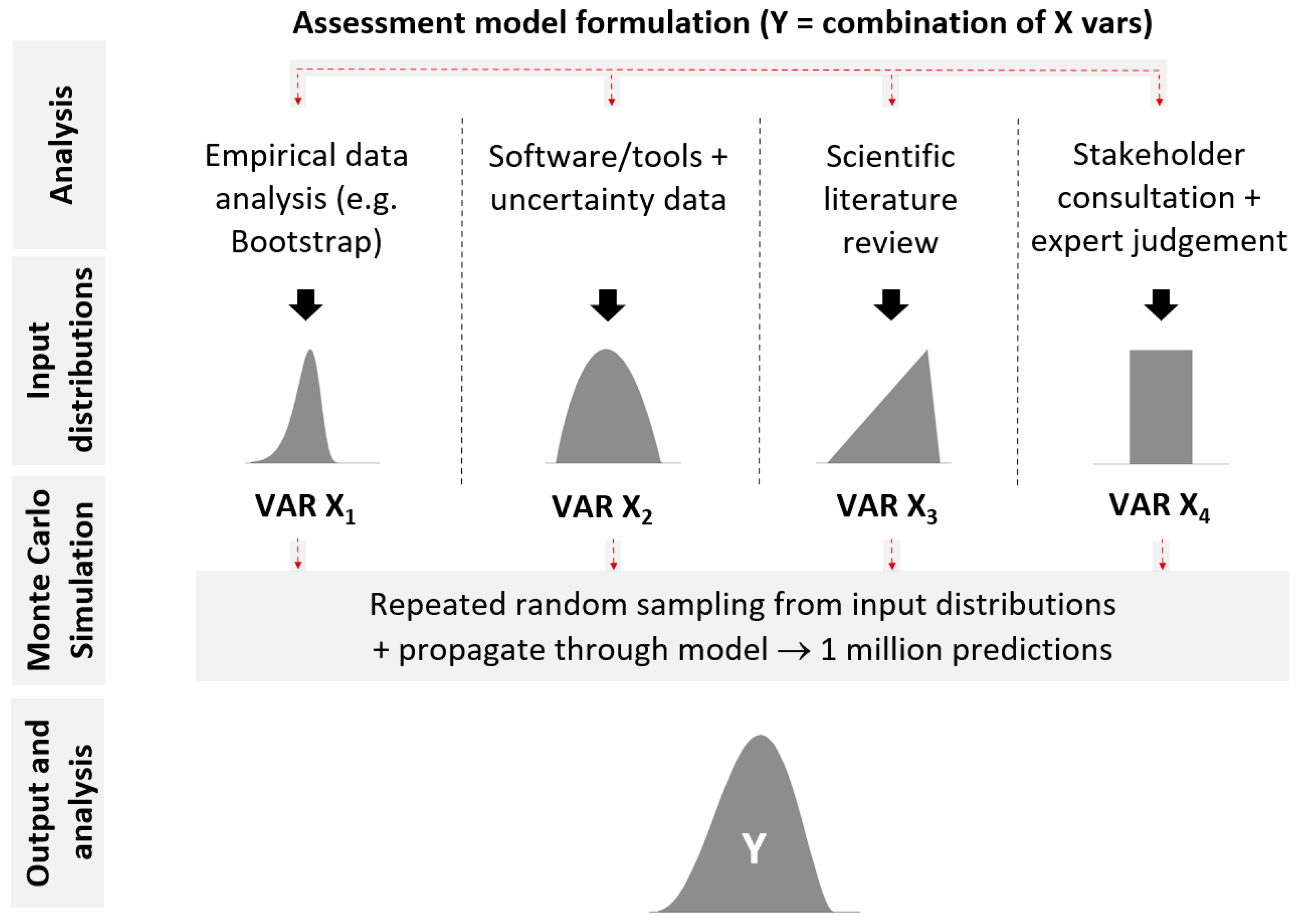
2.1. Probabilistic LCA (pLCA)

A probabilistic LCA (pLCA) approach quantifies uncertainty and variability in model outputs and estimates non-linear interactions [21]. The method provides an estimate of robustness and provides insight into which LCA aspects are the most uncertain and could benefit most from further research e.g., [16]. This assists with the cost-effective use of available resources to further improve, refine and expand the LCA results. Figure 1 shows a flow diagram that visualises the pLCA approach used in this study.

The process starts with a mathematical formulation of the life-cycle assessment model; in this study, the response variable Y quantifies the greenhouse gas emissions performance (Section 2.2), and the predictor variables X₁, X₂, …, X_n (Section 2.3) collectively explain and quantify the magnitude of and the variability and uncertainty in the response variable. In the analysis phase, a range of methods are used to define the input distributions for each predictor variable, where the choice of method(s) is guided by the available information and data (Section 2.3 and Section 3). The probabilistic definition of input variables is based on the statistical analysis of empirical data, software simulation, results from peer-reviewed scientific studies or expert judgement wherever available and in this order of preference.

In a Monte Carlo simulation (Section 2.3), random samples are taken from input distributions (typically a hundred thousand to a million times) and propagated through the LCA model to create probability output distributions. This way, it is not only the expected values that are estimated, but also the associated variability and uncertainty. The process is a mathematical analogue of an experiment, which is repeated many times to provide an accurate description of the variability and uncertainty in the output estimate Y. The final step is then an analysis of the output data and its comparison with other studies (Section 4).

2.2. Model Definition

The assessment variable, or functional unit, in this study is the life-cycle greenhouse gas (GHG) emission factor. This factor standardises the environmental impact, specifically expressed as the quantity of GHG emissions per kilometre driven by a vehicle, denoted as CO₂-e/vehicle.km. The computation of carbon dioxide equivalent (CO₂-e) emissions involves multiplying the emissions of a particular greenhouse gas by its global-warming potential (GWP) and aggregating these emissions.

All pertinent aspects of GHG emissions throughout the vehicle’s life cycle are taken into account, including: (1) production of the vehicle (manufacturing of non-battery components and manufacturing of the battery and fuel-cell system); (2) production of (fossil) fuels for internal combustion engine vehicles (ICEVs) (extraction, transport and fuel refining); (3) production of electricity for battery electric vehicles (BEVs) (extraction and transport of fossil fuels, electricity generation, electricity distribution losses and power-generation infrastructure); (4) production of hydrogen for fuel-cell electric vehicles (FCEVs) (extraction and transport of fossil fuels, hydrogen production, compression, distribution, refuelling losses and leakage); (5) on-road operation of the vehicle (ICEV fossil-fuel use, BEV energy use, BEV battery charging losses, FCEV hydrogen use and leakage losses and vehicle maintenance); and (6) disposal and recycling of the vehicle at the end of its life.

For clarity and readability of the paper, two different aspects of the “production of energy and fuels” are allocated to different LCA aspects, depending on the vehicle technology. For ICEVs, the production of fossil fuels (extraction, transport, fuel refining and distribution) is reflected in the upstream LCA aspect. For BEVs, the emission intensity of electricity generation is included in the on-road operation aspect (indirect energy use), whereas the energy input for electricity generation (extraction and transport of fossil fuels and use of renewables) is incorporated into the upstream LCA aspect. For FCEVs, the emission intensity of hydrogen production and distribution (indirect energy use) is included in the on-road operation aspect, whereas the energy input for hydrogen production (extraction and transport of natural gas and water) is incorporated into the upstream LCA aspect.

The life-cycle GHG emission factors, e_ICEV, e_BEV and e_FCEV, are computed using three basic additive models and sub-models (if applicable), as shown in

Table 1. pLCA model structure and definition.

Notation	Description and Units	Time Variable
Mx	lifetime mileage for technology x (x = ICEV, BEV, FCEV) (km)	No (S.3.1)
ΓBAT	battery replacement factor (−)	Yes (S.3.1)
ΓFCL	fuel-cell replacement factor (−)	Yes (S.3.1)
Mx	vehicle tare mass for technology x (x = ICEV, BEV, FCEV) (kg)	No (S.3.2)
MBAT	battery mass for BEV or FCEV (kg)	No (S.3.2)
MFCL	fuel-cell mass (kg)	No (S.3.2)
θBAT	battery capacity (kWh)	Yes (S.3.2)
ρFCL	fuel-cell rated power (kW)	Yes (S.3.2)
ωelec (1)	GHG emission-intensity electricity generation (g CO2-e/kWh generated)	Yes (S.3.3)
ηb	battery recharging efficiency (−)	Yes (S.3.3)
ηg	grid transmission efficiency (−)	Yes (S.3.3)
ωH2,P	GHG emission-intensity hydrogen production (g CO2-e/g fuel) for production pathway P	Yes (S.3.4)
σelec	GHG emission-intensity electricity infrastructure (g CO2-e/kWh generated)	Yes (S.3.5)
ηh	hydrogen distribution efficiency (−)	Yes (S.3.4)
ηr	hydrogen refuelling efficiency (−)	Yes (S.3.4)
σH2,P	GHG emission-intensity H2 production infrastructure (g CO2-e/g fuel) production pathway P	Yes (S.3.5)
ϕelec (2)	GHG emission-intensity upstream fuels for electricity generation (g CO2-e/kWh consumed)	Yes (S.3.5)
ϕH2,p (2)	GHG emission-intensity upstream H2 production (g CO2-e/g fuel) for production pathway P	Yes (S.3.5)
φv,ICEV	GHG emission-intensity ICEV production (kg CO2-e/kg vehicle)	Yes (S.3.6)
φv,BEV	GHG emission-intensity BEV production without battery (kg CO2-e/kg vehicle)	Yes (S.3.6)
φv,FCEV	GHG emission-intensity FCEV production without battery/fuel cell (kg CO2-e/kg vehicle)	Yes (S.3.6)
φBAT	GHG emission-intensity battery production (kg CO2-e/kWh battery capacity)	Yes (S.3.6)
φFCL	GHG emission-intensity fuel-cell production (kg CO2-e/kW fuel-cell-rated power)	Yes (S.3.6)
ε	real-world electricity consumption BEV (kWh/km)	Yes (S.3.7)
H	real-world hydrogen consumption FCEV (g/km)	Yes (S.3.7)

⁽¹⁾ Direct emissions due to the activity; ⁽²⁾ Indirect emissions from upstream activities (extraction, production, etc.).

. In Equations (1)–(3), e_i,j is used to represent a GHG emission factor (CO₂-e/km) for a life-cycle aspect i and vehicle type j. This research focuses on assessing the fleet’s average impact. Therefore, fleet-averaged input data are generally used, such as mean vehicle mass and the associated probability distribution of this mean value. While the pLCA method can be employed for individual vehicles if desired, this falls outside the scope of this study. Such an analysis would require the utilization of vehicle-specific input data instead of the aggregated data used for fleet averages.

2.3. Developing Input Distributions

The model variables in Equations (1)–(3) are defined as parametric distributions, which represent the probabilities of all possible values in the sample space [21]. A probability model is mathematically defined as a probability distribution in the form of either a probability density function (PDF) or cumulative distribution function (CDF) with associated parameters (minimum, maximum, scale, shape, etc.).

Whenever possible, quantitative data were employed to construct input distributions, complemented by information sourced from the existing scientific literature. Quantitative data encompassed empirical data, reported findings in the scientific literature, or output from relevant vehicle emissions software. Various statistical techniques, including Monte Carlo simulation, bootstrap analysis, and parametric distribution fitting, were employed in the development of these input distributions.

In cases where empirical input data were accessible for aspects of the life-cycle assessment (LCA), the data were either directly utilized as sampling distributions or were transformed into sampling distributions through bootstrap analyses. The statistical bootstrap technique [22] was employed to generate resampled input distributions for a targeted statistic, such as the mean or median. This simulation method approximates an asymptotically accurate sampling distribution by iteratively resampling with replacement from the original data and calculating the desired statistic [23]. Standard errors and confidence intervals were derived from these (non-symmetric) distributions. The boot R package, as developed by Ripley [24], was employed to execute the bootstrap analysis.

eICEV = evehicle,ICEV + einfra,ICEV + efuel,ICEV + eroad,ICEV + edisposal,ICEV	(1)
evehicle,ICEV = wICEV φv,ICEV/MICEV
eBEV = evehicle,BEV + einfra,BEV + efuel,BEV + eroad,BEV + edisposal,BEV	(2)
evehicle,BEV = ((MBEV − MBAT) φv,BEV + (ΓBAT φBAT θBAT))/MBEV
einfra,BEV = ε σelec/(ηg ηb)
efuel,BEV = ε ϕelec/ηb
eroad,BEV = ε ωelec/(ηg ηb)
eFCEV = evehicle,FCEV + einfra, FCEV + efuel,FCEV + eroad,FCEV + edisposal, FCEV	(3)
evehicle,FCEV = ((MFCEV − MBAT − MFCL) φv,FCEV + (ΓBAT φBAT θBAT) + (ΓFCL φFCL ρFCL))/MFCEV
einfra,FCEV = H σH2,p/ηh
efuel,FCEV = H ϕH2,p/ηh
eroad,FCEV = H ωH2,p/ηr

Truncated parametric distributions were fitted to the sampling distributions by maximum likelihood. The following candidates [25,26,27] were included: Uniform (U: a, b), Triangular (T: a, b, c), Normal (N: m, s), Lognormal (L: m, s), Weibull (W: s, s), Gamma (G: s, r), Exponential (E: s), non-standard beta distribution (B: s, s), the location-scale t-distribution (O: m, s, df) and the skew t-distribution (S: m, s, a, df). The Dirac Delta function (D: m) was used to describe a constant value. Appendix A provides further information for the distributions. The “truncdist” R package [28] was deployed to apply truncations to the fitted distributions (setting a lower limit (a) and an upper limit (b)). The plausible range in the input data is defined as the 99.7% confidence interval (equivalent to ±3 SD in a normal distribution), which prevents the use of unrealistic values in the pLCA. In the optimised fitting process, the R packages “fitdistr” and “fitdistrplus” [29], “extraDistr” [26], “sn” [30] and “truncdist” were used.

The identification of the most suitable theoretical distribution involved a comprehensive comparison of all the fitted parametric distributions with the input values from the sampling data. This evaluation was conducted visually using quantile–quantile (QQ) plots for all the fitted distributions and by employing the Cramer–Von Mises test [31], a statistical method for assessing the goodness-of-fit. QQ plots, a graphical tool, enable the comparison of quantiles between two probability distributions.

In instances where there were insufficient quantitative input data for certain model aspects, two simplified distributions [25] were utilised, and parameters were estimated based on a literature review. The uniform (rectangular) distribution, defined by a lower limit (a) and an upper limit (b) within a plausible range (U: a, b), signifies equal probability between these endpoints. This distribution is suitable when information is only available for the lower and upper limit values [32]. The triangular probability distribution (T: a, b, c) is continuous and characterized by a lower limit (a), an upper limit (b), and the most plausible estimate (c). It is appropriate for situations where the exact form of a distribution is uncertain, but values toward the middle of the range are deemed more likely than those near the extremes [33]. The triangular probability distribution can be asymmetrical.

Following the definition of input distributions, Monte Carlo simulation [34] was employed in two distinct ways. First, it combined various sampling distributions to generate an output sampling distribution for a specific life-cycle aspect and vehicle type, such as the GHG emission factor or tare mass. Second, Monte Carlo simulation was utilized to propagate the uncertainty and variability inherent in the parametric input distributions to the model outputs (e_ICEV, e_BEV and e_FCEV). The resulting probability density functions (PDFs) not only indicate central tendencies, but also capture the variability and uncertainty in the output variables arising from variations in the input variables. The uncertainty in the outputs is defined as a 99.7% confidence interval (CI) of the mean value, presented either as a value range (asymmetric confidence interval) or a percentage (symmetric confidence interval).

2.4. Scenario Definitions and Heavy-Duty Vehicle Classification

In terms of vehicle classification, three powertrain (ICEV, BEV, FCEV) and three mass classes are distinguished for Australian trucks using gross vehicle mass (GVM), in line with the classification used in the Australian vehicle emissions software COPERT Australia and n0vem [1]:

• Medium commercial (rigid) vehicles (MCV); GVM 3.5–12.0 t;
• Heavy commercial (rigid) vehicles (HCV); GVM 12.0–25.0 t;
• Articulated trucks (AT), gross vehicle mass; GVM > 25.0 t.

Relevant vehicle specifications for these vehicles are shown in

Table 2. Relevant vehicle specifications for representative Australian truck categories.

Vehicle Class	Powertrain	GVM * (t)	Tare Mass ** (t)	Payload *** (t)	Typical Rated Power (kW)	Typical Battery Capacity (kWh)
MCV	ICEV	7.5	3.1	2.2	125	-
	BEV	7.5	Variable	2.2	115	200
	FCEV	7.5	Variable	2.2	140	60 (40 ****)
HCV	ICEV	17.2	9.2	4.0	247	-
	BEV	17.2	Variable	4.0	220	340
	FCEV	17.2	Variable	4.0	200	80 (40 ****)
AT	ICEV	90.0	24.3	32.9	510	-
	BEV	90.0	Variable	32.9	394	600
	FCEV	90.0	Variable	32.9	400	150 (80 ****)

* GVM = gross vehicle mass. ** Variable tare mass depends on size and mass of the battery and fuel-cell systems; please note that for ICEVs, the mean values are shown here and that the variability of the ICEV tare mass is discussed in Section 3.2. *** Payload reflects half-laden (ICE) trucks. **** Hydrogen tank size in kg.

. Note that the payload is kept constant within each truck class. These payloads reflect average loads over all laden and unladen trips for Australian trucks [35]. They reflect half-laden (ICE) trucks (50% payload), with a slightly higher but variable vehicle mass for electric trucks due their higher tare mass.

The input variables presented in Table 1 are expected to vary over time. To capture this time dependency, two scenarios are defined for Australia, using results from the previous study [17], wherever possible, for consistency.

• The Recent Past Scenario (2019) reflects the Australian electricity mix and hydrogen production pathways in 2019. A mix of two hydrogen production pathways were considered: steam–methane reforming and green hydrogen production with electrolysis (

  Table 3. Percentage of electricity and hydrogen generated by fuel type for each scenario.

  Scenario, Jurisdictions	Coal	Gas	Oil	Nuclear	Hydro	Wind	Biomass	Solar
  Electricity, Australia, Past (2019)	58.4%	20.0%	1.9%	0.0%	6.0%	6.7%	1.3%	5.6%
  Electricity, Australia, Future (2050)	5.0%	5.0%	0.0%	0.0%	30.0%	25.0%	5.0%	30.0%
  Hydrogen, Australia, Past (2019)	-	75.0% *	-	-	-	25.0% **	-	-
  Hydrogen, Australia, Future (2050)	-	10.0% *	-	-	-	90.0% **	-	-

  * steam–methane reforming; ** green hydrogen production with electrolysis.

  ).
• The Future Scenario (~2050) is a more decarbonised Australian scenario, loosely allocated to the year 2050, which assumes the Australian electricity generation mix and hydrogen-production pathways shown in Table 3. This assumption is in line and consistent with a similar pLCA study for passenger vehicles [17]. It is noted, however, that this scenario is not necessarily restricted to 2050. It would apply to any current situation where renewable low-carbon energy is used for the different life-cycle aspects. Examples are the use of solar panels to charge batteries or the use of grid electricity that is currently generated in Tasmania with almost 95% renewables [17].

3. Input Distributions

This section provides a comprehensive description of the process involved in developing parametric input distributions for technology assessment, specifically focusing on relevant vehicle parameters and various life-cycle aspects.

3.1. Lifetime Mileage and System Durability

Lifetime mileage is an important variable in the simulation. A statistical analysis was conducted using age–mileage data from Australian emission test programs for rigid ICE (n = 79) and articulated ICE trucks (n = 105). Various models were fitted to the data (linear, linear log-transformed and non-linear least-squares) to estimate the average accumulated mileage at twenty-five years of age and the associated 97.7% confidence interval of the mean. The predicted lifetime mileage for rigid ICE trucks is approximately 500,000 km (±20%) and approximately 2,000,000 km (±10%) for articulated ICE trucks. The associated M_ICEV input distributions are therefore (N: 500,000; 33,000) truncated at 400,000 and 600,000 for MCVs and HCVs and (N: 2,000,000; 62,000) truncated at 1,800,000 and 2,200,000 for ATs. These Australian values are different from those reported in other studies. For instance, O’Connell et al. [2] assumed a lifetime mileage of 900,000 km for MCVs and 1,300,000 km for ATs for the EU truck fleet.

Estimation of operational emissions requires the consideration of mean travel speeds and activity shares in different operating conditions, such as urban and highway driving (Section 3.7). The corresponding weighted average travel speeds for MCVs, HCVs and ATs are 38 km/h, 38 km/h and 72 km/h [1]. These values are used to estimate the distributions of total lifetime service-hours, which are (N: 13,250; 875) truncated at 10,500 and 16,000 h for MCVs and HCVs and (N: 27,667; 858) truncated at 24,900 and 30,450 h for ATs.

The lifetime mileage and total service-hour distributions are assumed to be the same for BEVs and FCEVs, which is reasonable for non-battery and non-fuel-cell vehicle components. However, the durability impacts for batteries and fuel cells on the emission performance need to be considered separately. They are reflected in the replacement factors (Γ_BAT and Γ_FCL), which estimate how often these vehicle components need to be replaced over the full lifetime of a truck. The replacement factor is a function of durability (hours) and HDV lifetime mileage, which are both variable. In the simulation, values are rounded up to the nearest integer. This means that values < 1 are set to unity, where a value of 1 means that a battery or fuel-cell system is not replaced during a vehicle’s lifetime (i.e., the original system is used). A value of two means that a battery or fuel-cell system is replaced once, a value of three means a battery or fuel-cell system is replaced twice, and so forth.

Despite initial concerns regarding the durability of BEV batteries, research indicates that these batteries retain more than 90% of their original capacity even after exceeding 200,000 km [7]. While this level of retention is generally sufficient for light-duty vehicles, it may not meet the requirements for heavy-duty vehicles. For instance, O’Connell et al. [2] assumed one battery replacement over the truck’s lifetime and an 8- to 10-year lifetime for a battery. Lifetime is usually defined as reaching 70% to 80% of the initial battery capacity. This means that the battery lifetime for practical applications can be higher if the required usable SOC is lower for the intended truck applications [36].

The practical lifetime of a battery is highly dependent on the technical design and the user profile, which complicates the LCA for trucks. In this study, it has been assumed that truck batteries currently last between 400,000 km and 600,000 km (U: 400,000, 600,000), which, on average, corresponds to a battery replacement of 0 to 1 time for an MCV and a HCV and, with a proper technical design for articulated truck use, theoretically 3 to 5 times for an AT. Improved durability of battery technology is expected to double the battery lifetime mileage (U: 800,000, 1,200,000), which, on average, corresponds to a battery replacement of 0 times for an MCV and a HCV and 1 to 2 times for an AT.

It is, however, unlikely that more than three battery replacements in trucks will be acceptable and feasible (it is too costly) in practice. Indeed, there appear to be at least three different mechanisms that could extend battery durability in trucks:

• Alternative usage of the ageing truck (e.g., shifting to shorter-distance transport missions) may allow for a lower SOC and, therefore, longer battery durability. This may include the use of ageing trucks along freight corridors with a high density of fast-charging stations and therefore more regular (fast) charging opportunities, or different types of and shorter distance missions, both making a lower SOC acceptable.
• The use of shared and externally charged batteries (battery swapping) in either OEM or retrofitted long-distance truck operations may increase the battery durability (slow charging) and may also allow for a lower SOC, although a larger number of batteries (spare for charging) would be required in this setup, impacting life-cycle emissions.
• The secondary use of truck batteries in non-transport applications, in which the GHG emission impacts of battery production should at least partly be passed on to the non-transport application. In this case, one to two battery replacements should likely sufficiently account for the GHG emission impacts of battery production on transport emissions.

Given the discussion above, the LCA simulation curtails the number of battery replacements to a maximum value of 3, and it assumes that other mechanisms (alternative truck use, battery swapping, secondary battery use) will generally allow for longer durability, if the theoretical number of battery replacements exceeds 3 times.

The reliability and durability of fuel-cell technology is considered to be the most critical challenge for practical application and commercialisation in the HDV sector e.g., [37,38,39,40]. Fuel-cell technology comprises a complex system, including the fuel-cell stack (power unit), auxiliary systems (e.g., compressors, humidifiers, sensors, controllers) and a hydrogen storage tank, as well as support batteries. This system is highly sensitive to the operating environment, and complex HDV operating conditions, such as idling, dynamic loads, startup (cold start) and shutdown, can significantly accelerate fuel-cell ageing [38]. Deterioration of the fuel-cell systems can also occur due to a range of other factors such as contamination (e.g., platinum catalyst poisoning) by air pollutants, impurities in hydrogen fuels and contaminants from the actual system [39].

The durability of the fuel-cell system has been assumed to be sufficient for light-duty vehicles with a lifetime mileage of 150,000 or 10 years of operation, where the system capacity is expected to deteriorate by no more than 15% [37]. However, it is clear that further development is required for its application in high-mileage heavy-duty vehicles to improve durability and efficiency [4]. There is some variability in the fuel-cell system lifetime targets. Ren et al. [38] reported a target of 5000 h with a performance degradation of 10% for 2020, which was considered challenging at the time, and an ultimate target for in-use fuel-cell vehicles of 8000 h. Cullen et al. [4] reported substantially more ambitious targets of 25,000 h for 2030 and 30,000 h for 2050. They also noted that fuel and battery system lifetimes in fuel-cell buses in the USA showed an average lifetime of 13,236 h and that a lifetime of 30,000 h had been exceeded.

In this study, it has therefore been assumed that fuel-cell systems currently can last between 4000 and 14,000 h (U: 4000, 14,000), which, on average, corresponds to a fuel-cell system replacement of 0 to 3 times for an MCV and a HCV and 2 to 7 times for an AT. For 2050, improved durability of fuel-cell technology is expected to approximately double the lifetime and shift the average fuel-cell system durability to 8000–30,000 h (U: 8000, 30,000), which, on average, corresponds to a system replacement of 0 to 1 time for an MCV and a HCV and 0 to 3 times for an AT. Similar to BEVs, it is unlikely that more than three (partial) fuel-system replacements in trucks will be acceptable and feasible (cost-wise) in practice. However, the available evidence and elevated uncertainty do not justify capping the replacement factors of current fuel-cell systems to a maximum of four in the simulation, and the replacement factors were kept as estimated. It is noted that for future fuel-cell systems, replacement factors do no longer exceed a value of 4, reflecting expected durability improvements.

In summary, the simulation provides input distributions of replacement values for the different EV technologies, capped at a maximum value of 4. The average replacement factors for electric trucks are then estimated to be as follows:

• BEV: 1.5 for MCV/HCV in 2019 and 1.0 in 2050;
• BEV: 4.0 for AT in 2019 and 2.5 in 2050;
• FCEV: 2.2 for MCV/HCV in 2019 and 1.2 in 2050;
• FCEV: 4.0 for AT in 2019 and 2.2 in 2050.

On a final note, it has been assumed that the ICE truck will not be re-engined, which is likely too optimistic for the diesel AT given its long lifetime mileage. No information could be found regarding the emission impacts of an engine overhaul for diesel trucks, and it is recommended that this aspect be investigated further and added to future research work.

3.2. Mass of Vehicle, Battery and the Fuel-Cell System

The average tare mass of the simulated representative Australian ICE truck classes varies between 3.1 tonnes to 24.3 tonnes (Table 2). A bootstrap analysis of the vehicle mass of Australian ICE trucks suggests that the uncertainty (99.7% CI) in the average tare mass is ±12% for MCVs and HCVs and ±8% for AT. This corresponds to a truncated ICEV input distribution of (N: 3.1, 0.12) for MCVs, (N: 9.2, 0.37) for HCVs and (N: 24.3, 0.65) for ATs.

Tare mass is generally higher but variable for BEVs and FCEVs, depending on the actual system specifications. The EV mass distributions are therefore adjusted to reflect the mass differences for MCVs, HCVs and ATs. This is performed by adding the additional mass of the battery and fuel-cell systems. The mass of the battery and fuel cell also needs to be computed separately as they have different emission intensities in the manufacturing process.

The size and mass of the battery and fuel-cell systems are critical design parameters for truck manufacturers as they affect the drive range, charging times and payload capacity e.g., [41,42]). There is a relatively wide range in battery capacity in truck applications, without a strong correlation with vehicle mass, reflecting the different operational conditions in which trucks are required to operate [41,43].

In this study, the battery capacity (kWh) is defined as the triangular input distributions for MCVs (T: 100, 250, 200), HCVs (T: 150, 400, 340) and ATs (T: 150, 1000, 600). FCEVs use a smaller (system support) battery than BEVs, and their battery capacity is defined as the triangular input distributions for MCVs (T: 40, 100, 60), HCVs (T: 50, 150, 80) and ATs (T: 100, 200, 150). For battery-electric HDV applications, a plausible range for the battery energy density at the pack level is assumed to be at the higher end (to maximise the mass reduction of high-capacity batteries) and is assumed to lie between 0.15 to 0.20 kWh per kg of battery, with a typical value of 0.16 kWh/kg (T: 0.15, 0.20, 0.16) for the current situation. A significant increase is expected in the battery energy density. The question is whether this improvement in energy density will translate into an increase in the electric range or a reduction in battery mass. For the future situation, the nominal battery density is expected to (at least) improve to 0.20 to 0.30 kWh per kg of battery, with a typical value of 0.27 kWh/kg (T: 0.20, 0.30, 0.27) [2,41,42,44,45,46,47,48,49].

However, larger improvements are quite possible. For instance, a recent EU study [49] assumed large improvements in energy density (Wh/kg), with a four-fold increase in 2050 compared with 2020. It has been conservatively assumed in this study that any further improvements in battery density beyond what is assumed will largely translate into a range increase, leaving the battery mass approximately the same in the future. This effect has been observed in a previous study where the lack of an energy efficiency improvement in electric cars over a 10-year period was attributed to the growing battery size [50].

Using the battery capacity and energy density distributions in a Monte Carlo simulation and subsequent distribution fitting, the battery mass distributions are estimated and presented in

Table 4. Battery and fuel-cell-system mass input distributions for three truck categories.

Year	Vehicle Technology	LCA Model Input Variable	Distribution	Typical Value (kg)	Plausible Min–Max Value (kg)
2019	MC-BEV	MBAT,BEV,MCV	Weibull, W (6.22, 1161.68)	1080	868–1283
2019	HC-BEV	MBAT,BEV,HCV	Weibull, W (6.07, 1891.85)	1755	1384–2101
2019	AT-BEV	MBAT,BEV,AT	Non-standard beta, B (2.91, 3.21)	3454	2352–4541
2050	MC-BEV	MBAT,BEV,MCV	Normal, N (719, 136)	719	578–854
2050	HC-BEV	MBAT,BEV,HCV	Weibull, W (5.69, 1258.83)	1165	915–1395
2050	AT-BEV	MBAT,BEV,AT	Weibull, W (3.54, 2547.64)	2292	1533–3027
2019	MC-FCEV	MBAT,FCEV,MCV	Non-standard beta, B (3.51, 6.28)	394	315–477
2019	HC-FCEV	MBAT,FCEV,HCV	Non-standard beta, B (3.17, 5.98)	551	422–690
2019	AT-FCEV	MFCL,FCEV,AT	Non-standard beta, B (3.68, 4.72)	888	748–1027
2050	MC-FCEV	MBAT,FCEV,MCV	Non-standard beta, B (3.31, 8.19)	261	206–317
2050	HC-FCEV	MBAT,FCEV,HCV	Non-standard beta, B (3.16, 7.83)	367	278–460
2050	AT-FCEV	MBAT,FCEV,HCV	Non-standard beta, B (5.32, 9.75)	589	492–684
2019 + 2050	MC-FCEV	MFCL,FCEV,MCV	Non-standard beta, B (4.82, 10.14)	223	181–265
2019 + 2050	HC-FCEV	MFCL,FCEV,HCV	Non-standard beta, B (4.79, 7.61)	305	255–356
2019 + 2050	AT-FCEV	MFCL,FCEV,AT	Non-standard beta, B (4.76, 9.04)	608	459–756

. It is noted that a truncation of ±1 SD is applied specifically to the battery mass distributions to prevent the use of unreasonably low or high values.

Similarly to batteries, the rated power of a fuel cell is assumed to have a wide range in truck applications, reflecting different types of missions with varying demands on vehicle design [51]. The rated system power is defined as the triangular input distributions for MCVs (T: 100, 200, 140), HCVs (T: 150, 250, 200) and ATs (T: 200, 600, 400).

Fuel-cell specific power values are rarely reported and, if so, often have inconsistent system definitions and assumptions [52,53]. Wang et al. [52] provided an overview of technical targets for integrated fuel-cell systems in transport applications showing a specific power target of 0.65 kW/kg. DOE [53] estimated the state-of-the-art in fuel cells used in transport application to be 0.86 kW/kg in 2020, with the ultimate target being 0.90 kW/kg. A plausible fuel-cell power density is therefore assumed to lie between 0.5 to 0.9 kW per kg of fuel cell, with a typical value of 0.6 kW/kg (T: 0.5, 0.6, 0.9). For future years, an improvement in fuel-cell energy efficiency is expected from the current 50–60% to 65% in the near term and up to 70% in the long term [49,54,55]. It has been assumed in this study that this will largely translate into a range and power increase, leaving the fuel-cell mass approximately the same in the future. Thus, effectively the same fuel-cell power density distribution is used for both 2019 and 2050. Using these distributions in a Monte Carlo simulation and subsequent distribution fitting, the fuel-cell mass distributions can be estimated. They are presented in Table 4. Similarly to the battery mass simulation, a more restricted truncation of ±1 SD is applied specifically to the fuel-cell system mass to prevent the use of unreasonably low or high values.

As a final step, the mass input distributions (Table 4) were used to create vehicle tare mass input distributions for BEV and FCEV trucks. The estimated mass of the combined battery and fuel-cell systems in electric trucks is typically about 15–35%, 10–20% and 5–15% of the vehicle tare mass for battery electric MCVs, HCVs and ATs, and typically about 15–20%, 5–10% and 5% for fuel-cell MCVs, HCVs and ATs, respectively.

3.3. Electricity Production, Distribution and Recharging Losses

To assess greenhouse gas (GHG) emissions from battery electric vehicles (BEVs), it is essential to estimate the indirect emissions associated with electricity generation. Input distributions for these estimates were initially developed in a prior study [17] and are subsequently utilized in this follow-up study. These estimates encompass the impact of energy losses attributed to the transmission and conversion of electricity, commonly referred to as grid losses. A plausible range for transmission and conversion losses was determined to be between 5% and 10%, with a typical value of 6% (T: 1.05, 1.10, 1.06). Efficiency is computed as 100% minus the loss (%). The distribution definitions are shown in

Table 5. GHG emission-intensity distributions for grid-loss-corrected electricity generation in Australia by year (g CO₂-e/kWh consumed).

Year	Input Distribution	Typical Value	Plausible Min–Max Value
2019	Normal, N (760, 11.4)	760	725–794
2050	Skewed t, S (78.66, 4.52, 2.87, 27.08)	82	74–96

. It is noted that the future scenario (2050) assumes a 10% fossil fuel use in electricity generation (Section 2.4).

When considering the electricity consumed by BEVs, it is important to factor in energy losses during the battery recharging process. A reasonable range for battery charging losses is estimated to be between 5% and 20%, with an average value of approximately 10% [7,47,56,57,58,59,60,61]. Efficiency is computed as 100% minus the loss (%). A triangular distribution is assumed for the battery charging efficiency in 2019 (T: 0.80, 0.95, 0.90), with an improved performance in 2050 (T: 0.90, 0.96, 0.93).

3.4. Hydrogen Production, Distribution and Refuelling Losses

The GHG emission impacts of hydrogen use in the transport sector critically depend on the production and distribution methods. In fact, a major challenge in analysing the impacts of hydrogen use for transport applications is the large number of combinations and permutations of hydrogen production, transportation, distribution, vehicle on-board storage options and fuelling approaches [42,62].

Currently, around three-quarters of the annual global hydrogen production is obtained through natural-gas reforming (steam–methane reforming (SMR), grey hydrogen), and it has been estimated that this process generates 10 to 12 tons of CO₂ per ton of hydrogen produced [48,63], as well as emissions of air pollutants such as NO_x and PM. This estimate includes SMR-related emissions but does not yet include emissions related to hydrogen distribution. A range of 100–134 g CO₂-e/MJ H₂ has been estimated for the SMR hydrogen pathway [48,64], which corresponds to (U: 100, 135). To reduce the GHG impacts of hydrogen production from fossil fuels, green hydrogen can be used (electrolysis using renewable energy). The scientific literature e.g., [48,64] shows a range of about 10–35 g CO₂-e/MJ H₂ (U: 10, 35) for the renewable hydrogen pathway using wind or solar power.

It is assumed for 2019 that about 75% of hydrogen is produced and distributed by fossil fuels (SMR) and about 25% is produced by renewables (electrolysis), i.e., (U: 80, 110). For consistency with electricity generation (Section 3.3), it is assumed that for 2050, 10% of hydrogen is produced and distributed by fossil fuels (SMR) and 90% is produced by renewables (electrolysis), i.e., (U: 20,45).

Table 6. GHG emission-intensity distributions for hydrogen production in Australia by year (g CO₂-e/g H₂).

Year	Input Distribution	Typical Value	Plausible Min–Max Value
2019	Uniform, U (9.3, 13.2)	11.2	9.3–13.2
2050	Uniform, U (2.3, 5.4)	3.8	2.3–5.4

shows the results after conversion to mass units.

Hydrogen is leaked along its utilisation chain. Estimated hydrogen leakage rates vary substantially in the scientific literature from 0.1% to 10% [47,65,66], which reflects the current lack of reliable information and associated uncertainty. In this study, hydrogen leakage was assumed to vary between 0.1% and 10%, with a typical value of 2% for a mature system with widespread hydrogen use, considering that higher values would result in a significant financial loss. A triangular distribution is assumed for the hydrogen distribution efficiency, i.e., (T: 0.900, 0.999, 0.980) for 2019, with an improved performance in 2050 (T: 0.950, 0.999, 0.990).

Hydrogen refuelling losses are estimated to vary between 0.1% and 1.0%, with a typical value of 0.2%. A triangular distribution is assumed for the hydrogen refuelling efficiency, i.e., (T: 0.990, 0.999, 0.998), with an improved performance in 2050 (T: 0.995, 0.999, 0.998).

3.5. Future Improvements in LCA Input Variables

Real-world improvements in life-cycle performance during the period 2019–2050 for the range of vehicle technologies considered in this study are closely linked to (international) policy and technological developments; the magnitude, scope and implementation dates of emission targets; the progression and intensity of the climate change impacts and the resulting perceived urgency and requirements to reduce greenhouse gas emissions.

The technological development of relatively new technologies such as BEVs and FCEVs is dynamic and relatively uncertain in terms of real-world energy improvements up until 2050, which is captured in the input distributions. Relevant information for these technologies, such as battery size, capacity and chemistry, battery durability, vehicle mass, fuel-cell efficiency and so forth, can quickly become outdated and, therefore, would benefit from regular review and update. Table 1 shows which variables in the LCA model are time dependent and that vary with the scenario and year of assessment. Not all variables have different distributions for 2019 and 2050 and they use the same inputs for both years. As discussed in Section 3.1 and Section 3.2, lifetime mileage and vehicle mass, battery mass and fuel-cell mass are assumed to be (approximately) constant over time, with some restricted variability to account for technological improvements (e.g., battery energy density).

The emission intensities (ω) of electricity generation and hydrogen production were specifically developed for both years in Section 3.3 and Section 3.4, reflecting the expected impacts of current decarbonisation efforts and the increased use of renewable energy. It is expected that emission intensities for infrastructure (σ) and upstream (ϕ) aspects will similarly be reduced over time. It has been assumed that the reduction factor in 2050 for these variables varies between 10% and 50% of the 2019 values (U: 0.10, 0.50). The emission intensities for vehicle, battery and fuel-cell production (φ) will also improve over time, and these are discussed in Section 3.6. Real-world fuel and energy consumption (ε, H) will change over time, and these are discussed in Section 3.7.

3.6. Truck Manufacturing

Conducting a thorough evaluation of the vehicle manufacturing life-cycle aspect at the fleet level can be extremely challenging for a product as intricate as a truck. The greenhouse gas (GHG) emissions per produced vehicle are contingent on factors such as the make/model, manufacturing location, types of materials used, vehicle size and mass, and the emission intensity of the energy employed in the production process. Additionally, for electric vehicles, a crucial consideration is the production of batteries and fuel-cell systems, which contributes substantially to GHG emissions. Despite these challenges, pLCA can be used to make a reasonable assessment of GHG emission impacts by using plausible inputs in the simulation. The input distribution models 1, 2 and 3 (Section 2.2) were developed as follows:

For heavy-duty ICEV production, a plausible range for GHG emission intensity is 2.0 to 3.5 kg CO₂-e/kg of vehicle, with a typical value of 3.0 kg CO₂-e/kg of vehicle, which is lower than those used for passenger vehicles [2,17,48,67,68,69], i.e., (T: 2.0, 3.5, 3.0). For future vehicle manufacturing, this emission intensity is expected to drop significantly due to the increased use of recycling practices and the general decarbonisation of energy systems [14,70]. The reduction factor in 2050 is expected to vary between 10% and 50% of the 2019 values (U: 0.10, 0.50). For electric vehicles, the same distribution was assumed for non-battery and non-fuel-cell vehicle components. The GHG emissions for battery and fuel-cell production need to be estimated separately and added.

Battery manufacturing emissions (without second-life deployment) are likely to fall in a range between 35 and 160 kg CO₂-e per kWh of battery capacity, with a current average of about 90 kg CO₂-e per kWh [2,7,47,48,71], so (T: 35, 160, 90). For future battery manufacturing, this emission intensity is expected to drop significantly for the same reasons mentioned before. For batteries, specifically, there is also the possibility of the second-life use of spent batteries, which can further decrease the vehicle’s battery carbon footprint by 50% [7]. Battery manufacturing emissions in 2050 are assumed to fall between 9 and 42 kg CO₂-e per kWh of battery capacity [47], with a typical value of about 20 kg CO₂-e per kWh, so (T: 10, 40, 20). The reduction factor in 2050 is therefore expected to vary between 10% and 25% of the 2019 values (U: 0.10, 0.25). The assumed distributions for the BEV battery capacity, battery mass and battery replacement factor have already been discussed in Section 3.2 and Section 3.3.

The manufacturing of the fuel-cell system (including hydrogen tank) is assumed to fall between 60 and 350 kg CO₂-e per kW of rated power [2,37,48] (U: 60, 350). Similarly to batteries, the reduction factor in 2050 is assumed to vary between 10% and 25% of the 2019 values (U: 0.10, 0.25). The assumed distributions for the fuel-cell system mass, rated power and replacement factor have already been discussed in Section 3.2 and Section 3.3.

Manufacturing emissions are normalised to a variable lifetime mileage (Section 3.2), and all input distributions are combined through a Monte Carlo simulation, with the results shown

Table 7. GHG emission factor (g CO₂-e/km) distributions for vehicle manufacturing (M).

Life-Cycle Aspect	Vehicle Technology	LCA Model Input Variable	Distribution	Typical Value	Plausible Min–Max Value
M 2019	MC-ICEV	evehicle,ICEV,MCV	Non-standard beta, B (8.82, 10.47)	18	12–25
M 2019	HC-ICEV	evehicle,ICEV,HCV	Non-standard beta, B (9.66, 11.63)	52	34–72
M 2019	AT-ICEV	evehicle,ICEV,AT	Non-standard beta, B (5.15, 4.170)	35	24–44
M 2050	MC-ICEV	evehicle,ICEV,MCV	Non-standard beta, B (2.66, 3.56)	6	1–12
M 2050	HC-ICEV	evehicle,ICEV,HCV	Weibull, W (2.25, 18.54)	16	4–35
M 2050	AT-ICEV	evehicle,ICEV,AT	Weibull, W (2.28, 12.20)	11	3–22
M 2019	MC-BEV	evehicle,BEV,MCV	Non-standard beta, B (3.15, 39.66)	68	28–150
M 2019	HC-BEV	evehicle,BEV,HCV	Lognormal, L (4.86, 0.29)	134	63–277
M 2019	AT-BEV	evehicle,BEV,AT	Gamma, G (10.37, 0.07)	145	57–300
M 2050	MC-BEV	evehicle,BEV,MCV	Non-standard beta, B (4.94, 10.40)	14	5–25
M 2050	HC-BEV	evehicle,BEV,HCV	Non-standard beta, B (4.02, 7.08)	30	11–56
M 2050	AT-BEV	evehicle,BEV,AT	Non-standard beta, B (5.56, 22.64)	28	8–62
M 2019	MC-FCEV	evehicle,FCEV,MCV	Non-standard beta, B (2.42, 13.12)	169	43–474
M 2019	HC-FCEV	evehicle,FCEV,HCV	Non-standard beta, B (2.76, 11.81)	260	84–658
M 2019	AT-FCEV	evehicle,FCEV,AT	Lognormal, L (5.34, 0.44)	228	73–657
M 2050	MC-FCEV	evehicle,FCEV,MCV	Lognormal, L (2.97, 0.41)	21	6–64
M 2050	HC-FCEV	evehicle,FCEV,HCV	Gamma, G (7.50, 0.20)	38	11–96
M 2050	AT-FCEV	evehicle,FCEV,AT	Lognormal, L (3.37, 0.38)	31	9–84

. The simulation suggests that BEV trucks in the recent past (2019) had approximately three to four times the distance-normalised manufacturing emissions of conventional diesel trucks. For FCEV trucks, this is even higher and also more variable, approximately five- to ten-fold. To a significant extent, this is due to the impact of the replacement factors (Γ_BAT and Γ_FCL). Manufacturing of electric vehicles “naturally” has a higher carbon footprint than that of conventional vehicles, and the only way to reduce this difference is through the further decarbonisation of battery and fuel-cell production processes and significantly increased (second) use and recycling. Nevertheless, these increased normalised emissions (g/km) can be more than compensated for in the use phase, leading to an overall emissions improvement, as will be discussed later.

As shown in Table 7, in 2050, manufacturing emissions for all technology classes will have reduced substantially, by about 70% to 90%, and the relative differences between technology classes will also have dropped. FCEV manufacturing performs the worst, with about 10% to 55% higher emissions compared with BEV manufacturing, whose emissions are 1.8 to 2.6 times higher than manufacturing emissions for conventional diesel vehicles.

3.7. Operational Electricity Use, Fuel Consumption and Emissions (On-Road Driving)

Operational life-cycle aspects relate to on-road driving. These vehicle emissions, fuel use and energy consumption are affected by a range of vehicle and engine design factors, as well as traffic conditions (congestion) and ambient conditions. Two software tools were used to estimate operational emissions for the nine powertrain and vehicle class combinations, namely the Australian Fleet Model (AFM) and the Net Zero-Vehicle-Emission Model (n0vem).

AFM was used to simulate future fleet growth and fleet turnover (scrappage) for the on-road fleet up until 2060 and to estimate the vehicle population and total travel activity, expressed as vehicle kilometres travelled (VKT). AFM is specifically designed to provide fleet data at the level of detail required for vehicle emissions and energy simulation and provides estimates for 15,200 individual vehicle classes for past, current and future base years [1]. AFM is capable of simulating complex patterns in the fleet turnover processes through consideration of the vehicle-class specific on-road population, vehicle sales data, vehicle usage profiles, population growth and scrappage rates. AFM was used to generate an input file for the vehicle emissions software n0vem, reflecting the Australian on-road fleet for 2019.

The vehicle-emission modelling software n0vem was released in 2022 and fully incorporates the well-established COPERT Australia v1.3.5 software for ICEV emission modelling but expands the GHG emission estimation to include non-ICEV vehicle technology, i.e., HEV, PHEV, BEV and FCEV.

COPERT (COmputer Program to calculate Emissions from Road Transport) is a globally used software tool used to calculate air pollutant and greenhouse gas emissions produced by road transport. A dedicated Australian version of the software, COPERT Australia, was developed for all fossil-fuelled vehicles in 2012–2013 to properly reflect the Australian fleet mix, fuel quality and driving characteristics and to provide accurate vehicle emission estimates for the Australian situation. COPERT Australia is now widely used in Australia for the development of national, state and regional emission inventories, as well as for the computation of fleet-average emission factors (e.g., as input for air-quality impact assessments) and for life-cycle assessment (LCA) studies e.g., [17]. The methods and empirical data used in the development of COPERT Australia are transparent and have been comprehensively reported in national and international reports, scientific journals and conference proceedings since 2012. Moreover, particular efforts have been made to assess emission model performances and to conduct model validations using independent empirical data collected from tunnel studies e.g., [72], on-road air quality measurements and remote sensing e.g., [73] and on-board emission measurements e.g., [74]).

The n0vem tool also considers the expected emission and energy efficiency improvements for all fundamental vehicle technologies up until 2060. It estimates the emissions for 9558 current and future vehicle technology classes (ICEV, HEV, PHEV, BEV, FCEV). It considers the year of manufacture and different mass and size categories, which is important for the accurate assessment of electricity consumption, fuel use, energy use and emissions. It estimates GHG emissions (CO₂, CH₄, N₂O, BC, CO₂-e), fuel consumption (petrol, E10, diesel, LPG, hydrogen) and energy/electricity use (kWh consumed). About two million emission factors (g/km), fuel use factors (g/km, MJ/km) and electricity/energy use factors (Wh/km) are generated by n0vem. These factors are generated for different operational (driving) conditions and different emission types. They include vehicle speed dependencies (driving behaviour and congestion level), hot-running emissions and additional GHG emissions due engine start, air-conditioning use, engine oil and NO_x emission control (SCR).

AFM and n0vem were used to estimate the total energy use, fuel consumption and GHG emissions from Australian road transport for 2019 and 2050. It is noted that n0vem GHG emission factors include CO₂-e emissions due to fuel combustion, engine oil losses and SCR operation. Meteorological input data (ambient temperature, humidity) for Australia was sourced from previous research work [75]. The default inputs for the Australian mean network speed and VKT shares were used in the simulation, which are for MCVs/HCVs and ATs, respectively:

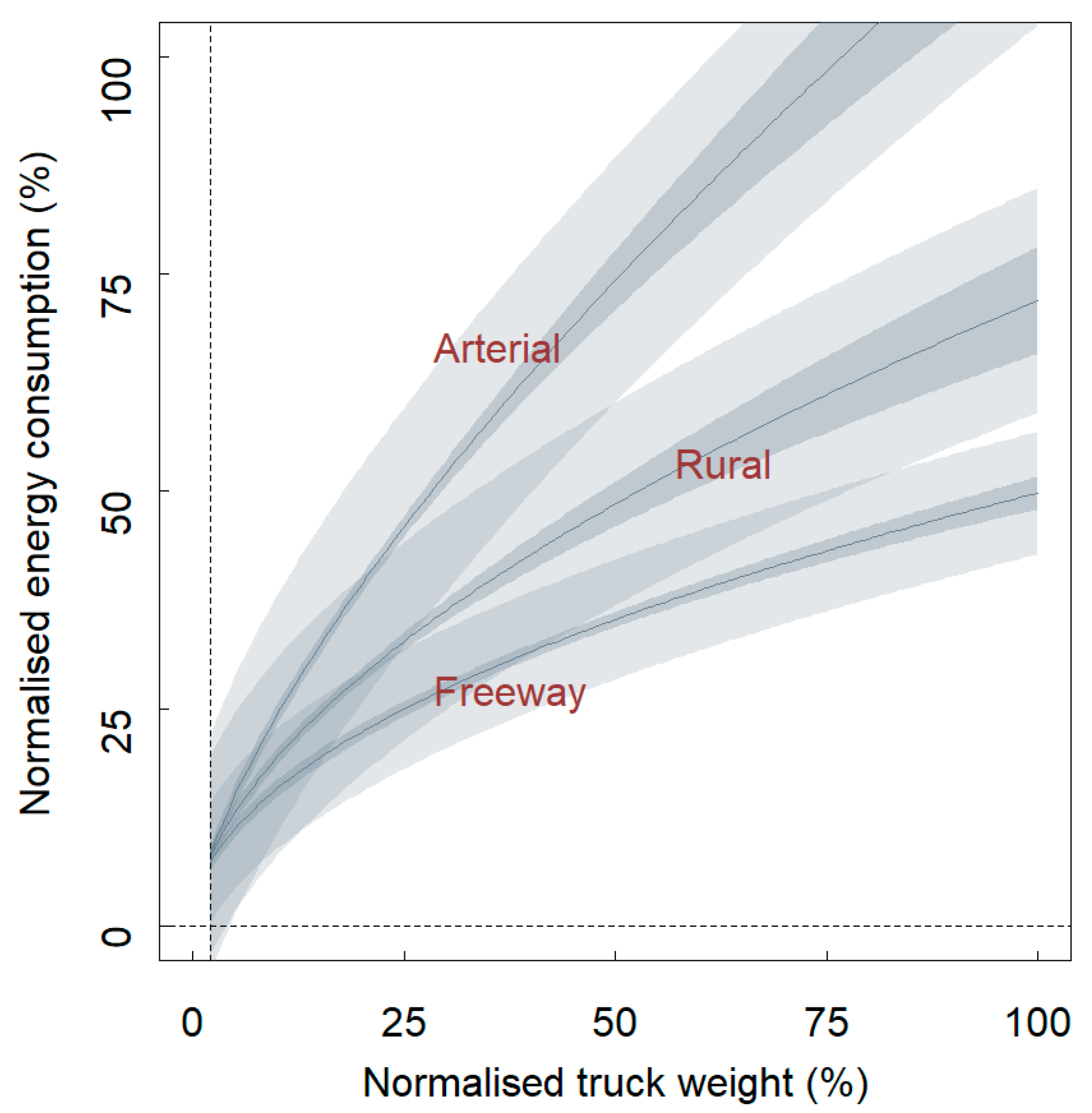
• 70% and 15% VKT share of urban driving (30 km/h);
• 5% and 10% VKT share of rural driving (75 km/h);
• 25% and 75% VKT share of highway driving (100 km/h).

Prediction performance was assessed by comparing the predictions of total fuel consumption for the Australian road transport sector with the independent fuel consumption data by fuel type for 2019. The overall difference was 0.1%, showing a good level of agreement [1]. The simulation outputs were then used to estimate representative on-road fleet-average GHG emission factors for Australian ICE trucks, fleet-average electricity consumption factors for BE trucks (including charging losses) and hydrogen consumption factors for FCE trucks (including refuelling leakage losses). The estimated uncertainty in the fleet-average operational emission factor is based on an analysis of the Survey of Motor Vehicle Use (SMVU), which is published by the Australian Bureau of Statistics (ABS). The ABS reports the average rate of fuel consumption (L/100 km) by vehicle type and the relative standard error (RSE). The standard error is a measure of the spread of estimates around the true value, and RSE is the standard error that is expressed as a percentage of the estimate. The plausible range is then defined as the 99.7% confidence interval, which is estimated as ±3 RSE.

Fuel consumption (FC) and RSE data were retrieved from the SMVU [35] for rigid trucks and articulated trucks. A diesel fuel density of 0.836 kg/L and carbon intensity of 3.16 g CO₂/g fuel was used to convert units from l/100 km to g CO₂/km. The relative uncertainty in the converted ABS figures is assumed to be ±3 RSE and follows a truncated normal distribution. The analysis shows that the plausible range for truncation is ±6% for MCVs and HCVs and ±3% for ATs, respectively. This distribution and the plausible ranges are assumed to apply to all powertrains. The results are shown in

Table 8. ICEV GHG emission factor (g CO₂-e/km) distributions for on-road driving (operational, O).

Life-Cycle Aspect	Vehicle Technology	LCA model Input Variable	Distribution	Typical Value	Plausible Min–Max Value
O 2019	MC-ICEV	eroad,ICEV,MCV	Normal, N (644, 13)	644	605–682
O 2019	HC-ICEV	eroad,ICEV,HCV	Normal, N (860, 17)	860	808–911
O 2019	AT-ICEV	eroad,ICEV,AT	Normal, N (1420, 14)	1420	1377–1462
O 2050	MC-ICEV	eroad,ICEV,MCV	Non-standard beta, B (3.57, 3.91)	547	496–603
O 2050	HC-ICEV	eroad,ICEV,HCV	Non-standard beta, B (3.52, 3.77)	731	663–804
O 2050	AT-ICEV	eroad,ICEV,AT	Triangular, T (1111, 1309, 1198)	1207	1111–1309

,

Table 9. Electricity (Wh/km) consumption distributions for on-road driving (operational, O), including battery recharging losses.

Life-Cycle Aspect	Vehicle Technology	LCA Model Input Variable	Distribution	Typical Value	Plausible Min–Max Value
O 2019	MC-BEV	εMCV	Non-standard beta, B (5.77, 11.49)	908	821–1021
O 2019	HC-BEV	εHCV	Non-standard beta, B (5.53, 11.05)	1229	1113–1384
O 2019	AT-BEV	εAT	Non-standard beta, B (3.81, 7.65)	3343	3080–3695
O 2050	MC-BEV	εMCV	Non-standard beta, B (4.14, 4.58)	646	574–720
O 2050	HC-BEV	εHCV	Non-standard beta, B (4.17, 4.68)	875	778–979
O 2050	AT-BEV	εAT	Non-standard beta, B (2.92, 3.17)	2380	2163–2622

and

Table 10. Hydrogen consumption (g H₂/km) distributions for on-road driving (operational, O), including hydrogen refuelling losses.

Life-Cycle Aspect	Vehicle Technology	LCA Model Input Variable	Distribution	Typical Value	Plausible Min–Max Value
O 2019	MC-FCEV	HMCV	Non-standard beta, B (11.42, 11.82)	45	43–48
O 2019	HC-FCEV	HHCV	Non-standard beta, B (71.83, 62.17)	61	58–64
O 2019	AT-FCEV	HAT	Gamma, G (8168.15, 45.95)	178	173–183
O 2050	MC-FCEV	HMCV	Gamma, G (564.18, 15.63)	36	33–40
O 2050	HC-FCEV	HHCV	Non-standard beta, B (3.07, 3.35)	49	45–54
O 2050	AT-FCEV	HAT	Triangular, T (130, 155, 140)	142	131–154

. It is noted that the GHG emission factor for the Australian AT fleet derived from the SMVU (1457 g CO₂/km) is 3% higher than the value predicted by n0vem (1420 g CO₂-e/km). The SMVU-derived emission factor for rigid trucks (755 g CO₂/km) lies in between the more refined classification used in n0vem for MCVs (644 g CO₂-e/km) and HCVs (860 g CO₂-e/km).

For 2050, an efficiency improvement factor was applied to the distribution definitions shown in Table 8, Table 9 and Table 10. Although some studies assume zero or small future improvements [76], significant to large gains in on-road fuel and energy efficiency are, in principle, technically possible for all vehicle technologies.

• Specifically, for compression-ignition (diesel) ICEVs, further technological “system approach” engine improvements are expected to lead to an overall 10–20% fuel efficiency improvement in 2050 (U: 0.80, 0.90). Measures to achieve this may include, but are not limited to, advanced systems for valve-train control, use of low-viscosity lubricants, variable compression ratios, re-use of waste heat and engine downsizing [49,77,78].
• BEV energy improvement is expected to be larger and is expected to occur sooner than that for FCEVs. One of these expected improvements is a significant increase in battery energy density, as was discussed in Section 3.2. It has been assumed in this study that this will largely translate into a range and power increase without affecting battery mass significantly. There are several potential improvements that will lead to significant efficiency improvements for BEVs, for instance, purpose design, in-wheel or wheel-hub electric motors rather than central engines, improved energy recuperation, decreased coasting resistance and the application of lightweight chassis components [50]. The expected improvement in energy efficiency for BEVs is assumed to be in the order of 20–30% in 2050 (U: 0.70, 0.80).
• Although some studies assume zero improvement for FCEVs [76], further improvement in the fuel-cell energy efficiency is expected from the current 50–60% to 65% in the near term and up to 70% in the long term [49,54,55]. This leads to an estimated improvement in energy efficiency for FCEVs of 15–25% in 2050 (U: 0.75, 0.85). It has been assumed in this study that this will largely translate into a range and power increase.

BEVs have larger expected efficiency improvements than FCEVs and ICEVs, which aligns with assumptions made in other studies [49,76,79,80,81]. Monte Carlo simulation and subsequent distribution fitting was used to combine the input distributions for real-world on-road fuel consumption (ICEV), electricity consumption (BEV), hydrogen consumption (FCEV), future efficiency improvement (ICEV, BEV, FCEV), battery recharging losses (BEV) and refuelling losses (FCEV) to create the input distributions presented in Table 8, Table 9 and Table 10.

Electricity and hydrogen consumption (Table 9 and Table 10) by electric vehicles still need to be converted to the functional unit (per vehicle km), which depends on the year of interest (2019 or 2050). For BEVs, electricity consumption (Table 9) is combined with the emission intensities (g CO₂-e/kWh consumed) for the grid-loss-corrected electricity generation in Australia in 2019 and 2050 (Table 5) in a Monte Carlo simulation and subsequent distribution fitting. The results are shown in

Table 11. BEV GHG emission factor (g CO₂-e/km) distributions for on-road driving (operational, O), including grid losses and battery charging losses.

Life-Cycle Aspect	Vehicle Technology	LCA Model Input Variable	Distribution	Typical Value	Plausible Min–Max Value
O 2019	MC-BEV	eroad,BEV,MCV	Non-standard beta, B (6.47, 12.41)	690	618–780
O 2019	HC-BEV	eroad,BEV,HCV	Non-standard beta, B (6.64, 13.03)	934	837–1059
O 2019	AT-BEV	eroad,BEV,AT	Non-standard beta, B (5.01, 9.58)	2541	2305–2837
O 2050	MC-BEV	eroad,BEV,MCV	Non-standard beta, B (9.71, 23.05)	53	46–64
O 2050	HC-BEV	eroad,BEV,HCV	Lognormal, L (4.27, 0.06)	72	62–86
O 2050	AT-BEV	eroad,BEV,AT	Non-standard beta, B (8.24, 19.56)	195	170–232

.

For FCEVs, hydrogen consumption (Table 10) is combined with the emission intensities (g CO₂-e/g H₂) for hydrogen production in Australia in 2019 and 2050 (Table 6) and for hydrogen losses (distribution and refuelling) in a Monte Carlo simulation and subsequent distribution fitting. The results are shown in

Table 12. FCEV GHG emission factor (g CO₂-e/km) distributions for on-road driving (operational, O), including hydrogen distribution and refuelling losses.

Life-Cycle Aspect	Vehicle Technology	LCA Model Input Variable	Distribution	Typical Value	Plausible Min–Max Value
O 2019	MC-FCEV	eroad,FCEV,MCV	Non-standard beta, B (2.51, 2.60)	529	446–623
O 2019	HC-FCEV	eroad,FCEV,HCV	Gamma, G (157.57, 0.22)	718	611–834
O 2019	AT-FCEV	eroad,FCEV,AT	Non-standard beta, B (1.57, 1.71)	2083	1795–2398
O 2050	MC-FCEV	eroad,FCEV,MCV	Location-scale t, O (2,289,788, 142, 32)	142	83–209
O 2050	HC-FCEV	eroad,FCEV,HCV	Non-standard beta, B (1.53, 1.81)	193	113–821
O 2050	AT-FCEV	eroad,FCEV,AT	Non-standard beta, B (1.67, 1.78)	560	331–814

.

Finally, changes in the truck mass (Section 3.2) will affect operational energy and fuel consumption and therefore on-road emissions. Figure 2 visualises the generalised truck-mass-correction algorithms that are used in the n0vem software for energy use in different driving conditions. These correction algorithms are used in the full LCA simulation (Section 4) to correct the operational emissions due to changes in the vehicle mass. It is noted that these corrections lead to relatively small adjustments in on-road fuel consumption and energy use (within ±12%), since this study explicitly uses fleet-average values rather than the more variable values for individual vehicles.

3.8. Truck Maintenance

The contribution of truck maintenance to the emissions performance will be added to the operational life-cycle aspect in the full simulation of all the life-cycle aspects combined (Section 4) by assuming a contribution of 4 to 7 g CO₂-e/km for all power trains and vehicle classes [2], i.e., (U: 4, 7).

3.9. Energy Infrastructure

The construction and retirement of fossil-fuel power plants, facilities involved in fossil fuel processing (such as refineries and fuel storage), hydrogen production and distribution infrastructure, as well as renewable energy sources (including solar plants, wind farms, hydropower facilities, etc.), consume energy and result in the generation of greenhouse gas (GHG) emissions.

The input distribution for fossil-fuel production was adopted from a previous study [17] where a plausible range was estimated as 2 to 30 g CO₂-e per kg of fossil-fuel produced (U: 2, 30). This distribution was combined in a Monte Carlo simulation with the distributions for real-world fuel consumption, which were derived from Table 8 after conversion from GHG emissions to real-world (diesel) fuel consumption. The sampling distributions were used to determine the best theoretical distribution through a maximum-likelihood fit. The results are shown in

Table 13. Infrastructure (I) GHG emission factor (g CO₂-e/km) distributions for Australian ICEVs.

Life-Cycle Aspect	Vehicle Technology	LCA Model Input Variable	Distribution	Typical Value	Plausible Min–Max Value
I 2019	MC-ICEV	einfra,ICEV,MCV	Uniform, U (0.4, 6.2)	3	0–6
I 2019	HC-ICEV	einfra,ICEV,HCV	Uniform, U (0.6, 8.3)	4	1–8
I 2019	AT-ICEV	einfra,ICEV,AT	Uniform, U (0.9, 13.5)	7	1–14
I 2050	MC-ICEV	einfra,ICEV,MCV	Uniform, U (0.4, 5.7)	3	0–6
I 2050	HC-ICEV	einfra,ICEV,HCV	Uniform, U (0.5, 7.6)	4	1–8
I 2050	AT-ICEV	einfra,ICEV,AT	Uniform, U (0.8, 12.3)	6	1–12

.

Input distributions for electricity generation were developed in a previous study [17] based on data from 33 LCA studies. Turconi et al. [82] reviewed 33 LCA studies, and the raw data from this study were used to determine the best theoretical distribution through a maximum-likelihood fit and the associated plausible ranges for infrastructure related GHG intensity per kWh of electricity (generated) by fuel type. The results are shown in

Table 14. GHG emission intensities (g CO₂-e/kWh generated) distributions for commissioning and decommissioning electricity generation infrastructure by fuel type.

Fuel Type	Distribution	Typical Value	Plausible Min–Max Value
Biomass	Uniform, U (0.04, 2.00)	0.45	0.04–2.00
Coal	Uniform, U (0.8, 46.0)	8.00	0.80–46.00
Gas	Triangular, T (0.60, 1.85, 3.10)	1.85	0.60–3.10
Hydro	Uniform, U (3.10, 20.00)	7.40	3.10–20.00
Oil	Triangular, T (1.00, 2.20, 3.00)	2.20	1.00–3.00
Solar	Exponential, E (0.015)	67.94	20.00–190.00
Wind	Uniform, U (3.00, 41.00)	18.93	3.00–41.00

.

The fuel type distributions defined in Table 14 were used in a Monte Carlo simulation along with the previously mentioned distributions for grid losses (T: 1.05, 1.10, 1.06) and BEV real-world energy consumption distributions (Table 9), which account for battery charging losses. The fuel-type percentages from Table 3 were used as weights in this process. The resulting sampling distributions were employed to identify the optimal theoretical distribution through a maximum-likelihood fit, and the outcomes are presented in

Table 15. Infrastructure (I) GHG emission factor (g CO₂-e/km) distributions for Australian BEVs.

Life-Cycle Aspect	Vehicle Technology	LCA Model Input Variable	Distribution	Typical Value	Plausible Min–Max Value
I 2019	MC-BEV	einfra,BEV,MCV	Non-standard beta, B (2.25, 2.82)	19	4–37
I 2019	HC-BEV	einfra,BEV,HCV	Non-standard beta, B (2.18, 2.61)	26	5–51
I 2019	AT-BEV	einfra,BEV,AT	Non-standard beta, B (2.19, 2.59)	71	15–137
I 2050	MC-BEV	einfra,BEV,MCV	Gamma, G (6.38, 0.29)	22	7–49
I 2050	HC-BEV	einfra,BEV,HCV	Lognormal, L (3.31, 0.40)	30	10–67
I 2050	AT-BEV	einfra,BEV,AT	Non-standard beta, B (2.11, 4.82)	81	28–183

.

A focus on the regional production of hydrogen seems to be required for Australia, given its vast size and long transport distances. However, no information or data could be located to inform the development of the LCA input distributions for the hydrogen production infrastructure. The infrastructure-related GHG emission factors were therefore assumed to be similar to those developed for BEVs (Table 15), and further research is recommended to develop input distributions for relevant hydrogen pathways (SMR and electrolysis with renewables).

3.10. Upstream Emissions (Fuel/Energy)

The extraction, transport, production, and distribution processes involved in obtaining refined fossil fuels like petrol and diesel consume energy and result in the generation of greenhouse gas (GHG) emissions. Data published in the international literature on well-to-wheel assessments indicate that a range of 14% to 28% of the contained energy in these fuels is consumed throughout the chain, with an estimated average value of 20% (U: 0.14, 0.28) [6,7,8,44,46,82,83]. This distribution was combined in a Monte Carlo simulation with the distributions for real-world fuel consumption derived from Table 8, after conversion from GHG emissions to real-world (diesel) fuel consumption. The sampling distributions were employed to identify the optimal theoretical distribution using the maximum-likelihood fit, and the outcomes are presented in

Table 16. Fuel/energy (F) GHG emission factor (g CO₂-e/km) distributions for Australian ICEVs.

Life-Cycle Aspect	Vehicle Technology	LCA Model Input Variable	Distribution	Typical Value	Plausible Min–Max Value
F 2019	MC-ICEV	efuel,ICEV,MCV	Location-scale t, O (2,180,536, 43, 8)	43	28–59
F 2019	HC-ICEV	efuel,ICEV,HCV	Uniform, U (37, 79)	57	37–79
F 2019	AT-ICEV	efuel,ICEV,AT	Uniform, U (63, 127)	94	63–127
F 2050	MC-ICEV	efuel,ICEV,MCV	Location-scale t, O (1,556,144, 36, 7)	36	23–51
F 2050	HC-ICEV	efuel,ICEV,HCV	Normal, N (48, 10)	49	31–68
F 2050	AT-ICEV	efuel,ICEV,AT	Non-standard beta, B (1.54, 1.79)	80	51–112

.

Upstream emissions for electricity generation are GHG emissions due to the upstream extraction, transport, production and distribution of the fossil fuels used in electricity generation. Input distributions for electricity generation were developed in a previous study [17] and are adopted here. For BEVs in 2019, real-world electricity consumption (Table 9) was combined with the upstream emission intensity value (80 g CO₂-e/kWh consumed), published as Scope 3 NGA GHG emission factors (National Greenhouse Accounts) for Australia, and a skewed t distribution to quantify the uncertainty (S: 0.94, 0.09, 1.49, 216.93), truncated at 0.75 and 1.30, in a Monte Carlo simulation and subsequent distribution fitting. For BEVs in 2050, real-world electricity consumption (Table 9) was combined with the upstream GHG emission intensities for electricity generation using a range of renewables and fossil fuels (Table 9 in [17]) and the grid-loss distribution (T: 1.05, 1,10, 1.06) in a Monte Carlo simulation and subsequent distribution fitting. The results are shown in

Table 17. Fuel/energy (F) GHG emission factor (g CO₂-e/km) distributions for Australian BEVs.

Life-Cycle Aspect	Vehicle Technology	LCA Model Input Variable	Distribution	Typical Value	Plausible Min–Max Value
F 2019	MC-BEV	efuel,BEV,MCV	Lognormal, L (4.26, 0.07)	71	58–88
F 2019	HC-BEV	efuel,BEV,HCV	Lognormal, L (4.56, 0.07)	96	78–121
F 2019	AT-BEV	efuel,BEV,AT	Lognormal, L (5.57, 0.07)	263	214–328
F 2050	MC-BEV	efuel,BEV,MCV	Weibull, W (2.67, 7.85)	7	1–16
F 2050	HC-BEV	efuel,BEV,HCV	Non-standard beta, B (4.39, 11.13)	10	1–22
F 2050	AT-BEV	efuel,BEV,AT	Non-standard beta, B (4.38, 11.32)	26	4–61

. It has conservatively been assumed that the proportion of battery electric truck operators that generate their own sustainable electricity (solar panels) for battery recharging is zero.

For FCEVs, upstream emissions relate to the extraction, transport, production and distribution of natural gas for the SMR process and water for both SMR and electrolysis. For natural gas, the same assumption as was previously made for fossil fuels was used, namely that up to 14 to 28% of the contained energy in the fuels is consumed within the chain, with an estimated average value of 20% (U: 0.14, 0.28). Assuming that about 3.0 to 3.5 times the amount of natural gas is required to produce 1 kg of hydrogen, reflecting the LHV ratio and an assumed 70 to 80% SMR conversion efficiency (U: 3.0, 3.5), the two uniform distributions were combined in a Monte Carlo simulation with the distributions for on-road hydrogen consumption (Table 9). As mentioned before, it was assumed that about 75% and 10% of hydrogen is produced and distributed with fossil fuels (SMR) in 2019 and 2050, respectively. The carbon intensity of natural gas is assumed to be 2.74 g CO₂-e/g fuel.

The sampling distributions were employed to identify the optimal theoretical distribution using a maximum-likelihood fit, and the outcomes are presented in

Table 18. Upstream (U) GHG emission factor (g CO₂-e/km) distributions for Australian FCEVs.

Life-Cycle Aspect	Vehicle Technology	LCA Model Input Variable	Distribution	Typical Value	Plausible Min–Max Value
U 2019	MC-FCEV	eupstream,FCEV,MCV	Normal, N (64, 13)	64	40–91
U 2019	HC-FCEV	eupstream,FCEV,HCV	Location-scale t, O (2,191,700, 86, 17)	86	54–122
U 2019	AT-FCEV	eupstream,FCEV,AT	Non-standard beta, B (2.01, 2.16)	249	157–355
U 2050	MC-FCEV	eupstream,FCEV,MCV	Triangular, T (3.8, 10.3, 5.8)	7	4–10
U 2050	HC-FCEV	eupstream,FCEV,HCV	Triangular, T (5.4, 13.9, 7.9)	9	6–14
U 2050	AT-FCEV	eupstream,FCEV,AT	Non-standard beta, B (1.91, 2.59)	27	16–40

.

Upstream emissions related to clean-water production and delivery for electrolysis was set to zero in the absence of accurate input information. But it is noted that these emissions could be significant and would be a function of the production method (e.g., desalination plants) and delivery method (pipelines, trucks). The total upstream emissions for hydrogen are therefore likely to be underestimated, and further research is recommended.

3.11. Vehicle Disposal and Recycling

Evaluating the impacts of recycling and disposal in a life-cycle assessment can pose significant challenges for a product as intricate as a truck. GHG emissions from the end-of-life phase of a vehicle have been observed to be relatively minor compared with the operational use phase, and, as a result, they are frequently either overlooked or incorporated into the vehicle manufacturing life-cycle aspect [8,84,85]. Generally, a vehicle’s end-of-life impact (recycling and disposal) has a limited contribution in terms of environmental impacts [47,70]. In the previous related study for passenger vehicles [17], GHG emission rates due to disposal were estimated to be only 0.14% and 0.20% of the life-cycle emissions for ICEVs and BEVs, respectively. Despite the uncertainty, it is clear that emission impacts regarding end-of-life recycling or disposal processes are trivial.

The input distributions for vehicle recycling and disposal were derived from the previous study [17] after consideration of the differences in the PV and truck vehicle mass (Table 2) and lifetime mileage (Section 3.1), and the results are shown in

Table 19. Disposal (D) GHG emission factor (g CO₂-e/km) distributions for Australian trucks.

Life-Cycle Aspect	Vehicle Technology	LCA Model Input Variable	Distribution	Typical Value	Plausible Min–Max Value
D	MC-ICEV	edisposal,ICEV,MCV	Uniform, U (0.1, 1.4)	1	0–1
D	HC-ICEV	edisposal,ICEV,HCV	Uniform, U (0.2, 4.1)	2	0–4
D	AT-ICEV	edisposal,ICEV,AT	Uniform, U (0.1, 2.7)	1	0–3
D	MC-EV	edisposal,EV,MCV	Uniform, U (0.1, 1.7)	1	0–2
D	HC-EV	edisposal,EV,HCV	Uniform, U (0.3, 5.6)	3	0–6
D	AT-EV	edisposal,EV,AT	Uniform, U (0.2, 3.3)	2	0–3

for 2019. It is noted that disposal emission factors are assumed to be the same for BEVs and FCEVs; these are noted as EVs (electric vehicles).

It is noted that the impact of disposal is dependent on the extent of recycling of the vehicle materials, which is already high with end-of-life EU targets stipulating that 85% of the vehicle mass should be re-used, recovered and recycled [37]. The recycling process at the end of a vehicle’s life, including the recycling of batteries, will partially offset emissions generated during the manufacturing process [14]. Another consideration is second-life use of spent BEV batteries, which was discussed before and which can further decrease the vehicle’s battery carbon footprint by 50% [7].

The recovery and recycling of materials utilized in BEV batteries have experienced a notable increase, driven by the elevated costs associated with the raw materials used in their production [70], which reduces the impact of vehicle manufacturing when recycled materials are used. Recycling of fuel-cell systems require new methods, but this is considered feasible [37]. It seems reasonable to assume that future truck disposal practices will include significant recycling processes and reflect the general decarbonisation of energy systems, so the reduction factor in 2050 is expected to vary between 10% and 50% of the 2019 values (U: 0.10, 0.50).

4. Results and Discussion

The development and examination of individual parametric input distributions was discussed in the previous section. In the full probabilistic LCA, all the life-cycle aspects are combined. Common inputs for different life-cycle aspects (e.g., mass of batteries, fuel-cell systems, tare vehicle mass, battery capacity) are passed on during the full simulation (n = 1 million) for the different life-cycle aspects to ensure valid and internally consistent outcomes. The results of the full simulation are discussed in this section, providing a probabilistic life-cycle technology assessment for the 18 combinations of truck vehicle class, powertrain technology and year.

4.1. Average Life-Cycle GHG Emission Factors for Trucks

The simulation results are visualised as PDFs in Figure 3 for 2019 and 2050.

Table 20. Life-cycle GHG emission factor (g CO₂-e/km) statistics.

Vehicle Class	Powertrain Technology	Year of Assessment	Mean	Median	Lower 99.7% Confidence Limit (mean)	Upper 99.7% Confidence Limit (mean)
MCV	ICEV	2019	714	714	658	773
MCV	BEV	2019	909	907	792	1059
MCV	FCEV	2019	799	790	603	1139
HCV	ICEV	2019	981	981	899	1067
HCV	BEV	2019	1171	1167	1011	1380
HCV	FCEV	2019	1041	1030	784	1483
AT	ICEV	2019	1563	1563	1491	1636
AT	BEV	2019	3070	3062	2750	3471
AT	FCEV	2019	2627	2623	2166	3239
MCV	ICEV	2050	598	597	531	670
MCV	BEV	2050	104	102	79	140
MCV	FCEV	2050	198	198	123	288
HCV	ICEV	2050	806	805	711	908
HCV	BEV	2050	141	140	104	192
HCV	FCEV	2050	258	258	160	375
AT	ICEV	2050	1310	1310	1195	1430
AT	BEV	2050	337	331	257	458
AT	FCEV	2050	697	697	432	1001

also presents summary statistics for these distributions, i.e., the average life-cycle emission factors and the plausible range of these mean values (99.7% CI), which reflects the variability and uncertainty in the mean values. A PDF is a curve that quantifies the probability that the variable of interest falls within a particular range of values. The PDF is non-negative, and the area under the curve equals one. The position and shape of the distributions provide information regarding the typical values (e.g., mean, median) and the variability and uncertainty in these values. A wide distribution suggests a higher level of uncertainty, whereas a narrow distribution suggests a relatively robust emissions performance.

It is important to note again that the 2050 scenario is not necessarily restricted to 2050. It would apply to any current situation where renewable low-carbon energy is used for the different life-cycle aspects. Examples are the use of solar panels to charge batteries or the use of grid electricity that is currently generated in Tasmania with almost 95% renewables [17].

The full life-cycle simulation (Figure 3 and Table 20) shows that the absolute and relative life-cycle GHG emissions performance depends on the vehicle class, powertrain and year of assessment. For the recent past scenario (2019), ICE trucks perform best overall, with average life-cycle GHG emission factors that are 27% (MCV), 19% (HCV) and 96% (AT) higher for battery electric powertrains due to e.g. the high emission intensity of electricity generation in 2019, and 12% (MCV), 6% (HCV) and 68% (AT) higher for fuel-cell electric powertrains.

For the future situation (2050), the picture changes, where BEV and FCEV technology in combination with the emission intensities of a decarbonised Australian electricity grid and a mostly green hydrogen-production pathway provide large reductions. Battery electric powertrains provide large reductions in the average ICEV life-cycle GHG emission factors of 83% (MCV), 83% (HCV) and 74% (AT). Fuel-cell electric powertrains also provide substantial reductions, but these are not as large as those for battery electric trucks. FCEV reduces the life-cycle GHG emission factors for ICEV by 67% (MCV), 68% (HCV) and 47% (AT), respectively. Although conventional diesel truck technology exhibits improvements in operational energy efficiency, they cannot match the strong improvements in the GHG emissions performance of EVs, and of BEVs in particular.

Figure 4 shows the progression in the confidence intervals over time. Generation of this information is one of the benefits of pLCA: it provides another layer of information where the uncertainty and the robustness of the absolute results can be assessed.

Figure 4 shows that the uncertainty and spread in the mean life-cycle emission factors for ICEV is relatively small, which is shown by the relatively narrow band for all vehicle classes. It also shows that the ICEV truck performance improves with about 5–20% in the period 2019 to 2050. In contrast, the uncertainty and spread in the mean life-cycle emission factors for FCEV is relatively large, which is shown by the relatively wide band for this technology.

In addition, the uncertainty and spread (absolute values, not relative) converges and is reduced in 2050 compared with 2019. The uncertainty and spread in the mean life-cycle emission factors for BEV is also relatively small. Similarly to FCEV, the uncertainty and spread (absolute values, not relative) converges and is reduced in 2050 compared with 2019.

Although the average life-cycle GHG emission factor for diesel trucks (ICEVs) generally outperforms electric vehicles (BEVs and FCEVs) in 2019, it is the other way around in 2050. It is important to note that BEVs are expected to perform particularly well in the 2050 simulation. They show the greatest reductions in the overall emissions performance, including a further 45–52% reduction in GHG emissions per kilometre compared with FCEVs.

In addition, the spread (variability + uncertainty) in the average GHG emissions performance for BEVs in 2050 is the smallest, varying between 60–201 g CO₂-e/km. In comparison, the range is 139–235 g CO₂-e/km for ICEVs and 65–569 g CO₂-e/km for FCEVs. The uncertainty is high for hydrogen trucks due to the propagation of relatively large uncertainty and variability in the inputs.

This suggests that, out of the three powertrain options, battery electric trucks will deliver the greatest and most robust emission reductions for all vehicle classes, and therefore carry the lowest risk of not delivering the anticipated life-cycle emissions performance. Fuel-cell electric hydrogen trucks, on the other hand, will also reduce emissions compared with ICE trucks, but these reductions are not as great, and, relevantly, they are the least robust of all the technology options. They therefore carry the highest risk of potentially not achieving the expected reductions.

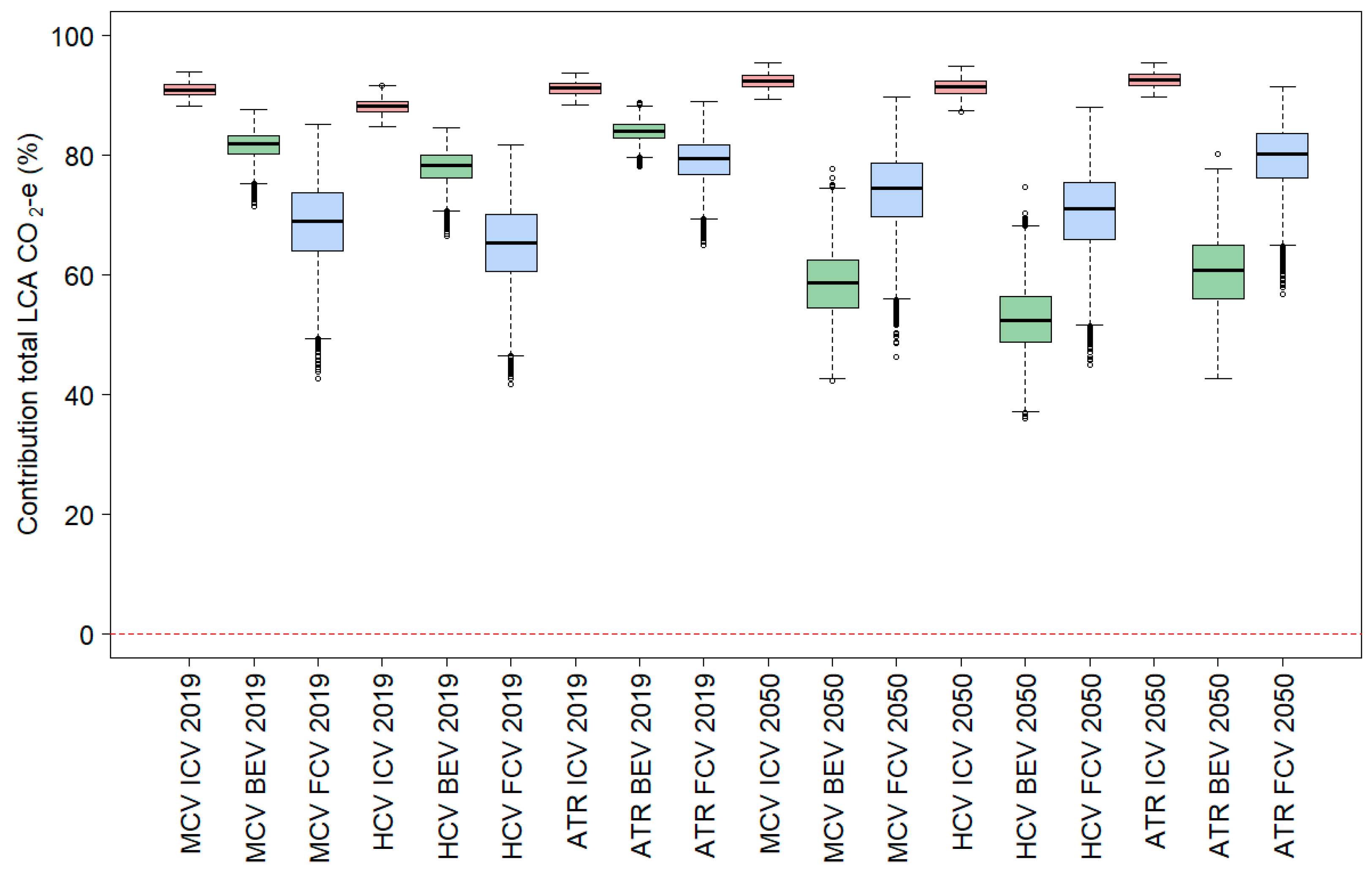
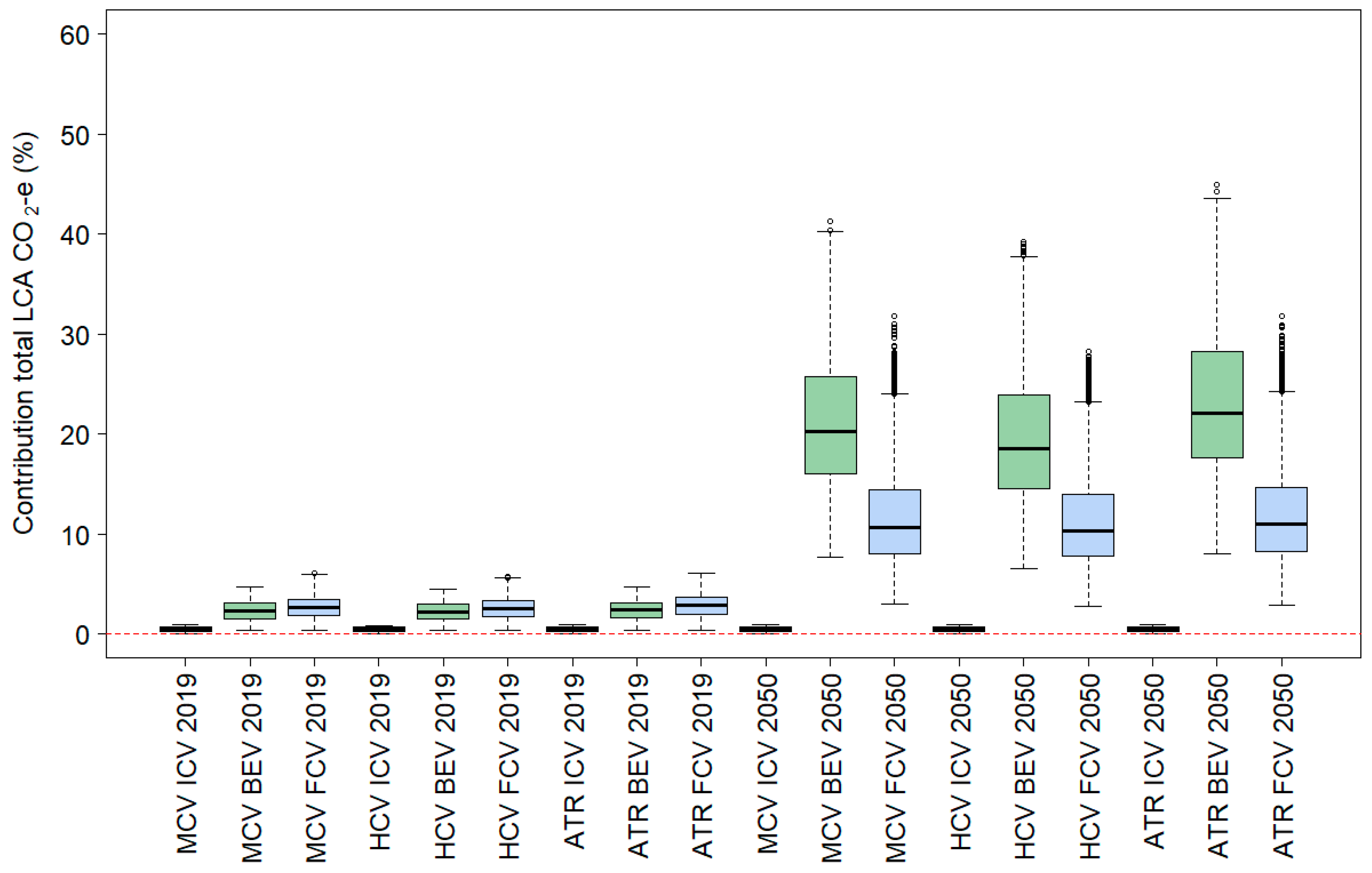
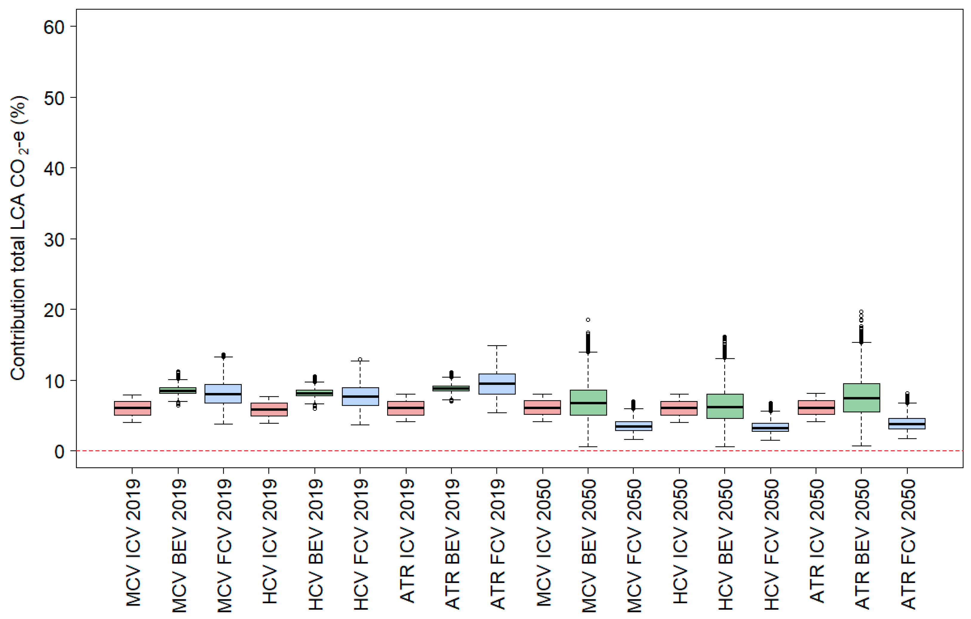
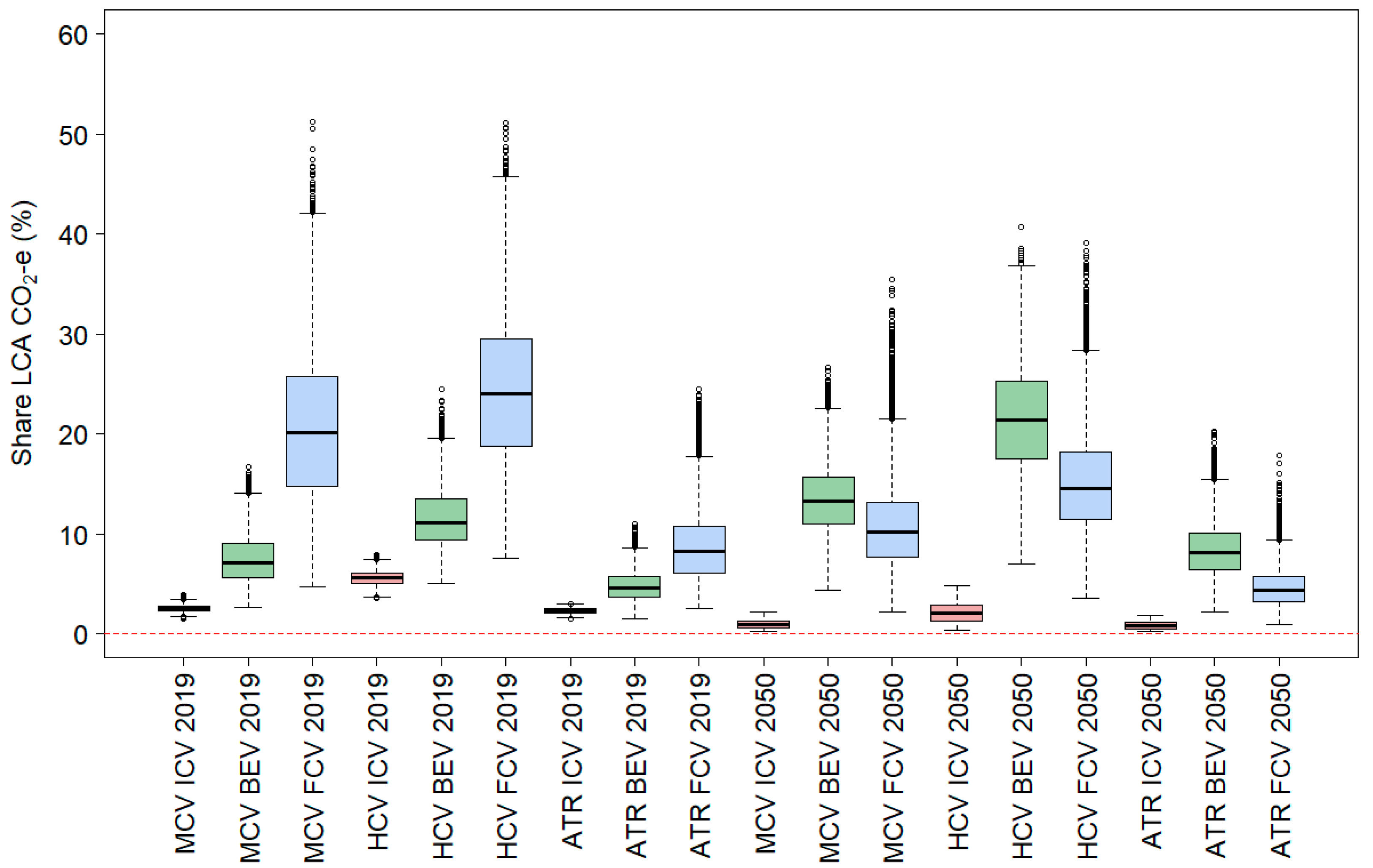
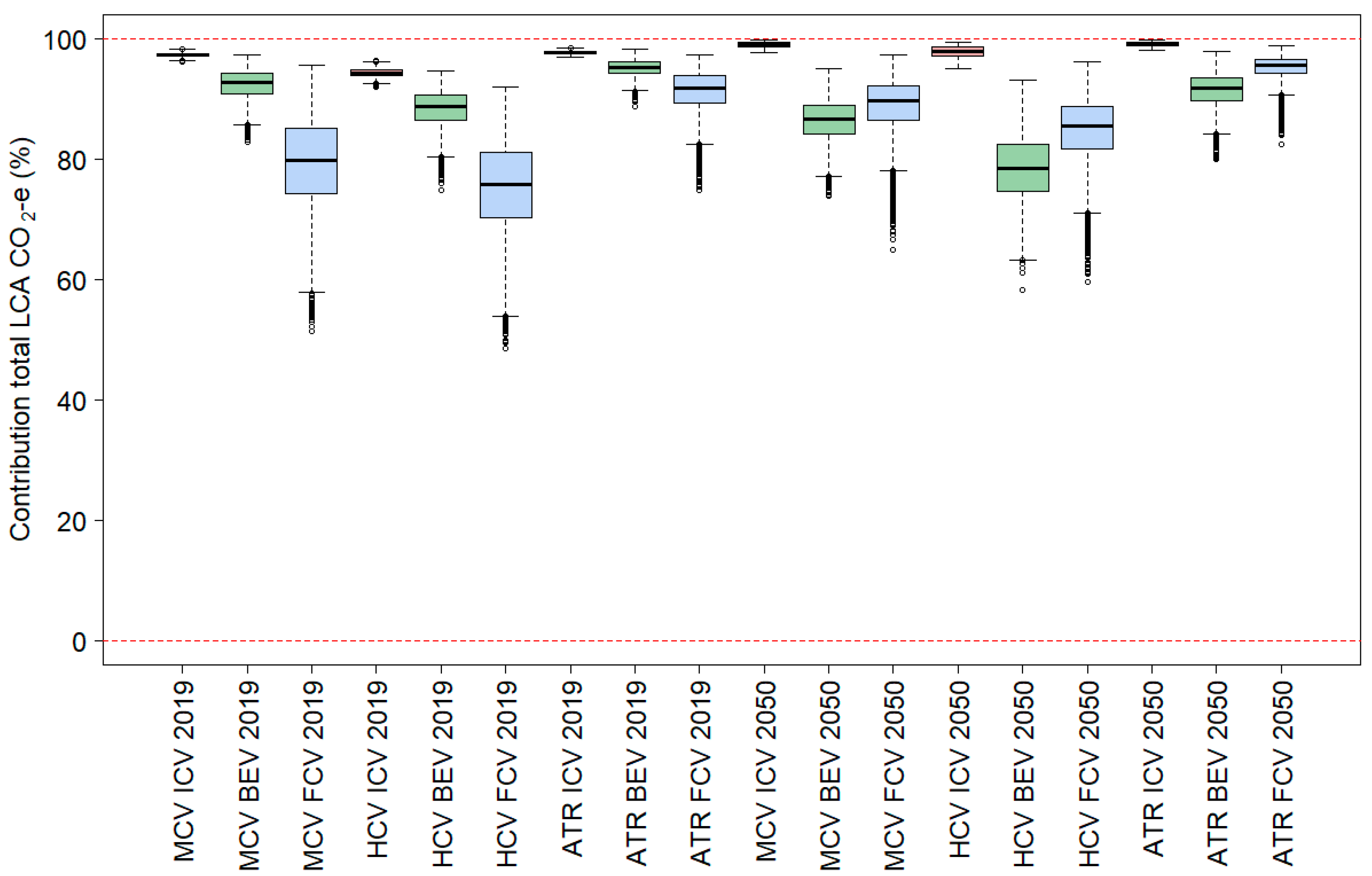
4.2. The Relevance of Different Life-Cycle Aspects

The simulation results can be examined to assess the relative importance of the different life-cycle aspects for the total GHG emission rates. Each one of the million simulations for each of the 18 combinations of vehicle class, powertrain category and year of assessment will result in different shares of the five life-cycle aspects. The results are therefore presented in terms of summary statistics and visualised with box plots.

Table 21. Mean and plausible range (99.7% CI, within brackets) of the percentage share of the life-cycle GHG emission factor (g CO₂-e/km) for each life-cycle aspect by vehicle class, powertrain technology and year.

Vehicle Class	Powertrain Technology	Year of Assessment	Vehicle Manufacturing	Upstream Infrastructure	Upstream Fuel and Energy	Operational (on-Road + Maintenance)	Disposal and Recycling
MCV	ICEV	2019	2.5 (1.7–3.4)	0.5 (0.1–0.9)	6.0 (4.1–7.9)	91.0 (88.6–93.5)	0.1 (0.0–0.2)
MCV	BEV	2019	7.4 (3.1–15.6)	2.3 (0.5–4.4)	8.5 (6.9–10.4)	81.6 (74.0–86.8)	0.1 (0.0–0.2)
MCV	FCEV	2019	20.5 (6.1–44.3)	2.7 (0.5–5.6)	8.1 (4.3–13.0)	68.6 (47.7–83.3)	0.1 (0.0–0.3)
HCV	ICEV	2019	5.3 (3.6–7.3)	0.4 (0.1–0.8)	5.8 (3.9–7.7)	88.2 (85.2–91.2)	0.2 (0.0–0.4)
HCV	BEV	2019	11.4 (5.7–21.2)	2.2 (0.4–4.2)	8.2 (6.5–10.1)	78.0 (69.1–84.0)	0.3 (0.0–0.5)
HCV	FCEV	2019	24.3 (9.4–47.1)	2.5 (0.5–5.3)	7.8 (4.1–12.4)	65.2 (45.1–80.0)	0.3 (0.0–0.7)
AT	ICEV	2019	2.2 (1.6–2.8)	0.5 (0.1–0.9)	6.0 (4.1–7.9)	91.2 (88.9–93.7)	0.1 (0.0–0.2)
AT	BEV	2019	4.7 (1.8–9.5)	2.4 (0.5–4.5)	8.8 (7.3–10.7)	84.0 (79.1–88.0)	0.1 (0.0–0.1)
AT	FCEV	2019	8.6 (2.8–21.9)	2.8 (0.6–5.7)	9.5 (5.6–14.2)	79.1 (66.4–87.7)	0.1 (0.0–0.1)
MCV	ICEV	2050	0.9 (0.2–2.0)	0.5 (0.1–0.9)	6.1 (4.1–8.0)	92.5 (89.9–95.2)	0.0 (0.0–0.1)
MCV	BEV	2050	13.1 (5.1–23.7)	21.3 (8.4–39.3)	6.9 (1.1–15.6)	58.4 (43.6–73.3)	0.3 (0.0–0.9)
MCV	FCEV	2050	10.8 (3.0–30.1)	11.6 (3.6–27.6)	3.5 (1.7–6.6)	74.0 (52.5–87.6)	0.1 (0.0–0.5)
HCV	ICEV	2050	2.0 (0.4–4.4)	0.5 (0.1–0.9)	6.0 (4.1–8.0)	91.4 (87.9–94.8)	0.1 (0.0–0.2)
HCV	BEV	2050	20.8 (8.1–35.4)	19.6 (7.5–37.6)	6.4 (1.0–14.5)	52.6 (38.5–68.7)	0.6 (0.0–2.1)
HCV	FCEV	2050	14.8 (4.3–34.9)	11.1 (3.5–26.5)	3.4 (1.7–6.3)	70.4 (48.9–85.7)	0.4 (0.0–1.3)
AT	ICEV	2050	0.8 (0.2–1.7)	0.5 (0.1–0.9)	6.1 (4.2–8.0)	92.6 (90.0–95.2)	0.0 (0.0–0.1)
AT	BEV	2050	8.3 (2.4–17.7)	23.5 (9.5–42.4)	7.7 (1.2–17.1)	60.4 (44.4–76.1)	0.2 (0.0–0.5)
AT	FCEV	2050	4.6 (1.2–13.1)	11.9 (3.7–28.5)	3.9 (1.9–7.4)	79.6 (61–90.5)	0.1 (0.0–0.3)

presents the summary statistics for these distributions, i.e., the lower and upper confidence limits of the average percentage contribution to the life-cycle GHG emission rates for each life-cycle aspect. Figure 5 and Figure 6 show the life-cycle emission results for the so-called “vehicle cycle” (manufacturing + disposal) and “fuel cycle” (infrastructure + fuel/energy+ operational) in box plots. Appendix B includes similar plots for the individual life-cycle aspects.

It is clear from Table 21 and Figure 5 and Figure 6 that operational emissions (on-road driving and vehicle maintenance) dominate the life-cycle emissions for all vehicle classes, powertrain categories and years, with average contributions varying from 53% (HCV, BEV, 2050) to 93% (AT, ICEV, 2050). In contrast, disposal and recycling make negligible to small contributions, varying on average from 0.03% (AT ICEV 2050) to 0.63% (HCV BEV 2050).

Vehicle manufacturing makes a relatively small contribution to life-cycle emissions from ICEVs, on average between approximately 1% to 5%. For BEVs and FCEVs, this is significantly higher, typically in the order of 5% to 20% and 5% to 25%, respectively.

The contribution of infrastructure-related emissions to life-cycle emissions was typically small for ICEVs (less than 1%) and were slightly higher for BEVs and FCEVs in 2019 (typically 2–3%). The contribution of infrastructure-related emissions for BEV and FCEV increases significantly in 2050 (10–25%), but this shift is mainly caused by a large drop in the life-cycle emission rates for these technologies. Finally, upstream emissions due to the production of fuels and energy typically make up 6% of the life-cycle emissions for ICE trucks. For battery electric trucks, this is slightly higher, with typical contributions of 6–9%, and this is more variable for fuel-cell electric hydrogen trucks, with typical contributions of 3–10%.

Finally, Figure 7 and Figure 8 repeat the life-cycle emission factor distributions presented in Figure 2 (Section 4.1), but this time, the distributions are also split into the main life-cycle aspects assessed in this study, i.e., the “vehicle cycle” aspects (vehicle manufacturing and vehicle disposal/recycling) and three “fuel cycle” aspects, namely fuel/energy infrastructure, fuel/energy upstream and operational (on-road and maintenance) emissions.

These charts visualise and summarise important findings from this study:

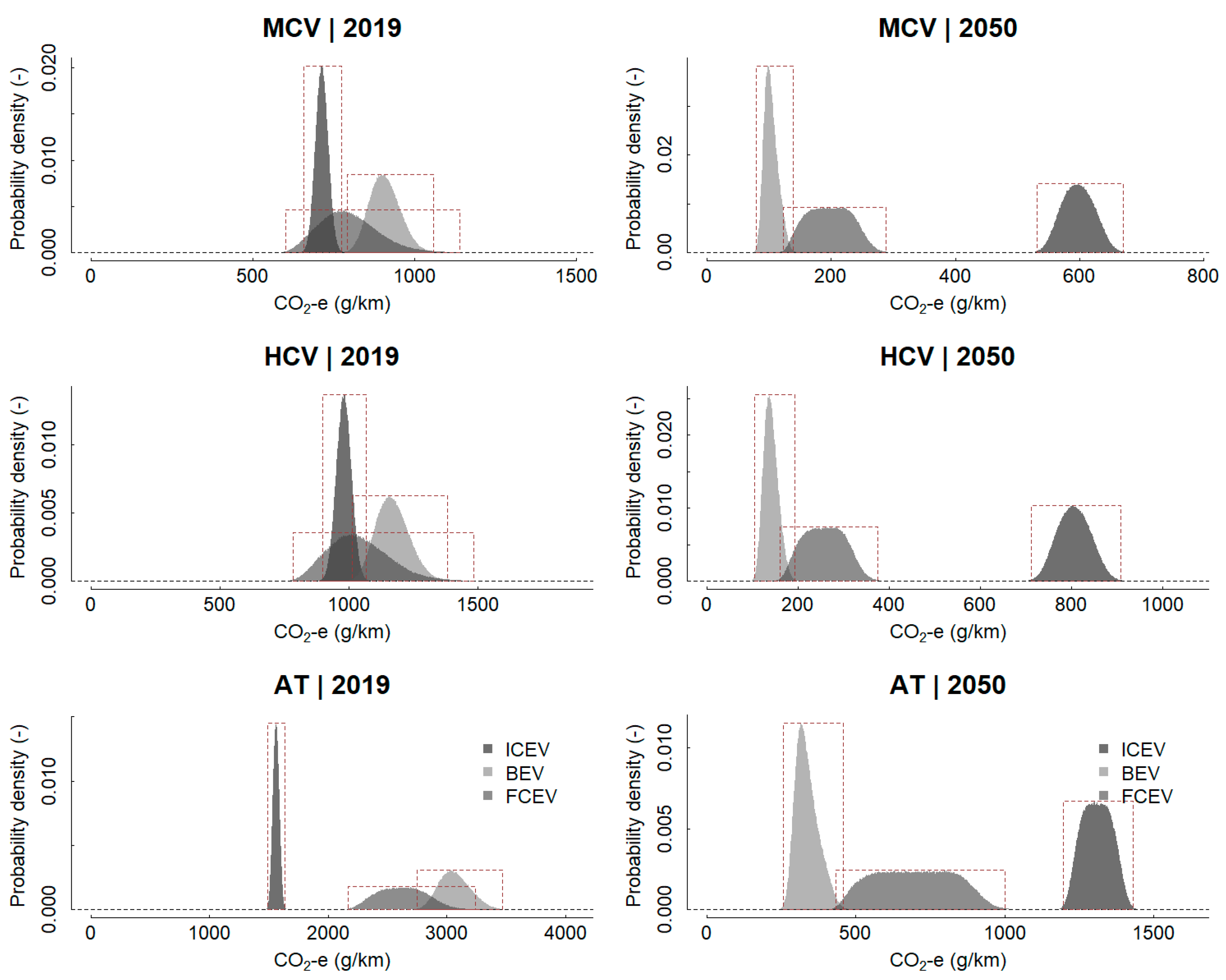
• First, it is clear that life-cycle emission factor distributions for trucks vary widely in magnitude, range and shape. They all depend on the year of assessment, truck vehicle class and powertrain technology.
• Second, any cost-effective emission reduction policies would naturally favour truck types that have narrow life-cycle GHG emissions distributions, which are as close to zero emissions as possible. They represent the maximum potential for emissions reduction and are the most robust and least uncertain technology choice. Whereas diesel trucks appear to have had the best life-cycle emissions performance in 2019, the situation is the inverse in 2050 (or in a more decarbonised situation). The simulation suggests that battery electric trucks are expected to achieve the greatest and most reliable and robust reductions in life-cycle GHG emissions.
• Third, the contribution of different life-cycle aspects is quite different, and this is particularly clear when diesel trucks are compared with electric trucks.

4.3. Comparison to Other Studies

The sixth IPCC Assessment Report [20] delivers a comprehensive review of GHG life-cycle transport emission intensities for road freight. IPCC [20] presents the results for medium-duty trucks (MDT) and heavy-duty trucks (HDT), with a 50% payload each. To compare these with the results from this study, the life-cycle GHG emission estimates were normalised for payload (Table 2). It is noted, however, that the results can only be compared in a general manner. For instance, the IPCC data for ICEVs were not organised as present (~2019) and future (~2050), but rather reflect differences in vehicle characteristics and operating efficiencies reported in the scientific literature.

In a general sense, the range of life-cycle emissions for freight trucks normalised for payload align well with the plausible range determined in this study. In both studies, the emission intensities for electric trucks (BEVs and FCEVs) similarly tend to have the lowest values when based on a renewable energy supply.

Two main differences become clear after an examination of Figure 9, when this study is compared with the IPCC [20]:

• First, this study estimates low emission intensities (per tonne km) for heavy articulated trucks (AT), but it is unclear if these heavy vehicles were included in the IPCC data. Medium-duty trucks (MDT, Figure 9) in IPCC [20] refer to the US American classification for trucks with gross vehicle masses between 7 tonnes and 13 tonnes, while heavy-duty trucks (HDT) refer to trucks with vehicle masses > 16.5 tonnes [86]. In this study, articulated trucks are defined as trucks > 25 tonnes, and the AT modelled in this study has a gross vehicle mass of 90 tonnes (Table 2).
• Second, this study estimates a significantly wider plausible range in the life-cycle emissions performance of hydrogen trucks (FCEV), whereas the IPCC estimates quite a narrow range. This is an interesting result. Our study suggests that the elevated uncertainty in several life-cycle aspects for FCEVs can produce the highest emission intensities for all technology classes.

5. Conclusions

This probabilistic LCA research study for trucks finds that the relative and absolute life-cycle GHG emissions performance strongly depends on the vehicle class, powertrain and year of assessment (reflecting the energy mix). In fact, the life-cycle emission factor distributions for trucks vary widely in magnitude, range and shape. They all depend on the year of assessment, truck vehicle class and powertrain technology.

The study has generally been conservative in the assessment of electric-vehicle technology options (e.g., not including the use of solar panels to charge batteries by truck operators). Importantly, LCA impacts have been assessed for two stationary situations, i.e., 2019 and a future decarbonised situation (10% fossil fuels). Important processes that affect life-cycle emissions, such as decarbonisation of the electricity grid, are, however, time-dynamic processes. The lifetime of trucks spans several decades, which means that a time-dependent (e.g., year-by-year) simulation of certain LCA aspects (operational and upstream emissions in particular) would provide a more accurate assessment of the life-cycle emissions performance and would likely be of significant benefit to the LCA performance of electric vehicles (refer to Section 6).

For the recent past situation, the modelling suggests that diesel trucks have the lowest life-cycle GHG emissions due to the high carbon-emission intensity of the Australian electricity grid (mainly coal) and of hydrogen production (mainly steam–methane reforming). The picture is, however, very different for a more decarbonised situation, where battery electric trucks, in particular, provide large reductions (about 75–85%) in the life-cycle GHG emissions. Fuel-cell electric (hydrogen) trucks also provide substantial reductions (about 50–70%), though not as large as those for battery electric trucks. Battery electric trucks are expected to perform particularly well in the decarbonised simulation, showing the greatest reductions in life-cycle emissions, including a further 45–50% reduction in GHG emissions per kilometre compared with hydrogen (fuel-cell) trucks.

The pLCA also provides useful information on the robustness and uncertainty in these results. The life-cycle GHG emission performance of hydrogen trucks has the largest uncertainty of all the powertrains considered, which reflects the uncertainty and general lack of information for this technology. They therefore carry a high risk of potentially not achieving the expected emission reductions. Battery electric trucks show the smallest uncertainty in the average GHG life-cycle emissions in the decarbonised situation, with a spread in emission factors varying between 60–201 g CO₂-e/km. In comparison, the spread or range is 139–235 g CO₂-e/km for diesel trucks and 65–569 g CO₂-e/km for hydrogen trucks, as predicted for 2050. This suggests that, out of the three powertrain options, battery electric trucks are expected to deliver the largest and most robust emission reductions for all vehicle classes, as long as the electricity mix is largely generated from renewables. They carry the lowest risk of not delivering the anticipated reductions in life-cycle GHG emissions.

In terms of the contributions of different life-cycle aspects to the GHG emissions performance, operational emissions (on-road driving and vehicle maintenance) dominate the life-cycle emissions for all vehicle classes, powertrain categories and years. However, their relative contribution varies substantially from about 50–60% for battery electric trucks to over 90% for diesel trucks in the (future) decarbonised situation. Disposal and recycling make a negligible contribution to all technology classes (<1%). Vehicle manufacturing makes a relatively small contribution to life-cycle emissions for diesel trucks (<5%) but is an important aspect for electric trucks (5% to 25%). Upstream emissions (fuel and infrastructure) make up the remainder, contributing about 5% to total life-cycle emissions for diesel trucks and 10–30% for electric trucks. Note that high contribution rates are mainly caused by a large drop in the total life-cycle emission rates for electric trucks.

6. Recommendations for Future Work and Refinement

Update the modelling at regular intervals—This LCA research study made use of the best available information to assess the “fleet-average” life-cycle performance of three typical truck sizes and three powertrains. It will be important to update these results once new information comes to light.

Expand the scope of assessment—Some aspects were not yet included due to a lack of information (e.g., impacts of re-engining diesel trucks) or the restricted scope of the study, and it is recommended to include these in the future. Some technologies such as catenary trucks, direct hydrogen combustion trucks, hybrid trucks and e-fuel trucks have not been included in this study and may be of interest in future work. Further refinement of the truck classification would lead to a more detailed assessment of life-cycle emissions. Consideration of other life-cycle assessment variables in the probabilistic assessment, such as cost, the combination of costs and emissions (cost-effectiveness), impacts of road infrastructure building and maintenance, and specific aspects, such as the specific constraints on technology availability, would provide useful information. It would also be useful to apply the pLCA method to specific makes/models of trucks (rather than the fleet-average performance, which was the focus of this paper) to explore the life-cycle performance and its variability and uncertainty in specific case studies.

Increase the time resolution of the simulation—It would be useful to repeat the assessment for intermediate years (e.g., 2030, 2040) to determine the non-linear trajectory of life-cycle emissions for the different vehicle classes and powertrains. In addition, a simulation of life-cycle emissions year-by-year would give a more accurate assessment and would likely be of significant benefit to the life-cycle emissions performance of electric vehicles due to the rapidly improving emission intensity of electricity generation and hydrogen production, as well as improved system durability.

References

1. Smit, R. An independent and detailed assessment of greenhouse gas emissions, fuel use, electricity and energy consumption from Australian road transport in 2019 and 2050. Air Qual. Clim. Chang. 2023, 57, 30–41. Available online: https://www.transport-e-research.com/publications (accessed on 27 November 2023).
2. O’Connell, A.; Pavlenko, N.; Bieker, G.; Searle, S. A Comparison of the Life-Cycle Greenhouse Gas Emissions of European Heavy-Duty Vehicles and Fuels, February 2023; 1500 K Street NW, Suite 650; International Council on Clean Transportation (ICCT): Washington, DC, USA, 2005. [Google Scholar]
3. European Parliament. CO2 Emissions from Cars: Facts and Figures (Infographics). European Parliament, News. 2023. Available online: https://www.europarl.europa.eu/news/en/headlines/society/20190313STO31218/co2-emissions-from-cars-facts-and-figures-infographics (accessed on 10 October 2023).
4. Cullen, D.A.; Neyerlin, K.C.; Ahluwalia, R.K.; Mukundan, R.; More, K.L.; Borup, R.L.; Weber, A.Z.; Myers, D.J.; Kusoglu, A. New roads and challenges for fuel cells in heavy-duty transportation. Nat. Energy 2021, 6, 462–474. [Google Scholar] [CrossRef]
5. Australian Government. Australia’s National Greenhouse Accounts; Australian Government (AG): Canberra, Australia, 2023. Available online: https://ageis.climatechange.gov.au/ (accessed on 27 November 2023).
6. Nordelöf, A.; Messagie, M.; Tillman, A.M.; Söderman, M.L.; Van Mierlo, J. Environmental impacts of hybrid, plug-in hybrid, and battery electric vehicles—What can we learn from life-cycle assessment? Int. J. Life Cycle Assess. 2014, 19, 1866–1890. [Google Scholar] [CrossRef]
7. Helmers, E.; Dietz, J.; Weiss, M. Sensitivity analysis in the life-cycle assessment of electric vs. combustion engine cars under approximate real-world conditions. Sustainability 2020, 12, 1241. [Google Scholar] [CrossRef]
8. Samaras, C.; Meisterling, K. Life-cycle assessment of greenhouse gas emissions from plug-in hybrid vehicles: Implications for policy. Environ. Sci. Technol. 2008, 42, 3170–3176. [Google Scholar] [CrossRef]
9. ISO 14040:2006; Environmental Management—Life-Cycle Assessment—Principles and Framework. International Organization for Standardization: Geneva, Switzerland, 2006.
10. ISO 14044:2006; Environmental Management—Life-Cycle Assessment—Requirements and Guidelines. International Organization for Standardization: Geneva, Switzerland, 2006.
11. ISO 14067:2018; Greenhouse Gases—Carbon Footprint of Products—Requirements and Guidelines for Quantification. International Organization for Standardization: Geneva, Switzerland, 2006.
12. Noshadravan, A.; Cheah, L.; Roth, R.; Freire, F.; Dias, L.; Gregory, J. Stochastic comparative assessment of life-cycle greenhouse gas emissions from conventional and electric vehicles. Int. J. Life Cycle Assess. 2015, 20, 854–864. [Google Scholar] [CrossRef]
13. Wang, Z.; Karki, R. Exploiting PHEV to augment power system reliability. IEEE Trans. Smart Grid 2016, 8, 2100–2108. [Google Scholar] [CrossRef]
14. Karaaslan, E.; Zhao, Y.; Tatari, O. Comparative life-cycle assessment of sport utility vehicles with different fuel options. Int. J. Life Cycle Assess. 2018, 23, 333–347. [Google Scholar] [CrossRef]
15. Helmers, E.; Chang, C.C.; Dauwels, J. Carbon Footprinting of Universities Worldwide Part II: First quantification of complete embodied impacts of two campuses in Germany and Singapore. Sustainability 2022, 14, 3865. [Google Scholar] [CrossRef]
16. Bastani, P.; Heywood, J.B.; Hope, C. Fuel use and CO2 emissions under uncertainty from light-duty vehicles in the U.S. to 2050. J. Energy Resour. Technol. 2012, 134, 42202. [Google Scholar] [CrossRef]
17. Smit, R.; Kennedy, D.W. Greenhouse gas emissions performance of electric and fossil-fueled passenger vehicles with uncertainty estimates using a probabilistic life-cycle assessment. Sustainability 2022, 14, 3444. [Google Scholar] [CrossRef]
18. Breuer, J.L.; Samsun, R.C.; Stolten, D.; Peters, R. How to reduce the greenhouse gas emissions and air pollution caused by light and heavy duty vehicles with battery-electric, fuel cell-electric and catenary trucks. Environ. Int. 2021, 152, 106474. [Google Scholar] [CrossRef] [PubMed]
19. Lajevardi, S.M.; Axsen, J.; Crawford, C. Examining the role of natural gas and advanced vehicle technologies in mitigating CO2 emissions of heavy-duty trucks: Modeling prototypical British Columbia routes with road grades. Transp. Res. Part D Transp. Environ. 2018, 62, 186–211. [Google Scholar] [CrossRef]
20. Intergovernmental Panel on Climate Change (IPCC). Climate Change 2022—Mitigation of Climate Change. Working Group III Contribution to the Sixth Assessment Report of the Intergovernmental Panel on Climate Change; Chapter 10: Transport; IPCC: Geneva, Switzerland, 2022; p. 1083. Available online: https://www.ipcc.ch/report/ar6/wg3/downloads/report/IPCC_AR6_WGIII_FullReport.pdf (accessed on 20 October 2023).
21. Cullen, A.C.; Frey, H.C. Probabilistic Techniques in Exposure Assessment; Society of Risk Analysis: McLean, VA, USA, 1999; ISBN 0 306 45956 6. [Google Scholar]
22. Efron, B. Bootstrap methods: Another look at the jacknife. Ann. Stat. 1979, 7, 1–26. [Google Scholar] [CrossRef]
23. Hastie, T.; Tibshirani, R.; Friedman, J. The Elements of Statistical Learning, 2nd ed.; Springer: Berlin/Heidelberg, Germany, 2017. [Google Scholar]
24. Ripley, B. Package ‘Boot’. R Package Version 1.3-28. 2021. Available online: https://cran.r-project.org/web/packages/boot/boot.pdf (accessed on 6 January 2022).
25. Evans, M.; Hastings, N.; Peacock, B. Statistical Distributions, 2nd ed.; Wiley-Interscience: New York, NY, USA, 1993; ISBN 0 471 55951 2. [Google Scholar]
26. Wolodzko, T. ExtraDistr: Additional Univariate and Multivariate Distributions. R Package Version 1.9.1. 2020. Available online: https://CRAN.R-project.org/package=extraDistr (accessed on 6 January 2022).
27. Azzalini, A.; Capitanio, A. Distributions generated by perturbation of symmetry with emphasis on a multivariate skew t-distribution. J. R. Stat. Soc. Ser. B Stat. Methodol. 2003, 65, 367–389. [Google Scholar] [CrossRef]
28. Novomestky, F.; Nadarajah, S. Truncdist: Truncated Random Variables, R Package Version 1.0-2. 2016. Available online: https://CRAN.R-project.org/package=truncdist (accessed on 6 January 2022).
29. Venables, W.N.; Ripley, B.D. Modern Applied Statistics with S, 4th ed.; Springer: Berlin/Heidelberg, Germany, 2002. [Google Scholar]
30. Azzalini, A. The R Package ‘sn’: The Skew-Normal and Related Distributions Such as the Skew-T and the SUN (Version 2.0.0). 2021. Available online: https://cran.r-project.org/web/packages/sn/sn.pdf (accessed on 6 January 2022).
31. Cramer, H. On the composition of elementary errors. Scand. Actuar. J. 1928, 1, 13–74. [Google Scholar] [CrossRef]
32. Valenzuela, M.M.; Espinosa, M.; Virguez, E.A.; Behrentz, E. Uncertainty of greenhouse gas emission models: A case in Columbia’s transport sector. Transp. Res. Procedia 2017, 25, 4606–4622. [Google Scholar] [CrossRef]
33. Chart-Asa, C.; Gibson, J.M. Health impact assessment of traffic-related air pollution at the urban project scale: Influence of variability and uncertainty. Sci. Total. Environ. 2015, 506–507, 409–421. [Google Scholar] [CrossRef]
34. Madachy, R.J. Introduction to Statistics of Simulation, Software Process Dynamics; The Institute of Electrical and Electronics Engineers, Inc.: Piscataway, NJ, USA, 2008; Available online: https://onlinelibrary.wiley.com/doi/abs/10.1002/9780470192719.app1 (accessed on 27 November 2023).
35. Australian Bureau of Statistics. Survey of Motor Vehicle Use, 9210.0.55.001 and 9208.0.DO.001; Australian Bureau of Statistics: Canberra, Australian, 2019. Available online: www.abs.gov.au (accessed on 1 September 2023).
36. Rahimzei, E.; Sann, K.; Vogel, M. Kompendium: Li-Ionen-Batterien, Grundlagen, Bewertungskriterien, Gesetzte und Normen; VDE Verband der Elektrotechnik: Frankfurt am Main, Germany, 2015. [Google Scholar]
37. Simons, A.; Bauer, C. A life-cycle perspective on automotive fuel cells. Appl. Energy 2015, 157, 884–896. [Google Scholar] [CrossRef]
38. Ren, P.; Pei, P.; Li, Y.; Wu, Z.; Chen, D.; Huang, S. Degradation mechanisms of proton exchange membrane fuel cell under typical automotive operating conditions. Prog. Energy Combust. Sci. 2020, 80, 100859. [Google Scholar] [CrossRef]
39. Wei, X.; Wang, R.-Z.; Zhao, W.; Chen, G.; Chai, M.-R.; Zhang, L.; Zhang, J. Recent research progress in PEM fuel cell electrocatalyst degradation and mitigation strategies. EnergyChem 2021, 3, 100061. [Google Scholar] [CrossRef]
40. Wang, J.; Yang, B.; Zeng, C.; Chen, Y.; Guo, Z.; Li, D.; Ye, H.; Shao, R.; Shu, H.; Yu, T. Recent advances and summarization of fault diagnosis techniques for proton exchange membrane fuel cell systems: A critical overview. J. Power Sources 2021, 500, 229932. [Google Scholar] [CrossRef]
41. Verbruggen, F.J.R.; Hoekstra, A.; Hofman, T. Evaluation of the state-of-the-art of full-electric medium and heavy-duty trucks. In Proceedings of the 31st International Electric Vehicle Symposium and Exhibition, EVS 2018 and International Electric Vehicle Technology Conference 2018, EVTeC 2018, Kobe, Japan, 30 September–3 October 2018; pp. 1–8. [Google Scholar]
42. Tsakiris, A. Analysis of hydrogen fuel cell and battery efficiency. In Proceedings of the World Sustainable Energy Days 2019, Wels, Austria, 27 February–1 March 2019. [Google Scholar]
43. MacDonnell, O.; Wang, X.; Qiu, Y.; Song, S. Zero-Emission Truck and Bus Market Update, Calstart. 2023. Available online: https://globaldrivetozero.org/publication/global-zero-emission-truck-and-bus-market-update-2023/ (accessed on 3 October 2023).
44. Helmers, E.; Marx, P. Electric cars: Technical characteristics and environmental impacts. Environ. Sci. Eur. 2012, 24, 14. [Google Scholar] [CrossRef]
45. Chatzikomis, C.I.; Spentzas, K.N.; Mamalis, A.G. Environmental and economic effects of widespread introduction of electric vehicles in Greece. Eur. Transp. Res. Rev. 2014, 6, 365–376. [Google Scholar] [CrossRef]
46. Mayyas, A.; Omar, M.; Hayajneh, M.; Mayyas, A.R. Vehicle’s lightweight design vs. electrification from life-cycle assessment perspective. J. Clean. Prod. 2017, 167, 687–701. [Google Scholar] [CrossRef]
47. FVV. Zukünftige Kraftstoffe: FVV-Kraftstoffstudie IV, Project 1378, Forschungsvereinigung Verbrennungskraftmaschinen e.V., Research Association for Combustion Engines, 2021. Final report No 1269, Frankfurt (Germany). Forschungsvereinigung Verbrennungskraftmaschinen e.V (FVV). Available online: https://www.fvv-net.de/fileadmin/Storys/020.50_Sechs_Thesen_zur_Klimaneutralitaet_des_europaeischen_Verkehrssektors/FVV__Future_Fuels__StudyIV_The_Transformation_of_Mobility__H1269_2021-10__EN.pdf (accessed on 7 January 2024).
48. Rexeis, M.; Present, S.; Opetnik, M.; Schwinghackl, M.; Weller, K.; Silberholz, G.; Grabner, P.; Hausberger, S. Comparison of propulsion technologies for heavy-duty vehicles based on EU Legislation (VECTO) and an LCA assessment. In Proceedings of the Wiener Motorensymposium 2023, Vienna, Austria, 26–28 April 2023. [Google Scholar]
49. EC. Determining the Environmental Impacts of Conventional and Alternatively Fuelled Vehicles through LCA. European Commission, DG Climate Action, Prepared by Ricardo Energy & Environment, Ref ED11344 (3), 13 July 2020, 34027703/2018/782375/ETU/CLIMA.C.4. Available online: https://op.europa.eu/en/publication-detail/-/publication/1f494180-bc0e-11ea-811c-01aa75ed71a1 (accessed on 7 January 2024).
50. Weiss, M.; Cloos, K.C.; Helmers, E. Energy efficiency trade-offs in small to large electric vehicles. Environ. Sci. Eur. 2020, 32, 46. [Google Scholar] [CrossRef]
51. Aminudin, M.A.; Kamarudin, S.K.; Lim, B.H.; Majilan, E.H.; Masdar, M.S.; Shaari, N. An overview: Current progress on hydrogen fuel cell vehicles. Int. J. Hydrogen Energy 2023, 48, 4371–4388. [Google Scholar] [CrossRef]
52. Wang, G.; Yu, Y.; Liu, H.; Gong, C.; Wen, S.; Wang, X.; Tu, Z. Progress on design and development of polymer electrolyte membrane fuel cell systems for vehicle applications: A review. Fuel Process. Technol. 2018, 179, 203–228. [Google Scholar] [CrossRef]
53. US Department of Energy. DOE Hydrogen and Fuel Cells Program Record; Record 20005; US Department of Energy: Washington, DC, USA, 2020. [Google Scholar]
54. Kumar, A.; Sehgal, M. Hydrogen Fuel Cell Technology for a Sustainable Future: A Review; SAE Technical Papers; SAE International: Warrendale, PA, USA, 2018; pp. 1–11. [Google Scholar] [CrossRef]
55. Smit, R.; Whitehead, J.; Washington, S. Where are we heading with electric vehicles? Air Qual. Clim. Chang. 2018, 52, 18–27. [Google Scholar]
56. Bossel, U. Does a hydrogen economy make sense? Proc. IEEE 2006, 94, 1826–1837. [Google Scholar] [CrossRef]
57. Argonne National Laboratory. Well-To-Wheels Analysis of Energy Use and Greenhouse Gas Emissions of Plug-in Hybrid Electric Vehicles; Argonne National Laboratory (ANL): Lemont, IL, USA, 2010. [Google Scholar]
58. Kim, H.C.; Wallington, T.J. Life-cycle assessment of vehicle light weighting: A physics-based model to estimate use-phase fuel consumption of electrified vehicles. Environ. Sci. Technol. 2016, 50, 11226–11233. [Google Scholar] [CrossRef]
59. Zhou, B.; Wu, Y.; Zhou, B.; Wang, R.; Ke, W.; Zhang, S.; Hao, J. Real-world performance of battery electric buses and their life-cycle benefits with respect to energy consumption and carbon dioxide emissions. Energy 2016, 96, 603–613. [Google Scholar] [CrossRef]
60. Williams, B.; Martin, E.; Lipman, T.; Kammen, D. Plug-in-hybrid vehicle use, energy consumption, and greenhouse emissions: An analysis of household vehicle placements in Northern California. Energies 2011, 4, 435–457. [Google Scholar] [CrossRef]
61. Apostolaki-Iosifidou, E.; Codani, P.; Kempton, W. Measurement of power loss during electric vehicle charging and discharging. Energy 2017, 127, 730–742. [Google Scholar] [CrossRef]
62. Frank, E.D.; Elgowainy, A.; Reddi, K.; Bafana, A. Life-cycle analysis of greenhouse gas emissions from hydrogen delivery: A cost-guided analysis. Int. J. Hydrogen Energy 2021, 46, 22670–22683. [Google Scholar] [CrossRef]
63. Fernández, R.A.; Pérez-Dávila, O. Fuel cell hybrid vehicles and their role in the decarbonisation of road transport. J. Clean. Prod. 2022, 342, 130902. [Google Scholar] [CrossRef]
64. Bieker, G. A Global Comparison of the Life-Cycle Greenhouse Gas Emissions of Combustion Engine and Electric Passenger Cars; International Council on Clean Transportation (ICCT): Berlin, Germany, 2021; Available online: https://theicct.org/publication/a-global-comparison-of-the-life-cycle-greenhouse-gas-emissions-of-combustion-engine-and-electric-passenger-cars/ (accessed on 5 July 2023).
65. Jacobson, M.Z.; Colella, W.G.; Golden, D.M. Atmospheric science: Cleaning the air and improving health with hydrogen fuel-cell vehicles. Science 2005, 308, 1901–1905. [Google Scholar] [CrossRef]
66. Weger, L.B.; Leitão, J.; Lawrence, M.G. Expected impacts on greenhouse gas and air pollutant emissions due to a possible transition towards a hydrogen economy in German road transport. Int. J. Hydrogen Energy 2021, 46, 5875–5890. [Google Scholar] [CrossRef]
67. Hawkins, T.; Gausen, O.; Strømman, A. Environmental impacts of hybrid and electric vehicles—A review. Int. J. Life Cycle Assess. 2012, 17, 997–1014. [Google Scholar] [CrossRef]
68. David, F.; Holger, H.; Stefan, L. Die Ökobilanz Von Schweren Nutzfahrzeugen und Bussen; Report REP-0801; Umweltbundesamt: Vienna, Austria, 2022. [Google Scholar]
69. Burul, D.; Algenste, D. Life-Cycle Assessment of Distribution Vehicles, Battery Electric vs. Diesel Driven, Scania. 2023. Available online: https://www.scania.com/content/dam/group/press-and-media/press-releases/documents/Scania-Life-cycle-assessment-of-distribution-vehicles.pdf (accessed on 10 January 2024).
70. La Picirelli de Souza, L.; Lora, E.E.S.; Palacio, J.C.E.; Rocha, M.H.; Reno, M.L.G.; Venturini, O.J. Comparative environmental life-cycle assessment of conventional vehicles with different fuel options, plug-in hybrid and electric vehicles for a sustainable transportation system in Brazil. J. Clean. Prod. 2018, 203, 444–468. [Google Scholar] [CrossRef]
71. Hausfather, Z. Factcheck: How Electric Vehicles Help to Tackle Climate Change. Carbon Brief. 2020. Available online: https://www.carbonbrief.org/factcheck-how-electric-vehicles-help-to-tackle-climate-change (accessed on 7 February 2020).
72. Smit, R.; Kingston, P.; Wainwright, D.; Tooker, R. A tunnel study to validate motor vehicle emission prediction software in Australia. Atmos. Environ. 2017, 151, 188–199. [Google Scholar] [CrossRef]
73. Smit, R.; Kingston, P.; Neale, D.W.; Brown, M.K.; Verran, B.; Nolan, T. Monitoring on-road air quality and measuring vehicle emissions with remote sensing in an urban area. Atmos. Environ. 2019, 218, 116978. [Google Scholar] [CrossRef]
74. Smit, R.; Awadallah, M.; Bagheri, S.; Surawski, N.C. Real-world emission factors for SUVs using on-board emission testing and geo-computation. Transp. Res. Part D Transp. Environ. 2022, 107, 103286. [Google Scholar] [CrossRef]
75. Smit. Australian Motor Vehicle Emission Inventory for the National Pollutant Inventory (NPI), Prepared for the Department of Environment, UniQuest Project No. C01772. 2014. Available online: https://www.dcceew.gov.au/environment/protection/npi/publications/australian-motor-vehicle-emission-inventory-national-pollutant-inventory-npi (accessed on 2 August 2014).
76. Oshiro, K.; Masui, T. Diffusion of low emission vehicles and their impact on CO2 emission reduction in Japan. Energy Policy 2015, 81, 215–225. [Google Scholar] [CrossRef]
77. ERTRAC. Future Light and Heavy Duty ICE Powertrain Technologies; Version: 1.0, 9 June 2016; ERTRAC Working Group Energy and Environment: Brussels, Belgium, 2016; pp. 1–75. [Google Scholar]
78. Craglia, M.; Cullen, J. Modelling transport emissions in an uncertain future: What actions make a difference? Transp. Res. Part D Transp. Environ. 2020, 89, 102614. [Google Scholar] [CrossRef]
79. Elgowainy, A.; Rousseau, A.; Wang, M.; Ruth, M.; Andress, D.; Ward, J.; Joseck, F.; Nguyen, T.; Das, S. Cost of ownership and well-to-wheels carbon emissions/oil use of alternative fuels and advanced light-duty vehicle technologies. Energy Sustain. Dev. 2013, 17, 626–641. [Google Scholar] [CrossRef]
80. González Palencia, J.C.; Sakamaki, T.; Araki, M.; Shiga, S. Impact of powertrain electrification, vehicle size reduction and lightweight materials substitution on energy use, CO2 emissions and cost of a passenger light-duty vehicle fleet. Energy 2015, 93, 1489–1504. [Google Scholar] [CrossRef]
81. Transport & Environment (T&E). How to Decarbonise European Transport by 2050; Transport & Environment: Brussels, Belgium, 2018. [Google Scholar]
82. Turconi, R.; Boldrin, A.; Astrup, T. Life-cycle assessment (LCA) of electricity generation technologies: Overview, comparability and limitations. Renew. Sustain. Energy Rev. 2013, 28, 555–565. [Google Scholar] [CrossRef]
83. Bruckner, T.; Bashmakov, I.A.; Mulugetta, Y.; Chum, H.; De la Vega Navarro, A.; Edmonds, J.; Faaij, A.; Fungtammasan, B.; Garg, A.; Hertwich, E.; et al. Energy Systems. In Climate Change 2014: Mitigation of Climate Change. Contribution of Working Group III to the 5th Assessment Report of the Intergovernmental Panel on Climate Change; Cambridge University Press: Cambridge, UK, 2014. [Google Scholar]
84. Tessum, C.W.; Hill, J.D.; Marshall, D. Life-cycle air quality impacts of conventional and alternative light-duty transportation in the United States. Proc. Natl. Acad. Sci. USA 2014, 111, 18490–18495. [Google Scholar] [CrossRef]
85. Luk, J.M.; Saville, B.A.; MacLean, H.L. Life-cycle air emissions impacts and ownership costs of light-duty vehicles using natural gas as a primary energy source. Environ. Sci. Technol. 2015, 49, 5151–5160. [Google Scholar] [CrossRef]
86. U.S. Department of Energy. Vehicle Weight Classes & Categories. 2023. Available online: https://afdc.energy.gov/data/10380 (accessed on 21 October 2023).
Figure 1. Flow diagram showing the method and steps followed in the probabilistic LCA (pLCA) process applied in this study.
Sustainability 16 00762 g001
Figure 2. Correction of operational on-road energy, fuel consumption and emissions for changes in on-road vehicle mass for different driving conditions. The figure shows the 99.7% prediction and confidence intervals with light grey and dark grey polygons.
Sustainability 16 00762 g002
Figure 3. PDFs of life-cycle GHG emission factors by vehicle class and powertrain category. The boxes with dotted lines define the 99.7% confidence intervals (x-axis) and the maximum probability density (y-axis) for each distribution.
Sustainability 16 00762 g003
Figure 4. The confidence interval of the mean life-cycle emission factor by year, vehicle class and powertrain category. (Note: the scope of this study was restricted to a recent past year and future decarbonised year, so a white shaded area has been added to highlight that the progression over time is likely non-linear rather than linear; refer to Section 6).
Sustainability 16 00762 g004
Figure 5. Box plot of the percentage share of the vehicle-cycle (vehicle manufacturing + disposal/recycling) to life-cycle GHG emissions (CO2-e/km) by vehicle class, powertrain category and year of assessment.
Sustainability 16 00762 g005
Figure 6. Box plot of the percentage share of the fuel-cycle (upstream emissions + operational emissions) to life-cycle GHG emissions (CO2-e/km) by vehicle class, powertrain category and year of assessment.
Sustainability 16 00762 g006
Figure 7. Cumulative life-cycle emission factor distributions, including shares of the main life-cycle aspects, presented by vehicle class and powertrain categories for 2019.
Sustainability 16 00762 g007
Figure 8. Cumulative life-cycle emission factor distributions, including shares of main life-cycle aspects, presented by vehicle class and powertrain categories for 2050.
Sustainability 16 00762 g008
Figure 9. Life-cycle GHG intensity (g CO2-e per tonne-km) for freight transport. Results for freight trucks from this study (top) compared to the literature data reviewed by IPCC [20] (bottom), where MDT = Medium-Duty Trucks and HDT = Heavy-Duty Trucks, with MDT and HDT data for 50% payload each. Red = ICEV, Green = BEV, Blue = FCEV.
Sustainability 16 00762 g009