
Numerical Investigation for the Effect of Joint Persistence on Rock Slope Stability Using a Lattice Spring-Based Synthetic Rock Mass Model

Abstract
:1. Introduction
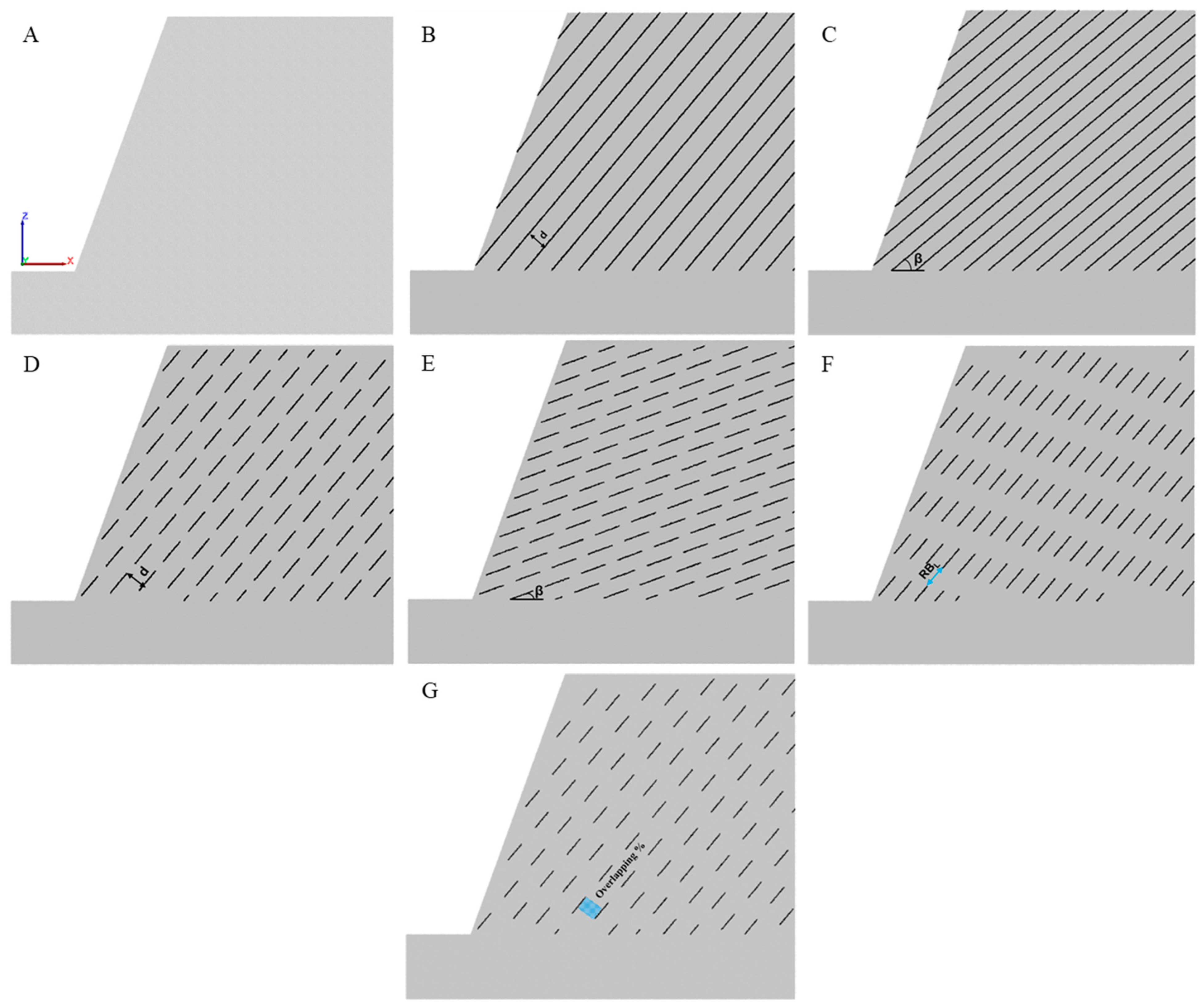
- joint spacing (d);
- joint dip angle (β);
- rock bridge length (RBL);
- overlapping joint percentages;
- joint segment length (Lj).
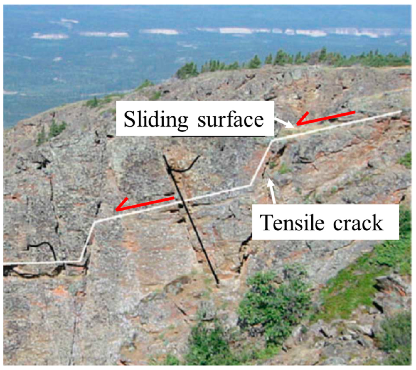
2. Persistent and Non-Persistent Discontinuities
3. Methodology
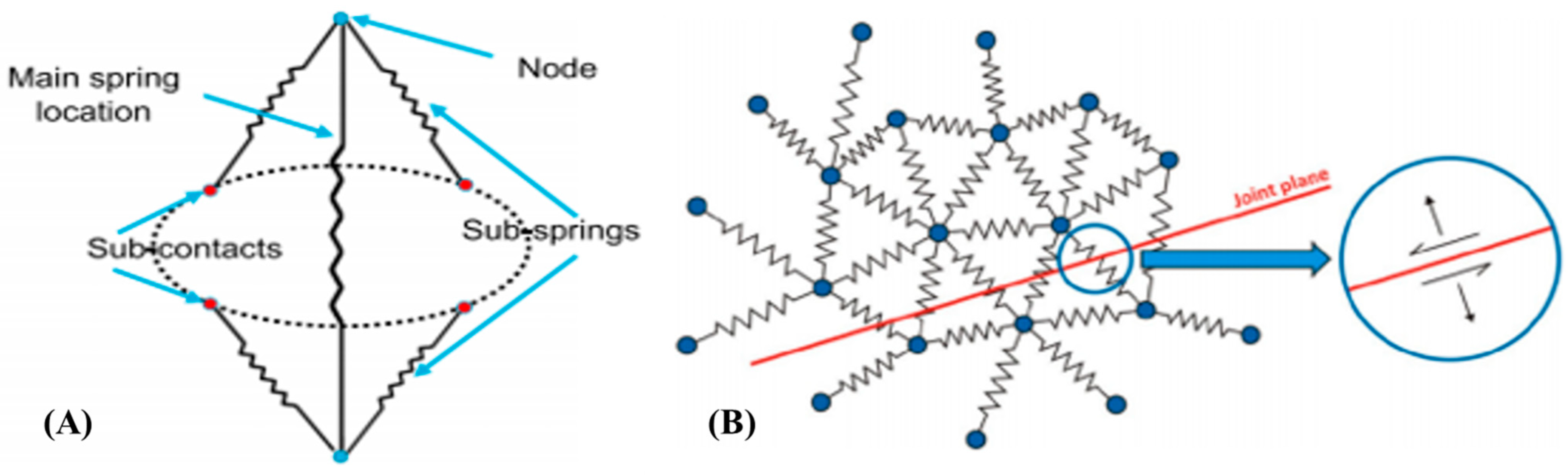
3.1. Slope Model Code
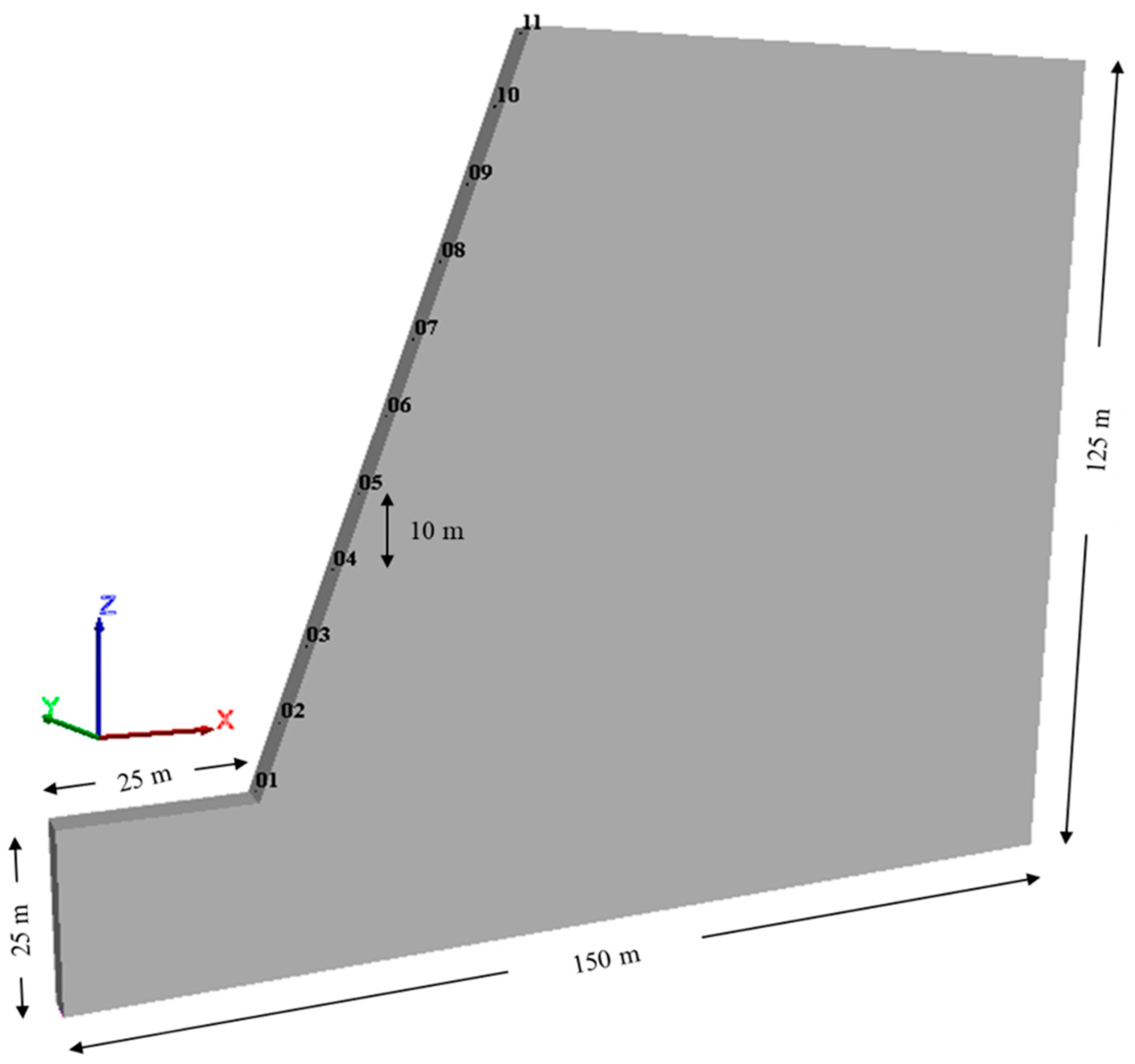
3.2. Numerical Model Set-Up
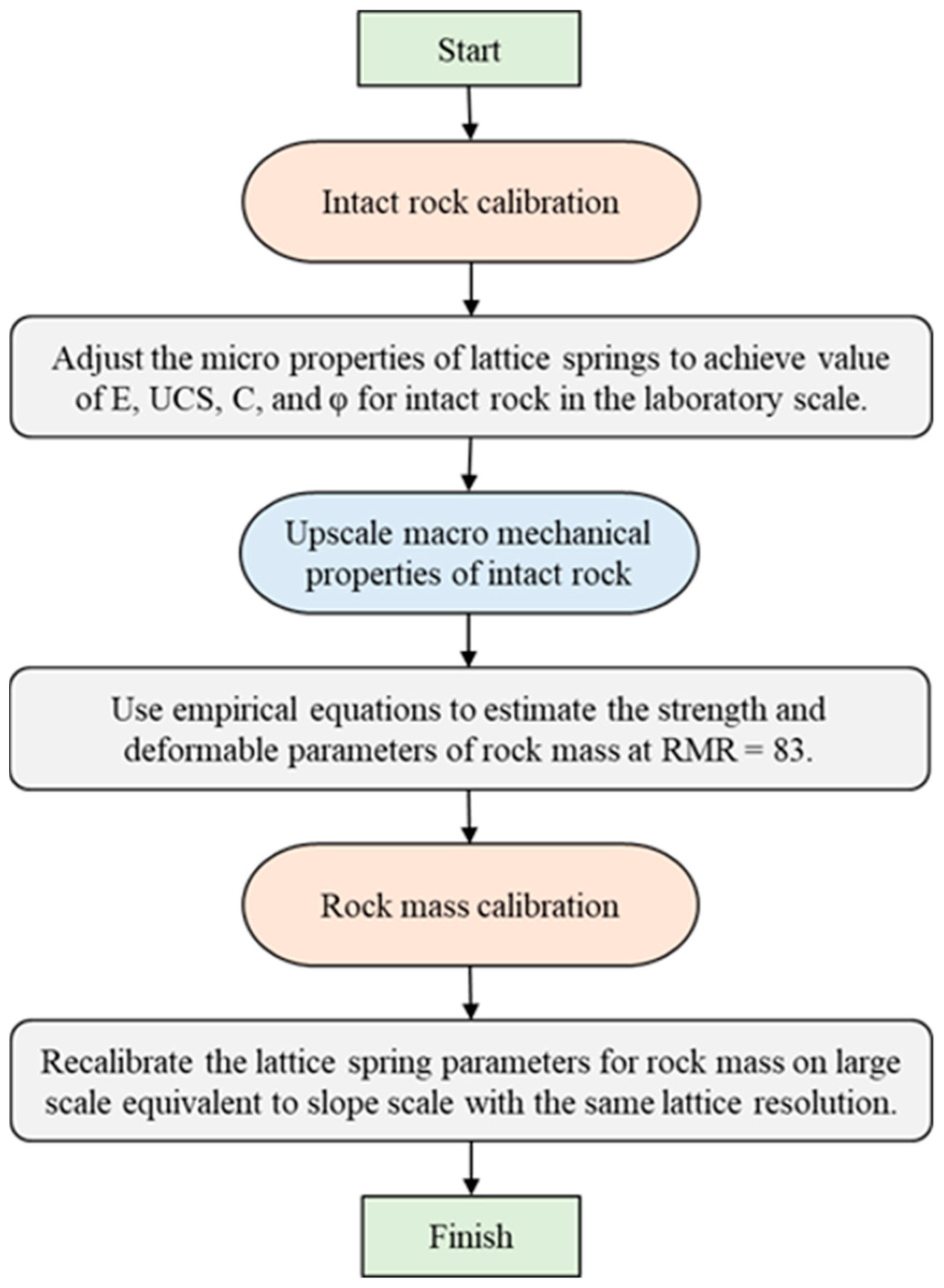
3.3. The Calibration of Micro-Scale Parameters
3.4. Strength Reduction Method
4. Parametric Studies
5. Results and Discussion
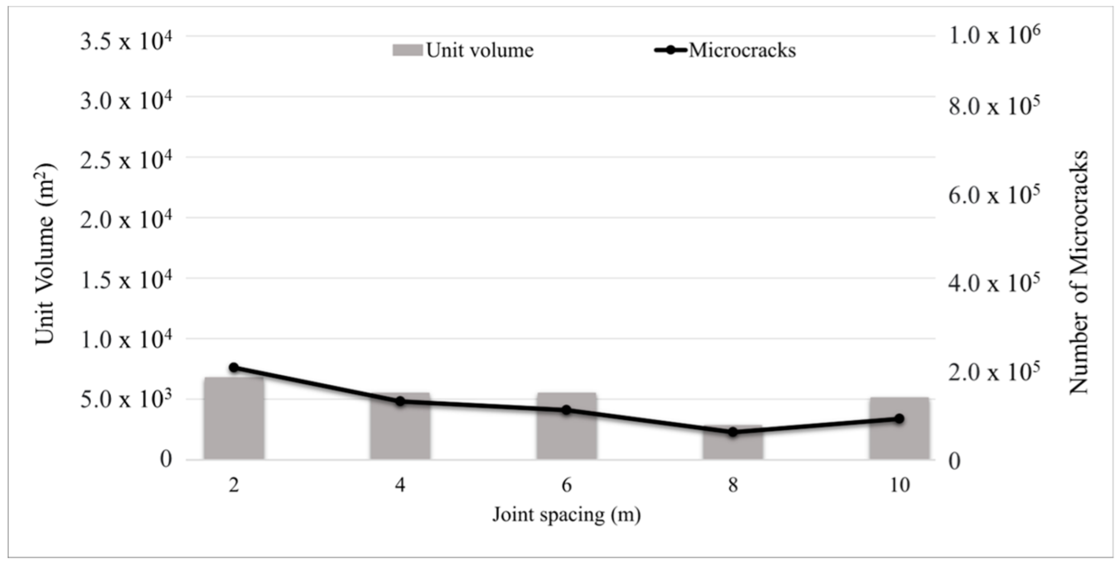
5.1. The Effect of Joint Spacing for Fully Persistent and Non-Persistent Conditions
5.1.1. Slopes Having Fully Persistent Joints
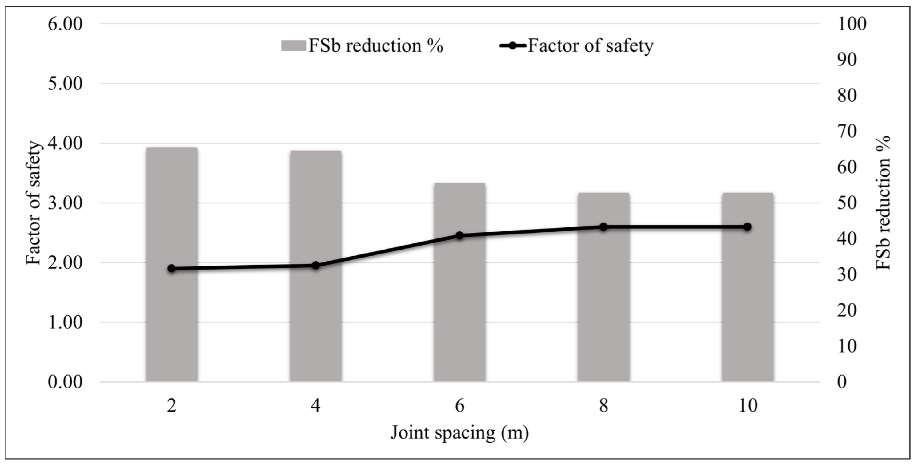
5.1.2. Slopes Having Non-Persistent Joints
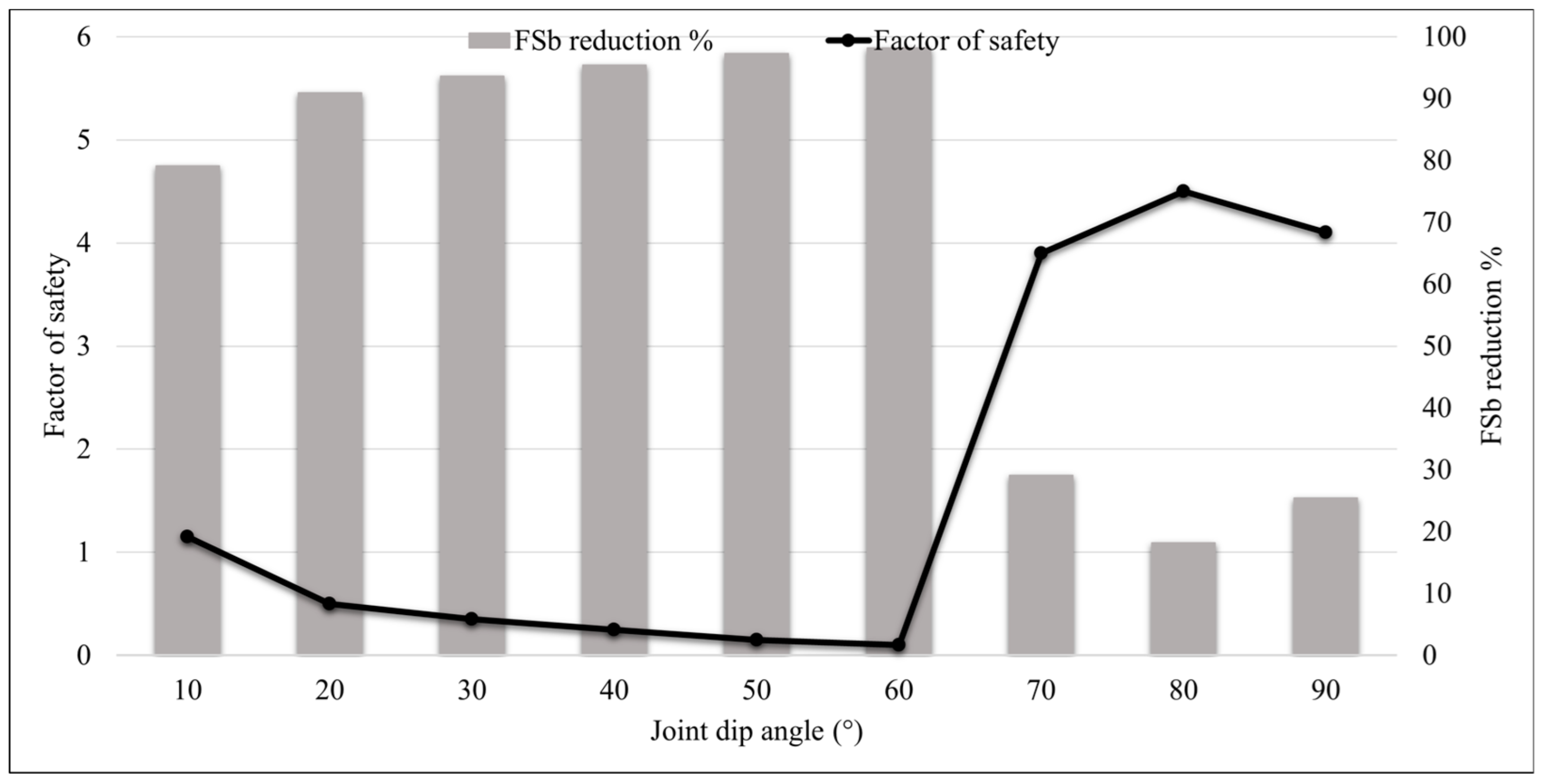
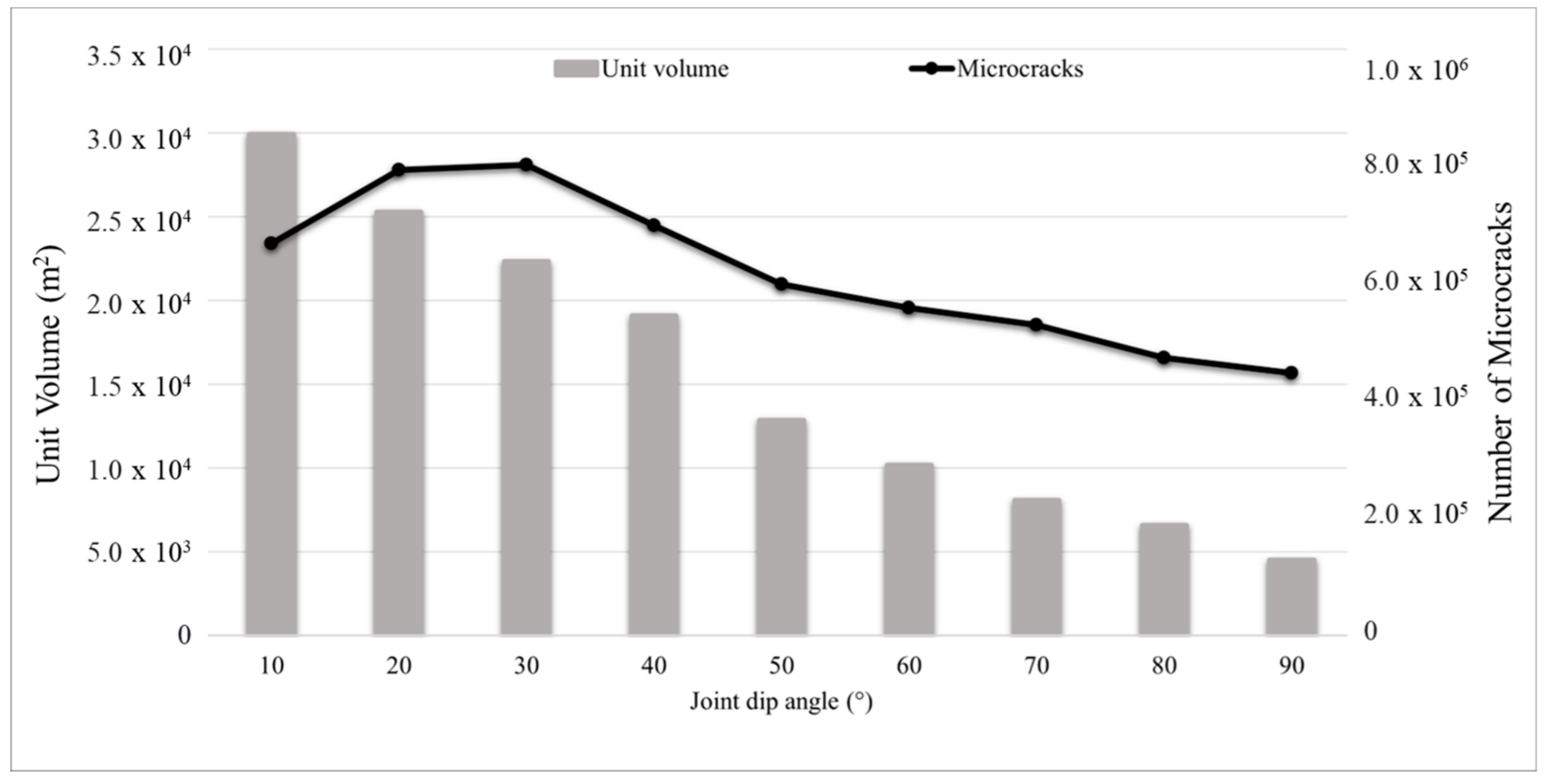
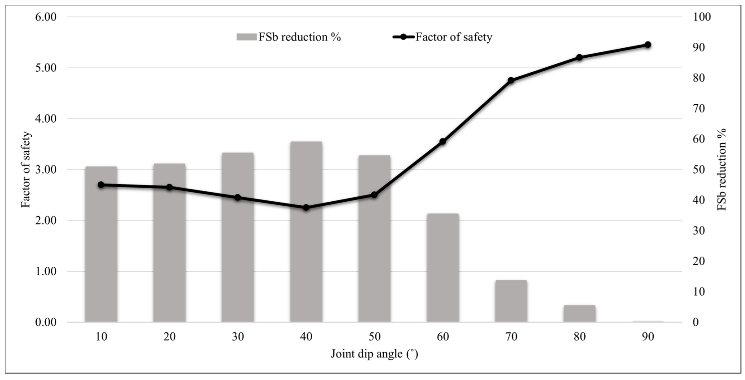
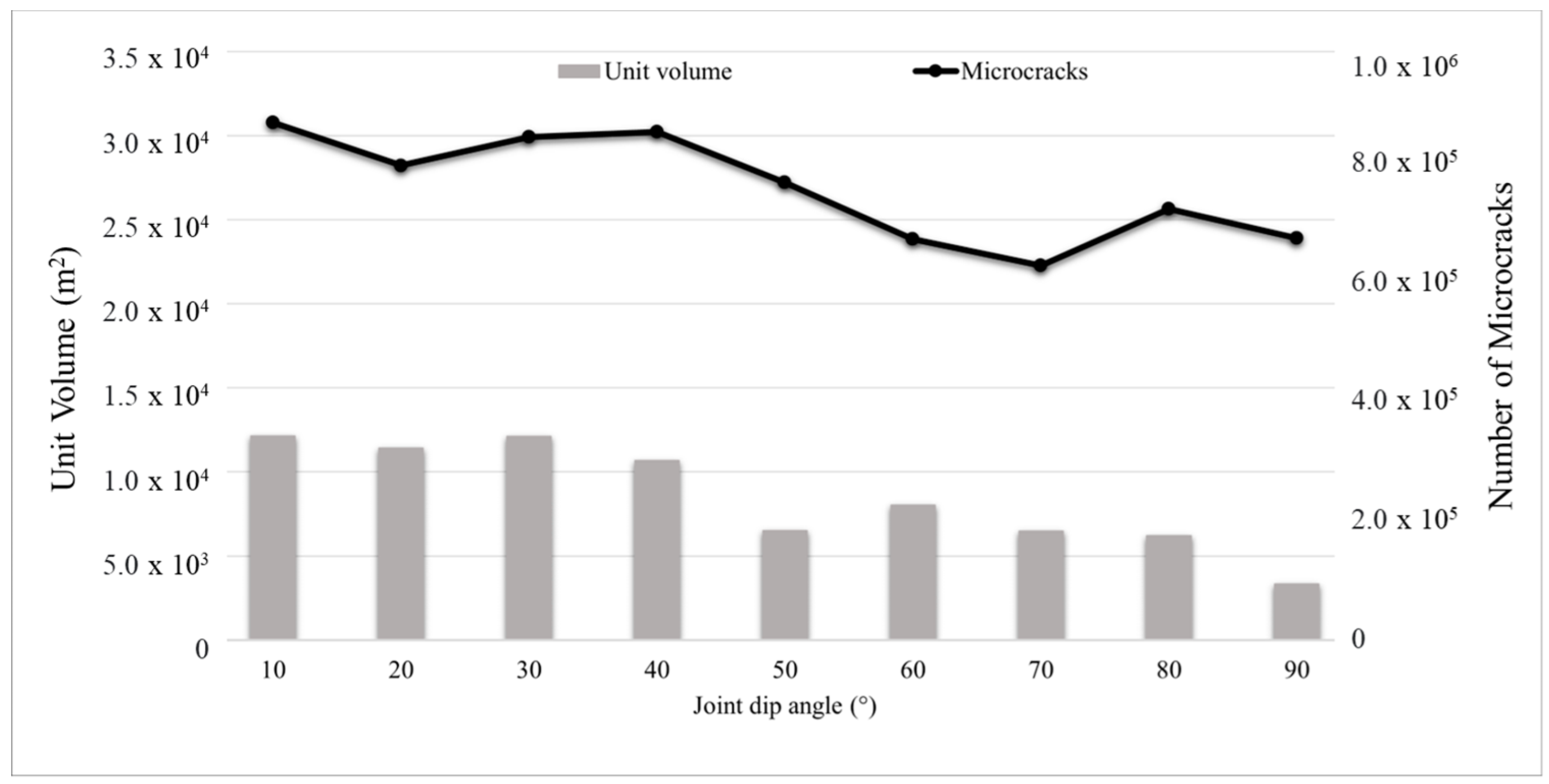
5.2. The Effect of Joint Dip Angle for Fully Persistent and Non-Persistent Conditions
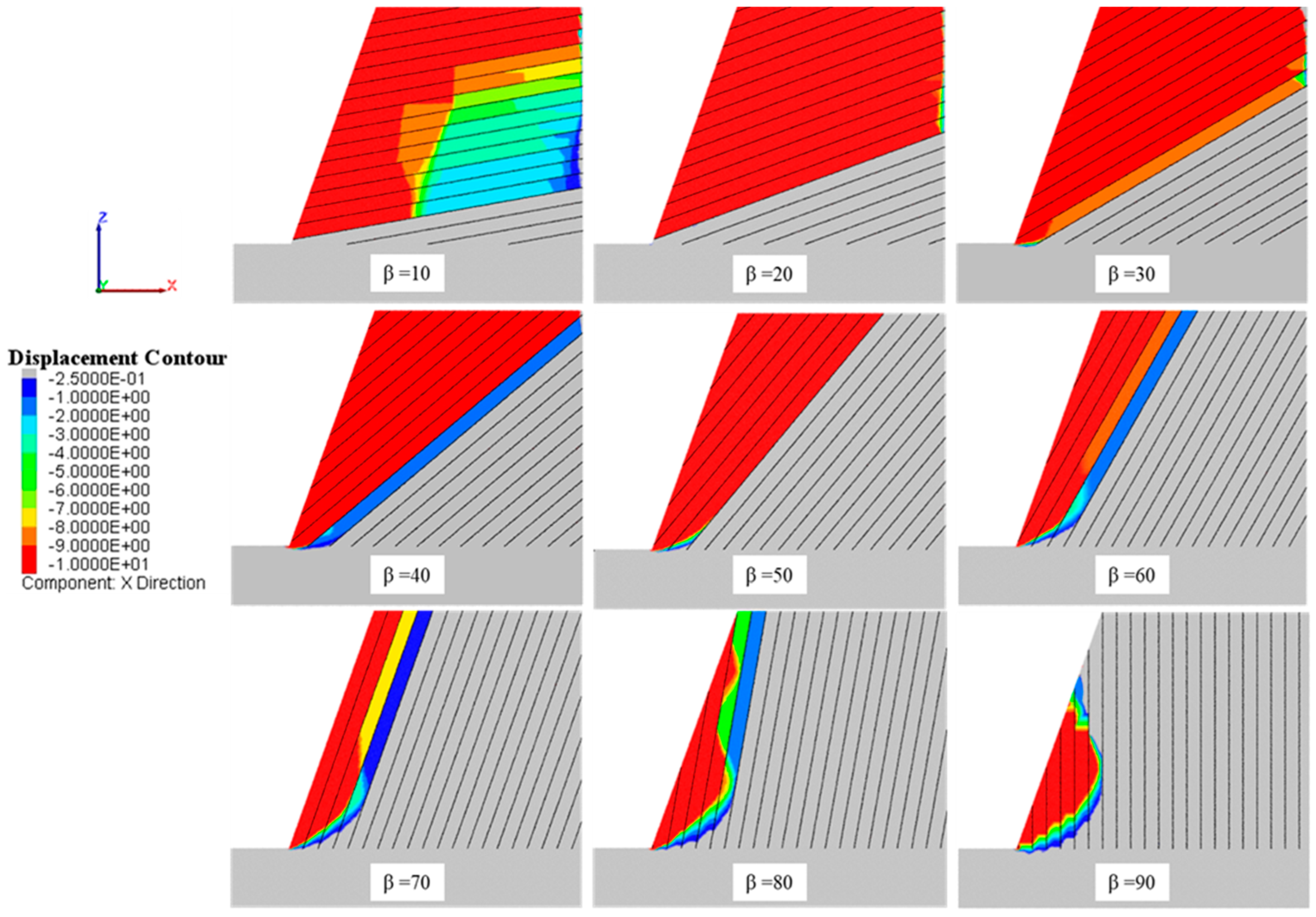
5.2.1. Slopes Having Fully Persistent Joints
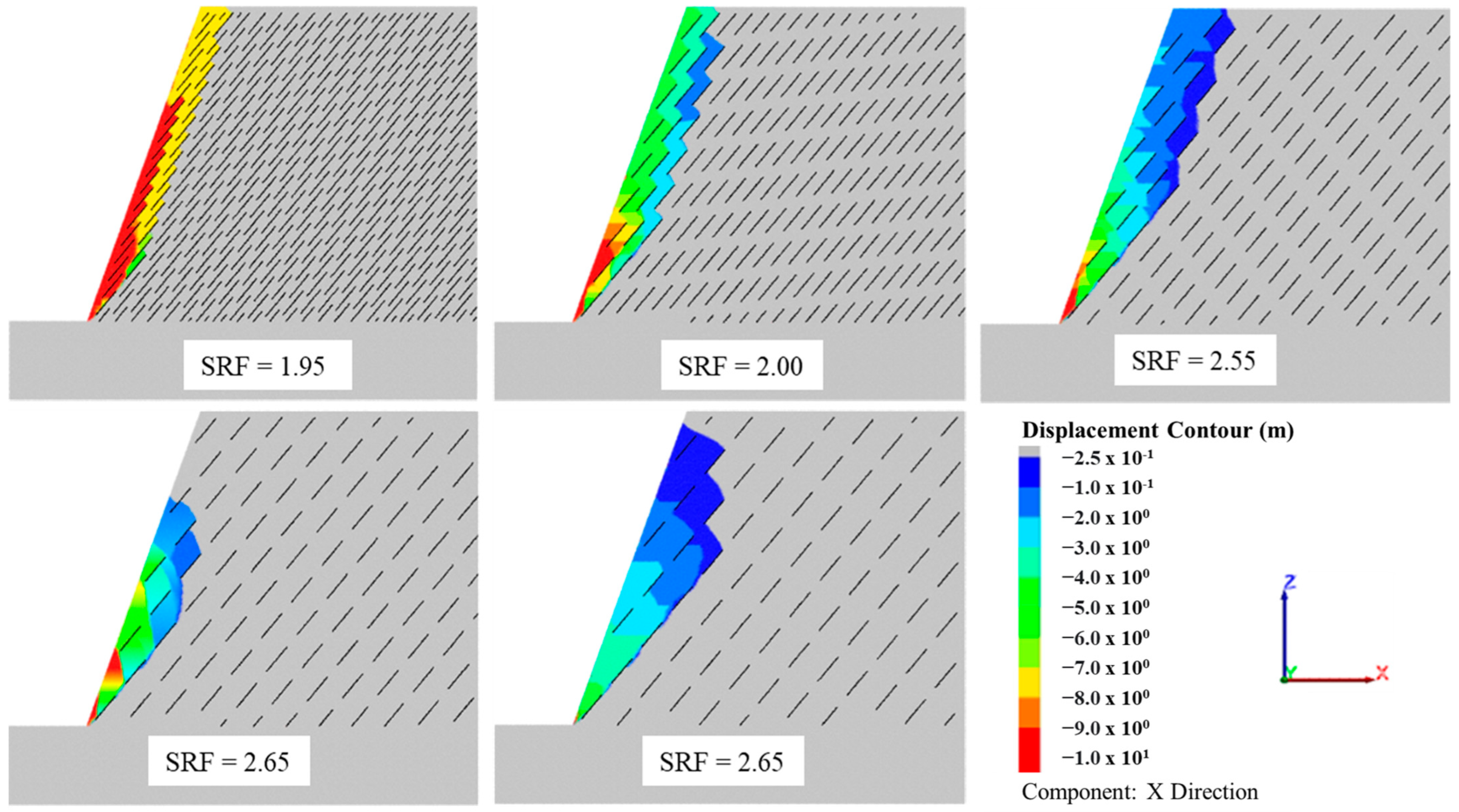
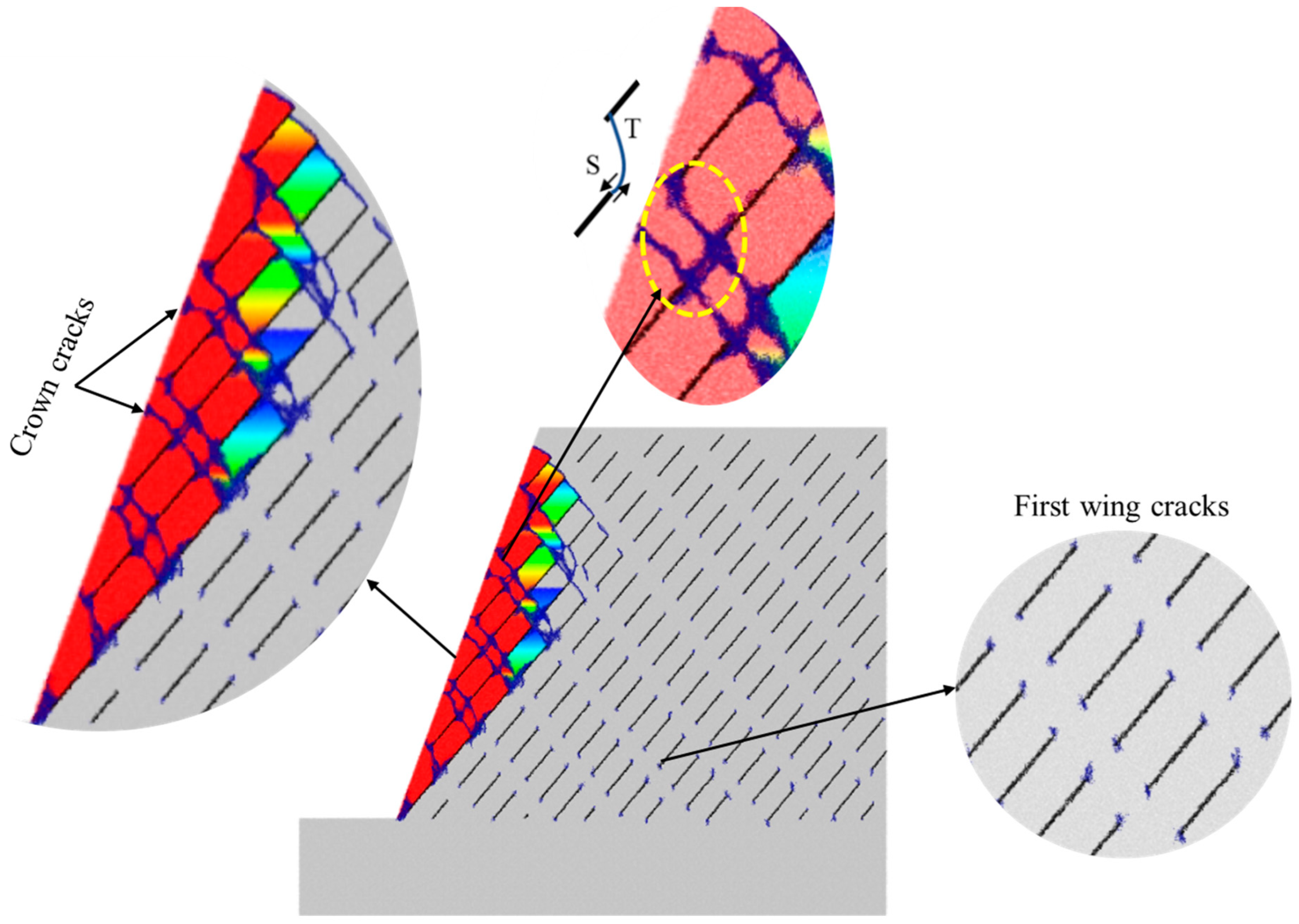
- (i)
- the blocks near the slope face are separated and slide along pre-existing joints;
- (ii)
- the subsequent blocks farther from the slope face are failed and slide along pre-existing joints, as shown in the slope with a joint dip angle of 10° in Figure 18.
5.2.2. Slopes Having Non-Persistent Joints
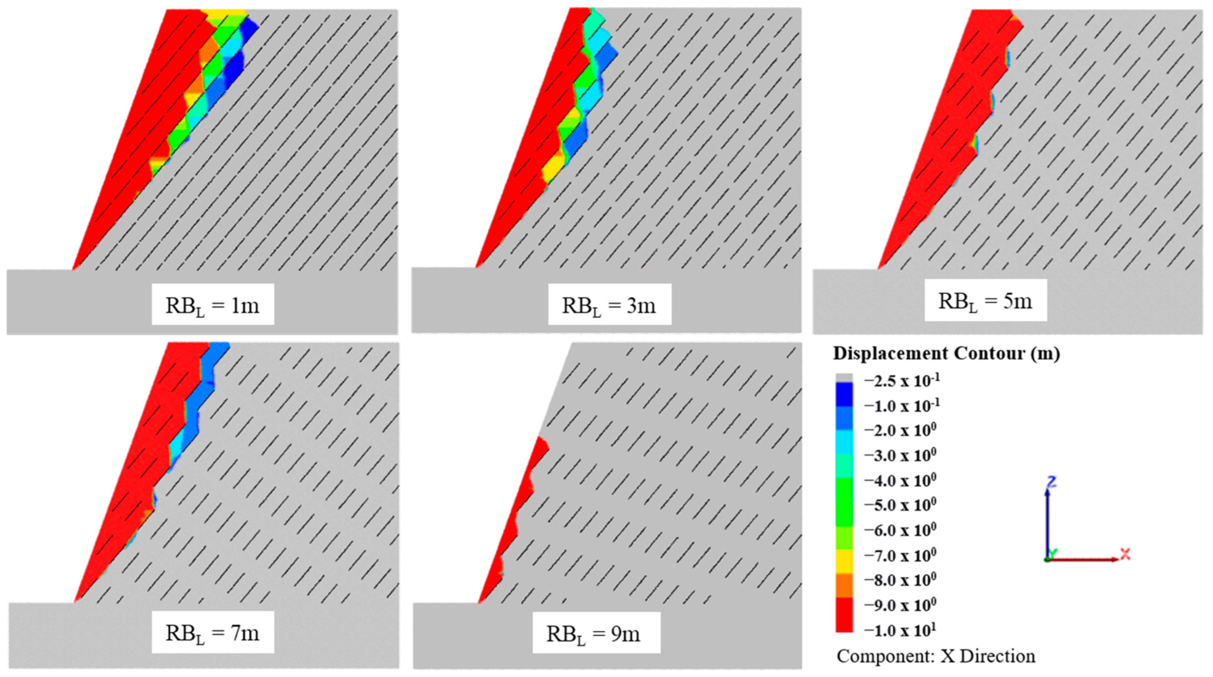
5.3. The Effect of the Rock Bridge Length and Overlapping Echelon
5.4. A Comparison of the Slopes Having Persistent and Non-Persistent Joints
6. Conclusions
Author Contributions
Funding
Institutional Review Board Statement
Informed Consent Statement
Data Availability Statement
Conflicts of Interest
References
- Deere, D.U.; Hendron, A.J.; Patton, F.D.; Cording, E.J. Design of surface and near-surface construction in rock. In Proceedings of the 8th U.S. Symposium on Rock Mechanics (USRMS), Minneapolis, MN, USA, 15–17 September 1966. [Google Scholar]
- Bieniawski, Z.T. Engineering Classification of Jointed Rock Masses. Civ. Eng. S. Afr. 1973, 15, 335–343. [Google Scholar] [CrossRef]
- Barton, N.; Lien, R.; Lunde, J. Engineering classification of rock masses for the design of tunnel support. Rock Mech. 1974, 6, 189–236. [Google Scholar] [CrossRef]
- Palmstrøm, A. Characterizing rock masses by the RMi for Use in Practical Rock Engineering: Part 1: The development of the Rock Mass index (RMi). Tunn. Undergr. Space Technol. 1996, 11, 175–188. [Google Scholar] [CrossRef]
- Hoek, E. Strength of rock and rock masses. ISRM New J. 1994, 2, 4–16. [Google Scholar]
- Zhang, L.; Einstein, H.H. Using RQD to estimate the deformation modulus of rock masses. Int. J. Rock Mech. Min. Sci. 2004, 41, 337–341. [Google Scholar] [CrossRef]
- Scholtès, L.U.C.; Donzé, F.V. Modelling progressive failure in fractured rock masses using a 3D discrete element method. Int. J. Rock Mech. Min. Sci. 2012, 52, 18–30. [Google Scholar] [CrossRef]
- Sarfaraz, H.; Amini, M. Numerical simulation of slide-toe-toppling failure using distinct element method and finite element method. Geotech. Geol. Eng. 2020, 38, 2199–2212. [Google Scholar] [CrossRef]
- Havaej, M.; Wolter, A.; Stead, D.; Tuckey, Z.; Lorig, L.; Eberhardt, E. Incorporating brittle fracture into three-dimensional modelling of rock slopes. In Proceedings of the 2013 International Symposium on Slope Stability in Open Pit Mining and Civil Engineering, Brisbane, QLD, Australia, 25–27 September 2013; Australian Centre for Geomechanics: Crawley, WA, Australia, 2013; pp. 625–638. [Google Scholar] [CrossRef]
- Tuckey, Z.S. An Integrated Field Mapping-Numerical Modelling Approach to Characterising Discontinuity Persistence and Intact Rock Bridges in Large Open Pit Slopes. Ph.D. Dissertation, Department of Earth Sciences, Simon Fraser University Science, Burnaby, Canada, 2012. [Google Scholar]
- Lian, J.J.; Li, Q.; Deng, X.F.; Zhao, G.F.; Chen, Z.Y. A Numerical Study on Toppling Failure of a Jointed Rock Slope by Using the Distinct Lattice Spring Model. Rock. Mech. Rock. Eng. 2018, 51, 513–530. [Google Scholar] [CrossRef]
- Zhao, G.F. Modelling 3D jointed rock masses using a lattice spring model. Int. J. Rock Mech. Min. Sci. 2015, 78, 79–90. [Google Scholar] [CrossRef]
- Camones, L.A.M.; Vargas, E.A.; De Figueiredo, R.P.; Velloso, R.Q. Application of the discrete element method for modeling of rock crack propagation and coalescence in the step-path failure mechanism. Eng. Geol. 2013, 153, 80–94. [Google Scholar] [CrossRef]
- Yang, S.Q.; Jiang, Y.Z.; Xu, W.Y.; Chen, X.Q. Experimental investigation on strength and failure behavior of pre-cracked marble under conventional triaxial compression. Int. J. Solids Struct. 2008, 45, 4796–4819. [Google Scholar] [CrossRef]
- Diederichs, M.S. Manuel Rocha medal recipient: Rock fracture and collapse under low confinement conditions. Rock. Mech. Rock. Eng. 2003, 36, 339–381. [Google Scholar] [CrossRef]
- Al-E’Bayat, M.; Sunkpal, M.; Sherizadeh, T. Numerical investigation of rock bridge effect on slope stability using Bonded Block Modeling method. In Proceedings of the 54th U.S. Rock Mechanics/Geomechanics Symposium, Golden, CO, USA, 28 June–1 July 2020. [Google Scholar]
- Deiminiat, A.; Aubertin, J.D.; Ethier, Y. On the calibration of a shear stress criterion for rock joints to represent the full stress-strain profile. J. Rock Mech. Geotech. Eng. 2023. [Google Scholar] [CrossRef]
- Zhao, H.; Li, S.; Zang, X.; Liu, X.; Zhang, L.; Ren, J. Uncertainty quantification of inverse analysis for geomaterials using probabilistic programming. J. Rock Mech. Geotech. Eng. 2023. [Google Scholar] [CrossRef]
- Zhou, Z.; Li, D.Q.; Xiao, T.; Cao, Z.J.; Du, W. Response surface guided adaptive slope reliability analysis in spatially varying soils. Comput. Geotech. 2021, 132, 103966. [Google Scholar] [CrossRef]
- Bastola, S.; Cai, M. Simulation of Stress-Strain Relations of Zhenping Marble Using Lattice-Spring-Based Synthetic Rock Mass Models. In Proceedings of the 52nd US Rock Mechanics/Geomechanics Symposium, Seattle, WA, USA, 17–20 June 2018. [Google Scholar]
- Manouchehrian, A.; Marji, M.F. Numerical analysis of confinement effect on crack propagation mechanism from a flaw in a pre-cracked rock under compression. Acta Mech. Sin./Lixue Xuebao 2012, 28, 1389–1397. [Google Scholar] [CrossRef]
- Park, C.H.; Bobet, A. Crack initiation, propagation and coalescence from frictional flaws in uniaxial compression. Eng. Fract. Mech. 2010, 77, 2727–2748. [Google Scholar] [CrossRef]
- Wong, L.N.Y.; Einstein, H.H. Crack coalescence in molded gypsum and carrara marble: Part 1. macroscopic observations and interpretation. Rock. Mech. Rock. Eng. 2009, 42, 475–511. [Google Scholar] [CrossRef]
- Yin, P.; Wong, R.H.C.; Chau, K.T. Coalescence of two parallel pre-existing surface cracks in granite. Int. J. Rock Mech. Min. Sci. 2014, 68, 66–84. [Google Scholar] [CrossRef]
- Zhou, X.P.; Cheng, H.; Feng, Y.F. An experimental study of crack coalescence behaviour in rock-like materials containing multiple flaws under uniaxial compression. Rock Mech. Rock Eng. 2014, 47, 1961–1986. [Google Scholar] [CrossRef]
- Jennings, J.E. A mathematical theory for the calculation of the stability of slopes in open cast mines. Plan. Open Pit Mines Proc.Johannesbg. 1970, 21, 87–102. [Google Scholar]
- Terzaghi, K. Stability of steep slopes on hard unweathered rock. Geotechnique 1962, 12, 251–270. [Google Scholar] [CrossRef]
- Einstein, H.H.; Veneziano, D.; Baecher, G.B.; O’Reilly, K.J. The effect of discontinuity persistence on rock slope stability. Int. J. Rock Mech. Min. Sci. 1983, 20, 227–236. [Google Scholar] [CrossRef]
- Zhao, G.; Wang, L.; Zhao, N.; Yang, J.; Li, X. Analysis of the variation of friction coefficient of sandstone joint in sliding. Adv. Civil. Eng. 2020, 2020, 1–12. [Google Scholar] [CrossRef]
- Damjanac, B.; Gil, I.; Pierce, M.; Sanchez, M.; Van, A.A.; McLennan, J. A new approach to hydraulic fracturing modeling in naturally fractured reservoirs. In Proceedings of the 44th US Rock Mechanics Symposium and 5th US-Canada Rock Mechanics Symposium, Salt Lake City, UT, USA, 27–30 June 2010. [Google Scholar]
- Pierce, M.; Cundall, P.; Potyondy, D.; Ivars, M.D. A synthetic rock mass model for jointed rock. In Proceedings of the 1st Canada-US Rock Mechanics Symposium-Rock Mechanics Meeting Society’s Challenges and Demands, Vancouver, BC, Canada, 27–31 May2007; Volume 1, pp. 341–349. [Google Scholar] [CrossRef]
- Lorig, L.J.; Cundall, P.A.; Damjanac, B.; Emam, S. A three-dimensional model for rock slopes based on micromechanics. In Proceedings of the 44th US Rock Mechanics Symposium and 5th US-Canada Rock Mechanics Symposium, Salt Lake City, UT, USA, 27–30 June 2010. [Google Scholar]
- Cundall, P.A.; Damjanac, B. Considerations on slope stability in a jointed rock mass. In Proceedings of the 50th US Rock Mechanics/Geomechanics Symposium, Houston, TX, USA, 26–29 June 2016. [Google Scholar]
- Zhang, W.; Wang, J.; Xu, P.; Lou, J.; Shan, B.; Wang, F.; Que, J. Stability evaluation and potential failure process of rock slopes characterized by non-persistent fractures. Nat. Hazards Earth Syst. Sci. 2020, 20, 2921–2935. [Google Scholar] [CrossRef]
- Cundall, P.A. Lattice method for modeling brittle, jointed rock. In Proceedings of the 2nd Int’l FLAC/DEM Symposium on Continuum and Distinct Element Numerical Modeling in Geomechanics, Melbourne, Australia, 14–16 February 2011. [Google Scholar]
- Itasca. SRMTools-User’s Guide and Tutorial; Itasca Consulting Group, Inc.: Minneapolis, MN, USA, 2017. [Google Scholar]
- Sainsbury, D.; Pothitos, F.; Finn, D.; Silva, R. Three-dimensional discontinuum analysis of structurally controlled failure mechanisms at the cadia hill open pit. In Proceedings of the 2007 International Symposium on Rock Slope Stability in Open Pit Mining and Civil Engineering, Perth, Australia, 12–14 September 2007; Australian Centre for Geomechanics: Crawley, WA, Australia, 2007; pp. 307–320. [Google Scholar] [CrossRef]
- Patel, M.B.; Shah, M.V. Strength characteristics for limestone and dolomite rock matrix using tri-axial system. IJSTE—Int. J. Sci. Technol. Eng. 2015, 1, 114–124. [Google Scholar]
- Bastola, S.; Cai, M. Investigation of mechanical properties and crack propagation in pre-cracked marbles using lattice-spring-based synthetic rock mass (LS-SRM) modeling approach. Comput. Geotech. 2019, 110, 28–43. [Google Scholar] [CrossRef]
- Al-E’Bayat, M.; Sherizadeh, T.; Guner, D.; Asadizadeh, M. Lattice-spring-based synthetic rock mass model calibration using response surface methodology. Geomech. Eng. 2022, 31, 529–543. [Google Scholar] [CrossRef]
- Al-E’Bayat, M.; Sherizadeh, T.; Guner, D. Laboratory-Scale Investigation on Shear Behavior of Non-Persistent Joints and Joint Infill Using Lattice-Spring-Based Synthetic Rock Mass Model. Geosciences 2023, 13, 23. [Google Scholar] [CrossRef]
- Lajtai, E.Z. Brittle fracture in compression. Int. J. Fract. 1974, 10, 525–536. [Google Scholar] [CrossRef]
- Ramamurthy, T. A geo-engineering classification for rocks and rock masses. Int. J. Rock Mech. Min. Sci. 2004, 41, 89–101. [Google Scholar] [CrossRef]
- Zienkiewicz, O.C.; Humpheson, C.; Lewis, R.W. Associated and non-associated visco-plasticity and plasticity in soil mechanics. Geotechnique 1975, 25, 671–689. [Google Scholar] [CrossRef]
- Cheng, Y.M.; Lansivaara, T.; Wei, W.B. Two-dimensional slope stability analysis by limit equilibrium and strength reduction methods. Comput. Geotech. 2007, 34, 137–150. [Google Scholar] [CrossRef]
- Dawson, E.M.; Roth, W.H.; Drescher, A. Slope stability analysis by strength reduction. Geotechnique 1999, 49, 835–840. [Google Scholar] [CrossRef]
- Hammah, R.E.; Yacoub, T.; Corkum, B.; Wibowo, F.; Curran, J.H. Analysis of blocky rock slopes with finite element shear strength reduction analysis. In Proceedings of the 1st Canada-US Rock Mechanics Symposium, Vancouver, BC, Canada, 27–31 May 2007. [Google Scholar]
- Seyed-Kolbadi, S.M.; Sadoghi-Yazdi, J.; Hariri-Ardebili, M.A. An improved strength reduction-based slope stability analysis. Geosciences 2019, 9, 55. [Google Scholar] [CrossRef]
- Zheng, B.; Qi, S.; Guo, S.; Huang, X.; Liang, N.; Zou, Y.; Luo, G. A new shear strength criterion for rock masses with non-persistent discontinuities considering the nonlinear progressive failure process. Materials 2020, 13, 4694. [Google Scholar] [CrossRef]
- Hoek, E.; Bray, J.D. Rock Slope Engineering; CRC press: Boca Raton, FL, USA, 1981. [Google Scholar]
- Huang, D.; Cen, D.; Ma, G.; Huang, R. Step-path failure of rock slopes with intermittent joints. Landslides 2015, 12, 911–926. [Google Scholar] [CrossRef]
- Zhang, L. Engineering Properties of Rocks; Butterworth-Heinemann: Kidlington, UK; Elsevier: Amsterdam, The Netherlands, 2016; 304p. [Google Scholar]


| Intact Rock Properties | Unit | Value |
|---|---|---|
| Density | kg/m3 | 2125 |
| Young’s modulus | GPa | 1.27 |
| Poisson’s ratio | - | 0.22 |
| Compressive strength | MPa | 29.05 |
| Tensile strength | MPa | 2.9 |
| Friction | degree | 26 |
| Cohesion | MPa | 7.3 |
| Intact Rock Properties | Unit | Micro | Macro |
|---|---|---|---|
| Young’s modulus | GPa | 0.18 | 1.26 |
| Uniaxial compressive strength | MPa | 21.4 | 26.50 |
| Tensile strength | MPa | 2.9 | 2.9 |
| Peak friction of flat joint | degree | 40 | 27.4 |
| Residual friction of flat joint | degree | 0 | 0 |
| Radius multiplier | - | 0.9 | 0.9 |
| Rock Mass Properties | Unit | Empirical | Numerical | Error (%) |
|---|---|---|---|---|
| Young’s modulus | GPa | 0.040 | 0.043 | 7 |
| Uniaxial compressive strength | MPa | 14.69 | 14.63 | 0 |
| Persistent Joint Parameters | Values | |
| Group A | Base case | No joint |
| Group B | Joint spacing (m) | 2, 4, 6, 8, & 10 |
| Group C | Joint dip angle (°) | 10, 20, 30, …, & 90 |
| Non-Persistent Joint Parameters | Values | |
| Group D | Joint spacing (m) | 2, 4, 6, 8, & 10 |
| Group E | Joint dip angle (°) | 10, 20, 30, …, & 90 |
| Group F | Rock bridge length (m) | 1, 3, 5, 7, & 9 |
| Group G | Joint overlapping (%) | 0, 50, & 100 |
Disclaimer/Publisher’s Note: The statements, opinions and data contained in all publications are solely those of the individual author(s) and contributor(s) and not of MDPI and/or the editor(s). MDPI and/or the editor(s) disclaim responsibility for any injury to people or property resulting from any ideas, methods, instructions or products referred to in the content. |
© 2024 by the authors. Licensee MDPI, Basel, Switzerland. This article is an open access article distributed under the terms and conditions of the Creative Commons Attribution (CC BY) license (https://creativecommons.org/licenses/by/4.0/).
Share and Cite
Al-E’Bayat, M.; Guner, D.; Sherizadeh, T.; Asadizadeh, M. Numerical Investigation for the Effect of Joint Persistence on Rock Slope Stability Using a Lattice Spring-Based Synthetic Rock Mass Model. Sustainability 2024, 16, 894. https://doi.org/10.3390/su16020894
Al-E’Bayat M, Guner D, Sherizadeh T, Asadizadeh M. Numerical Investigation for the Effect of Joint Persistence on Rock Slope Stability Using a Lattice Spring-Based Synthetic Rock Mass Model. Sustainability. 2024; 16(2):894. https://doi.org/10.3390/su16020894
Chicago/Turabian StyleAl-E’Bayat, Mariam, Dogukan Guner, Taghi Sherizadeh, and Mostafa Asadizadeh. 2024. "Numerical Investigation for the Effect of Joint Persistence on Rock Slope Stability Using a Lattice Spring-Based Synthetic Rock Mass Model" Sustainability 16, no. 2: 894. https://doi.org/10.3390/su16020894