Demand Response Strategy Based on the Multi-Agent System and Multiple-Load Participation

Abstract

In order to improve the utilization of user-side power resources in the distribution network and promote energy conservation, this paper designs a distributed system suitable for power demand response (DR), considering multi-agent system (MAS) technology and consistency algorithms. Due to the frequent changes in the power system structure caused by changes in the load of a large number of users, this paper proposes using cluster partitioning indicators as communication weights between agents, enabling agents to utilize the distribution network for collaborative optimization. In order to achieve the integration of multiple load-side power resources and improve the refinement level of demand-side management (DSM), two types of agents with load aggregator (LA) functions are provided, which adopt the demand response strategies of Time-of-Use (TOU) or Direct Load Control (DLC) and model the uncertainty of individual device states using Monte Carlo method, so that the two typical flexible loads can achieve the target load-reduction requirements under the MAS framework. The research results demonstrate that this method achieves complementary advantages of the two types of loads participating in DR on a time scale, reducing the costs of power companies and saving customers’ electricity bills while peak shaving.

1. Introduction

The rapid development of the new energy industry has caused difficulties in consuming wind and solar power in the power grid, as well as problems such as waste of power resources [1]. At the same time, the increase in peak electricity consumption and the complexity of electricity loads have led to an insufficient utilization of resources for electricity consumers. With the advancement of smart grid (SG) technology, the concept of power producers has been expanded [2]; in recent years, there has been a growth in studies focusing on the active support of typical loads on the user side for power grid stability, such as electric water heaters, air conditioners (ACs), electric vehicles (EVs), etc. [3,4]. These loads are called flexible loads, and their capacity is small and distributed dispersedly. Usually, an aggregation model needs to be established and used in the form of a load aggregator (LA) to participate in the fields of solar and wind power consumption, demand response (DR), and so on [5]. However, these power resources have different types and characteristics, making it difficult to coordinate them effectively.

The traditional LA participation in power dispatch is still in a centralized framework, which is not well-matched with the time-varying characteristics of flexible loads [6], for example, predicting market prices to characterize the uncertainty of electric vehicle LAs, and then optimizing the scheduling of EVs through the constraints of electric vehicle operation and vehicle access to the grid [7]. Introducing LAs helps maintain the independence and autonomy of the park under centralized and unified scheduling. LAs can serve as a link between users and the integrated demand response (IDR) market in the park, improving economic efficiency and exploring user demand response capabilities [8]. LAs can also be combined with some intelligent algorithms; for example, when evaluating and classifying virtual power plants (VPPs) facing DR, the AdaBoost algorithm can be combined with backpropagation (BP) neural networks to measure the DR effect of VPPs [9]. In terms of demand-side management (DSM), LAs can use different artificial intelligence technologies to prioritize DR devices for users; reference [10] uses k-means clustering technology to determine user comfort, uses genetic algorithm to solve the balance problem between energy cost and user comfort, and uses support vector regression technology for numerical simulation verification. These studies generally face the problem of single-load types and weak universality, and some intelligent algorithms suitable for LAs with multiple loads require relatively high hardware requirements.

The centralized control system usually adopts a fixed scheduling mode, which first comprehensively evaluates the priority of the LA, considers power contribution and confidence, etc. As the number and types of LAs increase, it is often necessary for the system to re-plan the LA or reconstruct multi-layer game systems, and it cannot effectively handle the structural changes of the power system [11]. Therefore, adopting distributed control is currently the key to achieving an effective utilization of LA resources. The development of multi-agent systems (MASs) and related technologies meets the control requirements for these power resources [12]. The concept of MASs is relatively mature in the field of artificial intelligence [13]. Multi-agent systems can divide complex systems into multiple agents that can operate autonomously and communicate with each other. Through coordinated control between agents, distributed system optimization problems that traditional centralized systems cannot effectively solve can be solved, which can improve the problem processing speed and real-time system performance.

At present, the concept of the MAS has also been applied in the field of smart grids (SGs), and researchers are exploring its widespread application in this field. In SGs, MAS-based methods help achieve system control, information processing, participation in market competition, analysis of electricity consumer behavior, and agent-based decision support [14]. Reference [15] proposed a new scheduling strategy based on the combination of evolutionary game theory (EGT) and particle swarm optimization (PSO) within the MAS framework, which rewards the agent for stabilizing the voltage distribution in the distribution network, obtains the optimal scheduling, and can manage the voltage distribution. Moreover, due to the characteristics of the MAS, it has shown impressive performance in DR in residential and industrial parks. Reference [16] proposes an MAS suitable for solving the optimal residential DR, where the agents are divided into heterogeneous home agents (HA) and retailer agents (RA), and incorporates load forecasting and price forecasting. The real-time pricing (RTP) DR strategy is used to assist homeowners in formulating electricity consumption plans. Reference [17] proposes an MAS based on an existing Virtual Power Plant (VPP) system, which is suitable for the interface of standard equipment in industrial parks, helping industrial parks provide flexibility in actual DR in order to address the highly abstract issues of existing MAS research in DR. Some studies on the MAS framework for specific load types participating in DR have shown the application of MASs in distributed control. When using direct load control for air conditioner loads, the temperature rises and varies change, and the MAS is used to balance the differences in individual device control effects [18].

However, there have been few studies that have developed agents with LA functionality under the MAS framework, as various types of loads lack the ability to communicate with each other, making it difficult for agents to handle the output or priority balancing problems of multiple loads and failing to fully utilize the potential of the load side to jointly solve demand response and other problems [19]. Moreover, facing MASs with complex connection relationships between agents, it is difficult to establish a model and handle an MAS with a black-box state.

Based on the above background and considering flexibility, this paper proposes an LA control method that does not rely on a centralized control system. A multi-agent system (MAS) is designed, which analyzes the incentive compensation of power grid companies for users, uses incremental costs and quantified LA demand response ability as communication information between agents, and connects agents through consistency algorithms. Compared with traditional agents that participate in DR based on priority, the MAS improves the demand response value of low-DR-cost agents and reduces the demand response value of high-DR-cost agents. Furthermore, based on consistency algorithms, this article uses electrical distance in cluster partitioning indicators as communication weights between agents and establishes a layered multi-agent system, constrained by the system power balance and the upper and lower limits of the adjustable capacity of the agents. Compared to traditional MASs, this method is suitable for distribution network structures; especially in situations where the communication relationship between agents is unknown, connections can be established through electrical relationships. Finally, this article analyzes the changes and related characteristics of each agent in DR scenarios.

If the LA lacks specific model support and does not specify different control methods for the LA, it will reduce its universality. However, in existing studies, most LA models involved in DR have not clearly defined the type of individual load devices, which is crucial for achieving load control during the DR process [20]. This article establishes models for the loads under two typical DR strategies, starting from individual devices, focusing on releasing power resources from the user side, promoting energy conservation and emission reduction, and using the Monte Carlo method for uncertainty modeling. For the air conditioner load, a Direct Load Control (DLC) strategy is adopted to obtain demand response capability, taking into account the uncertainty of the external temperature and the initial state of the air conditioner; for the load of electric vehicles, a Time-of-Use (TOU) strategy is adopted to obtain the demand response capability, taking into account the uncertainty of the user’s parking time. As the Monte Carlo approach can model the uncertainty of the research object, we adopted it in this paper.

The results indicate that this technology helps power grid operators achieve the minimum total incentive provided to consumers while meeting the power reduction goals and optimizing demand response costs. Electricity consumers can not only receive incentives, but also reduce their peak electricity consumption and save on electricity costs. The results show that these two agents are able to control individual devices excellently. Besides, the proposed method in this article is more suitable for scenarios where multiple users participate in the demand response, improving the utilization of power resources and achieving complementary advantages of multiple loads. At the same time, the corresponding LAs are supported by uncertainty models [16], making the data generated by LAs in this article more reliable.

2. MAS-Based Demand Response Strategy

2.1. Hierarchical Optimization Model for DR

In the theory related to MASs [21], the structure of MASs’ network topology is formed by the connecting routes or communication channels between agents, and each agent in the MAS can be considered as a self-regulating node [22]. In demand response, this means that agents can regulate and aggregate the characteristics of individual loads of LAs. The MAS can also use network topology to seek collaborative solutions for optimization problems, conduct joint regulation among agents, and build hierarchical optimization systems [23,24].

This article proposes a hierarchical distributed control system using MAS for demand response (DR) in the distribution network system. It is divided into a system layer, an agent layer (load aggregation layer), and an individual device layer from top to bottom. The upper two layers play the roles of the dispatch center and control center, respectively. The relationships and information to be transmitted between each layer are shown in Figure 1.

In Figure 1, the system layer is responsible for monitoring and managing the operation of the power system, including arranging power generation plans, dispatching power resources, and handling emergency situations. When the system is experiencing power shortages or needs to absorb wind and solar energy, the system layer will issue demand response tasks to the agent layer.

The agent layer is responsible for handling the collaborative solution of the objective function, enabling each agent to communicate in the system’s adjustment task in order to obtain the optimal adjustment cost of the system. The agent layer will also aggregate information from the device layer and output control instructions to the device layer.

The device layer is responsible for implementing the specific management of individual devices, executing control instructions from the agent layer, and utilizing sensors to provide load aggregation information (device operation status) to the agent layer, forming feedback.

The specific steps to establish the demand response system include establishing a flexible load aggregation model with a variable scale; proposing a demand response strategy for load aggregators, and evaluating and integrating the demand response capability of the multi-load models; by participating in the demand response through a multi-agent system, the speed and accuracy of multi-load aggregators’ joint participation in demand response tasks can be improved.

2.2. Objective Function and Constraints

The demand response objective functions and constraints to be used in the hierarchical optimization model are shown below:

$$\{\begin{array}{cc}\min & F_D={\displaystyle \sum _{i=1}^N{F}_{Di}}(P_{Di}),\forall i\in N\\ \mathrm{s}.\mathrm{t}.& {\displaystyle \sum _{i=1}^N{P}_{Di}}=\delta P_D\\ & P_{Di}^{\min }\le P_{Di}\le P_{Di}^{\max }\end{array}$$

(1)

where $F_D$ is the total cost; and $P_{Di}$ is the total power reduction for the corresponding agent.

The demand response objective functions and constraints required in the hierarchical optimization model are shown below.

For $P_{Di}$, there will be changes due to different types of power resource combinations and time $t$, and the relevant constraints of various load agents included are as follows:

(1)

Constraints on the power reduction of air conditioner loads:

$$P_{DAC,i}^{\min }(t)\le P_{DAC,i}(t)\le P_{DAC,i}^{\max }(t)$$

(2)

where $P_{DAC,i}(t)$ is the difference between the maximum power of the air conditioner aggregation and the current power, and it will change constantly with changes in external temperature.

(2)

Constraints on the power reduction of electric vehicle loads:

$$P_{DEV,i}^{\min }(t)\le P_{DEV,i}(t)\le P_{DEV,i}^{\max }(t)$$

(3)

where $P_{DEV,i}(t)$ is the difference between the aggregated maximum power and current power of electric vehicles, which has a negative correlation with their daily load curve.

(3)

Constraints applicable to distribution network structure and related power flow that meet cluster partitioning indicators:

$$\{\begin{array}{l}{P}_i(q,V)-P_{gi}+P_{di}=0\\ Q_i(q,V)-Q_{gi}+Q_{di}=0\\ V_i^{\min }\le V_i\le V_i^{\max }\\ P_j{}^{\min }\le P_j\le P_j{}^{\max }\\ Q_j{}^{\min }\le Q_j\le Q_j{}^{\max }\end{array}$$

(4)

where $P_{gi}$ and $Q_{gi}$ are the active power output and reactive power output of each node; $P_{di}$ and $Q_{di}$ are the active power demand and reactive power demand of each node; $P_i$ and $Q_i$ are constraints on the balance of the active and reactive power of nodes; $V_i$ is the constraint of bus voltage; and $P_j$ and $Q_j$ are constraints on the active and reactive outputs of the generator set equipment.

3. Strategies for Demand Respond Based on MAS

3.1. Hierarchical Optimization Model for Demand Response

The cost on the demand side for an electric company is a quadratic function of the total actual reduction in user load, and the cost of a single agent in the MAS adheres to this principle. The cost function is shown below:

$$C(P_D)=\alpha P_D^2+\beta P_D+\gamma ,\forall i\in N$$

(5)

$$F_{Di}(P_D)={\alpha }_i{P}_{Di}^2+{\beta }_i{P}_{Di}+{\gamma }_i,\forall i\in N$$

(6)

where $C$ is the demand-side cost of the power company; $P_{Di}$ is the total actual reduction of a single agent; and $F_{Di}$ is the demand response cost of a single agent.

The goal is to optimize load reduction costs. The optimization of the cost function is solved using the Lagrange relaxation method:

$$\begin{array}{l}{F}_D{}^{*}=F_D(P_{D1},P_{D2},\dots ,P_{DN})-\lambda f(P_{D1},P_{D2},\dots ,P_{DN})\\ F_D{}^{*}=(F_{D1},F_{D2},\dots ,F_{DN})-\lambda ({\displaystyle \sum _{i=1}^N{P}_{Di}-\delta P_D})\end{array}$$

(7)

Take the partial derivatives of $P_{Di}$ for each side of the equation:

$$\begin{array}{l}\frac{\partial F_D^{*}}{\partial P_{Di}}=\frac{\partial F_{Di}}{\partial P_{Di}}-\lambda =0,\forall i\in N\\ \lambda =\frac{\partial F_{Di}}{\partial P_{Di}}=\frac{d{F}_{Di}}{d{P}_{Di}},\forall i\in N\end{array}$$

(8)

where $\lambda$ is the Lagrange multiplier, representing the derivative of cost overload reduction.

The results indicate that if the partial derivative of each agent’s cost-to-power is consistent, then the total cost of the system is the lowest. This partial derivative, known as the incremental cost, is linearly related to the amount of power reduction, showing that reducing the cut power in the demand response process by an agent with a higher incremental cost can reduce the total cost.

The consistency algorithm derived from algebraic graph theory is suitable for the complex network topology of the MAS and is the fundamental method for solving MAS control problems. It achieves consistency of control information through iterative relationship matrices, and the incremental cost is first-order information, which conforms to the characteristics of iteratively solvable control information in the consistency algorithm.

In the consistency algorithm, there are the following rules for the first-order dynamic information ${\dot{x}}_i$ of communication between agents:

$${\dot{x}}_i=x_i,i=1,2,\dots ,n$$

(9)

The process of transmitting first-order dynamic information and solving consistent solutions under continuous time can be achieved by iterating the Laplace matrix [25]:

$$\begin{array}{l}{\dot{x}}_i=-{\displaystyle \sum _{j=1}^n{A}_{ij}}(x_i-x_j),i=1,2,\dots ,n,j=1,2,\dots ,n\\ \dot{x}(t)=-L(t)x(t)\\ L_{ij}\{\begin{array}{c}{\displaystyle \sum _{i\ne j}{A}_{ij},i=j,i=1,2,\dots ,n,j=1,2,\dots },n\\ -A_{ij},i\ne j,i=1,2,\dots ,n,j=1,2,\dots ,n\end{array}\end{array}$$

(10)

where $L_{ij}$ is the element in the Laplace matrix; and $A_{ij}$ is the element in the adjacency matrix.

Assign values based on communication weights. In practical situations, due to the influence of sampling and time delay, the first-order information transmission and consistent solution solving process of the system have discrete time characteristics. Therefore, the iterative row stochastic matrix should be used to achieve:

$$\begin{array}{l}{x}_i[k+1]={\displaystyle \sum _{j=1}^n{D}_{ij}[k]x_j[k]},i=1,2,\dots ,n,j=1,2,\dots ,n\\ D_{ij}=\frac{\left|L_{ij}\right|}{{\displaystyle \sum _{j=1}^n\left|L_{ij}\right|}},i=1,2,\dots ,n,j=1,2,\dots ,n\end{array}$$

(11)

where $D_{ij}$ is the element in the row random matrix.

Since we expect the total load reduction of the agents to reach the target load reduction, we should set up a leading agent to track the error between the two [26]. When the error is less than a certain value, the iteration should be stopped. At this point, the update rules of the leading agent and other agents are the same, and it can be proven that they converge. The update method for the leading agent is as follows [27]:

$$x_i[k+1]={\displaystyle \sum _{j=1}^n{D}_{ij}[k]x_j[k]}+\epsilon (P_{Dt\arg et}-\delta P_D[k]),i=1,2,\dots ,n,j=1,2,\dots ,n$$

(12)

where $\epsilon$ is the convergence coefficient; and $P_{Dt\arg et}$ is the target load reduction.

The steps for building an MAS with a simple network topology using the appeal method are shown in Figure 2.

In Figure 2, the MAS, as the top layer in the hierarchical optimization DR model, iterates the incremental cost of each agent through specific weights in the row random matrix, controlling the magnitude of load changes for each agent in the agent layer.

After the system finds the consistent incremental cost, based on the change in incremental cost, the specific power change of each agent at each moment can be known, which in turn performs the task allocation of each agent in the demand response.

3.2. Communication Weight and Electrical Distance

In the traditional MAS, the communication weights between agents are limited by the adjacency matrix in graph theory, which is usually only assigned as zero or one [28]; therefore, it is not possible to handle an MAS in a black-box state, nor can it reflect the electrical coupling relationship between agents, resulting in low applicability of the MAS for power systems. This article uses relevant cluster partitioning indicators of the power system to assign communication weights between agents in the MAS, providing a modelling method for an MAS with complex structures or unknown connection states and also improving the differentiation of communication between agents.

Power system cluster division indexes have structural and functional principles, and the indexes that comply with their corresponding principles are divided into two types, namely, modularity indexes and power balance indexes. Due to the time-varying load demand and distributed power output in the system, which can affect relevant electrical variables, leading to changes in the cluster partitioning results, it is necessary to ensure that the cluster division indexes are strongly related to the network structure. Therefore, in this paper, based on the voltage-reactive power sensitivity matrix, the communication weights between agents are determined based on the electrical distance between nodes.

The relationship between relevant variables in the distribution network can be represented by the following matrix:

$$\left[\begin{array}{c}\Delta P\\ \Delta Q\end{array}\right]=\left[\begin{array}{cc}H& N\\ M& L\end{array}\right]\left[\begin{array}{c}\Delta \delta \\ \Delta V\end{array}\right]$$

(13)

where $H$, $N$, $M$, and $L$ are the Jacobian matrices between the corresponding variables.

The inverse matrix of the matrix is obtained:

$$\left[\begin{array}{c}\Delta \delta \\ \Delta V\end{array}\right]=\left[\begin{array}{cc}{S}_{\delta P}& S_{\delta Q}\\ S_{VP}& S_{VQ}\end{array}\right]\left[\begin{array}{c}\Delta P\\ \Delta Q\end{array}\right]$$

(14)

where $S_{VQ}$ is the voltage-reactive sensitivity matrix.

According to the equation, injecting a certain amount of reactive power into a node and calculating the corresponding voltage amplitude change in that node can obtain the voltage-reactive power sensitivity matrix.

The calculation method for electrical distance is the ratio of the $S_{VQ}$ value of other nodes to the $S_{VQ}$ value of that node itself.

$$d_{ij}=\lg \frac{S_{VQ,jj}}{S_{VQ,ij}}=\frac{\Delta V_j}{\Delta V_i}$$

(15)

where $d_{ij}$ is the electrical distance between two nodes; and $\Delta V$ is the amplitude of node voltage variation.

The relationship between two nodes in a network is also influenced by other nodes in the network. Considering the influence of all nodes in the network, the electrical distance between node i and node j is:

$$e_{ij}=\sqrt{{(d_{i1}-d_{j1})}^2+{(d_{i2}-d_{j2})}^2+\cdot \cdot \cdot +{(d_{in}-d_{jn})}^2}$$

(16)

The communication weight between agents should meet the requirement that the smaller the electrical distance, the larger the weight, so the communication weight between agents should be normalized, as shown below:

$$l_{ij}=1-\frac{e_{ij}}{\max (e)}$$

(17)

where $l_{ij}$ is the communication weight between nodes.

Replacing element $A_{ij}$ in the adjacency matrix with $l_{ij}$ can improve the applicability of the MAS’s consistency algorithm to distribution networks, making the relationships between agents have electrical characteristics.

Figure 3 is a flowchart showing the steps to establish this hierarchical optimization DR model.

4. Load Agent

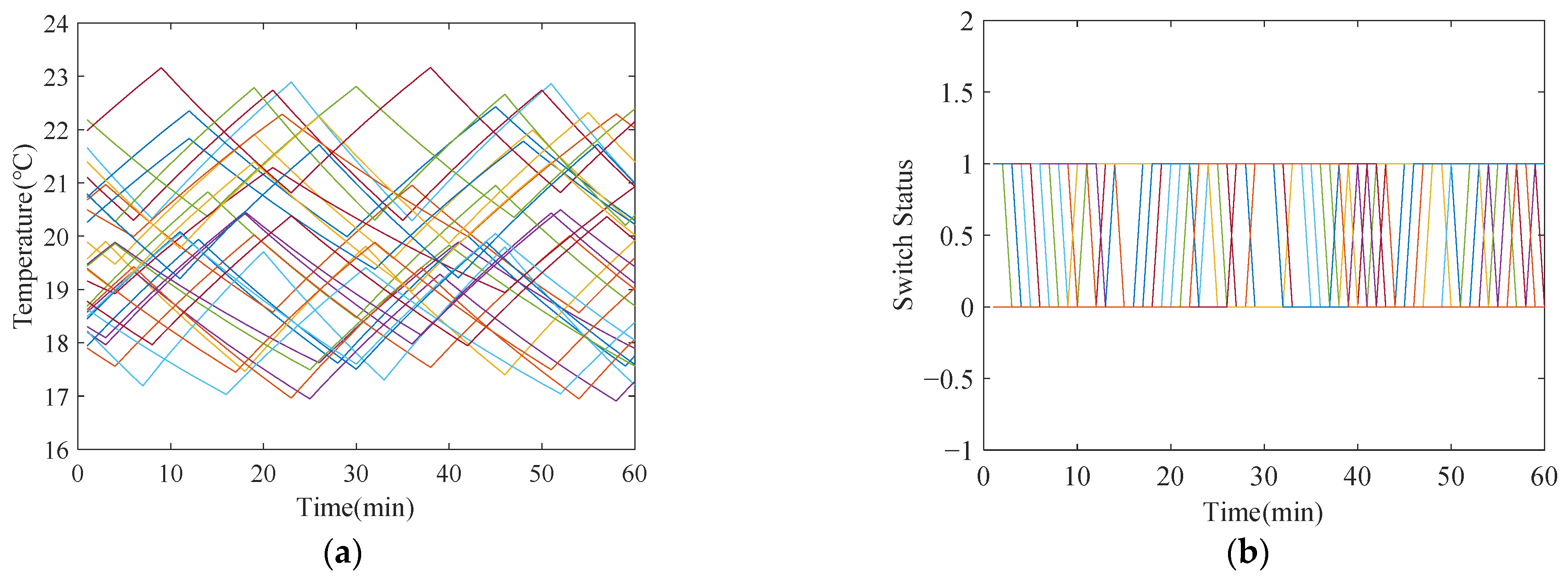
4.1. Air Conditioner Load Aggregation Model

Using the air conditioner load as an example, pertinent data indicate that starting from the summer of 2021, the summer air conditioner load in southern provinces like Zhejiang surpassed one-third of the peak power load, with some cities like Beijing even experiencing a 50% proportion of the summer air conditioner load. Therefore, selecting air conditioners to research in temperature control equipment has typical significance.

The heat transfer process in a room under the operation of air conditioner can be modeled using the lumped parameter method as an equivalent model:

$$\begin{array}{l}\{\begin{array}{l}{C}_{in}\frac{d{\theta }_{in}(t)}{dt}=P_{ac}(t)-\frac{{\theta }_{in}(t)-{\theta }_{wall}(t)}{R_{in}}\\ C_{wall}\frac{d{\theta }_{wall}(t)}{dt}=\frac{{\theta }_{in}(t)-{\theta }_{wall}(t)}{R_{in}}-\frac{{\theta }_{wall}(t)-{\theta }_{out}(t)}{R_{wall}}\end{array}\\ {\theta }_{in}(0)={\theta }_{in0},{\theta }_{wall}(0)={\theta }_{wall0}\end{array}$$

(18)

where $C_{in}$ and $C_{wall}$ are the equivalent heat capacity of the air in the room and the equivalent heat capacity of the room wall; ${\theta }_{in}$, ${\theta }_{wall}$, and ${\theta }_{out}$ are the indoor air temperature, room wall temperature, and outdoor temperature; $R_{in}$ and $R_{wall}$ are the equivalent thermal resistance of the air in the room and the equivalent thermal resistance of the room wall; and $P_{ac}(t)$ is the current operating power of the air conditioner, with the following status.

$$P_{ac}(t)=\{\begin{array}{l}S(t)\cdot P_{Ncool},{\theta }_{out}>{\theta }_{in}\\ S(t)\cdot P_{Nheat},{\theta }_{out}<{\theta }_{in}\\ 0,{\theta }_{out}={\theta }_{in}\end{array}$$

(19)

where $P_{Ncool}$ is the rated cooling power; $P_{Nheat}$ is the rated heating power; and $S(t)$ represents the current switch status of the air conditioner.

As an on–off air conditioner, it has the following switch states.

$$S(t)=\{\begin{array}{l}0,{\theta }_{in}\le T_{set}-T_{\lim it}\\ 1,{\theta }_{in}\ge T_{set}+T_{\lim it}\\ S(t-1),T_{set}-T_{\lim it}<{\theta }_{in}<T_{set}+T_{\lim it}\end{array}$$

(20)

where $T_{set}$ is the set temperature of the air conditioner; and $T_{\lim it}$ is the temperature control accuracy of the air conditioner.

Set the initial temperature of 30 rooms between 18 and 22 °C, and the following Figure 4 shows the load state changes using this model and control method.

In Figure 4, the curves of different colors in (a) represent the temperatures in different rooms, and it can be seen that the temperature difference in each room varies within one °C. The curves of different colors in (b) represent the switch states of the AC corresponding to different rooms. It can be seen that the switch states of the on–off air conditioners constantly switch between zero and one, controlling the room temperature within a certain range. To further describe this process, for example, in summer, if the set temperature of an air conditioner is 20 °C and the initial switch state is zero, allowing a temperature difference of 1 °C, it will remain in standby mode until the indoor temperature rises to 21 °C and the switch state of the air conditioner becomes one. It will remain in operation until the room temperature drops to 19 °C, and the air conditioner will enter standby mode again, with the temperature rising back to 21 °C, repeating this cycle.

By controlling the switch to vary with the difference between the outdoor temperature and the set temperature, the operating mechanism of inverter ACs in summer can be simulated, which can adapt to the situation where the load in the agent includes both an inverter AC and on–off AC.

$$S(t)=\{\begin{array}{l}0,{\theta }_{in}\le T_{set}-T_{\lim it}\\ 1,{\theta }_{in}\ge T_{set}+T_{\lim it}\\ \frac{\left|{\theta }_{in}-(T_{set}-T_{\lim it})\right|}{2\cdot T_{\lim it}},\\ T_{set}-T_{\lim it}<{\theta }_{in}<T_{set}+T_{\lim it}\end{array}$$

(21)

It should be noted that the above formula is only applicable to summer cooling; the operating mechanism of air conditioners in winter is slightly different from that in summer. So, this article selects the study of cooling in summer, which has certain representativeness.

Using the Monte Carlo method to evenly distribute the parameters of air conditioners and the initial temperature of the rooms within a certain range, combined with the variation curve of external temperature, the daily load curve of the air conditioner LA can be obtained.

The diagram of the difference between the on-off AC and inverter AC is shown in Figure 5 below, where both types of AC have a $T_{set}$ of 20 °C. The temperature of a certain city in summer was used as the outdoor temperature, and the change curve of this temperature during the day is shown by the green line in Figure 5b. The number of units aggregated for both types of air conditioner LAs is 600.

In Figure 5, the green curve in the figure represents the outdoor temperature. It can be seen that the blue curve representing the inverter AC has a relatively smooth power curve; when the outdoor temperature is high, the temperature difference between indoors and outdoors is large, and the power of the AC is high because the AC needs to maintain room temperature. The red curve representing the on-off AC shows a sawtooth shape because the higher the outdoor temperature, the higher the frequency of the AC being kept on; during that hot period, more air conditioning was maintained in the on state, which resulted in an increase in total power at a macro level.

When the air conditioner responds to demand, if peak shaving is required in summer, $T_{set}$ will increase, while $T_{set}$ will decrease when valley filling is required. The changes in $T_{set}$ during winter are opposite, and when $T_{set}$ undergoes corresponding changes, the aggregated power of the air conditioners will also change accordingly.

$$P_{DAC,i}(t)={\displaystyle \sum _{k\in i}{P}_{ac1,k}(t)}-{\displaystyle \sum _{k\in i}{P}_{ac2,k}(t)}$$

(22)

where $P_{ac1,k}(t)$ is the power of the k-th AC device belonging to the i-th agent before executing the demand response; and $P_{ac2,k}(t)$ represents the power of the k-th AC device of the i-th agent after the demand response.

4.2. Electric Vehicle Load Aggregation Model

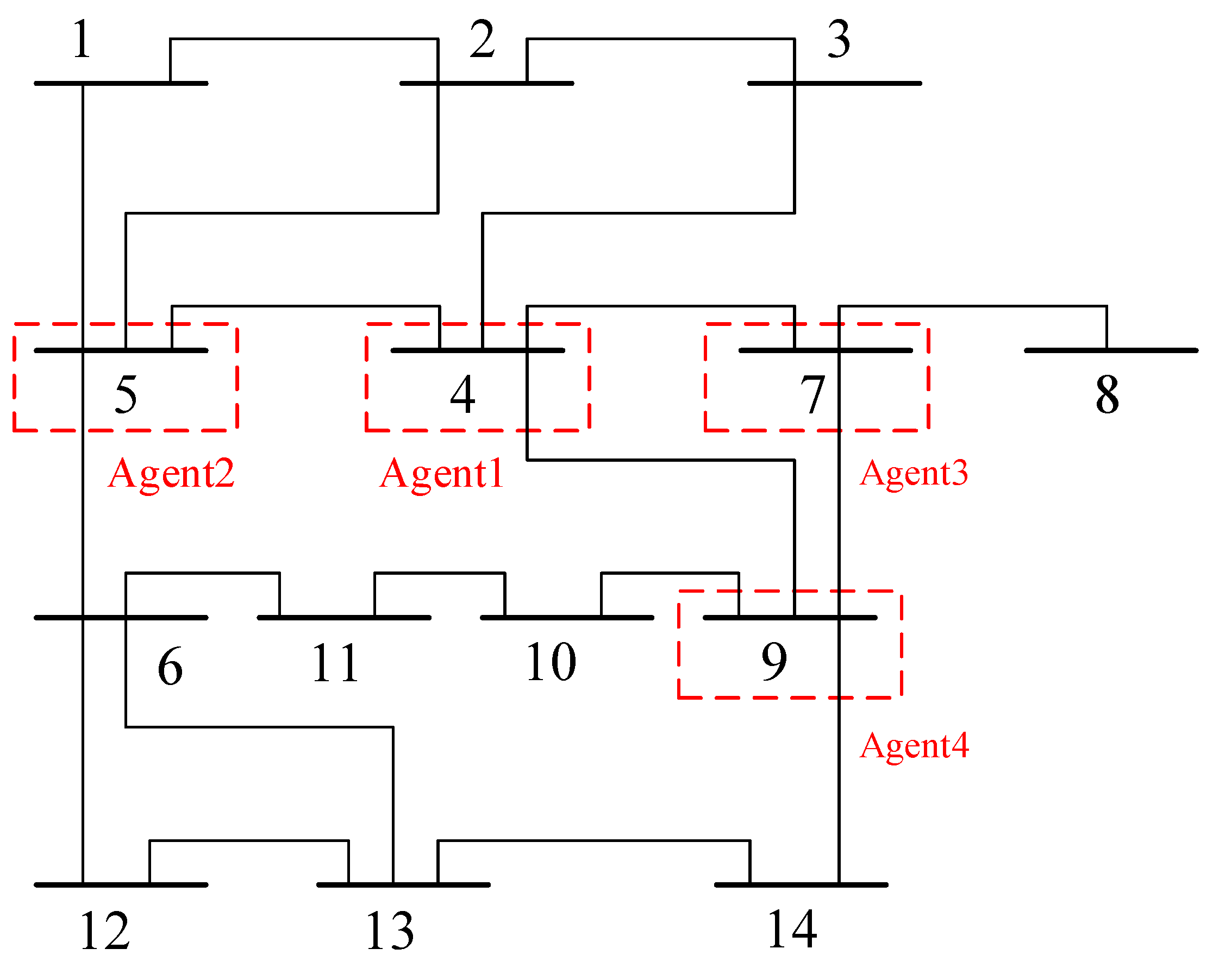
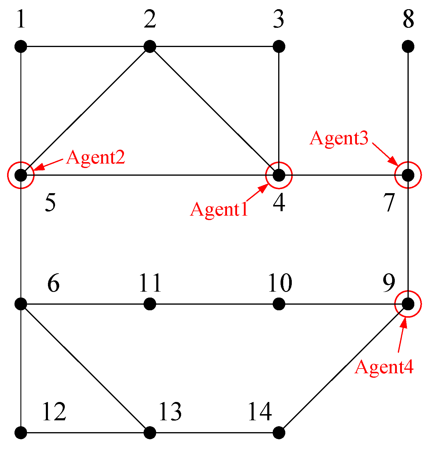
This article uses the Monte Carlo method and dynamic programming method to establish a model of electric vehicle load aggregation participating in demand response. It is known that with the support of a large amount of relevant data [29], probability density functions (PDFs) can be used to model the uncertainty of the daily travel distance of electric vehicles. The daily mileage $s$ of the vehicle follows the following logarithmic normal distribution:

$$g(s;\mu ,\sigma )=\frac{1}{s\sigma \sqrt{2\pi }}{e}^{-\frac{(\ln s-\mu )}{2{\sigma }^2}}$$

(23)

where $\mu$ is the mathematical expectation of the lognormal distribution; and $\sigma$ is the variance of the lognormal distribution.

The energy consumption of each electric vehicle can be seen as a direct proportion of the distance traveled, and according to the law of conservation of energy, the energy consumption of electric vehicles can also be expressed as the integral of charging power over time:

$$\begin{array}{l}{W}_{EV}^i=s^i\times w_{EV}^i={\displaystyle \int P_{EV}^i(t)dt},\\ t\in \{[t_{start1},t_{end1}]\cup [t_{start2},t_{end2}]\dots \}\end{array}$$

(24)

where $W_{EV}^i$ represents the energy consumption of each electric vehicle; $w_{EV}^i$ is the energy consumption per kilometer of the i-th electric vehicle; and $P_{EV}^i(t)$ is the charging power of each electric vehicle.

In the same electric vehicle load group, it can be seen that the $w_{EV}^i$ of each vehicle is the same, and there are generally two types of charging power, namely, fast charging and slow charging. The total energy or power of the electric vehicle load agent can be obtained by summing up the energy or power added to each vehicle.

Assuming that after the charging of an electric vehicle is completed, the battery level is sufficient to maintain during a trip without recharging; the start charging time of the electric vehicle is the return time of the electric vehicle, and the stop charging time is the departure time of the electric vehicle. Using the Monte Carlo method, the return time and departure time of the electric vehicle can be approximated as a segmented normal distribution, as shown below.

$$f(t_{start})\{\begin{array}{c}\frac{1}{{\sigma }_1\sqrt{2\pi }}{e}^{-\frac{{(t_{start}-{\mu }_1)}^2}{2{\sigma }_1^2}},({\mu }_1-12)<t_{start}\le 24\\ \frac{1}{{\sigma }_1\sqrt{2\pi }}{e}^{-\frac{{(t_{start}+24-{\mu }_1)}^2}{2{\sigma }_1^2}},0<t_{start}\le ({\mu }_1-12)\end{array}$$

(25)

$$f(t_{end})\{\begin{array}{c}\frac{1}{{\sigma }_2\sqrt{2\pi }}{e}^{-\frac{{(t_{end}-{\mu }_2)}^2}{2{\sigma }_2^2}},({\mu }_2+12)<t_{end}\le 24\\ \frac{1}{{\sigma }_2\sqrt{2\pi }}{e}^{-\frac{{(t_{end}+24-{\mu }_2)}^2}{2{\sigma }_2^2}},0<t_{end}\le ({\mu }_2+12)\end{array}$$

(26)

where ${\mu }_1$ and ${\sigma }_1$ are the expected and variance of the return time; ${\mu }_2$ and ${\sigma }_2$ are the expected and variance of the departure time.

The formula for calculating the total cost is as follows:

$$c(t)=\{\begin{array}{l}{c}_1,t\in [t_{valleystart},t_{valleyend}]\\ c_2,t\in [t_{peakstart},t_{peakend}]\end{array}$$

(27)

$$C_{sum}={\displaystyle \sum _{i=1}^n{\displaystyle \sum _{t\in T}{W}_{EV}^i(t)c(t)}},T=\{[t_1,t_2]\cup \left[t_3,t_4\right]\dots \}$$

(28)

where $c(t)$ is the electricity price when charging; $c_1$ is the valley electricity price; $c_2$ is the peak electricity price; $C_{sum}$ represents the total electricity bill; $W_{EV}^i(t)$ is the electricity usage during each charging period; and $T$ represents each charging period.

Develop a demand response strategy using charging path planning to obtain the total demand response capability and related parameters of the electric vehicle aggregation group. In general, users only choose fast or slow charging based on the distance they need to travel and the length of time they need to park. The start time of charging is the time of parking, and the end time of charging is the time to meet the travel needs of the day. By utilizing peak and valley electricity prices for vehicle charging planning, it is necessary to fully utilize the low-peak periods of electricity consumption when participating in demand response and re-plan the charging start and end times based on the corresponding parking periods of different users.

The path planning for the charging cost or charging power of electric vehicle load aggregation participating in demand response is shown in Figure 6 (this planning diagram is applicable to situations where the peak electricity price period starts and ends on the same day, and the valley electricity price period starts on the first day and ends on the next day).

Figure 6 shows that the load curves of electric vehicle LAs can be obtained, as well as the total load power at each time point and the reducible power during demand response.

$$P_{DEV,i}(t)={\displaystyle \sum _{k\in i}{P}_{ev1,k}(t)}-{\displaystyle \sum _{k\in i}{P}_{ev2,k}(t)}$$

(29)

where $P_{ev1,k}(t)$ is the power of the k-th electric vehicle charging station belonging to i-th agent before executing demand response; and $P_{ev2,k}(t)$ represents the power of the k-th electric vehicle charging station of i-th agent after demand response.

5. Example Analysis

5.1. Basic Parameters

This section takes the IEEE14 node distribution system as an example for simulation analysis. The specific structure of this system can be seen from Figure A1 and Figure A2 in Appendix B. Assuming that the connection relationship between distribution network nodes is unknown, reactive power is injected into the nodes, and Matpower is used to calculate the optimal power flow. The electrical distance is obtained as a parameter at the system level in the hierarchical optimization model. The simulation platform and environment for the thermal process and EV behaviors are all in Matlab 2021b.

The rated powers of the air conditioners are set to 0.1 times the rooms’ area, and the user’s room area follows a normal distribution with a mean of 80 and a variance of 10, ranging from 40 to 120 square meters. The outdoor temperature is simulated using a beta distribution based on the illumination intensity with a delay of 2 h. The initial temperature is set to 26 to 27 degrees Celsius; increase the set temperature by 2 degrees Celsius during demand response, and the temperature control accuracy is 1 degree Celsius. The expected departure time for electric vehicles is 7:00, the expected return time is 18:30, and the variance of both is 4 h. The electricity price during peak hours from 8:00 to 22:00 is 0.868 yuan/kWh, and the rest of the time is 0.588 yuan/kWh during peak hours. More parameters are provided in

Table A2. Variable reference value.

Variables	Value
$\epsilon$	0.002
$C_{in}$	6.61 × 103
$C_{wall}$	1.67 × 105
$R_{in}$	6.6 × 10−5
$R_{wall}$	$6$ 10−7
$P_{Ncool}$	8000
$P_{Nheat}$	8000
$T_{\lim it}$	1
$\mu$	30
$\sigma$	9
$w_{EV}^i$	0.2
${\mu }_1$	18.5
${\sigma }_1$	4
${\mu }_2$	7
${\sigma }_2$	4
$c_1$	0.588
$c_2$	0.868

of Appendix A.

The start time for demand response is 20 o’clock. The relevant load agents aggregated 500 air conditioners, 200 electric vehicles, 1000 air conditioners, and 500 electric vehicles, respectively. The initial state of the equipment was determined using the Monte Carlo method, and the relevant parameter settings of the agents are shown in

Table 1. Parameters for agents’ settings.

Parameters	Agent 1	Agent 2	Agent 3	Agent 4
Access node	4	5	7	9
Load aggregation type	AC	EV	AC	EV
Number of loads	1000	500	600	300
Coefficient ${\alpha }_i\times {10}^{-3}$	1.7	2.0	1.6	1.9
Coefficient ${\beta }_i\times {10}^{-3}$	297.4	254.1	257.1	281.0
Maximum DR power (kW)	1201	603	721	324

.

From the table, it can be seen that each load agent aggregates into power resources, with a maximum total power reduction of 2.85 MW.

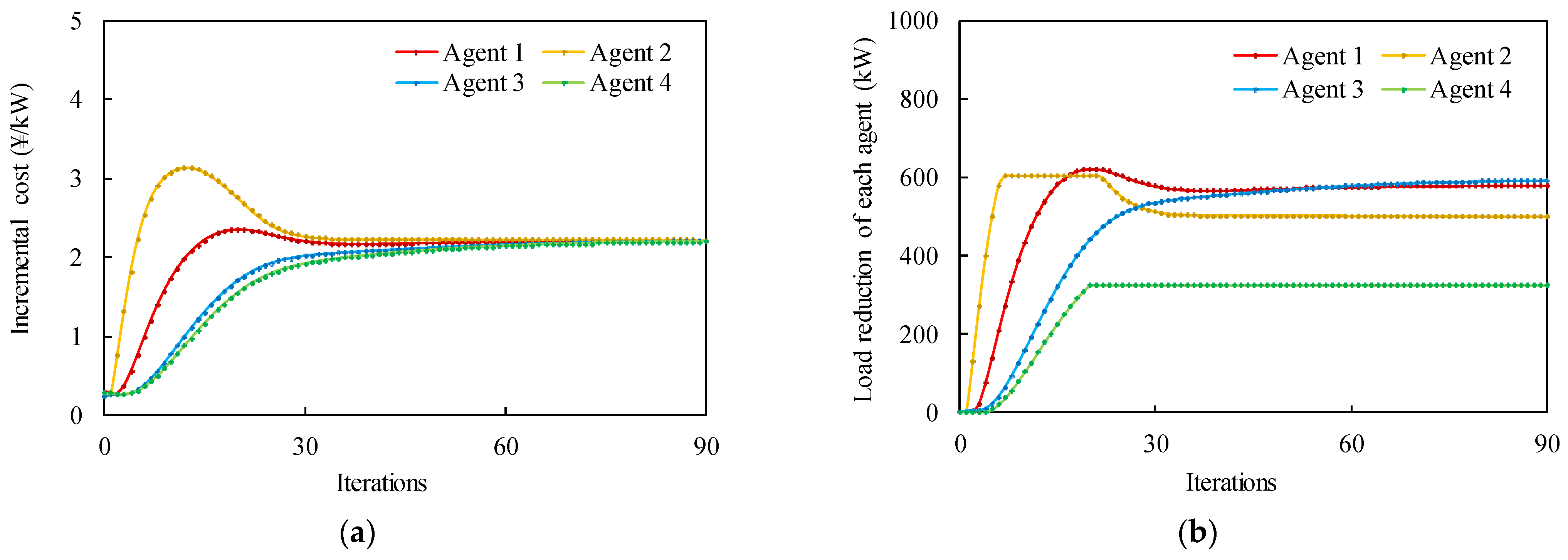
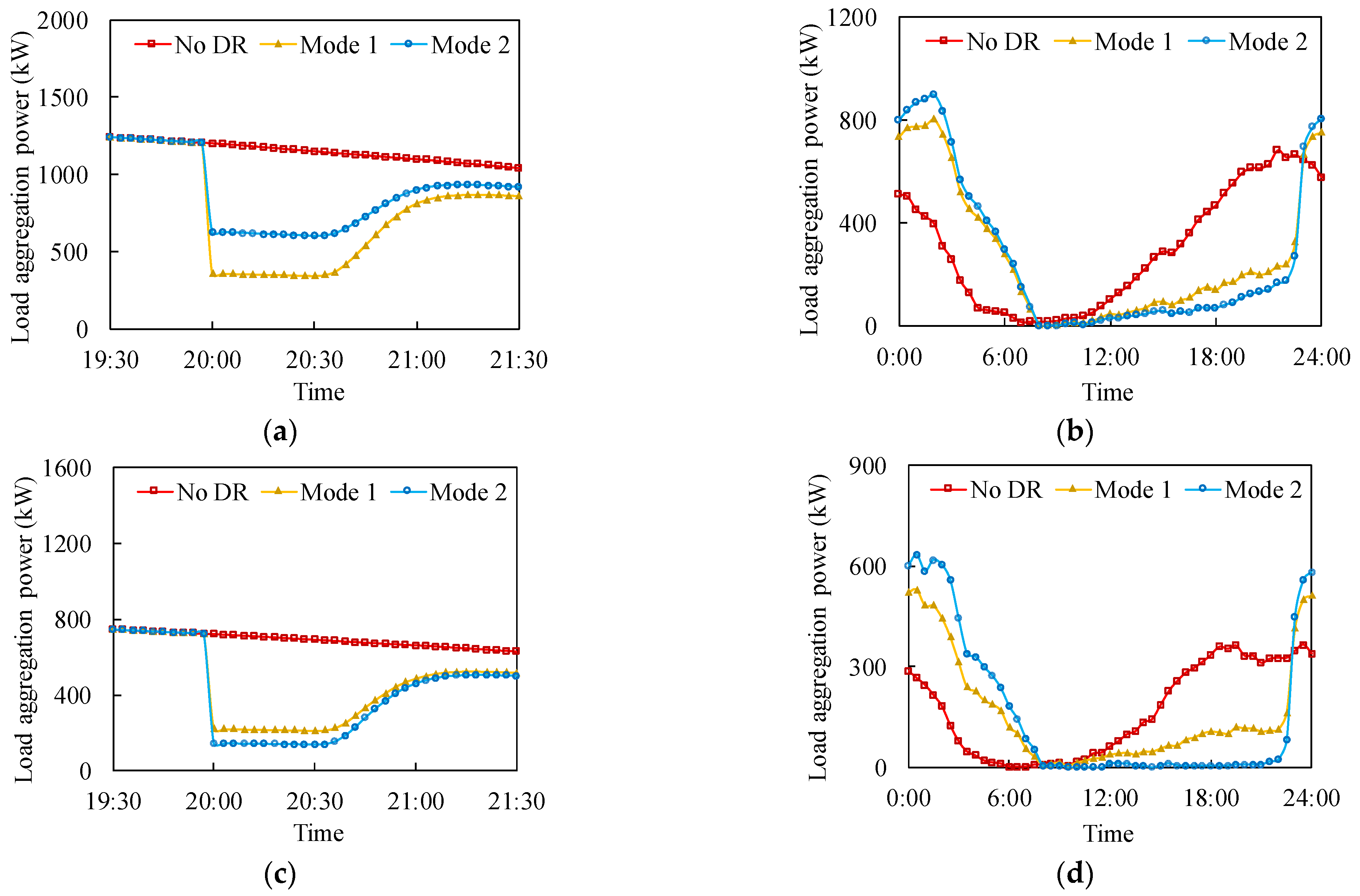
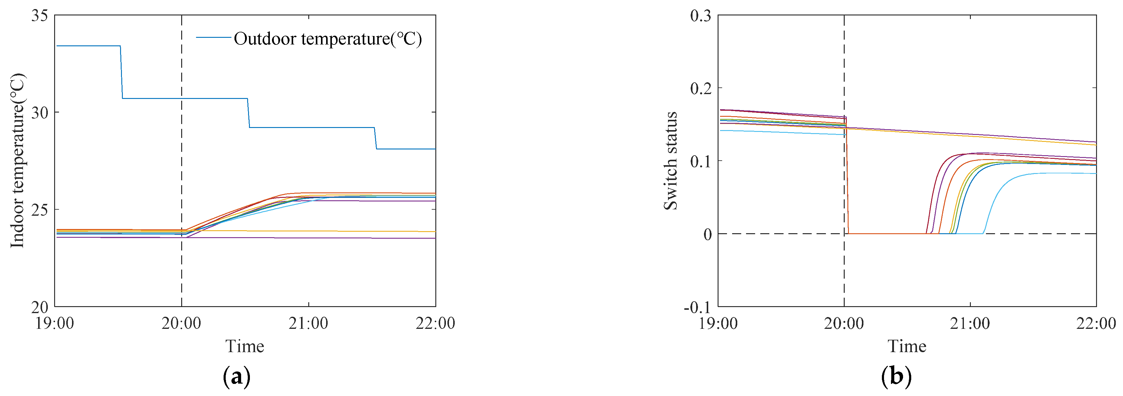
5.2. Evaluation of the Demand Response Ability of Agents

Based on the demand response strategy and parameter settings in this article, assuming the total load reduction of 2 MW, the optimization effect of the system layer in the hierarchical optimization model in Section 2.1 can be obtained, as shown in Figure 7.

In Figure 7, it can be seen that due to the limitations of their respective demand response capabilities, Agent 2 and Agent 4 reach the maximum load reduction first. As the solving process continues to iterate, Agent 3 gradually assumes more load reduction. The load reduction in Agent 1 and Agent 2 decreases in the later stage, which is basically similar to the trend of incremental cost, verifying the positive correlation between incremental cost and load reduction. For the total load reduction, it stabilizes after approximately 30 iterations, while each agent only reached a stable state after 40 iterations. This shows that in the practical application of the MAS, when the system assigns tasks to each agent, it may achieve the load reduction goal in advance.

To further verify its effectiveness, comparative experiments were conducted on other modes in this article.

In Mode 1, the system quickly allocated the target demand response amount based on the maximum response power ratio of each load agent. Therefore, the number of devices required for each agent to participate in demand response was calculated based on the proportion of the number of devices in an agent to the total number of devices, and the optimal incremental cost was not solved.

Mode 2 uses the method and strategy of demand response based on the MAS, reducing the costs using the hierarchical optimization model proposed earlier.

Combining the calculation results under this mode with the results in Figure 4, the relevant data can be obtained as shown in

Table 2. Comparison of demand response results.

Agent and Mode	Mode 1		Mode 2
	DR Load (kW)	Proportion of DR	DR Load (kW)	Proportion of DR
Agent 1	840	0.42	575.6	0.29
Agent 2	420	0.21	501.4	0.25
Agent 3	500	0.25	577.8	0.29
Agent 4	220	0.11	324	0.16

.

It can be seen that there are differences in the demand response value and demand response proportion of each load agent in the two modes. The task execution process of the agent layer, that is, the changes in the load curve of the aggregation model, are shown in Figure 8.

In Figure 8, it can be seen that different agents have different performance levels. The response speed of the AC load (Agent 1 and Agent 3) is fast, but the time scale is short. To maintain the user’s set temperature, the AC load needs to be increased after a period of time. The DR time maintained by the EV load (Agent 2 and Agent 4) is long, but the information of the agents needs to be investigated in advance. Each load has its advantages and disadvantages, so it is necessary to comprehensively utilize their strengths.

The temperature changes and information changes of AC equipment status in some typical rooms of AC load aggregation (controlled by Agent 1 and Agent 3) during the solution process are shown in the following Figure 9.

The curves of different colors represent the temperature of different rooms and the switch states of AC. In Figure 9, it can be seen that when the AC does not participate in DR, as the external temperature decreases, the indoor and outdoor temperature difference decreases. The power of the AC to maintain room temperature slowly decreases, and the switch state value slowly decreases; when the AC participates in DR, the switch quickly closes, but as the room temperature increases, the AC needs to turn on the switch to a certain extent to maintain the room temperature within the normal operating range.

During the process of DR using path planning, the daily electricity consumption and electricity bills of each user within the EV load aggregation can be obtained. The distribution histogram of the electricity bills paid by each user is shown in Figure 10.

The bar chart is set to transparent color for comparison of these three situations, and the overlapping parts represent the same number of users in the same electricity bill range. In Figure 10, it can be seen that the daily charging fees of most EVs were originally concentrated in the range of 7–11 yuan, but after DR, they became concentrated in the range of 7–8 yuan. This confirms that this optimization strategy can not only play a role in peak shaving or peak shifting in the power system, but also can reduce the cost of user charging, achieving a mutually beneficial situation between the power company and users.

Table 3. Comparison of electricity bills for EV agents in different modes.

EV Agent	No DR	Mode 1	Mode 2
Agent 2 (¥)	4544.64	3872.21	3738.66
Agent 4 (¥)	2787.88	2341.12	2129.23

shows the electricity bill statistics for Agent 2 and Agent 4 during this day.

The total power variation of the load connected to the system in both modes is shown in Figure 11.

In Figure 11, it can be seen that Mode 2 has a similar response speed compared to Mode 1, but Mode 1 cannot solve the optimal cost problem. Moreover, Mode 2 has better peak shaving and valley filling effects and is more economical. From the daily load curve, although the two models maintain the demand response target for a relatively short time, due to the complementary characteristics of multiple loads, they have a certain inertia. Compared to a single load, this aggregation method can reduce the ramp rate of power increase at the end of demand response, maintain the stability of the distribution network to a certain extent, and respond relatively quickly.

6. Conclusions

This article proposes a hierarchical optimization model using the MAS and related technologies; it facilitates the study of ways and strategies for multiple loads to participate in demand response. For the system layer in this model, a master–slave consistency algorithm is proposed to solve the allocation problem of each agent in the demand response task, and an arithmetic example is given. The results show that this method can adapt to most DR scenarios. A DR method for setting temperature and charging planning was proposed for the AC and EV loads in the model, and the Monte Carlo method was used to simulate the DR process of the load agent in the example. The results showed that the AC load was superior to the EV load in the short-term DR process, but EVs were superior to ACs in the long-term DR process. The results also showed that this method achieves complementary advantages among multiple loads, enabling them to achieve a balance between short-term and long-term DR processes.

In response to the lack of affinity between the MAS, distribution networks in the past, and the difficulty in scheduling various power loads, this article proposes a method of using electrical distance as the communication weight between agents, which facilitates communication between agents through distribution network nodes without the need to know the connection relationship between nodes. Therefore, the MAS can achieve fast computation. It also assigns demand response tasks from the system to agents, achieving load reduction in a black-box state. In addition, we also found in the experiment that the convergence speed of intelligent agents largely depends on hardware, and a large number of agents can indeed take up a longer solving time, but it is not enough to cause limitations in this MAS.

This article verifies the superiority of the MAS by comparing two modes of DR to handle the same load reduction task. Although the MAS proposed in this article requires distribution network-related data in advance, if the distribution network structure does not change, its relationship matrix can be reused multiple times. To further explore its ability, the impact of complex distribution networks and real-time changes in the distribution network structure on their computation speed should be studied in the future, and the types of loads should also be expanded. Grid operators can achieve the minimum total incentive provided to consumers while meeting the goal of electricity reduction, achieving the optimization of demand response costs.

There is still a lack of comparative methods and practical numerical validation in this study. Although incentive plans are proposed, there is still uncertainty about the level of user recognition and how to promote them, and the complexity of underlying load equipment interfaces exacerbates this uncertainty. In order to overcome the above limitations, in future research, we will strengthen technological research and development, carry out pilot applications, and open underlying device interfaces while ensuring security. We will be committed to continuously improving the intelligence level of the power grid and promoting high-intensity interactions between the power grid and users.

References

1. The People’s Political Consultative Conference Website (CPPCC). Local Development and Consumption Are the Key to Distributed “Wind and Solar Power”. Available online: http://www.rmzxb.com.cn/c/2021-07-13/2903585.shtml (accessed on 15 August 2023).
2. Tang, D.; Fang, Y.P.; Zio, E. Vulnerability analysis of demand-response with renewable energy integration in smart grids to cyber attacks and online detection methods. Reliab. Eng. Syst. Saf. 2023, 235, 109212. [Google Scholar] [CrossRef]
3. Bin, Y.; Zhenyu, C.; Yao, H.; Wenjun, R.; Hongquan, Z.; Zhiguo, G. Bi-Level Scheduling Model of Air Conditioning Load Aggregator Considering Users. In Proceedings of the 2020 5th Asia Conference on Power and Electrical Engineering (ACPEE): 1995–2001, Chengdu, China, 4–7 June 2020. [Google Scholar]
4. Wu, R.; Wang, D.; Xie, C.; Lai, C.S.; Huang, J.; Lai, L.L. Distributed control method for air conditioner load participation in distribution network voltage management. Autom. Electr. Power Syst. 2021, 45, 215–222. [Google Scholar]
5. Wang, L.; Han, L.; Tang, L.; Bai, Y.; Wang, X.; Shi, T. Incentive strategies for small and medium-sized customers to participate in demand response based on customer directrix load. Int. J. Electr. Power Energy Syst. 2024, 115, 109618. [Google Scholar] [CrossRef]
6. Wu, H.; Wang, J.; Lu, J.; Ding, M.; Wang, L.; Hu, B.; Sun, M.; Qi, X. Bilevel load-agent-based distributed coordination decision strategy for aggregators. Energy 2022, 240, 122505. [Google Scholar] [CrossRef]
7. Alipour, M.; Mohammadi-Ivatloo, B.; Moradi-Dalvand, M.; Zare, K. Stochastic scheduling of aggregators of plug-in electric vehicles for participation in energy and ancillary service. Energy 2017, 118, 1168–1179. [Google Scholar] [CrossRef]
8. Zhang, G.; Niu, Y.; Xie, T.; Zhang, K. Multi-level distributed demand response study for a multi-park integrated energy system. Energy Rep. 2023, 9, 2676–2689. [Google Scholar] [CrossRef]
9. Hu, D.; Liu, H.; Zhu, Y.; Sun, J.; Zhang, Z.; Yang, L.; Liu, Q.; Yang, B. Demand response-oriented virtual power plant evaluation based on AdaBoost and BP neural network. Energy Rep. 2023, 9, 922–931. [Google Scholar] [CrossRef]
10. Rocha, H.R.O.; Honorato, I.H.; Fiorotti, R.; Celeste, W.C.; Silvestre, L.J.; Silva, J.A.L. An Artificial Intelligence based scheduling algorithm for demand-side energy management in Smart Homes. Appl. Energy 2021, 282, 116145. [Google Scholar] [CrossRef]
11. Xu, Y.; Liu, W.; Gong, J. Stable Multi-Agent-Based Load Shedding Algorithm for Power Systems. IEEE Trans. Power Syst. 2011, 26, 2006–2014. [Google Scholar]
12. Hongfei, X.; Xin, C.; Hao, Q.; Yanyan, L. Secondary voltage regulation strategy applicable to master-slave control microgrids. Electr. Autom. 2020, 42, 20–22. [Google Scholar]
13. Shahbazi, H.; Karbalaei, F. Decentralized Voltage Control of Power Systems Using Multi-agent Systems. J. Mod. Power Syst. Clean Energy 2020, 8, 249–259. [Google Scholar] [CrossRef]
14. Mahela, O.P.; Khosravy, M.; Gupta, N.; Khan, B.; Alhelou, H.H.; Mahla, R.; Patel, N.; Siano, P. Comprehensive overview of multi-agent systems for controlling smart grids. CSEE J. Power Energy Syst. 2022, 8, 115–131. [Google Scholar]
15. Lee, J.W.; Kim, M.K. An Evolutionary Game Theory-Based Optimal Scheduling Strategy for Multiagent Distribution Network Operation Considering Voltage Management. IEEE Access 2022, 10, 50227–50241. [Google Scholar] [CrossRef]
16. Wang, Z.; Paranjape, R. Optimal Residential Demand Response for Multiple Heterogeneous Homes with Real-Time Price Prediction in a Multiagent Framework. IEEE Trans. Smart Grid 2017, 8, 1173–1184. [Google Scholar] [CrossRef]
17. Dai, M.; Li, H.; Wang, S. Development and implementation of multi-agent systems for demand response aggregators in an industrial context. Appl. Energy 2022, 314, 118841. [Google Scholar]
18. Mingkun, D.; Hangxin, L.; Shengwei, W. Multi-agent based distributed cooperative control of air-conditioning systems for building fast demand response. J. Build. Eng. 2023, 77, 107463. [Google Scholar]
19. Song, X.; Far, Z.; Menghu, F.; Zechen, W.; Li, M. Assessment Model of Demand Side Load Resources Promoting Non-Hydro Renewables Integration and Consumption. In Proceedings of the 2018 China International Conference on Electricity Distribution (CICED), Tianjin, China, 17 September 2018; pp. 2880–2883. [Google Scholar]
20. Wang, Z.; Paranjape, R.; Chen, Z.; Zeng, K. Layered stochastic approach for residential demand response based on real-time pric-ing and incentive mechanism. IET Gener. Transm. Distrib. 2020, 14, 423–431. [Google Scholar] [CrossRef]
21. Xiaoqing, H.; Liang, S.; Xiang, G.; Miao, Y.; Peng, C.; Hong, Z.; Zhe, W. Hierarchical Control Architecture and Decentralized Cooperative Control Strategy for Large Scale Air Conditioner Load Participating in Peak Load Regulation. In Proceedings of the 2018 China International Conference on Electricity Distribution (CICED), Tianjin, China, 17 September 2018; pp. 2925–2930. [Google Scholar]
22. Ye, Z.; Keyou, W.; Guojie, L.; Bei, H.; Zhaojie, L. Distributed layered control strategy for microgrids based on multi-agent consensus algorithm. Autom. Electr. Power Syst. 2017, 41, 143–149. [Google Scholar]
23. Gunduz, H.; Jayaweera, D. Modern power system reliability assessment with cyber-intrusion on heat pump systems. IET Smart Grid 2020, 3, 561–571. [Google Scholar] [CrossRef]
24. Prabawa, P.; Choi, D.H. Multi-Agent Framework for Service Restoration in Distribution Systems with Distributed Generators and Static/Mobile Energy Storage Systems. IEEE Access 2020, 8, 51736–51752. [Google Scholar] [CrossRef]
25. Ren, W.; Beard, R.W.; Atkins, E.M. Information consensus in multivehicle cooperative control. IEEE Control. Syst. Mag. 2007, 27, 71–82. [Google Scholar]
26. Zhang, W.; Xu, Y.; Liu, W.; Zang, C.; Yu, H. Distributed Online Optimal Energy Management for Smart Grids. IEEE Trans. Ind. Inform. 2015, 11, 717–727. [Google Scholar] [CrossRef]
27. Xiao, J.; Guo, X.; Feng, Y.; Bao, H.; Wu, N. Leader-Following Consensus of Stochastic Perturbed Multi-Agent Systems via Variable Impulsive Control and Comparison System Method. IEEE Access 2020, 8, 113183–113191. [Google Scholar] [CrossRef]
28. Beibei, W.; Xiaoqing, H.; Weiyang, G.; Yifeng, L.; Lin, K. Decentralized collaborative control strategy for large-scale air conditioner load regulation under hierarchical control architecture. Proc. CSEE 2019, 39, 3514–3527. [Google Scholar]
29. Dunnan, L.; Lingxiang, W.; Weiye, W.; Hua, L.; Wen, W.; Mingguang, L. Optimization scheduling of large-scale electric vehicle charging and swapping loads based on deep reinforcement learning. Autom. Electr. Power Syst. 2022, 46, 36–46. [Google Scholar]
Figure 1. A hierarchical optimization model for DR based on MAS and multiple load participation.
Sustainability 16 00902 g001
Figure 2. Schematic diagram of the steps for establishing an MAS with a simple topological structure based on graph theory.
Sustainability 16 00902 g002
Figure 3. Flowchart of using agents with LA functionality to participate in demand response through hierarchical optimization of DR model.
Sustainability 16 00902 g003
Figure 4. Temperature change and switch status of a single room for temperature-controlled LA: (a) schematic diagram of temperature changes for temperature-controlled LA; (b) schematic diagram of switch state changes for temperature-controlled LA.
Sustainability 16 00902 g004
Figure 5. Difference between on-off AC and inverter AC: (a) daily load curves of different air conditioner LAs; (b) the daily temperature changes of typical rooms controlled by two types of ACs and the outdoor daily temperature changes.
Sustainability 16 00902 g005
Figure 6. Dynamic programming diagram of EV participation in demand response based on peak valley price.
Sustainability 16 00902 g006
Figure 7. The process of solving demand response tasks at the system layer: (a) the solution process of incremental cost consistency solution; (b) distribution of load reduction for each agent.
Sustainability 16 00902 g007
Figure 8. The process of executing demand response tasks at the agent layer: (a) load curves of Agent 1 in different modes; (b) load curves of Agent 2 in different modes; (c) load curves of Agent 3 in different modes; (d) load curves of Agent 4 in different modes.
Sustainability 16 00902 g008
Figure 9. The process of control information change in AC load aggregation (Agent 1 and Agent 3): (a) indoor and outdoor temperature changes in typical rooms; (b) switching state changes of AC in typical rooms.
Sustainability 16 00902 g009
Figure 10. Histogram of the distribution of electricity bills for each user in EV load aggregation: (a) distribution of user charging costs for Agent 2; (b) distribution of user charging costs for Agent 4.
Sustainability 16 00902 g010
Figure 11. Changes in the daily load curve after multiple loads participate in demand response.
Sustainability 16 00902 g011