Abstract
Biomass is a viable and accessible source of energy that can help address the problem of energy shortages in rural and remote areas. Another important issue for societies today is the lack of clean water, especially in places with high populations and low rainfall. To address both of these concerns, a sustainable biomass-fueled power cycle integrated with a double-stage reverse osmosis water-desalination unit has been designed. The double-stage reverse osmosis system is provided by the 20% of generated power from the bottoming cycles and this allocation can be altered based on the needs for freshwater or power. This system is assessed from energy, exergy, thermoeconomic, and environmental perspectives, and two distinct multi-objective optimization scenarios are applied featuring various objective functions. The considered parameters for this assessment are gas turbine inlet temperature, compressor’s pressure ratio, and cold end temperature differences in heat exchangers 2 and 3. In the first optimization scenario, considering the pollution index, the total unit cost of exergy products, and exergy efficiency as objective functions, the optimal values are, respectively, identified as 0.7644 kg/kWh, 32.7 USD/GJ, and 44%. Conversely, in the second optimization scenario, featuring the emission index, total unit cost of exergy products, and output net power as objective functions, the optimal values are 0.7684 kg/kWh, 27.82 USD/GJ, and 2615.9 kW.
1. Introduction
There are now two main tendencies in terms of environmental and economic challenges. First, the Intergovernmental Panel on Climate Change (IPCC) states that significant adjustments to energy, land, urban infrastructure, and industrial systems are required to keep global heating to 1.5 °C with minimal overshoot [1,2]. Increasing public understanding of the factors that contribute to environmental deterioration is important for accelerating the global switch to low-carbon energy sources and achieving sustainable development [3].
The progressive expansion of domestic renewable energy sources (RESs), enhancement of energy efficiency, and reduction of import dependence on fossil fuels are some of the primary objectives of the EU energy strategy [4]. The optimal scheduling and integration of renewable energy sources and effective energy management face numerous obstacles. The integration and optimization of power generation are more challenging due to the unpredictable and uncertain character of RES, particularly wind and solar energy. Unlike solar and wind energy, biomass is a more dependable and controllable source of energy. Biomass is comprised of a wide range of materials such as agricultural waste, wood, municipal waste, algae, etc., and the abundance of these materials is an opportunity for a valuable energy source. The public’s increased acceptance of these technologies is a key component in using various RESs [5,6]. RESs increase the majority of the population’s access to energy, and reduce local and global pollutant emissions and increase the potential for local socio-economic development. Additionally, electricity produced from renewable resources significantly lowers greenhouse gas emissions and energy poverty [7,8,9]. Co-firing biomass and fossil wastes for energy production is still a viable option for the efficient use of industrial and agricultural waste. An important factor in the rise in global energy consumption is bioenergy. It is also the fourth-largest energy source in the world and likely to be an essential part of the renewable energy mix because of its green, low-carbon, and clean characteristics as well as its significant development potential [10,11,12].
The clean conversion of diverse types of solid biomass to gas by biomass gasification has the potential to become an important process. For a variety of uses, biomass has the potential to be converted into several types of biofuel and biochemical. Gasifiers are one of the more practical options for converting biomass into valuable energy commodities. There are various gasification agents like air, steam, and oxygen and differing temperatures and pressures have considerable effects on gasification processes. There are many different methods to do this. Updraft and downdraft are two of the configurations for fixed bed gasifiers, and the downdraft fluidized bed configuration generates syngas of higher heating value [13,14,15].
The lack of clean water is another significant problem nowadays, particularly in warmer and more crowded locations. Large-scale renewable energy-assisted desalination systems still have higher clean water-production costs than conventional fossil fuel-based systems. Energy and material resources are needed to create and operate water-purifying systems. The most effective desalination method, which may be combined with various RESs, is reverse osmosis (RO). Reverse osmosis technology is currently the best technology for treating sewage. A RO water filter system can be suitable for campus water, canteen water, drinking water, food-processing water, chemical-production water, experimental water, aquaculture water, industrial water, hotel water, bathing water, and other applications and industries. Advanced RO systems can be developed, and their designs can be made advantageous with accurate mathematical modeling of the RO system. Given that intermittent RESs can shorten the lifespan of RO membranes and other components, RES optimization is needed to meet the RO demand [16,17,18,19]. There are numerous power-generation cycles and configurations to provide the necessary power for RO units. One of the well known power cycles that can use biomass as fuel is the gas turbine (GT). GTs operate at high temperatures and, because of this, they are often combined with various power-production processes for heat recovery, such as closed Brayton cycles, Rankine cycles, and fuel cells [20,21].
Biomass is a viable and accessible energy source that can help address the problem of energy shortages in rural and remote areas. Another important issue for societies today is the lack of clean water, especially in places with high populations and low rainfall. The objective of this paper is to address both of these concerns by developing a sustainable biomass-fueled power cycle integrated with double-stage reverse osmosis water desalination.
2. Previous Works
Much research has been reported on the topics central to the present study, and key studies are described here.
2.1. Biomass-Based Power Generation
An effective technique that uses solar power as a heat carrier for biomass gasification is the combination of biomass and solar photothermal gasification. However, the effects of biomass ash can erode the heat carrier that delivers heat to the biomass feedstock, and the erosion problem worsens as the number of cycles rises. Li et al. [22] looked into the erosion and adhesion brought on by maize stalk ash (CSA) repeatedly sintering to heat carrier particles (Al2O3). The primary components in CSA that erode Al2O3 particles are K and Si, and the more sintering cycles there are, the deeper the erosion of these elements. Using thermodynamic laws, Yilmaz et al. [23] conducted a thorough thermodynamic assessment of an integrated plant using biomass in their work. Biogas generated from demolition wood biomass powers the multi-generation plant type. The plant’s primary components are a Rankine cycle, hydrogen production, compression of hydrogen, clean water-production system, biomass gasifier cycle, and gas turbine sub-plant. This facility produces clean water, power, hydrogen, and warmth. The findings show that the planned plant’s overall energy and energy efficiencies are 52.84% and 46.59%, respectively. Additionally, the biomass gasification unit has the greatest irreversibility rate of 12,685 kW, and the total irreversibility rate of the proposed cycle is 37,743 kW. To increase biomass utilization, Chen et al. [24] integrated supercritical CO2 power cycles, biomass gasification-based power generation, and coal-fired power production. The clean syngas produced by biomass gasification is utilized by a GT, and the hot exhaust that is produced is then used to heat the feedwater streams of the coal power plant and the CO2 stream of the sCO2 (supercritical carbon dioxide) cycle. The performance of the proposed scheme, based on a 2.22 kg/s biomass consumption rate and a 350 MW coal power plant, was investigated using thermodynamic and economic analyses. The findings showed that, when coal-generated net power remains constant, biomass-to-electricity achieves energy and exergy efficiencies of about 44% and 41%, respectively, at the design point. Roy et al. [25] proposed a novel externally fired GT, molten carbonate fuel cell, biomass gasifier, and water-heating facility that has been coupled to form a combined heat and power system, and performed thermodynamic and economic analyses. According to the optimization, the cogeneration system has the highest energy efficiency (41.2%) and the lowest levelized energy cost (0.044 USD/kWh).
2.2. Reverse Osmosis Desalination Unit
Using actual plant-operation data, Blanco-Marigorta et al. [26] performed an exergo-environmental analysis of a reverse osmosis desalination facility in the Canary Islands. The plant can produce 82,000 m3/day in theory. Depending on the energy recovery, the phases of reverse osmosis, the filtration technology, and the pressurization of the feed water, several combinations are conceivable. The high-pressure pump and the first-stage reverse osmosis membrane module are responsible for most of the exergy destruction. Abbasi et al. [27] examined the application of high-temperature thermal energy storage to create electricity, cooling, and fresh water, and assessed three different modes of a novel integrated system. The RO desalination unit produces fresh water while the absorption refrigeration cycle provides cooling. The proposed system’s energy efficiency is calculated to be 14.4% at most, while its energy efficiency is 40.5% with a total product cost rate of 30.5 USD/GJ. Nemati et al. [28] proposed a cogeneration system based on a series of two-stage organic Rankine cycles (STORC) using a zeotropic mixture as the working fluid integrated with a reverse osmosis desalination (RO) unit for waste heat recovery from a heavy-duty marine diesel engine. The proposed system is thermodynamically simulated and assessed thorough energy, exergy, and exergoeconomics analyses. The optimization results show that the values of the objective functions are increased by 37.0% and 59.1 USD/GJ, respectively, at the final Pareto frontier optimal design point. Abdolalipouradl et al. [29] presented two unique trigeneration systems based on single and double flash methods that produce power, hydrogen, and fresh water using geothermal energy, and carried out thermodynamic and exergoeconomic analyses. Both cycles employ reverse osmosis desalination, an organic Rankine cycle, and a proton-exchange membrane electrolyzer to produce hydrogen and fresh water. The results demonstrate that the double-flash trigeneration system (system 2) performs better from exergy and exergoeconomic viewpoints than the single flash-based one (system 1), leading to the achievement of the system’s optimum values for net power output, hydrogen production rate, desalinated water rate, and energy and exergy efficiencies. Pan et al. [30] investigated the performance of four different CO2 Brayton-based dual-loop cycles to harness waste heat from a dual combustion engine. They achieved a notable 7% enhancement in energy efficiency when integrating a carbon dioxide Brayton cycle with an organic Rankine cycle, compared to scenarios lacking waste heat recovery. In a separate study, Song et al. [31] proposed four configurations combining carbon dioxide Brayton and organic Rankine cycles utilizing geothermal water in Spain. These configurations exhibited a substantial increase in total electricity generation ranging from 22% to 45% when contrasted with the conventional supercritical carbon dioxide cycle. Furthermore, other researchers [32] examined the amalgamation of a supercritical carbon dioxide cycle and an organic Rankine cycle as a downstream cycle for fresh water production via reverse osmosis desalination, utilizing exhaust gases from a gas turbine. The utilization of supercritical carbon dioxide and organic Rankine cycles for waste heat recovery from the gas turbine resulted in a respective increase in overall efficiency by 10.9% and 2%. Additionally, Wang et al. [33] undertook an analysis and optimization of a trigeneration system comprised of an organic Rankine cycle, a supercritical carbon dioxide cycle, a gas turbine, and an absorption refrigeration system.
2.3. Merits of the Present Study
This proposed system in the present study is a cogeneration externally fired GT integrated with an intercooler sCO2 Brayton cycle and a regenerative organic Rankine cycle (ORC) fueled solely by biomass, coupled with a double-stage RO unit with a Pelton turbine (PT) for fresh water production. The use of biomass leads to significantly lower flue gas emissions because of its accessibility and ease of substitution compared to fossil fuels. This system shows generally how efficient and economically viable it is to use a biomass-based cycle for power and fresh water production. The considered biomass for this system is wood which is one of the most common and easy-to-access sources of biomass. This system is environment-benign due to its products and methods of power generation. Another positive aspect of this system is that it can be utilized in remote locations and places where clean water is not accessible. The benefit of using double-stage RO is that the higher amounts of water can be into drawn the unit and desalinated. Rejected brine from the RO unit has a substantial amount of pressure; to benefit from this, a PT is utilized to increase the outlet water of the system. A comprehensive study is conducted to evaluate the system’s viability from energy, exergy, exergoeconomic, and environmental points of view. To have a better perspective on the present system and to find the optimal value for key parameters of the system, two separate multi-objective optimization situations with various parameters are employed. The novelty of the investigation is in the new configuration of the system which is composed of three different types of power-generation cycles and an RO unit and its analysis. The study of this cycle is also comprehensive and covers all the aspect of a power and water dual generation system.
3. System Description and Assumptions
3.1. System Description
The system proposed here is comprised of four sub-cycles, three of which are power-generation layouts, while the last is a water desalination RO unit. The gas Brayton cycle is considered the main cycle and the other bottoming cycles function using its products. Biomass (wood) is turned into the syngas in the gasifier and is burned in the combustion chamber to run the system. A detailed description of biomass and gasifier parameters has been presented elsewhere [21]. After heating the compressed air in the heat exchanger (HE) no. 1, product gases also heat the CO2 using HE2 in the intercooling Brayton cycle as well as R123 with HE3 in the ORC for high heat recovery. A portion of the generated power from the bottoming cycles is allocated to the multiple pumps in the double-stage RO unit. Additionally, generated power in the Pelton turbine is also utilized in the RO unit. Initially, water is drawn into the unit by the feed pump (FPu) and its pressure is raised to the required level (which is 6.23 MPa in this case for the reactions that take place) by the second stage of compression in the high-pressure pump (HPPu). At this step, high-pressure water goes through multiple layers of desalination filters at stage 1, and the rejected brine is then pressurized to the required pressure by the boost pump (BPu). After the second stage of desalination, the brine is expanded to the environmental pressure in the Pelton turbine which has the advantages of simple construction, easy maintenance, and high overall efficiency. Figure 1 illustrates the overall proposed system.
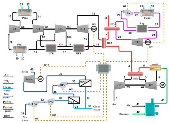
Figure 1.
Schematic of the proposed system.
3.2. Assumptions and Key Parameters
Several assumptions are considered for the system’s thermodynamic simulation:
- The system performs at steady state.
- Ambient temperature and pressure are considered to be 298 K and 101.3 kPa, respectively.
- Heat losses at heat exchangers, condensers, and recuperators can be neglected.
- R123 leaves the condenser as a saturated liquid.
Table 1 lists data for the important and key parameters of the system.

Table 1.
Key system parameters and their values [29,34].
4. System Modeling
4.1. Thermodynamic Modeling and Analysis
In this section, the system with its components is thermodynamically assessed and characterized, in part for the purpose of conducting an exergoeconomic analysis subsequently. When modeling the existing system, we consider the potential and kinetic energy of each stream and the pressure drop across the entire system to be insignificant and the system to operate under steady-state conditions. The assessment utilizes rate balances for mass, energy, and exergy, which follow:
In the current work, a downdraft gasifier which has four zones—drying, pyrolysis, reduction, and combustion—is considered.
4.1.1. Gasifier
According to the equilibrium model, all gasifier reactions should be in thermodynamic equilibrium. Before exiting the gasifier, the pyrolysis products are supposed to burn and reach equilibrium in the reduction zone. The reactions that take place during gasification are:
Based on Zainal et al. [35], the overall gasification reaction for the downdraft gasifiers is written as:
In Equation (8), w and m represent the values of water and oxygen per kmol of biomass, respectively. The biomass is mainly composed of carbon, hydrogen, and oxygen, while the municipal waste also contains a small fraction of nitrogen. Zainal et al. [35] assume that municipal waste has a composition of CH1.502O0.5189N0.02162 and a higher heating value (HHV) of 433,034 kJ/kmol. Soltani et al. [34] consider a complete combustion reaction in the CC by the mixture of syngas and air from GT1, which can be expressed as:
Soltani et al. [34] define the equilibrium constant for the methane formation as:
and the shift reaction as (Soltani et al. [34]):
By using the syngas coefficient values, we can calculate the equilibrium constant values for the methane generation and water–gas shift reactions. Soltani et al. [34] give the equilibrium constants for these reactions via Equations (10) and (11), respectively:
and
Soltani et al. [34] and Zainal et al. [35] provide other relevant equations such as equilibrium constants for simulating the gasification process.
4.1.2. Reverse Osmosis Unit
The RO module transforms seawater into fresh water by elevating its pressure in both the FPu and High-Pressure Pump (HPPu). Additionally, a portion of the required energy for the BPu is supplied by a Pelton turbine. This energy is utilized to boost the pressure of the discharged saline water from RO-1, enabling a repeat of the desalination process with RO-2. The following three equations are employed to establish the salinity levels of the brine and fresh water:
Here, y and ys are the clean water mass fraction and salt water mass fraction, respectively.
4.1.3. ORC Cycle
The ORC constitutes a pivotal element in the system modeling, serving as an efficient thermodynamic process for power generation. In the ORC, a working fluid (R123) with a lower boiling point than that of water is employed to transfer heat from a heat reservoir to the working fluid which has the advantage of waste heat recovery at heavy load. This heat causes the fluid to vaporize, driving a turbine and subsequently generating power. The mathematical representation of the Organic Rankine Cycle (ORC) involves several equations that capture the energy balance, heat transfer processes, and overall performance. Below are the fundamental equations describing the key components of the ORC cycle:
Energy rate balance for the condenser:
Energy rate balance for the turbine:
Net work output rate:
where
The efficiency of the ORC can be written as:
4.1.4. sCO2 Cycle
The expansion and compression processes in the sCO2 cycle are important components influencing the overall efficiency. CO2 is chemically inert and nontoxic and is non-flammable. Detailed modeling of the turbine and compressor involves accounting for isentropic efficiencies, pressure ratios, and temperature changes. The turbine, where the sCO2 expands, and the compressor, where it is compressed, play significant roles in determining the net work output of the cycle. Relevant energy rate balances for these devices, specifically C1, C2, REC, and ST1, respectively, follow:
The effectiveness of heat exchange significantly impacts the overall cycle efficiency, making it necessary to analyze the performances of recuperators, precoolers, and reheaters. Energy balances for devices HRT, LTR, Pre1, and Pre2 are as follows:
Equations for the energy analysis of the system are listed in Table 2.

Table 2.
Governing energy equations of the system.
4.1.5. Exergy Equations
Exergy analysis merges the principles of the second law of thermodynamics with equations governing mass and energy balances. A general exergy rate balance follows:
Here, represents the rate of exergy associated flows (inflow or outflow) for the component, and denotes the exergy destruction rate in device i. This equation underscores the significance of the dead state temperature (To) and the boundary temperature (T) in determining the rates of exergy destruction, or available energy dissipation, within the device. While certain constituents, such as air, exhibit zero or little chemical exergy due to their compositions relative to the reference environment, RO cycles, which involve variable compositions, necessitate specific mathematical expressions (refer to Table 3). For the system, the ratio of individual exergy destruction of component k to the overall exergy destruction can be expressed as

Table 3.
Governing exergy equations of the system.
4.1.6. Exergoeconomic Equations
This section delves into the amalgamation of exergetic and economic principles for system assessment, which gives rise to exergoeconomic concepts with the goal of minimizing both total cost and exergy destruction [36]. First, the evaluation includes presenting the cost equilibrium for the kth component using Equation (32), which asserts that the cost rate of input exergy combined with the investment cost rate of a component equals the cost rate of output exergy. Employing the average cost per unit of exergy (c), which is needed to analyze the system’s products, the method determines each stream’s cost rate (). That is,
where
Here, is the sum of capital investments and maintenance cost rates as follows [36]:
where CRF denotes the capital recovery factor, ∅r denotes the operation and maintenance factor, and Zk corresponds to the purchased equipment cost associated with the kth component. The CRF is dependent on the anticipated life cycle (n) and the interest rate (i), as follows [36]:
Note that the costs of the components need to be standardized, adjusting them from the reference year to the analysis year (2023 here) as follows [36]:
Moreover, the exergoeconomic factor () is applied to assess the components. The exergoeconomic factor indicates the proportional importance of non-exergy-related costs () and costs linked to exergy destruction and exergy loss () for each individual component [36]:
The relative cost difference (rk), which represents the deviation of product cost and fuel cost relative to fuel cost, can be written as
Details regarding the necessary cost balance and auxiliary equations for all components of the system are given in Table 4 and Table 5 [36].

Table 4.
Exergoeconomic equations for components of the system.

Table 5.
Expressions for purchase costs of devices used in the system [37].
5. Results and Discussion
5.1. Parametric Assessment
In this section, a comprehensive parametric investigation is undertaken to discern the influences of key parameters, including RPsCO2, CETDHE2, CETDHE3, and T3. The purpose of this investigation is to elucidate the contributions of these parameters to the thermodynamic behavior of the system.
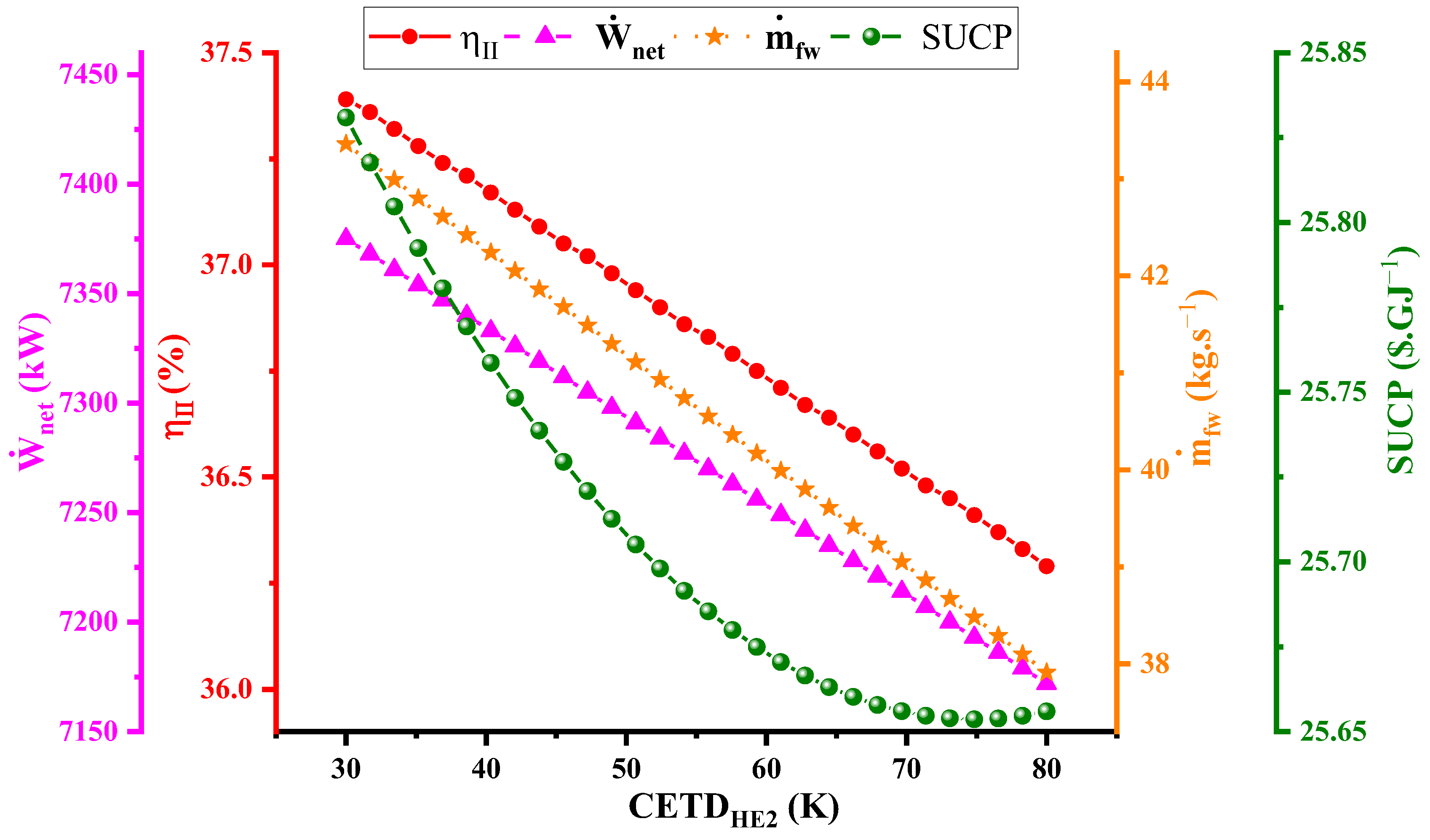
Figure 2 shows the complex interaction between RPGTC and four key variables: , , , and SUCP. Notably, the green curve illustrating the connection between RPGTC and SUCP demonstrates a gradual upward pattern from its starting point; this patter occurs because, as the value of RPGTC increases, the turbine and compressor have a more complex structure, which increases the price. Interestingly, the lowest point of SUCP is seen at RPGTC = 8, while the highest is reached at RPGTC = 16. Simultaneously, another curve is used to show how behaves with changes in RPGTC. At the beginning of the figure, there is a decrease until it reaches the lowest value, approximately at RPGTC = 11.5. Following this, there is a subsequent increase that continues until the end. The reason for this behavior is that the gas turbine generates the largest portion of the produced net power and is the most efficient cycle. Therefore, when the efficiency is at its maximum, the gas turbine cycle absorbs most of the heat from the exhaust gas, and the power production in bottoming cycles drops. As mentioned, the RO unit only uses a portion of the bottoming cycles’ produced power so the clean water production decreases as well. The changes in RPGTC concerning and are opposite to the RPGTC relationship. Initially, there is a positive incline, reaching the highest values of and η at RPGTC = 11.5. After this peak, both variables start to decrease. The turbine’s net work output and increase with rising RPGTC, and the turbine’s net work exceeds the work consumed by the compressor. However, after the RPGTC value reaches 11.5, the additional work produced in the turbine cannot exceed the additional work consumed by the compressor, resulting in a downward trend in the graph.
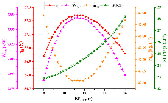
Figure 2.
Relationship between RPGTC and parameters , , , and SUCP.
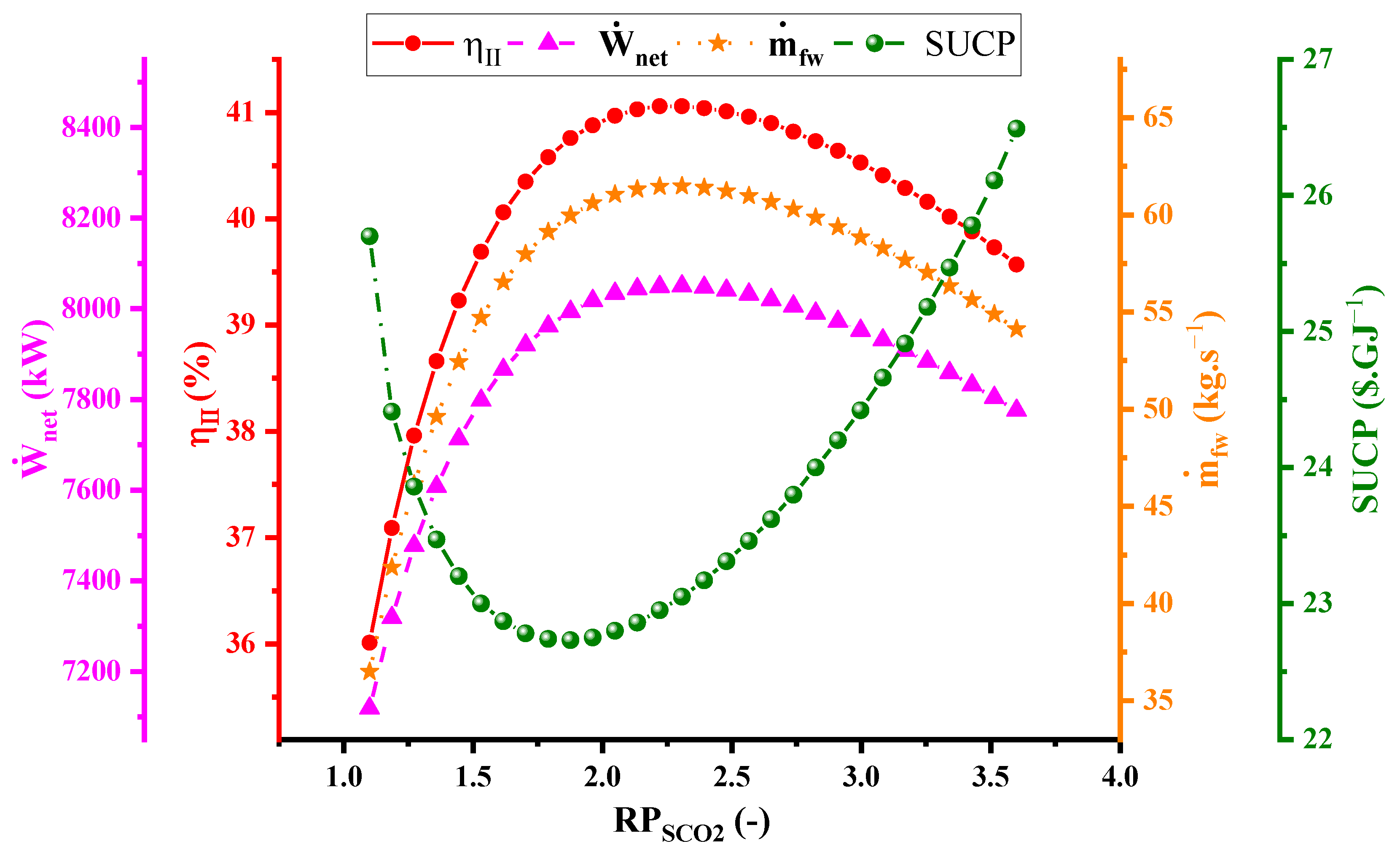
Figure 3 illustrates of the relationships between RPsCO2 and the parameters , , , and SUCP. It is evident that three of these curves, RPsCO2, RPsCO2–, and RPsCO2–, exhibit a closely aligned behavior characterized by an ascent leading to a peak, where all three variables (, , ) attain their maximum values at RPSCO2 = 2.23, followed by a subsequent descent. After the RPsCO2 value reaches its maximum, the turbine continues to produce power, and its value is greater than the consumption in the compressor. However, after passing the maximum value, the compressor’s consumption will exceed the turbine’s production due to the fact that some of the production power is consumed in the reverse osmosis unit. RPsCO2– shows a behavior similar to RPsCO2–. In contrast, the fourth curve (RPsCO2–SUCP) portrays a distinct trend whereby the initial increase in RPsCO2 results in a decrease in SUCP. However, after reaching the lowest point of SUCP at RPsCO2 = 1.88, the trend reverses, leading to a rise in SUCP with further RPsCO2 increases.
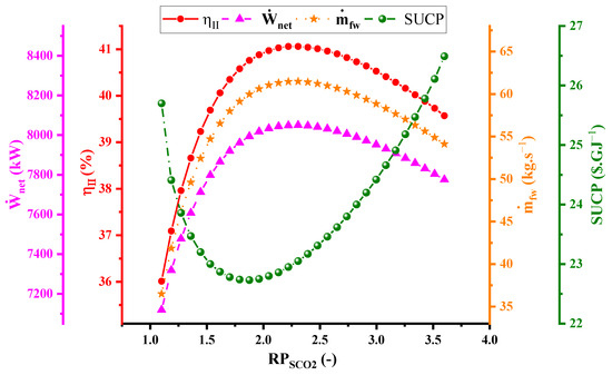
Figure 3.
Relationship between RPSCO2 and the parameters , , , and SUCP.
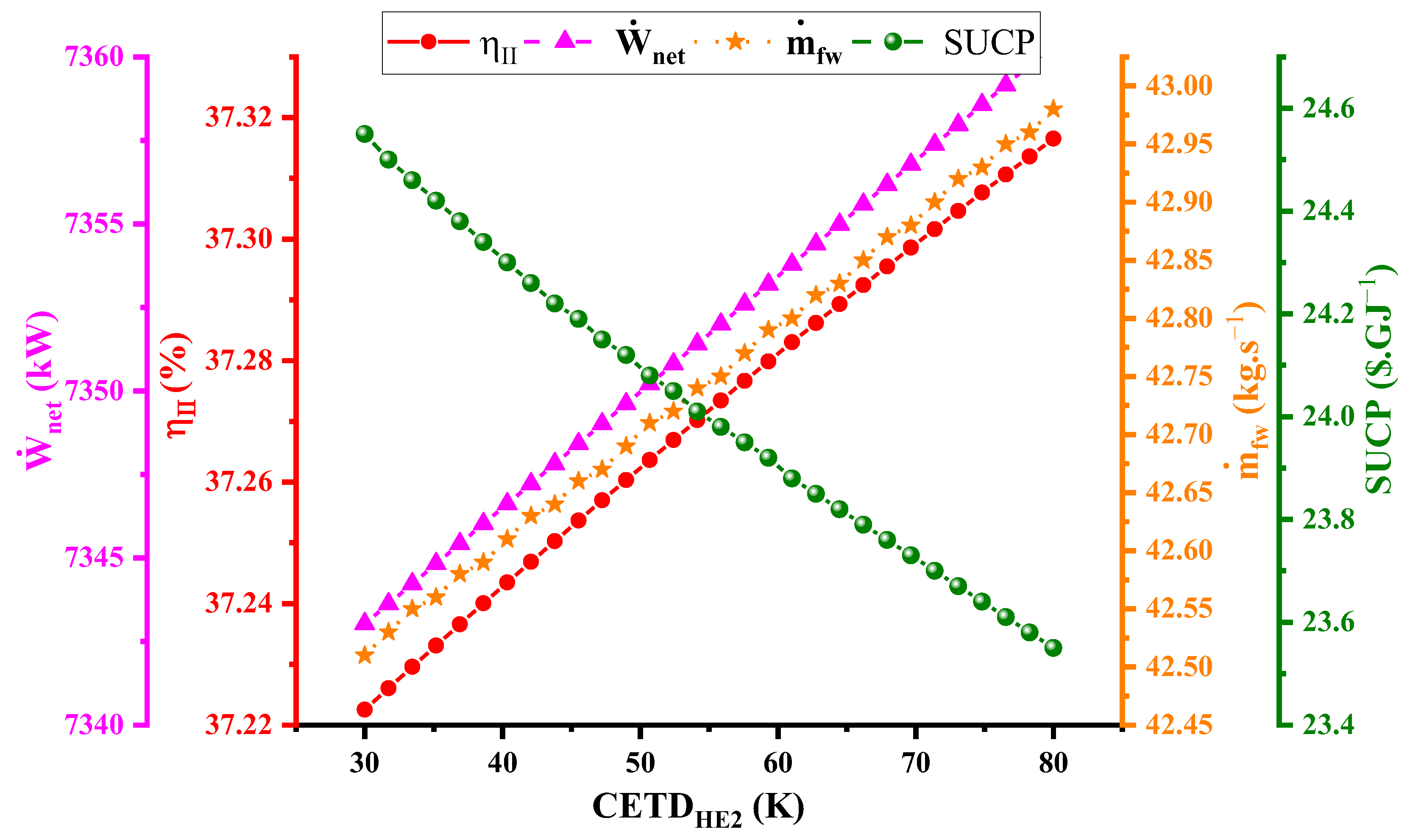
Figure 4 presents data pertaining to the correlation between CETDHE2 and four other variables: Wnet, η, mfw, and SUCP. These variables collectively exhibit a linear variation. Specifically, those associated with , , , and SUCP display positive inclines, with their lowest point observed at CETDHE2 = 30, and the highest point at CETDHE2 = 81. Conversely, the correlation involving SUCP exhibits a negative incline, with its minimum occurring at CETDHE2 = 81 and its maximum at CETDHE2 = 30. As the value of CETDHE2 decreases, the heat transfer increases, leading to an increase in efficiency. With a rise in CETDHE2, the heat exchanger’s structural complexity which is based on its effectiveness in heat transfer decreases, and the device’s cost is reduced.

Figure 4.
Relationship between CETDHE2 and four variables: Wnet, η, mfw, and SUCP.
Figure 5 comprises four graphs, three of which elucidate the interdependencies among , , , and CETDHE3. These graphs collectively manifest a linear pattern, characterized by near-identical slopes. For a cycle with constant fuel injection, variations of the net produced power and efficiency of the system are aligned. As mentioned earlier, the production rate of clean water is proportional to the generated power. Across all three graphs, the apex is observed at CETDHE3 = 32, while the minimum resides at CETDHE3 = 80. Contrastingly, Figure 6, which corresponds to the variable SUCP, diverges from the preceding triad in its behavior. This curve follows a parabolic trend, and its minimum point occurs at CETDHE3 = 58. By reducing the value of CETDHE3, , , and the amount of fresh water produced all decrease. Considering that, with an increase in CETDHE3, the device is less complicated and the price also decreases. However, after it reaches the minimum value, the efficiency becomes very low, making it incompatible with cheap devices.
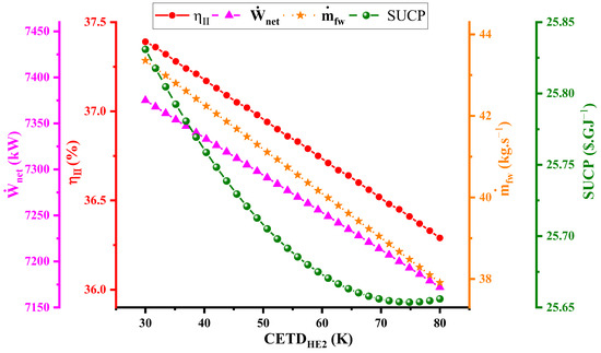
Figure 5.
Relationship between CETDHE3 and , , and .
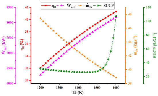
Figure 6.
Relationship between T3 and SUCP, , , and .
Figure 6 shows the correlations among four variables, SUCP, , , and, , in relation to T3 (temperature), and exhibit a diverse array of behaviors. The graph illustrating the T3 relationship displays a descending trend, progressively declining as T3 increases (based on the energy equation for HE1). Increasing the production power of the turbine decreases the thermal energy in the exhaust gases, resulting in less energy to transfer to other cycles. Considering that the electricity required by the reverse osmosis unit is supplied from the bottom cycles (sCO2 and ORC), the rate of fresh water production decreases because the electricity production decreases. Conversely, the T3 and T3 graphs show an ascending pattern, with values steadily rising as temperature escalates. Finally, the T3–SUCP plot demonstrates a relatively constant state initially, but upon reaching a temperature of 1500 K, it undergoes an abrupt vertical ascent. This sudden increase is a manifestation of the formula used to calculate the turbine’s price; as the turbine works at a higher temperature, it is more complicated and has a higher price.
5.2. Optimization
This section focuses on the merging of machine learning principles into the domain of optimization, enriching the pursuit of optimal solutions. Within this framework, machine learning techniques analyze data to discern patterns and inform decisions. The optimization process unfolds through various stages: data collection, preprocessing, feature engineering, model training, and the application of optimization methods like the “gray wolf algorithm,” alongside performance evaluation and iterative refinement. This integration facilitates data-driven decision-making processes.
In the realm of multi-objective optimization, the primary goal is to ascertain the most favorable operational configuration for a system by considering different influencing factors. Specifically, the aim is to simultaneously maximize the system’s net output power and exergy efficiency while minimizing the cost of exergy per product unit and the carbon dioxide emission index. For this, a thermodynamic model of the system is crafted using EES software (V10.561), addressing equations pertaining to energy, exergy, environmental considerations, and exergy economics.
The optimization starts with the introduction of 300 random points into an artificial neural network, encompassing crucial decision-making variables as input and important performance indicators (objective functions) as output. The neural network, structured with ten layers in a feedforward configuration, effectively models the input data and predicts related output values. This training process establishes a mathematical relationship between inputs and outputs. Post-training, the resulting network, serving as a fitness function, collaborates with the gray wolf algorithm to initiate the optimization process.
The gray wolf algorithm iteratively improves and optimizes the trained model using its unique approach. The optimization endeavor employs five inputs as decision variables, detailed in Table 6. MATLAB software (R2022a) serves as the computational tool for machine learning and multi-objective optimization employing the gray wolf algorithm in this study. Fine-tuning efforts are undertaken to achieve optimal values. Two distinct optimization scenarios are considered: the first scenario comprises the pollution index, total exergy unit cost of products, and exergy efficiency as objective functions, while the second scenario includes the pollution index, total exergy unit cost of products, and net output power as objective functions [38].

Table 6.
Lower and upper bounds of decision variables used in the optimization.
Results of Multi-Objective Optimization Using the Gray Wolf Algorithm
Utilizing the grey wolf algorithm, two distinct multi-objective optimization analyses were conducted, each employing a variety of objective functions such as environmental index ζ (kg/kWh), net output power (kW), exergy efficiency, and cost of product cp (USD/GJ). The outcomes of these optimizations for the first and second model optimization are depicted in Figure 7a,b.
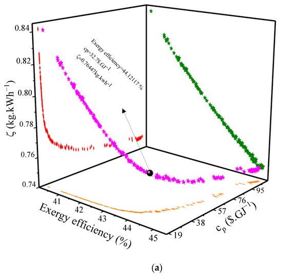
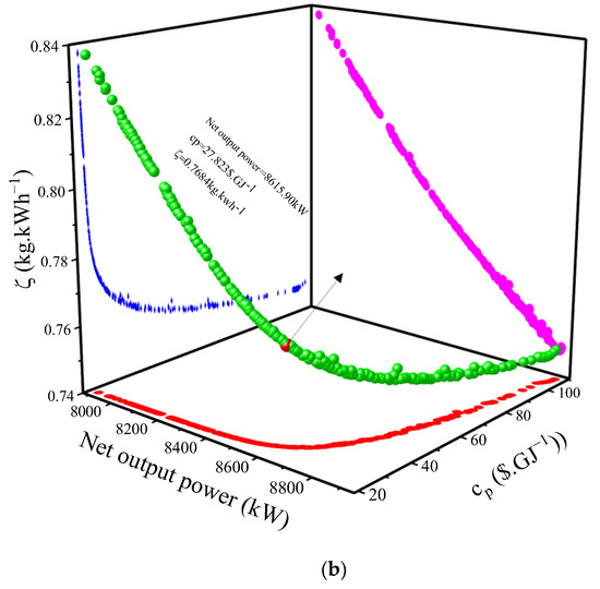
Figure 7.
(a) Pareto frontier for the first model multi-objective optimization. (b) Pareto frontier for the second model multi-objective optimization. The application of genetic algorithms to multi-objective optimization produced Pareto frontiers for both scenarios, as illustrated in (a,b). The proposed optimal values, taking into account three variables—ζ, cp, and exergy efficiency—are 0.7644 kg/kWh, 32.7 USD/GJ, and 44.12%, respectively. Moving to the second scenario, considering three variables—ζ, cp, and net output power—the values stand at 0.7684 kg/kWh, 27.823 USD/GJ, and 2615.90 kW, respectively.
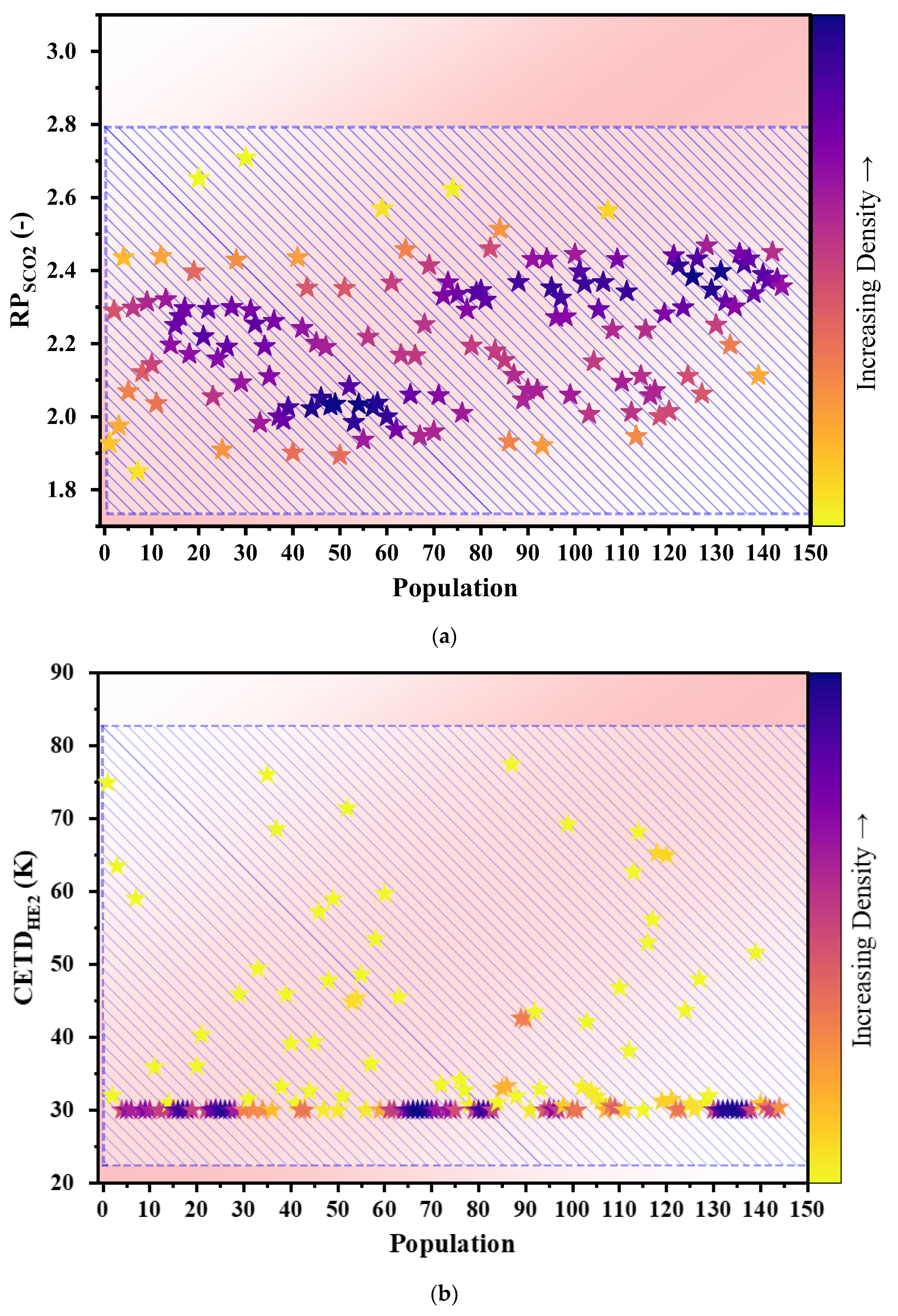
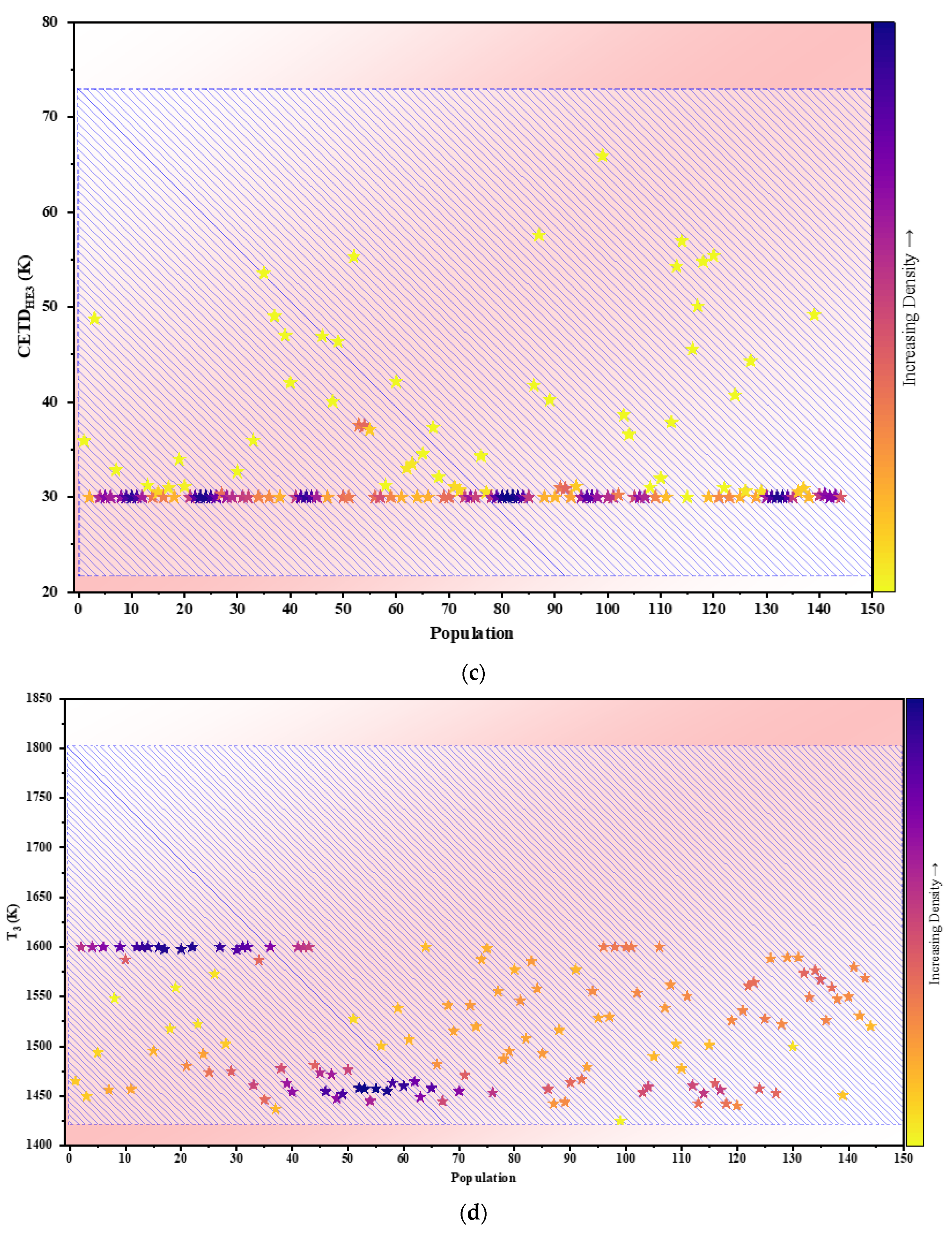
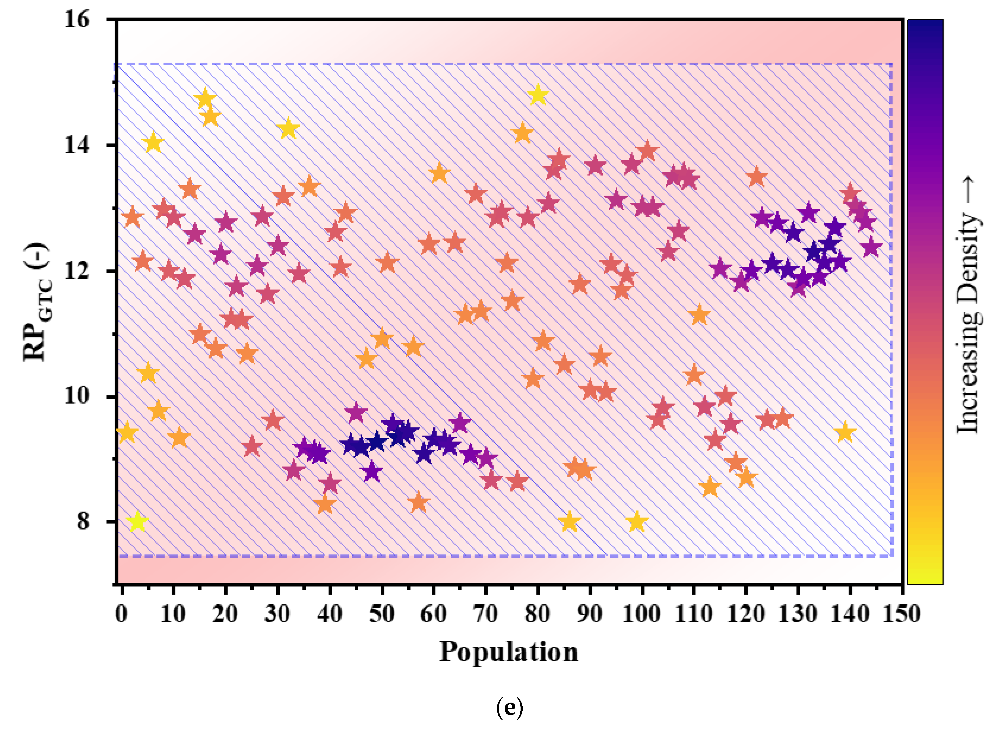
From the initial optimization process, Figure 8a–e illustrate the scattered distribution of decision variables (RPSCO2, CETDHE2, CETDHE3, T3, and RPGTC) within the optimal operational range. As the optimization purpose, this figure shows that the optimal values for decision variables, including RPSCO2, CETDHE2, CETDHE3, T3, and RPGTC, fall within the ranges of 1.8–2.8, 30–40 K, 50–30 K, 1450–1600 K, and 15–9, respectively.
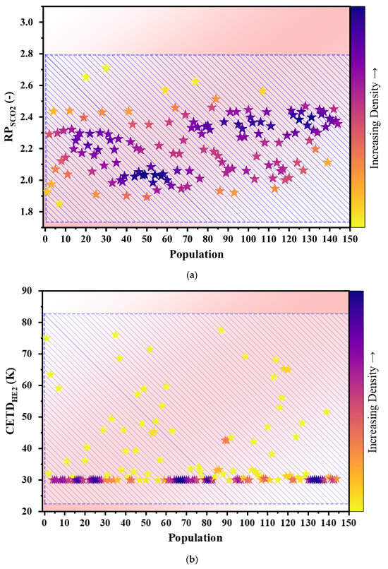
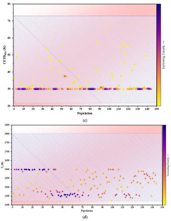
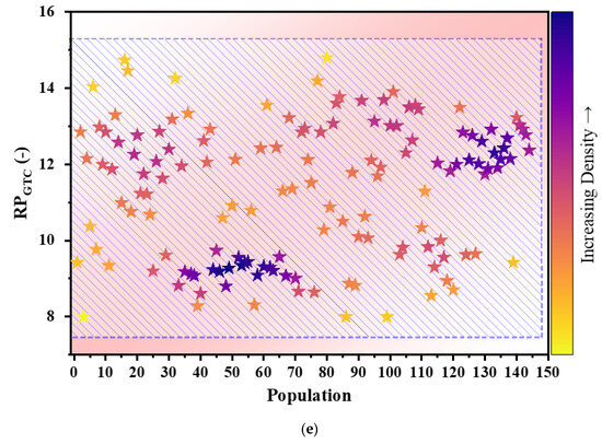
Figure 8.
(a) Scattered distribution for RPSCO2. (b) Scattered distribution for CETDHE2. (c) Scattered distribution for CETDHE3. (d) Scattered distribution for T3. (e) Scattered distribution for RPGTC.
6. Conclusions
The present study assesses a novel system for the simultaneous production of electric power and fresh water, comprising gas turbine subsystems with gasification processes, Brayton recondensation utilizing a supercritical carbon dioxide working fluid, organic Rankine cycle, and reverse osmosis. This system is assessed from energy, exergy, thermoeconomic, and environmental perspectives, and two distinct multi-objective optimization scenarios are applied featuring various objective functions. This simultaneous production system entails three power-producing subsystems and one fresh water-producing subsystem. Here, we outline the key findings derived from the study and the conclusions drawn from them:
- At the design point, the system has an exergy efficiency of 37.24%, a carbon dioxide emission index of 0.8977 kg/kWh, a unit cost of exergy products of 24.31 USD/GJ, a mass flow rate of produced fresh water of 42/61 kg/s, a total exergy destruction rate of 11,398 kW, and a net power production of 7347 kW.
- The parametric study shows that increasing the gas turbine pressure ratio results in escalating total unit cost of exergy products, net output power, and exergy efficiency initially, followed by a subsequent decline, while the mass flow rate of fresh water produced exhibits an opposite trend.
- Altering the pressure ratio of the Brayton recondensation subsystem utilizing supercritical carbon dioxide working fluid initially enhanced net output power, fresh water mass flow rate, and exergy efficiency before undergoing a decrease, while the unit cost of exergy products displays an initial reduction followed by an increase.
- Elevating the temperature difference of the cold terminal of heat exchanger 2 from 30 K to 80 K leads to linear increases in exergy efficiency, net power output, and fresh water mass flow, coupled with a linear decrease in the cost of exergy unit of products.
- Increasing the temperature difference of the cold terminal of heat exchanger 3 leads to a reduction in exergy efficiency, net output power, and mass flow rate of fresh water production, with the unit cost of exergy products exhibiting an initial decline followed by a rise.
- Gas turbine inlet temperature exhibits a direct relationship with exergy efficiency and net output power, and an inverse correlation with the mass flow rate of fresh water produced. Furthermore, raising the inlet temperature of the gas turbine from 1200 K to 1600 K initially leads to a decrease followed by a rise in the unit cost of exergy products of the system.
- In the first optimization scenario, considering the pollution index, total unit cost of exergy products, and exergy efficiency as objective functions, the optimal values are, respectively, identified as 0.7644 kg/kWh, 32.7 USD/GJ, and 44%. Conversely, in the second optimization scenario, featuring the emission index, total unit cost of exergy products, and output net power as objective functions, optimal values are 0.7684 kg/kWh, 27.82 USD/GJ, and 2615.9 kW.
Based on the findings, further research appears to be merited on this topic, including life cycle analysis for better environmental assessments and advanced exergy and exergoeconomic analyses for better thermodynamic and economic understanding.
Author Contributions
Conceptualization, F.P.G., N.G., S.S. and M.A.R.; Methodology, F.P.G., S.S.L., S.S. and M.A.R.; Software, F.P.G., S.S.L., N.G., S.S. and M.A.R.; Validation, F.P.G., S.S.L., N.G., S.S. and M.A.R.; Formal analysis, F.P.G., S.S.L., N.G., S.S. and M.A.R.; Investigation, F.P.G., S.S.L., N.G., S.S. and M.A.R.; Resources, F.P.G., S.S.L., N.G., S.S. and M.A.R.; Data curation, Saeed Soltani; Writing—original draft, F.P.G., S.S.L., N.G., S.S. and M.A.R.; Visualization, Saeed Soltani; Supervision, S.S. and M.A.R. All authors have read and agreed to the published version of the manuscript.
Funding
This research received no external funding.
Data Availability Statement
No new data were created or analyzed in this study.
Conflicts of Interest
The authors declare no conflict of interest.
Abbreviations
| AC | Air compressor |
| BPu | Boost pump |
| c | Cost per exergy unit, USD/GJ |
| cp,tot | Total product unit cost, USD/GJ |
| C | Compressor |
| CC | Combustion chamber |
| Cond | Condenser |
| CRF | Capital recovery factor |
| Cost rate, USD/h | |
| Exergy rate, kW | |
| FPu | Feed pump |
| fk | Exergoeconomic factor |
| GT | Gas turbine |
| GTIT | Gas turbine inlet temperature, K |
| h | Specific enthalpy, kJ/kg |
| HE | Heat exchanger |
| HPPu | High-pressure pump |
| HTR | High-temperature recuperator |
| IPCC | Intergovernmental Panel on Climate Change |
| K | Equilibrium constant |
| LHV | Higher heating value, kJ/kg |
| LTR | Low temperature recuperator |
| Mass flow rate, kg/s | |
| ORC | Organic Rankine cycle |
| P | Pressure, kPa |
| PT | Pelton turbine |
| Heat rate, MW | |
| REC | Recompression compressor |
| Reg | Regenerator |
| RES | Renewable energy sources |
| RO | Reverse osmosis |
| rp | Pressure ratio |
| rk | Relative cost difference |
| sCO2 | Supercritical carbon dioxide |
| ST | Steam turbine |
| STORC | Series of two-stage organic Rankine cycles |
| T | Temperature, K |
| Tg | Gasifier’s temperature, K |
| Work rate done/absorbed, MW | |
| Salt water mass fraction | |
| Purchased equipment cost, USD/h | |
| ηis | Isentropic efficiency |
| ζ | Carbon dioxide emission index |
| Ɛ | Effectiveness |
| ∅r | Maintenance factor |
| CI | Capital investment |
| OM | Repair and maintenance |
| g | Gasifier |
| is | Isentropic |
| in | Inlet |
| out | Outlet |
| D | Destroyed |
| 1, 2, … 42 | Numbers of states |
References
- Wang, L.; Wang, L.; Li, Y.; Wang, J. A century-long analysis of global warming and earth temperature using a random walk with drift approach. Decis. Anal. J. 2023, 7, 100237. [Google Scholar] [CrossRef]
- Akan, T. Can renewable energy mitigate the impacts of inflation and policy interest on climate change? Renew. Energy 2023, 214, 255–289. [Google Scholar] [CrossRef]
- Esily, R.R.; Yuanying, C.; Ibrahiem, D.M.; Houssam, N.; Makled, R.A.; Chen, Y. Environmental benefits of energy poverty alleviation, renewable resources, and urbanization in North Africa. Util. Policy 2023, 82, 101561. [Google Scholar] [CrossRef]
- Senegačnik, A.; Stropnik, R.; Sekavčnik, M.; Oprešnik, S.R.; Mlakar, U.; Ivanjko, Š.; Stritih, U. Integration of renewable energy sources for sustainable energy development in Slovenia till 2050. Sustain. Cities Soc. 2023, 96, 104668. [Google Scholar] [CrossRef]
- Gul, E.; Baldinelli, G.; Bartocci, P.; Shamim, T.; Domenighini, P.; Cotana, F.; Wang, J.; Fantozzi, F.; Bianchi, F. Transition toward net zero emissions—Integration and optimization of renewable energy sources: Solar, hydro, and biomass with the local grid station in central Italy. Renew. Energy 2023, 207, 672–686. [Google Scholar] [CrossRef]
- Ioannidis, F.; Kosmidou, K.; Papanastasiou, D. Public awareness of renewable energy sources and Circular Economy in Greece. Renew. Energy 2023, 206, 1086–1096. [Google Scholar] [CrossRef]
- Algarni, S.; Tirth, V.; Alqahtani, T.; Alshehery, S.; Kshirsagar, P. Contribution of renewable energy sources to the environmental impacts and economic benefits for sustainable development. Sustain. Energy Technol. Assess. 2023, 56, 103098. [Google Scholar] [CrossRef]
- Kocak, E.; Ulug, E.E.; Oralhan, B. The impact of electricity from renewable and non-renewable sources on energy poverty and greenhouse gas emissions (GHGs): Empirical evidence and policy implications. Energy 2023, 272, 127125. [Google Scholar] [CrossRef]
- Zabat, L.H.; Akli Sadaoui, N.; Abid, M.; Sekrafi, H. Threshold effects of renewable energy consumption by source in U.S. economy. Electr. Power Syst. Res. 2022, 213, 108669. [Google Scholar] [CrossRef]
- Fakudze, S.; Chen, J. A critical review on co-hydrothermal carbonization of biomass and fossil-based feedstocks for cleaner solid fuel production: Synergistic effects and environmental benefits. Chem. Eng. J. 2023, 457, 141004. [Google Scholar] [CrossRef]
- Verma, S.; Dregulo, A.M.; Kumar, V.; Bhargava, P.C.; Khan, N.; Singh, A.; Sun, X.; Sindhu, R.; Binod, P.; Zhang, Z.; et al. Reaction engineering during biomass gasification and conversion to energy. Energy 2023, 266, 126458. [Google Scholar] [CrossRef]
- Wang, J.; Fu, J.; Zhao, Z.; Bing, L.; Xi, F.; Wang, F.; Dong, J.; Wang, S.; Lin, G.; Yin, Y.; et al. Benefit analysis of multi-approach biomass energy utilization toward carbon neutrality. Innovation 2023, 4, 100423. [Google Scholar] [CrossRef] [PubMed]
- Ghorbani, S.; Atashkari, K.; Borji, M. Three-stage model-based evaluation of a downdraft biomass gasifier. Renew. Energy 2022, 194, 734–745. [Google Scholar] [CrossRef]
- Drobniak, A.; Jelonek, Z.; Mastalerz, M.; Jelonek, I. Residential gasification of solid biomass: Influence of raw material on emissions. Int. J. Coal Geol. 2023, 271, 104247. [Google Scholar] [CrossRef]
- Ngamsidhiphongsa, N.; Limleamthong, P.; Chalermsinsuwan, B.; Prasertcharoensuk, P.; Wiyaratn, W.; Arpornwichanop, A. Application of computational fluid dynamics and response surface methodology in downdraft gasification using multiple biomass pellets. J. Clean. Prod. 2023, 417, 137923. [Google Scholar] [CrossRef]
- Batista, N.E.; Carvalho, P.C.M.; Fernández-Ramírez, L.M.; Braga, A.P.S. Optimizing methodologies of hybrid renewable energy systems powered reverse osmosis plants. Renew. Sustain. Energy Rev. 2023, 182, 113377. [Google Scholar] [CrossRef]
- Zubair, M.M.; Saleem, H.; Zaidi, S.J. Recent progress in reverse osmosis modeling: An overview. Desalination 2023, 564, 116705. [Google Scholar] [CrossRef]
- Kolathur, S.; Khatiwada, D.; Khan, E.U. Life cycle assessment and life cycle costing of a building-scale, solar-driven water purification system. Energy Nexus 2023, 10, 100208. [Google Scholar] [CrossRef]
- Alawad, S.M.; Mansour, R.B.; Al-Sulaiman, F.A.; Rehman, S. Renewable energy systems for water desalination applications: A comprehensive review. Energy Convers. Manag. 2023, 286, 117035. [Google Scholar] [CrossRef]
- Javaherian, A.; Yari, M.; Gholamian, E.; Carton, J.G.; Mehr, A.S. Proposal and comprehensive analysis of power and green hydrogen production using a novel integration of flame-assisted fuel cell system and Vanadium-Chlorine cycle: An application of multi-objective optimization. Energy Convers. Manag. 2023, 277, 116659. [Google Scholar] [CrossRef]
- Ahmad, A.A.; Zawawi, N.A.; Kasim, F.H.; Inayat, A.; Khasri, A. Assessing the gasification performance of biomass: A review on biomass gasification process conditions, optimization and economic evaluation. Renew. Sustain. Energy Rev. 2016, 53, 1333–1347. [Google Scholar] [CrossRef]
- Li, Y.; Zhang, L.; Zhao, W.; Song, X.; Wei, J.; Bai, Y.; Wang, J.; Yu, G. Biomass erosion and its effect on heat carrying performance of alumina heat carrier during multiple cycle sintering in solar photothermal coupled with biomass gasification. Chem. Eng. Sci. 2024, 120807. [Google Scholar] [CrossRef]
- Yilmaz, F.; Ozturk, M.; Selbas, R. Design and thermodynamic assessment of a biomass gasification plant integrated with Brayton cycle and solid oxide steam electrolyzer for compressed hydrogen production. Int. J. Hydrog. Energy 2020, 45, 34620–34636. [Google Scholar] [CrossRef]
- Chen, H.; Lu, D.; An, J.; Qiao, S.; Dong, Y.; Jiang, X.; Xu, G.; Liu, T. Thermo-Economic analysis of a novel biomass Gasification-Based power system integrated with a supercritical CO2 cycle and a Coal-Fired power plant. Energy Convers. Manag. 2022, 266, 115860. [Google Scholar] [CrossRef]
- Roy, D. Multi-objective optimization of biomass gasification based combined heat and power system employing molten carbonate fuel cell and externally fired gas turbine. Appl. Energy 2023, 348, 121486. [Google Scholar] [CrossRef]
- Blanco-Marigorta, A.M.; Masi, M.; Manfrida, G. Exergo-environmental analysis of a reverse osmosis desalination plant in Gran Canaria. Energy 2014, 76, 223–232. [Google Scholar] [CrossRef]
- Abbasi, H.R.; Pourrahmani, H. Multi-objective optimization and exergoeconomic analysis of a continuous solar-driven system with PCM for power, cooling and freshwater production. Energy Convers. Manag. 2020, 211, 112761. [Google Scholar] [CrossRef]
- Nemati, A.; Sadeghi, M.; Yari, M. Exergoeconomic analysis and multi-objective optimization of a marine engine waste heat driven RO desalination system integrated with an organic Rankine cycle using zeotropic working fluid. Desalination 2017, 422, 113–123. [Google Scholar] [CrossRef]
- Abdolalipouradl, M.; Mohammadkhani, F.; Khalilarya, S.; Yari, M. Thermodynamic and exergoeconomic analysis of two novel tri-generation cycles for power, hydrogen and freshwater production from geothermal energy. Energy Convers. Manag. 2020, 226, 113544. [Google Scholar] [CrossRef]
- Pan, M.; Zhu, Y.; Bian, X.; Liang, Y.; Lu, F.; Ban, Z. Theoretical analysis and comparison on supercritical CO2 based combined cycles for waste heat recovery of engine. Energy Convers. Manag. 2020, 219, 113049. [Google Scholar] [CrossRef]
- Song, J.; Wang, Y.; Wang, K.; Wang, J.; Markides, C.N. Combined supercritical CO2 (SCO2) cycle and organic Rankine cycle (ORC) system for hybrid solar and geothermal power generation: Thermoeconomic assessment of various configurations. Renew. Energy 2021, 174, 1020–1035. [Google Scholar] [CrossRef]
- Khoshgoftar Manesh, M.H.; Firouzi, P.; Kabiri, S.; Blanco-Marigorta, A.M. Evaluation of power and freshwater production based on integrated gas turbine, S-CO2, and ORC cycles with RO desalination unit. Energy Convers. Manag. 2021, 228, 113607. [Google Scholar] [CrossRef]
- Wang, S.; Liu, C.; Li, J.; Sun, Z.; Chen, X.; Wang, X. Exergoeconomic analysis of a novel trigeneration system containing supercritical CO2 Brayton cycle, organic Rankine cycle and absorption refrigeration cycle for gas turbine waste heat recovery. Energy Convers. Manag. 2020, 221, 113064. [Google Scholar] [CrossRef]
- Soltani, S.; Mahmoudi, S.M.S.; Yari, M.; Rosen, M.A. Thermodynamic analyses of a biomass integrated fired combined cycle. Appl. Therm. Eng. 2013, 59, 60–68. [Google Scholar] [CrossRef]
- Zainal, Z.A.; Ali, R.; Lean, C.H.; Seetharamu, K.N. Prediction of performance of a downdraft gasifier using equilibrium modeling for different biomass materials. Energy Convers. Manag. 2001, 42, 1499–1515. [Google Scholar] [CrossRef]
- Bejan, A.; Tsatsaronis, G.; Moran, M.J. Thermal Design and Optimization; Wiley: Wiley-Interscience Publication: Hoboken, NJ, USA, 1995; ISBN 9780471584674. [Google Scholar]
- Moharramian, A.; Soltani, S.; Rosen, M.A.; Mahmoudi, S.M.S.; Jafari, M. Conventional and enhanced thermodynamic and exergoeconomic analyses of a photovoltaic combined cycle with biomass post firing and hydrogen production. Appl. Therm. Eng. 2019, 160, 113996. [Google Scholar] [CrossRef]
- Javaherian, A.; Ghasemzadeh, N.; Javanshir, N.; Yari, M.; Vajdi, M.; Nami, H. Techno-environmental assessment and machine learning-based optimization of a novel dual-source multi-generation energy system. Process Saf. Environ. Prot. 2023, 176, 537–559. [Google Scholar] [CrossRef]
Disclaimer/Publisher’s Note: The statements, opinions and data contained in all publications are solely those of the individual author(s) and contributor(s) and not of MDPI and/or the editor(s). MDPI and/or the editor(s) disclaim responsibility for any injury to people or property resulting from any ideas, methods, instructions or products referred to in the content. |
© 2024 by the authors. Licensee MDPI, Basel, Switzerland. This article is an open access article distributed under the terms and conditions of the Creative Commons Attribution (CC BY) license (https://creativecommons.org/licenses/by/4.0/).


