Spatial and Temporal Evolution Characteristics of Ecosystem Service Value and Population Distribution in China’s Coastal Areas

Abstract

Coastal areas are among the most densely populated areas globally and are crucial components of terrestrial and marine ecosystems. Investigating the interplay between population distribution and the ecosystem service value (ESV) in coastal regions, along with their spatial and temporal dynamics, is crucial for safeguarding coastal ecological security, fostering regional sustainable development, and facilitating a harmonious coexistence between humans and nature. This study focuses on China’s coastal areas, utilizing land use and population data from 2000 to 2020 at the county-level scale. Several methods, such as geographic concentration, spatial autocorrelation, and the spatial mismatch index, are employed to reveal the relationships and spatial and temporal characteristics between population and the ESV. The main findings are as follows: (1) The population in China’s coastal areas increased from 580.6632 million to 700.7265 million, with a rising population density. The population distribution core is concentrated in the Beijing–Tianjin–Hebei Urban Agglomeration, the Yangtze River Delta Urban Agglomeration, and the Pearl River Delta Urban Agglomeration, with secondary cores forming near provincial capitals. (2) The ecological geographic concentration in China’s coastal areas is lower than that of the population, displaying a distribution pattern of “low–high–low” from north to south. The ESV in these areas has increased by CNY 121.66 billion, with a significant decline in the per capita ESV. Low values of ecological geographic concentrations are concentrated in the northern part of the research area, particularly across the North China Plain. (3) The correlation between the ESV and population in China’s coastal areas is negative, with relatively good overall coordination. Increased human activities and urbanization in the Yangtze River Delta and Pearl River Delta have led to the degradation of ecological functions.

1. Introduction

In 2015, the United Nations introduced the Sustainable Development Goals (SDGs) to address social, economic, and environmental development issues comprehensively. Ecosystem services are closely related to environmental development. Ecosystem services refer to the natural environmental conditions and functions that are formed and maintained through the interactions between ecosystems and human survival processes. These services include provisioning services (such as food, freshwater, and fuel), regulating services (such as climate regulation, water purification, and pollination), cultural services (such as recreation, cultural heritage, and esthetic value), and supporting services (such as soil formation and habitat provision) [1]. Ecosystem services are essential for human survival and serve as fundamental guarantees for achieving ecological security [2]. From an ecological economics perspective, the direct use value of ecosystem services is often emphasized during human development and utilization, whereas the derived external ecological benefits are neglected [3]. This has led to a decline in the capacity of ecosystem service provision, resulting in various issues, such as fragmented ecological patterns and loss of biodiversity. Costanza et al. (1997) scientifically explained the principles and methods for estimating the ecosystem service value (ESV) [4]. Since then, the ESV has been widely researched globally and has become a prominent and cutting-edge issue in global or regional organizations and the scientific community [5]. Scholars have explored the impact of land use changes on the ESV at various scales, such as the regional, watershed, and national levels [6,7,8]. Ecosystems are also influenced by human activities [9]. Human activities have a significant impact on changes in ecosystem service values [10], with over 60% of global ecosystems undergoing or having already undergone degradation [11] and with 1/3 to 1/2 of the land surface being altered by human activities [12].

Economic activities are generally attracted to the ocean as a common pattern of social development [13]. Coastal ecosystems play irreplaceable roles in material production, climate regulation, water source protection, pollutant removal, and biodiversity maintenance, making them among the most valuable natural ecosystems on Earth. However, over half of the global population, production, and consumption activities are concentrated in coastal areas that cover less than 10% of the Earth’s surface [14], with over 40% of the oceans being strongly affected by various anthropogenic factors. Even polar regions are impacted by human activities [15]. This has led to a series of ecological and environmental issues, prominently including the destruction of the structure and components of natural ecosystems and the weakening or loss of ecosystem services. Therefore, the role, pattern, and mechanism of human–environment interactions in coastal areas have become key focuses of relevant research [16].

Human activities are significant drivers of changes in ecosystem services [17,18]. With the increase in human activities, such as agricultural production and urban construction, the types of land use have undergone rapid changes [19]. Irrational land use disrupts ecosystem services by affecting energy flow and material cycling in ecosystems [20]. Numerous results have been obtained in studies related to the impact of anthropogenic intensity on ESVs [21,22,23], such as ecosystem service management and trade-offs [24,25], human activity intensity [26,27], and ecological policy benefits [28,29]. Research methods for calculating the ESV mainly include equivalent factor methods [30,31] and functional value methods [32], with analyses of correlation [33,34,35], spatial regression models, etc., to explore the relationships between them. Li et al. (2019) used remote sensing images from two periods and ecological assessment methods to investigate the impact of human activities on the ESV [23]. Gao et al. (2021) focused on an ESV spatial and temporal analysis and ecological compensation in the Taihu Basin, with a focus on population as an ecological compensation subject [36]. However, as a direct indicator of human activity intensity, population has either been overlooked or used only as a single evaluation metric in existing studies, failing to reveal the coordination and spatial and temporal characteristics between ecosystem services and population.

Therefore, this study selects China’s coastal areas as the research area, focusing on the interaction between population and the ESV. It analyses the spatial and temporal changes in population and the ESV in 2000, 2010, and 2020, explores the spatial differentiation characteristics, patterns, and driving factors, and reveals the correlation and coordination between population and the ESV. Research on the spatial and temporal evolution of population and the ESV in China’s coastal areas can provide valuable references and important case studies for the sustainable development of coastal areas worldwide.

2. Materials and Methods

2.1. Research Area

The research area is coastal areas along China’s mainland coastline, with a total length of approximately 15,780 km, encompassing 11 provinces, including Beijing, Liaoning, Hebei, Tianjin, Shandong, Jiangsu, Shanghai, Zhejiang, Fujian, Guangdong, and Guangxi (excluding Hong Kong, Macao, and Taiwan), and 1068 county-level units (Figure 1). The coastal areas of China house the country’s most significant urban agglomerations (the Beijing–Tianjin–Hebei Urban Agglomeration, the Yangtze River Delta Urban Agglomeration, and the Guangdong–Hong Kong–Macao Greater Bay Area). These areas represent the most economically developed, densely populated, and highly frequented areas, accounting for 12.59% of China’s total land area. According to the Seventh Population Census of China, the population in these regions totals approximately 646 million, or 46.81% of the country’s total population. Urbanization, population agglomeration, port construction, mariculture, and other human activities have altered the coastline morphology and tidal patterns of China’s coastal areas, disrupting the original ecological balance and exerting profound impacts on ecosystem services in the area.

2.2. Research Methods

2.2.1. ESV Evaluation

On the basis of the revised ecosystem service equivalency table by Xie et al. (2015) [1], this study also refers to the unit area ecosystem service values from Xie et al. (2008) [37] and Xu et al. (2012) [38]. The standard equivalent factor is determined via the average net profit per unit area of three main crops (rice, wheat, and corn) from 2000 to 2015, which is 2181.78 CNY/hm² [39]. Finally, the unit area ecosystem service value table for different land use types is obtained (

Table 1. Coefficients of the value of ecosystem services of various types of land (CNY/ha/yr).

Primary Type	Secondary Type	Farmland	Forest	Grassland	Water Area	Unused Land
Provision Services	Food Production	2421.78	545.45	501.81	1745.42	21.82
	Raw Material Production	545.45	1265.43	741.81	501.81	43.64
	Water Resource Supply	−2858.13	654.53	414.54	18,086.96	21.82
Regulatory Services	Gas Regulation	1941.78	4167.20	2639.95	1679.97	152.72
	Climate Regulation	1025.44	12,457.96	6959.88	4996.28	109.09
	Environmental Purification	305.45	3643.57	2290.87	12,108.88	458.17
	Hydrological Regulation	3272.67	8159.86	5105.37	223,065.19	261.81
Support Services	Soil Conservation	1134.53	5061.73	3207.22	2029.06	174.54
	Nutrient Cycling Maintenance	349.08	392.72	240.00	152.72	21.82
	Biodiversity	370.90	4625.37	2923.59	5563.54	152.72
Cultural Services	Esthetic Landscape	174.54	2029.06	1287.25	4123.56	65.45

), with the service value coefficient for construction land set to 0. The ESV calculation formula is as follows:

$$ESV=\sum _{\dot{i}=1}^n(A_i\times V{C}_i)$$

(1)

where ESV is the ecosystem service value of the research area; A_i is the area of the ith land type in the research area; VC_i is the ecosystem service value coefficient for the ith land type; and n is the number of land types.

2.2.2. Geographical Concentration

This study uses geographical concentration to analyze the spatial characteristics of population and ecosystem service values [40]. The calculation formulas are as follows:

$$R_{PO{P}_i}={\displaystyle \frac{PO{P}_i/POP}{S_i/S}}$$

(2)

$$R_{ES{V}_i}={\displaystyle \frac{ES{V}_i/ESV}{S_i/S}}$$

(3)

where R_POPi and R_ESVi represent the geographical concentrations of the population and ecosystem services in unit i, respectively. The magnitude reflects the degree of spatial concentration, with higher values indicating greater concentrations. POP, ESV_i, and S_i represent the total population, total ecosystem service value, and total area of the research area, respectively.

2.2.3. Kernel Density Estimation

Kernel density estimation is a nonparametric method for studying data distribution characteristics by using the data themselves as the subject of analysis without any assumptions about the data distribution. This avoids errors that might arise from unreasonable assumptions. Compared with histograms, it is more intuitive and conceptually simple [41]. The formula is as follows:

$$f\left(s\right)={\displaystyle \frac{1}{nr}}\sum _{i=1}^{n}k\left({\displaystyle \frac{d_{is}}{r}}\right)$$

(4)

where f(s) is the density at location S, n is the number of samples that fall within the search radius, d_is is the distance from point i to s, k is the kernel function for d_is and r, and r is the bandwidth, which is the search radius. The density distribution is highest at each central point and decreases outwards, becoming zero after a certain range. We used the default settings in the ArcGIS kernel density estimation tool.

2.2.4. Trend Surface Analysis

Trend surface analysis fits a global polynomial to spatial sample points, converting two-dimensional spatial data into a three-dimensional smooth curve to visualize the spatial trends of geographical features. This study uses trend surfaces to represent spatial variation trends in population and ecosystem service values in coastal areas. The formula is as follows [42]:

$$z_i\left(x_i,y_i\right)={\widehat{z}}_i\left(x_i,y_i\right)+{\epsilon }_i$$

(5)

where (x_i, y_i) are geographical coordinates, $z_i\left(x_i,y_i\right)$ is the real surface, ${\widehat{z}}_i\left(x_i,y_i\right)$ is the fitted surface, and ε_i represents residuals, i.e., the deviation between actual and fitted values. We use the two-dimensional minimum curvature spline technique to interpolate raster surfaces from points, with a default weight of 0.1.

2.2.5. Exploratory Spatial Data Analysis

This study uses exploratory spatial data analysis to identify anomalies in population and ESV spatial data and reveal the spatial interaction mechanisms [43] between the two. This includes global spatial autocorrelation and local spatial autocorrelation [44]. Univariate spatial autocorrelation is used to study the spatial clustering characteristics of population geographical concentration and eco-geographic concentration, whereas bivariate spatial autocorrelation is used to study the spatial association features of the two [45]. The calculation formula is as follows:

$$I={\displaystyle \frac{{\sum }_{i=1}^n{\sum }_{j=1}^n{w}_{ij}\left(x_i-\overline{x}\right)\left(y_j-\overline{y}\right)}{s^2{\sum }_{i=1}^n{\sum }_{j=1}^n{w}_{ij}}}$$

(6)

where I is the bivariate global Moran index, which represents the overall spatial distribution correlation between the independent variable of unit i and the dependent variable of unit j; x_i and y_i represent the observations of different geographical entities for units i and j, respectively; n is the number of units; w_ij is the spatial adjacency weight matrix for units i and j; and s² is the sample variance.

The formula for calculating the bivariate local spatial autocorrelation is as follows:

$$I_i={\displaystyle \frac{\left(x_i-\overline{x}\right)}{s^2}}\sum _{j=1}^n{w}_{ij}\left(y_j-\overline{y}\right)$$

(7)

where I_i represents the local spatial association between the independent variable and the dependent variable at unit i. The results can categorize each unit into four types, namely H–H (high–high), L–L (low–low), H–L (high–low), and L–H (low–high).

2.2.6. Spatial Mismatch Index

Owing to the spatial distribution differences between population and ecosystem service values (ESVs) within the research area, the spatial mismatch index is used to reflect the distribution disparity between the two. The calculation formula is as follows:

$$SM{I}_i={\displaystyle \frac{1}{POP}}\left[\right({\displaystyle \frac{ES{V}_i}{ESV}})POP-PO{P}_i]\times 100$$

(8)

where SMI_i represents the spatial mismatch intensity of population and the ESV at unit i. If SMI_i is positive, it indicates that the ESV level at that unit exceeds the population, meaning that there is a surplus of the ESV; if it is negative, the opposite result is true. The smaller the absolute value is, the lower the spatial mismatch index and the higher the degree of coordination (

Table 2. Population and ESV coordination typology.

Standard	Type	Category	Coordination Type
SMIi ≤ −1	Negative high mismatch area	Population significantly ahead of ESV level	ESV level lags behind population demand, uncoordinated
−1 < SMIi ≤ −0.2	Negative moderate mismatch area	Population slightly ahead of ESV level
−0.2 < SMIi ≤ 0	Negative low mismatch area	Population roughly matches ESV level	Coordinated city
0 < SMIi ≤ 0.2	Positive low mismatch area
0.2 < SMIi ≤ 1	Positive moderate mismatch area	Population slightly behind ESV level	ESV level ahead of population demand, uncoordinated
SMIi > 1	Positive moderate and high area	Population significantly behind ESV level

).

2.3. Data Sources

The land use data in this study (for 2000, 2010, and 2020) come from the Resource and Environmental Science Data Platform (https://www.resdc.cn, accessed on 18 September 2024), with a spatial resolution of 30 m × 30 m. The population data in this study come from the fifth, sixth, and seventh national population censuses of China, with population counts for each county and district representing the local resident population. Population censuses are conducted every ten years in China, making these data the most accurate and authoritative. Administrative division data are sourced from the National Geomatics Center of China (http://ngcc.sbsm.gov.cn/, accessed on 18 September 2024), with administrative division adjustments based on the data for the relevant municipal cities for each year.

3. Results and Analysis

3.1. Spatial and Temporal Changes in Population

3.1.1. Spatial and Temporal Changes in Population Density

The total population in China’s coastal areas was 580.6632 million in 2000, 647.6572 million in 2010, and 700.7265 million in 2020. Over the 20-year period, the population increased by 120.0633 million, with an average annual growth rate of approximately 20.68%. The population density increased from 1190.06 person/km² in 2000 to 1450.19 person/km² in 2010 and to 1673.25 person/km² in 2020. The density trend is increasing, although it is unevenly distributed across different regions. The most notable increases in population density occurred in the Beijing–Tianjin–Hebei Urban Agglomeration, the Yangtze River Delta Urban Agglomeration, and the Pearl River Delta Urban Agglomeration. The data were divided into 10 quantiles and rounded where possible [46]. High-population-density areas are concentrated in provincial capitals and their surroundings, such as the Nanjing–Shanghai region (Yangtze River Delta), the Shanghai–Hangzhou–Ningbo region (Hangzhou Bay), and the Guangzhou–Dongguan–Shenzhen region (Pearl River Delta), forming high-density cores that are either point-like or block-like (Figure 2). These regions are the most economically developed in China, with high urbanization rates, high per capita income, and numerous employment opportunities. A significant migration of the population from inland areas to coastal areas has occurred in search of non-agricultural work and increased income. This movement also includes periodic returns to inland areas, leading to large-scale population flow phenomena, such as the “spring festival travel rush”.

Compared with 2000, the number of high-population-density districts in coastal areas increased significantly by 2010. Populations from the central and western regions began migrating to the eastern coastal areas in search of better job opportunities. The attraction of the Yangtze River Delta Urban Agglomeration increased, with moderate-density-population areas around Hangzhou and Shanghai transitioning to higher-density categories (e.g., Tongxiang and Pinghu became higher-density areas, whereas Yuyao and Cixi transitioned to high-density categories). Additionally, districts near Fuzhou (e.g., Minhou) shifted from a low to moderate population density. Areas with rapid population growth are primarily those near urban centres. By 2020, the trend in high population density became even more pronounced around provincial capitals, with districts surrounding provincial capitals generally shifting to higher-density categories. The high-density core area from Shanghai southeast to Shenzhen has progressively covered the entire coastal district, indicating a trend in comprehensive coverage across the coastal areas.

3.1.2. Spatial and Temporal Changes in Population Geographic Concentration

On the basis of population geographic concentration values at the district and county scales, the levels are classified into five levels from low to high, at low, relatively low, moderate, high, and very high. The population geographic concentration in China’s coastal areas shows significant spatial variation (Figure 3a–c). Specifically, areas with relatively high population geographic concentrations are located mainly in the North China Plain, the Yangtze River Delta, the Pearl River Delta, and around provincial capital cities, such as Nanning and Shenyang. In contrast, the inland districts and counties in Guangxi, Guangdong, Fujian, Zhejiang, Hebei, and Liaoning have relatively lower population geographic concentrations. Several factors, such as mountainous terrain, shorter rivers, and relatively slow economic development, are important reasons for the lower population concentration in the inland areas of Zhejiang, Fujian, Guangdong, and Guangxi. Additionally, the population concentration in northern coastal areas is generally higher than that in southern coastal areas, with especially high concentration levels in the North China Plain (southern Hebei, Shandong, and northern Jiangsu).

From 2000 to 2020, population changes and geographic concentrations in China’s coastal areas exhibited considerable spatial variation (Figure 3d). In the districts and counties of the Yangtze River Delta and the Pearl River Delta, the population has been increasing. However, in most districts and counties of the North China Plain, where the population geographic concentration is high, the population has been decreasing. The districts and counties in the Pearl River Delta have relatively low population geographic concentrations. Major urban centres experiencing population growth include Beijing, Shanghai, Guangzhou, Shenzhen, and Nanjing, with increases also observed in the districts of Shenyang, Nanning, Fuzhou, Wenzhou, and Liuzhou. These findings suggest that the three major urban agglomerations in China (Beijing–Tianjin–Hebei, the Yangtze River Delta, and the Pearl River Delta) are likely to attract even larger populations in the future.

3.1.3. Population Spatial Structure and Trends

Through trend surface analysis, the spatial distribution patterns of the population can be observed more intuitively. The results of the trend surface fitting (Figure 4) indicate that the population density along China’s coastal areas shows a spatial orientation pattern of “high–low–high–low–high” from north to south, with significant peaks in three areas (Beijing, Shanghai, and Guangzhou). These locations are regions with relatively high population densities. To gain a deeper understanding of the spatial changes in population along China’s coastal areas, we created a county-level population density kernel map (Figure 5). This study reveals that the population distribution in China’s coastal areas has a distinct hierarchical structure characterized by a high-density distribution in the three major city clusters and localized concentrations around provincial capitals, whereas the inland areas present a scattered distribution pattern, which forms a high-density population distribution pattern centred on Beijing, Shanghai, and Guangzhou.

3.2. Spatial and Temporal Changes in Ecosystem Service Value (ESV)

3.2.1. Spatial and Temporal Changes in per Capita Ecosystem Service Value

The ESV in China’s coastal areas was CNY 4.197454 trillion in 2000, CNY 4.252453 trillion in 2010, and CNY 4.319114 trillion in 2020. Over the 20-year period, it increased by CNY 121.66 billion, with an annual growth rate of approximately 2.9%, which is lower than the annual population growth rate of 20.68%. Forests and water bodies constitute the majority of the ESV in China’s coastal areas, accounting for approximately 52% and 31%, respectively. This is followed by croplands and grasslands, which make up approximately 10% and 6%, respectively (

Table 3. Value of ecosystem services for various types of land in 2000, 2010, and 2020.

Unit: 108 CNY	Farmland	Forest	Grassland	Water	Unused Land	Total
2000	4314.18	22,388.65	2886.61	12,376.23	8.86	41,974.54
2010	4121.37	22,489.60	2548.09	13,357.81	7.65	42,524.53
2020	4057.13	22,196.59	2554.35	14,376.45	6.63	43,191.14
ESV change	−257.05	−192.06	−332.26	2000.22	−2.23	1216.6

). Among these, the ESV of water bodies increased by CNY 200.022 billion, whereas the ESVs of grasslands, croplands, forests, and unused lands decreased by CNY 33.226 billion, CNY 25.705 billion, CNY 19.206 billion, and CNY 0.223 billion, respectively. Hydrological regulation, climate regulation, and air purification are the main components of the ESV, with regulating services occupying a major position. Several functions, such as food production and nutrient cycling, need to be reinforced in the future (

Table 4. An evaluation of the values of the different types of ecosystem services in 2000, 2010, and 2020.

Ecosystem Classification		2000 (108 CNY)	2010 (108 CNY)	2020 (108 CNY)
Primary	Secondary
Supply services	Food	1621.18	1568.47	1553.43
	Materials	1034.12	1017.20	1006.55
	Water	−216.81	−92.38	−8.38
Regulating services	Air quality regulation	3500.70	3439.30	3403.30
	Climate regulation	7985.29	7920.03	7847.71
	Purifying environment	2849.61	2864.90	2883.05
	Regulation of water flows	16,509.49	17,189.03	17,939.37
Supporting services	Soil conservation	3643.48	3596.04	3561.34
	Maintain nutrient circulation	411.25	401.87	397.22
	Biodiversity	3165.29	3150.10	3137.11
Cultural service	Esthetic landscape	1470.94	1469.98	1470.45

).

The per capita ESV in China’s coastal areas has been declining, with figures of CNY 7228.72 (2000), CNY 6565.83 (2010), and CNY 6212.33 (2020). As shown in Figure 6a–c, there is significant regional differentiation in the per capita ESV; areas with lower per capita ESVs are concentrated in the North China Plain, coastal areas, and provincial capitals, whereas other areas have higher per capita ESVs. The main reasons for this regional differentiation are as follows: (1) The North China Plain, which is the primary agricultural area in China, has a high ratio of arable and construction land, resulting in a lower ESV. Coupled with a high population density, this leads to a lower per capita ESV in these areas. (2) In contrast, the region south of the Yangtze River, with more precipitation, higher temperatures, and denser river and lake networks, supports better vegetation growth, leading to higher per capita ESVs in these areas. (3) In northern Hebei Province and most of Liaoning Province, which are mountainous, population outflow and ecological forest construction have resulted in higher per capita ESVs in these counties. Further analysis of the annual growth rate of the per capita ESV from 2000 to 2020 (Figure 6d) reveals that areas with relatively high per capita ESV growth rates are located primarily in eastern and western Liaoning, with some scattered areas in Jiangsu, Fujian, and Guangxi. Areas with higher per capita ESV decline rates are concentrated in Beijing, Shenyang, Nanning, and Guangzhou. Population outflow is a key factor in the increase in the per capita ESV, particularly in economically lagging regions, such as Northeast China, northern Jiangsu, and northern Guangxi.

3.2.2. Spatial and Temporal Changes in Eco-Geographic Concentration

The eco-geographic concentration in China’s coastal areas displays a north–south high and central low distribution pattern (Figure 7a–c). High eco-geographic concentrations are observed in regions south of the Yangtze River, Changbai Mountain and Yan Mountain areas, along the Grand Canal’s Lake regions, and near the Yellow River estuary. Conversely, the North China Plain, Shandong Peninsula, and several cities, such as Shanghai and Yancheng, have relatively low eco-geographic concentrations. Among the different provinces within the Yangtze River Basin, Guangxi has lower eco-geographic concentrations than Guangdong, Fujian, and Zhejiang, primarily because of its extensive karst topography and abundant precipitation but limited surface water storage, resulting in more shrubland and grassland. The North China Plain (including Beijing, Tianjin, northern Jiangsu, western Shandong, and southern Hebei) is a major agricultural and urban area with frequent human activities, resulting in lower eco-geographic concentrations.

An analysis of the changes in eco-geographic concentration (Figure 7d) from 2000 to 2020 shows that 446 county units along China’s coast experienced a decline in eco-geographic concentration, with notable decreases in several regions, such as Guangzhou–Shenzhen, Shanghai–Nanjing, and Shenyang–Panjin. Conversely, 638 county units showed an increase in eco-geographic concentration, primarily in Guangxi, Guangdong, Liaoning, northern Jiangsu, and coastal Shandong.

3.2.3. Evolution of the Spatial Structure of Ecosystem Service Value

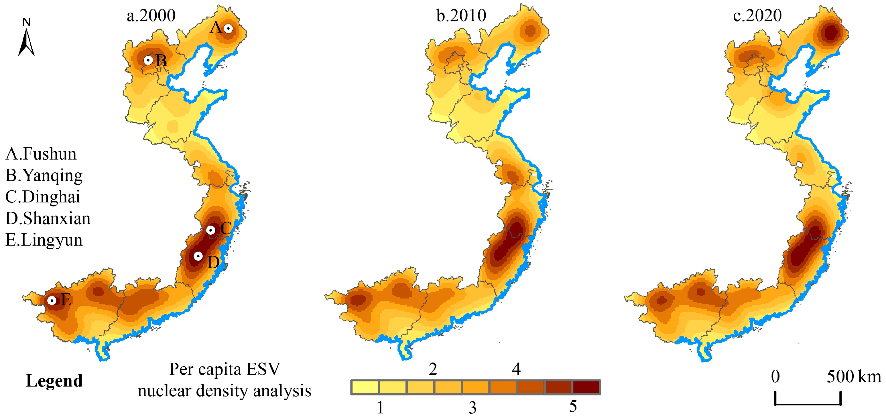
Unlike the curve fit for the permanent population, the per capita ESV trend surface exhibits a spatial distribution pattern of “low in the east, high in the west, low in the north, and high in the south” (Figure 8), indicating more pronounced spatial orientation characteristics. This study employs kernel density estimation to further reveal the regional differentiation pattern of the per capita ESV in China’s coastal areas (Figure 9).

The analysis indicates that from 2000 to 2020, the per capita ESV in China’s coastal areas was high in the north and south and low in the middle, similar to the pattern of the eco-geographic concentration distribution. Specifically, high values of the per capita ESV are mainly concentrated in southern Fujian and Zhejiang, with secondary high values in Guangxi, northern Guangdong, northern Hebei, and eastern Liaoning; low values are primarily found across the North China Plain (southern Hebei, Shandong, and northern Jiangsu) and coastal areas. By comparing the regional distribution characteristics of population density and ESV density, we observe a spatial mismatch between the two. To explore the reasons behind this phenomenon, a follow-up analysis of the coordination between the two was conducted.

3.3. Coordination Between Population and Ecosystem Service Value

3.3.1. Spatial Correlation Characteristics

The Spearman correlation coefficients for the geographical concentration of the ESV and population in 2000, 2010, and 2020 were −0.125, −0.159, and −0.151, respectively, indicating a negative correlation between the two. The bivariate global Moran indices were −0.103, −0.125, and −0.119, suggesting a negative spatial association between eco-geographic concentration and population geographic concentration.

In terms of the spatial distribution of aggregation types, relatively few high (eco-geographic concentration)–high (population geographic concentration) counties, such as Qingyuan, Gaochun, Kaihua, and Wuyishan, are distributed as isolated points (Figure 10). These counties have a relatively high proportion of forest or water areas, such as national forest parks (Wuyishan), lakes and reservoirs (Wuyishan, Gaochun), and Hunan Forest Park (Qingyuan), providing significant ecosystem service value. Moreover, these counties have a high level of urbanization and a relatively high population density. The highest number of counties falls into the high-ESV and low-population category, totaling 139 in 2020. This type is distributed in a band-like pattern and is found mainly in Guangxi, Guangdong, Fujian, Zhejiang, and parts of Liaoning and Hebei. Fewer low-ESV and high-population counties are located in areas farther from the coast, such as Caoxian, Pukou, and Xilin. The number of low-ESV and low-population counties increased from 66 in 2000 to 86 in 2020, mainly around Nanning, Liuzhou, Zhangjiakou, Dongying, and Fuxin. These areas were once more urbanized with higher populations but have experienced population decline over time.

3.3.2. Coordination Between Population and Total ESV

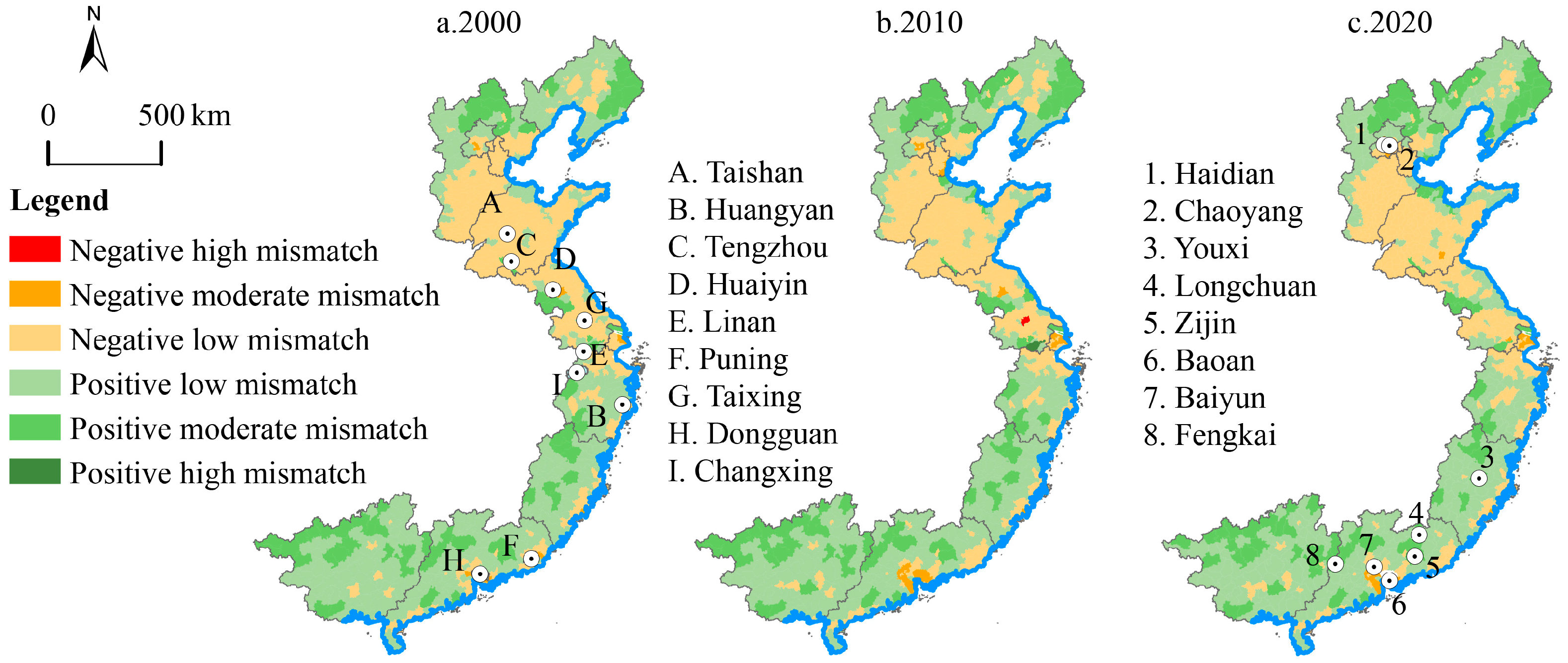
On the basis of bivariate spatial autocorrelation analysis, the spatial mismatch index was further used to analyze the types, intensities, and evolution characteristics of errors between population and the ESV within coastal counties to reveal the degree of coordination between them. As shown in Figure 11, the spatial mismatch types in China’s coastal areas exhibit an overall “north–south positive, central negative” distribution trend.

Overall, positive mismatch types are the predominant category in China’s coastal areas, with significant spatial differentiation between positive and negative mismatch types (Figure 11). Specifically, positive mismatch counties are located mainly in the northern part of the research area (northern Beijing, northern Hebei, and Liaoning) and southern part (Guangxi, Guangdong, Fujian, and Zhejiang). The negative mismatch counties are concentrated across the North China Plain (southern Hebei, Tianjin, Shandong, and northern Jiangsu), the Yangtze River mid-lower reaches plain (southern Jiangsu, Shanghai, and northern Zhejiang), and urban areas. We found that negatively mismatched counties tend to have a high proportion of arable land or urbanized areas where the ecological supply is less than the ecological demand.

The number of mismatched counties has been increasing, rising from 85 in 2000 to 100 in 2010 and 103 in 2020. Specifically, in 2000, there were 20 negatively mismatched counties and 65 positively mismatched counties. By 2010, the number of negatively mismatched counties had increased to 24, whereas the number of positively mismatched counties had increased to 76. In 2020, there were 28 negatively and 75 positively mismatched counties in coastal areas, accounting for 10% of the total number in the research area.

3.3.3. Coordination Characteristics of the Population with Provisioning, Regulating, and Supporting Services

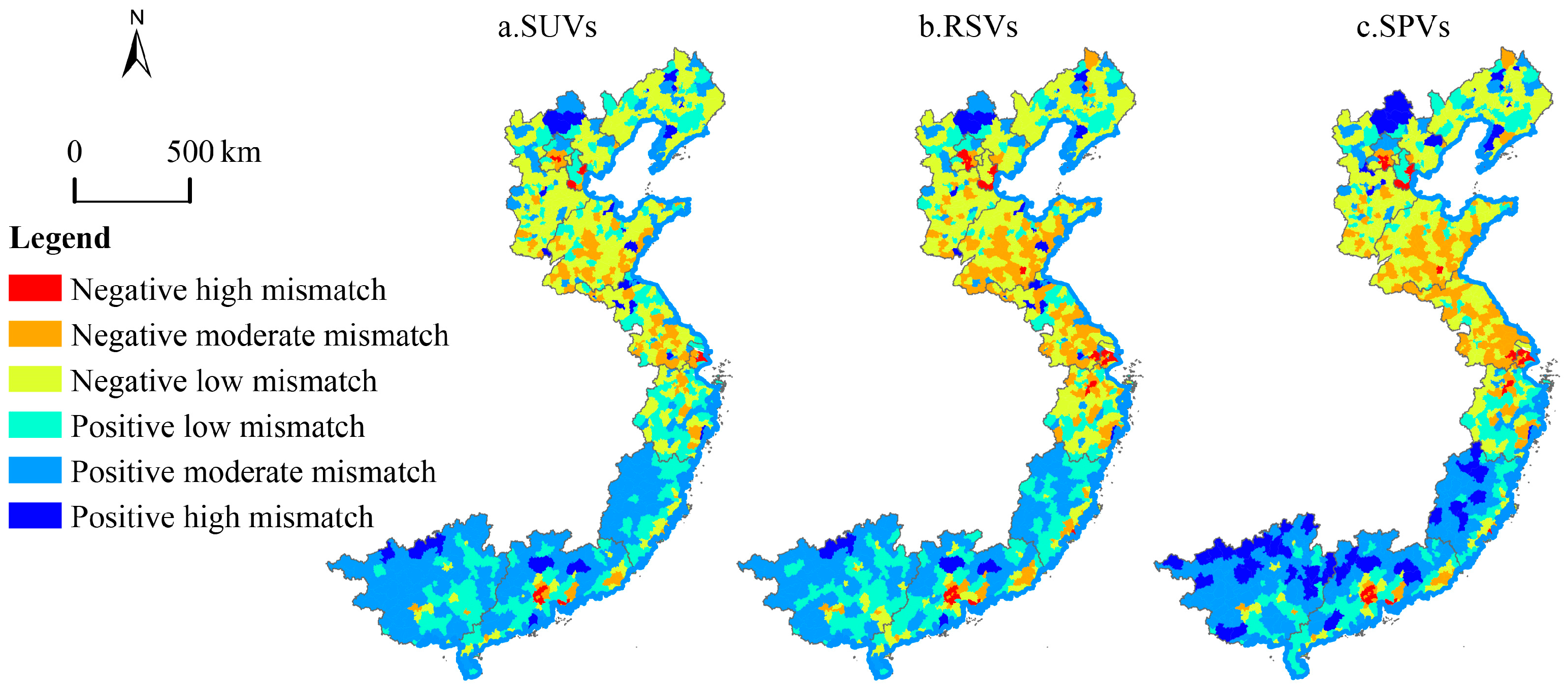
With changes in population numbers, the values of various types of ecosystem services, such as food production, gas regulation, and biodiversity conservation, also vary. To further elucidate the relationships between the ESV and population, a coordination analysis between supply services (SUVs), regulating services (RSVs), and supporting services (SPVs) with the population in 2020 was conducted. In China’s coastal areas, the coordination of supply services, regulating services, and population is similar to that of the ESV; areas with high population density generally have poorer supply and regulating services (Figure 12).

Compared with the SUVs and RSVs, the SPVs show some differences in terms of coordination (Figure 12c), with a greater number of districts exhibiting mismatches. The number of districts with SPV mismatches reached 498, accounting for 45.94% of the total research area. Among these, 285 districts were categorized as negative mismatches and 203 were categorized as positive mismatches. The numbers of mismatched districts for the SUVs and RSVs were 430 and 416, respectively. Notably, regardless of the type of service, the proportion of negatively mismatched districts is relatively high; districts where ecosystem services lag significantly behind population demands (negative high-mismatch areas) are distributed in regions with relatively high population densities (e.g., Beijing, Tianjin, Shanghai, Guangzhou, and Shenzhen). Additionally, in the southeastern hilly areas of China’s coastal areas (such as inland Fujian), SPVs exceed SUVs and RSVs. This region is characterized by a landscape of hills with predominant forested or grassland areas and relatively few cultivated lands.

4. Discussion

Ecosystems provide humans with essential services that contribute directly to the well-being of the population, such as supply, regulation, and support. The rapid expansion of built-up land due to urbanization in China’s coastal areas has led to environmental degradation, which in turn affects the well-being of the population by intensifying conflicts between humans and nature (sea) and threatening ecological security. Between 2000 and 2020, the ESV in China’s coastal areas gradually increased, indicating some improvements in ecosystem services that benefit the well-being of the population. However, owing to the increasing population and expansion of built-up land, the per capita ESV has decreased. With the continuous extrapolation of urban boundaries and the increasing intensity of construction, development, and utilization, natural surfaces such as forests, grasslands, and farmlands have been eroded, resulting in a serious loss of ecological functions, loss of biodiversity, and habitat fragmentation [47]. In coastal areas, hydrological regulation is crucial for the ESV and thus for the well-being of the population; the development of freshwater and nearshore aquaculture has significantly altered the proportion of water areas [6,48], making hydrological regulation a critical factor for the ESV and, by extension, for the well-being of the population.

Human aggregation has a major impact on the ESV [49]. Therefore, balancing the increase in human aggregation and the ESV is a key issue for sustainable development in coastal areas. In areas with high populations and high ESVs, ecological development areas should be established on the basis of ecological protection to maximize their potential ecological value. In areas with low populations and low ESVs, the main reason for low ecological service capacity is a shortage of natural resources [50]. Therefore, ecological protection plans should be developed to invigorate local ecosystem development. For areas with balanced development, maintaining the current development trend and balancing population and ecology are crucial. For mismatched areas, human activities should be controlled, with a focus on ecological development to promote regional environmental improvement.

Compared with traditional methods, correlation analysis allows for a deeper understanding of the aggregation patterns between human activities and ecosystem services, providing a clearer understanding of the distributions of population and the ESV in coastal areas. The bivariate local Moran index more precisely reflects the correlation between ecosystem services and population at the local level [50]. This precision is crucial for developing targeted interventions that can improve the well-being of the population by optimizing the relationship between human activities and the ecosystem services upon which they depend.

An in-depth exploration of the complex interactions of ecosystem services in the spatial and temporal dimensions is not only useful for building sustainable development in coastal areas and coastal zones around the globe but also crucial for enhancing the well-being of the population. This approach is essential for enhancing human resource development and improving the equalization of public services, which directly contribute to the well-being of the population [19,45]. This study provides a scientific reference for a comprehensive examination of spatial conflicts and coordination between population and ecological elements, ecosystem protection, and integrated management in China’s coastal areas, all of which are key to ensuring the well-being of the population.

However, there are areas that need further development and improvement. First, the accuracy of the ESV is directly affected by the accuracy of land use type classification. Although the current assessment references existing studies, the rough estimation of equivalence factors leads to a need for improved result accuracy, which is important for accurately assessing the services that contribute to the well-being of the population. Second, the ecological service value provided by ecological areas within urban construction land is uniformly assigned a value of zero, which partially overlooks its actual contribution to the well-being of the population. Third, ESV statistics based on administrative divisions may lose some detail and differ from the actual value of the ecological system. Future research should focus on addressing errors in ESV calculations and exploring coordination models between population and ecology at different scales. Additionally, the coordinated relationships between ESVs and other variables, such as land use changes and climate change, warrant further investigation to more comprehensively understand the dynamic interactions between populations and ecological services. Finally, the unique cultural environment and ecosystem services in coastal areas are more susceptible to the impact of water pollution. Therefore, the link between water pollution and ecosystem services will help further deepen the discussion on the factors affecting ecosystem sustainability [51]. We suggest that future research should combine factors such as land and water bodies to more comprehensively explore the relationship between the ESV and population distribution in coastal areas, ensuring that the well-being of the population is at the forefront of ecosystem management and policy-making. By doing so, we can work towards a future where the well-being of the population is supported by sustainable ecosystem services in coastal regions.

5. Conclusions

This study explores the spatial and temporal evolution characteristics of population and ecosystem service values in China’s coastal areas in 2000, 2010, and 2020 via several methods, such as geographic concentration, spatial autocorrelation, and spatial mismatch indices. These analyses are conducted with the well-being of the population in mind, as understanding how population dynamics and ecosystem services evolve over time and space is crucial for developing strategies that enhance the well-being of the population. The results indicate the following:

(1)

Over the past two decades, the population in coastal areas has increased from 58.06632 million to 70.07265 million, with increasing population density. Generally, the population is concentrated in coastal areas, with fewer people living in districts farther from the ocean. The main population centres are the Beijing–Tianjin–Hebei Urban Agglomeration, the Yangtze River Delta Urban Agglomeration, and the Pearl River Delta Urban Agglomeration, with secondary cores around provincial capitals.

(2)

The geographic concentration of ecosystem services is lower than that of the population, indicating a “low–high–low” distribution pattern from north to south. The ecosystem service value (ESV) increased from CNY 41,974.54 billion in 2000 to CNY 20,203,431.14 billion in 2020, but the per capita ESV decreased from 7228.72 yuan/person in 2000 to 6212.33 yuan/person in 2020, showing a clear downwards trend. The low ESV geographic concentration values are concentrated in the northern part of the research area.

(3)

There is a negative correlation between the ecosystem service value and population in coastal areas, indicating a significant spatial mismatch between the two, although overall coordination is relatively good. Mismatched counties are more widespread in the North China Plain and are also found in eastern Liaoning, northern Guangxi, and northern Guangdong. Increased human activities and urbanization in the Yangtze River Delta and Pearl River Delta have led to the degradation of ecological functions.

References

1. Xie, G.D.; Zhang, C.X.; Zhang, L.M. Improvement of the evaluation method for ecosystem service value based on per unit area. J. Nat. Resour. 2015, 30, 1243–1254. [Google Scholar]
2. Daily, G.C. Nature’s Services: Societal Dependence on Natural Ecosystems; Island Press: Washington, DC, USA, 1997. [Google Scholar]
3. Ouyang, Z.Y.; Wang, X.K.; Miao, H. A primary study on Chinese terrestrial ecosystem services and their ecological-economic values. Acta Ecol. Sin. 1999, 19, 19–25. [Google Scholar]
4. Costanza, R.; dArge, R.; deGroot, R.; Farber, S.; Grasso, M.; Hannon, B.; Limburg, K.; Naeem, S.; Oneill, R.V.; Paruelo, J.; et al. The value of the world’s ecosystem services and natural capital. Nature 1997, 387, 253–260. [Google Scholar] [CrossRef]
5. Liu, Y.B.; Hou, X.Y.; Li, X.W.; Song, B.; Wang, C. Assessing and predicting changes in ecosystem service values based on land use/cover change in the Bohai Rim coastal zone. Ecol. Indic. 2020, 111, 106004. [Google Scholar] [CrossRef]
6. Tan, Z.Z.; Chen, Y.Q.; Ding, J.F.; LIU, M.D.; Wang, H.; Wang, J. Simulation of land use and assessment of ecosystem service value in the eastern coastal cities of Zhejiang Province, China. Chin. J. Appl. Ecol. 2023, 34, 2777–2787. [Google Scholar]
7. Song, W.; Deng, X.Z. Land-use/land-cover change and ecosystem service provision in China. Sci. Total Environ. 2017, 576, 705–719. [Google Scholar] [CrossRef]
8. Wu, C.X.; Feng, Y.Z.; Zhao, H.; Bao, Q. Study on ecosystem service value of the Yellow River Basin in Gansu Province based on land use change. J. Desert Res. 2022, 42, 304–316. [Google Scholar]
9. Kuriqi, A.; Pinheiro, A.N.; Sordo-Ward, A.; Garrote, L. Influence of hydrologically based environmental flow methods on flow alteration and energy production in a run-of-river hydropower plant. J. Clean. Prod. 2019, 232, 1028–1042. [Google Scholar] [CrossRef]
10. Zhang, C.X.; Xie, G.D.; Yang, Q.K.; Li, S.M. Influence of human activities on the value of ecosystem services: Case study of Zhifanggou Watershed. Resour. Sci. 2008, 30, 1910–1915. [Google Scholar]
11. Reid, W.V.; Mooney, H.A.; Cropper, A.; Capistrano, D.; Carpenter, S.R.; Chopra, K.; Dasgupta, P.; Dietz, T.; Duraiappah, A.K.; Hassan, R. Ecosystems and Human Well-Being-Synthesis: A Report of the Millennium Ecosystem Assessment; Island Press: Washington, DC, USA, 2005. [Google Scholar]
12. Vitousek, P.M.; Mooney, H.A.; Lubchenco, J.; Melillo, J.M. Human Domination of earth’s ecosystems. Science 1997, 277, 494–499. [Google Scholar] [CrossRef]
13. Lu, D.D. Geographical conditions and national strategies. Adv. Earth Sci. 2020, 35, 221–230. [Google Scholar]
14. Cohen, B. Urbanization in developing countries: Current trends, future projections, and key challenges for sustainability. Technol. Soc. 2006, 28, 63–80. [Google Scholar] [CrossRef]
15. Halpern, B.S.; Walbridge, S.; Selkoe, K.A.; Kappel, C.V.; Micheli, F.; D’Agrosa, C.; Bruno, J.F.; Casey, K.S.; Ebert, C.; Fox, H.E.; et al. A global map of human impact on marine ecosystems. Science 2008, 319, 948–952. [Google Scholar] [CrossRef]
16. Dittman, D.E.; Chalupnicki, M.A.; Johnson, J.H.; Snyder, J. Reintroduction of Lake Sturgeon into the St. Regis River, NY: Post-release assessment of habitat use and growth. Northeast. Nat. 2015, 22, 704–716. [Google Scholar] [CrossRef]
17. Danz, N.P.; Niemi, G.J.; Regal, R.R.; Hollenhorst, T.; Johnson, L.B.; Hanowski, J.M.; Axler, R.P.; Ciborowski, J.J.H.; Hrabik, T.; Brady, V.J.; et al. Integrated measures of anthropogenic stress in the U.S. Great Lakes Basin. Environ. Manag. 2007, 39, 631–647. [Google Scholar] [CrossRef]
18. Robards, M.D.; Schoon, M.L.; Meek, C.L.; Engle, N.L. The importance of social drivers in the resilient provision of ecosystem services. Glob. Environ. Chang. 2011, 21, 522–529. [Google Scholar] [CrossRef]
19. Zhang, R.; Hu, C.; Sun, Y. Decoding the characteristics of ecosystem services and the scale effect in the Middle Reaches of the Yangtze River Urban Agglomeration: Insights for planning and management. Sustainability 2024, 16, 7952. [Google Scholar] [CrossRef]
20. Ba, Z.; Du, H.; Zhao, Y. Coupled and coordinated relationship between land-use cover change and ecosystem services value in horqin sandy land. Sustainability 2024, 16, 6184. [Google Scholar] [CrossRef]
21. Ma, Y.; Ling, X.; Tong, Y. Ecosystem service value estimation and spatiotemporal differentiation characteristics of typical tourism cities at grid scale: A case of Sanya. Acta Ecol. Sin. 2021, 41, 7542–7554. [Google Scholar]
22. Liang, F.C.; Liu, L.M. Quantitative analysis of human disturbance intensity of landscape patterns and preliminary optimization of ecological function regions: A case of Minqing County in Fujian Province. Resour. Sci. 2011, 33, 1138–1144. [Google Scholar]
23. Li, Y.M.; Duan, Y.P.; Jiang, D.M.; Xie, Y. Study on landscape pattern of land use and ecosystem service value under human activities in Lanping County. Res. Soil Water Conserv. 2019, 26, 293–300. [Google Scholar]
24. Menzel, S.; Kappel, C.V.; Broitman, B.R.; Micheli, F.; Rosenberg, A.A. Linking human activity and ecosystem condition to inform marine ecosystem based management. Aquat. Conserv. Mar. Freshw. Ecosyst. 2013, 23, 506–514. [Google Scholar] [CrossRef]
25. Chapin, F.S.; Carpenter, S.R.; Kofinas, G.P.; Folke, C.; Abel, N.; Clark, W.C.; Olsson, P.; Smith, D.M.S.; Walker, B.; Young, O.R.; et al. Ecosystem stewardship: Sustainability strategies for a rapidly changing planet. Trends Ecol. Evol. 2010, 25, 241–249. [Google Scholar] [CrossRef] [PubMed]
26. Li, J.; Zhou, Z.X. Natural and human impacts on ecosystem services in Guanzhong-Tianshui economic region of China. Environ. Sci. Pollut. Res. 2016, 23, 6803–6815. [Google Scholar] [CrossRef]
27. Meacham, M.; Queiroz, C.; Norström, A.V.; Peterson, G.D. Social-ecological drivers of multiple ecosystem services: What variables explain patterns of ecosystem services across the Norrstrom drainage basin? Ecol. Soc. 2016, 21, 14–39. [Google Scholar] [CrossRef]
28. Padilla, F.M.; Vidal, B.; Sánchez, J.; Pugnaire, F.I. Land-use changes and carbon sequestration through the twentieth century in a Mediterranean mountain ecosystem: Implications for land management. J. Environ. Manag. 2010, 91, 2688–2695. [Google Scholar] [CrossRef]
29. Ouyang, Z.; Zheng, H.; Xiao, Y.; Polasky, S.; Liu, J.; Xu, W.; Wang, Q.; Zhang, L.; Xiao, Y.; Rao, E.; et al. Improvements in ecosystem services from investments in natural capital. Science 2016, 352, 1455–1459. [Google Scholar] [CrossRef]
30. Chen, W.X.; Liu, Z.L.; Li, J.F.; Ran, D.; Zeng, J. Mapping the spatial relationship between ecosystem services and urbanization in the middle reaches of the Yangtze River Urban Agglomerations. Acta Ecol. Sin. 2020, 40, 5137–5150. [Google Scholar]
31. Shi, J.R.; Li, S.X.; Song, Y.; Zhou, N.; Guo, K.L.; Bai, J. How socioeconomic factors affect ecosystem service value: Evidence from China. Ecol. Indic. 2022, 145, 109589–109600. [Google Scholar] [CrossRef]
32. Baima, Z.G.; Xiao, Y.; Ouyang, Z.Y.; Wang, L.Y. Assessment of ecological conservation effect in Xishui county based on gross ecosystem product. Acta Ecol. Sin. 2020, 40, 499–509. [Google Scholar]
33. Zhang, Z.P.; Xia, F.Q.; Yang, D.G.; Huo, J.W.; Wang, G.L.; Chen, H.X. Spatiotemporal characteristics in ecosystem service value and its interaction with human activities in Xinjiang, China. Ecol. Indic. 2020, 110, 105826–105837. [Google Scholar] [CrossRef]
34. Ouyang, X.; Zhu, X.; He, Q.Y. Spatial interaction between urbanisation and ecosystem services: A case study in Changsha-Zhuzhou-Xiangtan urban agglomeration, China. Acta Ecol. Sin. 2019, 39, 7502–7513. [Google Scholar]
35. Zhu, X.J.; Xue, L. Changes of ecological service value and its coupling with economic development in Guanzhong region. Chin. J. Ecol. 2022, 41, 769–776. [Google Scholar]
36. Gao, X.; Shen, J.Q.; He, W.J.; Zhao, X.; Li, Z.C.; Hu, W.F.; Wang, J.Z.; Ren, Y.J.; Zhang, X. Spatial-temporal analysis of ecosystem services value and research on ecological compensation in Taihu Lake Basin of Jiangsu Province in China from 2005 to 2018. J. Clean. Prod. 2021, 317, 128241–128259. [Google Scholar] [CrossRef]
37. Xie, G.D.; Zhen, L.; Lu, C.X.; Xiao, Y. Expert knowledge based valuation method of ecosystem services in China. J. Nat. Resour. 2008, 23, 911–919. [Google Scholar]
38. Xu, L.F.; Xu, X.G.; Luo, T.; Zhu, G.R.; Ma, Z.W. Services based on land use: A case study of Bohai Rim. Geogr. Res. 2012, 31, 1775–1784. [Google Scholar]
39. Xie, G.D.; Zhang, C.X.; Zhen, L.; Zhang, L.M. Dynamic changes in the value of China’s ecosystem services. Ecosyst. Serv. 2017, 26, 146–154. [Google Scholar] [CrossRef]
40. Wang, L.; Duan, X.J.; Tian, F.; Qin, X.H. Study on the relationship between population and economic spatial distribution in Yangtze River Delta. Econ. Geogr. 2009, 29, 1619–1623. [Google Scholar]
41. Deng, Y.; Liu, S.H.; Cai, J.M.; Lu, X. Spatial pattern and its evolution of Chinese provincial population and empirical study. J. Geogr. Sci. 2014, 69, 1473–1486. [Google Scholar] [CrossRef]
42. Zhu, Y.X.; Zhang, J.Z. Trend surface analysis of population density of Gansu based on gis and surfer. Comput. Syst. Appl. 2008, 12, 65–68+53. [Google Scholar]
43. Anselin, L. Under the hood-Issues in the specification and interpretation of spatial regression models. Agric. Econ. 2002, 27, 247–267. [Google Scholar] [CrossRef]
44. Sridharan, S.; Tunstall, H.; Lawder, R.; Mitchell, R. An exploratory spatial data analysis approach to understanding the relationship between deprivation and mortality in Scotland. Soc. Sci. Med. 2007, 65, 1952–1963. [Google Scholar] [CrossRef] [PubMed]
45. Kong, X.M.; Lu, L.; Ren, Y.S.; Jiang, W.F.; Li, D.H. Study on the spatial-temporal evolution characteristics and coordination of population and ecosystem services value in central China. Resour. Dev. Mark. 2024, 40, 205–216. [Google Scholar]
46. Zeng, Y.M. Simulation and projection on the pattern of Chinese population spatial distribution: Research with population density of county level based on the 5~(th) and 6~(th) population census of China. Popul. Econ. 2016, 6, 48–61. [Google Scholar]
47. Luo, Z.; Yang, X.; Luo, S. Land use simulation and ecological network construction around Poyang Lake Area in China under the goal of sustainable development. Sustainability 2024, 16, 8146. [Google Scholar] [CrossRef]
48. Yao, Y.Z.; Song, Y.T.; Xue, Y.T.; Jia, C.G.; Wang, Z.C.; Zhang, G.H. Spatial-temporal variations and mechanism of ecosystem services value from land use perspective: A case study of Liaoning coastal zones. Areal Res. Dev. 2024, 43, 153–159. [Google Scholar]
49. Kuzyshyn, A. Spatial diversification of the social sphere development in the Carpathian-Podillia Region. Folia Geogr. 2019, 61, 144–162. [Google Scholar]
50. Ai, M.S.; Chen, X.; Yu, Q. Spatial correlation analysis between human disturbance intensity (HDI) and ecosystem services value (ESV) in the Chengdu-Chongqing urban agglomeration. Ecol. Indic. 2024, 158, 111555–111563. [Google Scholar] [CrossRef]
51. Utkina, K.; Kresin, V.; Brook, V.; Lisnyak, A. Integrated criteria for ranking Black Sea land-based point pollution sources. Folia Geogr. 2017, 59, 35–49. [Google Scholar]
Figure 1. Overview of China’s coastal areas.
Sustainability 16 10212 g001
Figure 2. Spatial distribution of population density in 2000, 2010, and 2020.
Sustainability 16 10212 g002
Figure 3. Spatial distribution of population geographic concentration in 2000, 2010, and 2020.
Sustainability 16 10212 g003
Figure 4. Trend analysis of population density in 2000, 2010, and 2020. Black represents the trend surface data distributed according to geographic space, green represents the distribution projected according to longitude, and blue represents the distribution projected according to latitude.
Sustainability 16 10212 g004
Figure 5. Kernel density analysis of population in 2000, 2010, and 2020.
Sustainability 16 10212 g005
Figure 6. Spatial distribution of per capita ecosystem service values in 2000, 2010, and 2020.
Sustainability 16 10212 g006
Figure 7. Spatial distribution of eco-geographic concentrations in 2000, 2010, and 2020.
Sustainability 16 10212 g007
Figure 8. Trend analysis of per capita ecosystem service values in 2000, 2010, and 2020. Black represents the trend surface data distributed according to geographic space, green represents the distribution projected according to longitude, and blue represents the distribution projected according to latitude.
Sustainability 16 10212 g008
Figure 9. Kernel density analysis of per capita ESVs in 2000, 2010, and 2020.
Sustainability 16 10212 g009
Figure 10. Local spatial autocorrelation of bivariate population geographic concentration and ecological geographic concentration in 2000, 2010, and 2020.
Sustainability 16 10212 g010
Figure 11. Spatial and temporal patterns of spatial dislocation of population and ecosystem service values in 2000, 2010, and 2020.
Sustainability 16 10212 g011
Figure 12. Coordination of coastal area populations with supply services (a), regulating services (b), and supporting services (c).
Sustainability 16 10212 g012