Abstract
This study aims to contribute to the reduction of carbon dioxide and the production of hydrogen through an investigation of the photocatalytic reaction process. Machine learning algorithms can be used to predict the hydrogen yield in the photocatalytic carbon dioxide reduction process. Although regression-based approaches provide good results, the accuracy achieved with classification algorithms is not very high. In this context, this study presents a new method, Adaptive Neural Architecture Search (NAS) using metaheuristics, to improve the capacity of ANNs in estimating the hydrogen yield in the photocatalytic carbon dioxide reduction process through classification. The NAS process was carried out with a tool named HyperNetExplorer, which was developed with the aim of finding the ANN architecture providing the best prediction accuracy through changing ANN hyperparameters, such as the number of layers, number of neurons in each layer, and the activation functions of each layer. The nature of the NAS process in this study was adaptive, since the process was accomplished through optimization algorithms. The ANNs discovered with HyperNetExplorer demonstrated significantly higher prediction performance than the classical ML algorithms. The results indicated that the NAS helped to achieve better performance in the estimation of the hydrogen yield in the photocatalytic carbon dioxide reduction process.
1. Introduction
Today, a large proportion of energy is produced using fossil fuels. This results in high carbon emissions and environmental pollution. The high level of carbon dioxide (CO2) in the atmosphere is one of the main causes of global warming. There is an urgent need to reduce dependence on fossil fuels and focus on renewable energy. In this context, hydrogen is considered to be a clean and renewable substance that can act as a perfect energy carrier. Photocatalysis is a technique that utilizes sunlight to aid chemical reactions, such as the conversion of CO2 into renewable substances such as hydrogen. The technique aids in reducing the carbon levels in the atmosphere, while increasing the production of clean energy carriers, such as hydrogen. Hydrogen production through the photocatalytic reduction of CO2 is an active research field. In a photocatalytic CO2 reduction process, the amount of outputs (such as hydrogen yield) can be estimated using predictive methods, such as Machine Learning (ML). Although several machine learning methods have been implemented and tested for hydrogen production (such as in [1], Ren et al. [2], Mageed [3], Ramkumar et al. [4], and Yurova et al. [5]) and significantly good results were achieved using the regression-based approach, the predictive ability of these methods has remained limited in studies conducted with classification methods. On the other hand, artificial neural networks have very flexible architecture, which provides options for improvement. In this study, we explore whether ANN architectures, which provide high classification accuracy in the prediction of gas (hydrogen) yield as a result of photocatalytic CO2 reduction process, can be discovered through an adaptive Neural Architecture Search (NAS). Experiments were conducted in our study in parallel with this aim, and the results of the experiments demonstrated that ANN architectures with significantly higher prediction performance than those of the classical ML algorithms can be discovered. The implementation of these newly discovered architectures in practice will aid in classifying the (hydrogen) yield as a result of the photocatalytic CO2 reduction process with a high accuracy. The following section presents our findings on the literature review; this paper continues with a section on the methodology and concludes after the presentation of results and discussion.
Literature Review
Increasing amounts of production with industrial development cause rapid consumption of natural resources, while causing increased carbon emissions, environmental pollution, and the destruction of nature by production-oriented industries [6]. With the rapid increase in the world’s population, the energy demands of societies have grown exponentially, and the per capita energy consumption rate and the atmospheric CO2 level have reached alarming levels. Today, about 85% of energy needs are met by fossil fuels, including oil, coal, and natural gas [7]. If energy consumption continues in this way, it is predicted that a serious energy crisis will be faced soon. To prevent this crisis, it is necessary to reduce dependence on fossil fuels [8]. Intense carbon emissions cause an increase in greenhouse gas emissions in the atmosphere, leading to global warming and adverse changes that pose a threat to ecosystems [9]. Production based on fossil resources is not sustainable and negatively affects independence [10]. The use of nonrenewable energy sources, which are used to meet energy needs, causes irreparable harm to the environment. As a result of the use of these energy sources, many negative consequences, such as air pollution, water pollution, global warming, and acid rains, occur. Furthermore, the reserves of these resources are limited. For this reason, it has become an inevitable necessity to develop renewable energy sources that are less harmful to the environment and techniques for obtaining energy from these sources. Energy is considered one of the most important indicators of development. In this changing and developing world, the importance of energy is increasing day by day. Energy resources are rapidly depleting, energy costs are increasing, and environmental awareness is developing in societies. To meet energy demand and protect the environment, developing and developed countries are moving to renewable energy sources [11]. Renewable energy resources, which represented 7.7% of total energy consumption in the world in 2005, are expected to increase to 8.5% in 2030 [12]. Among these energy sources, hydrogen energy, which is environmentally friendly and abundant in nature, has come to the fore. Table 1 shows the global atmospheric CO2 concentration.

Table 1.
Average monthly global atmospheric CO2 concentration measured in parts per million (ppm) [13].
As shown in Table 1, CO2 emissions increase year by year. Greenhouse gas emissions, i.e., CO2 emissions caused by the use of fossil fuels, trigger risks of climate change [14]. According to the scenarios of the Intergovernmental Panel on Climate Change (IPCC), the rates of greenhouse gases, such as carbon dioxide and methane, in the world’s atmosphere have increased in parallel with human activities and social–economic development since the industrial revolution. Global warming will exceed the 1.5 °C limit between 2030 and 2052 if greenhouse gas emissions continue [10]. This clearly shows that it is necessary to change the current approaches to energy production and consumption. For this reason, hydrogen production through CO2 reduction is an issue that should be taken seriously.
Hydrogen contains high energy and carries energy, is clean, renewable, and convertible to other forms of energy, and since it can be stored, it reduces the problem of energy storage [15,16]. The main energy sources in nature are primary energy sources. Secondary energy sources obtained by converting primary sources to different physical states are called energy carriers [17]. The fact that hydrogen carries energy indicates that it can be produced using primary energy sources [18]. Hydrogen is the main component of water that covers 60% of our planet. Hydrogen exists in different forms in living things and fossil fuels [15]. Hydrogen gas was produced by Henry Cavendish in 1766. Seventy-three years later, in 1839, William Robert Grove developed fuel cells using hydrogen [19]. Components in which hydrogen is used as a fuel and chemical energy is directly converted into electrical energy are called fuel cells [20]. The production process and the use of hydrogen are emission-free. Commercial hydrogen production is carried out with a high percentage of fossil materials. When we look at the world’s hydrogen production at the end of 2021, it can be seen that 48% is from natural gas, 30% is from refinery products, 18% is from coal, and 4% is from water [21].
Although water consists of two hydrogens and one oxygen, fossil fuels are composed of hydrogen and carbon. The greatest difficulty in obtaining hydrogen is its separation from other compounds [22].
On a global scale, although there are concerns about energy consumption, energy is actually transformed, rather than consumed. What has changed is the raw energy materials, which are formed in certain geological periods and are produced and consumed in different ways and used in energy production [23].
The increase in the processing power of computers has led to the emergence of concepts such as optimization, machine learning, and artificial intelligence. Hydrogen energy and photocatalytic CO2 reactions with big data have become very suitable topics for optimization and machine learning. Machine learning is used in many different fields, such as civil engineering [24,25,26,27,28,29,30], machine vision [31], optics [32], and biomedicine [33]. There are many studies that have used optimization and artificial intelligence in hydrogen energy and photocatalytic CO2 reactions.
Ren et al. [2] developed a model for photocatalysis to produce maximum hydrogen and used Gaussian Process Regression (GPR) to find the optimal parameters. In order to increase the success of the model, Whale Optimization (WO) and Simulated Annealing (SA) algorithms were applied, and successful results were obtained. Saadetnejad et al. [1] applied Random Forest to predict the band gap while investigating the gas phase of photocatalytic CO2 reduction for hydrogen production and obtained low error values. The Decision Tree applied for total hydrogen production also showed 80% success for the gas phase. Mageed [3] utilized two different ANNs, the Support Vector Machine (SVM), the Nonlinear Regression Model (NLM), and the Response Surface Model (RSM) to model hydrogen production. According to the results, ANN had a better prediction rate (R = 0.998), compared with the other models. Yan et al. [34] associated g-C3N4 and the hydrogen production rate using machine learning and demonstrated the success of the ML models. Xu et al. [35] used machine learning to explore alternative copolymers. Haq et al. [36] used different machine learning models and the Genetic Algorithm (GA) to predict the hydrogen yield for supercritical water gasification. Based on the results obtained, this ML-based method achieved an accurate estimate of hydrogen yield (R2 = 0.997). Ramkumar et al. [4] predicted the hydrogen production value by photolysis using ANN. As a result of their study, they reached an accuracy value of 91.66%. Yurova et al. [5] used the ML models Gradient Boosting, Multilayer Perceptron, and Random Forest to predict the efficiency of photocatalytic hydrogen production. The models showed high prediction success with R2 values greater than 0.9.
In recent years, photocatalytic technology has started to become an emerging topic to tackle environmental pollution [37]. To understand photocatalytic systems, it is necessary to mention the concept of photocatalysis. Photocatalysis is a combination of the words photo and catalysis, which means accelerating a chemical reaction. In other words, photocatalysis is the acceleration of a chemical reaction (photoreaction) that occurs under the influence of light (UV rays or sunlight) in the presence of a catalyst [38]. The photocatalysis method is economical, highly efficient, practical, and easy to implement [39]. On the basis of this phenomenon, photocatalytic systems have been developed. Photocatalysis is a photocatalytic technique [40]. The photocatalysts used generally show activity under ultraviolet (UV) irradiation, and various strategies have been developed to reduce the bandwidth, as the high bandwidth makes them not active enough under the visible region or sunlight. Among these, techniques such as the addition of different metal or nonmetal additives, surface modification, formation of composites with another semiconductor, and modification with carbon-based materials are preferred [41]. With the photocatalytic technique, pollutants can be completely broken down. The removal of the catalyst from the reaction medium and poor chemical stability caused by the large surface area are serious problems that can occur. Better photocatalytic activity is obtained when a semiconductor with lower band-gap energy is selected [42]. Figure 1 represents the proposed mechanism for a photocatalytic reaction.

Figure 1.
Mechanism of a photocatalytic reaction on a semiconductor photocatalyst [43].
The dataset used in this study is related to the photocatalysis process. Many semiconductors, such as TiO2, rG, SiC, GO, lnTaO4, Ta2O5, CeO2, ZrO2, CaFe2O4, BaLa4Ti4O15, CdS, ZnO, ZnTe, C3N4, TiO2BP, Zn2Ti3O8, PbBiO2Br, CeO2, Fe2O3, SrTiO3, ZnS, SrNb2O6, TaON, BiVO4, and ZnGa2O4, were the photocatalysts in the dataset (which will be explained in detail in the following section). One of the most used semiconductors in the dataset was TiO2. TiO2 has an appropriate band gap energy, high photocatalytic activity, is chemically and biologically inert, low-cost, mechanically durable, and non-toxic [44]. TiO2 is a widely used semiconductor in many scientific studies [45,46].
2. Materials and Methods
2.1. The Dataset
In this study, the dataset provided by Saadetnejad et al. [1] was used for model evaluation. This dataset consisted of 549 data points. In the compilation of the dataset, the data were collected from 80 studies that focused on the photocatalysis (photocatalytic CO2 reduction) process. The aim of this process was to produce hydrogen. The dependent variable in the dataset, namely total gas yield, indicated hydrogen yield as a result of photocatalysis. The aim of our study was to facilitate and improve the estimation and classification of the total gas yield (hydrogen production) of the photocatalysis process through a neural architecture search. Details of the dataset and the collected references to the data can be found in [1] for further exploration. At the beginning of our study, the source dataset [1] was divided into two datasets according to the gas and liquid phases of the photocatalysis process. The number of rows was 549 in the source dataset; after the separation of the source dataset into two new datasets, the gas phase dataset contained 268 records and the liquid phase dataset contained 281 records. The metadata of these two datasets (before the data preprocessing stage) are provided in Table 2 for the (new) gas-phase dataset and Table 3 for the (new) liquid-phase dataset.
Table 2.
Gas-phase dataset.
Table 3.
Liquid-phase dataset.
For both datasets, the dependent variable bins were chosen within the same ranges given in [1], and 3 classes were defined as A, B, and C to denote these bins. With this approach, the dependent variable (total gas yield) was transformed into a categorical variable instead of a continuous one. The ranges of values for each class of the dependent variable are given in Table 4 and Table 5.
Table 4.
Range and instance numbers of classes A to C for the dependent variable for the gas dataset.
Table 5.
Range and instance numbers of classes A to C for the dependent variable for the liquid dataset.
2.2. Data Preprocessing
Real-world data from different sources can be noisy, inconsistent, and incomplete. Therefore, raw data need to be converted to a suitable format for analysis. In this step, the data are prepared for the analysis phase by cleaning, merging, transformation, and reduction. Operations such as data cleaning, data transformation, and data reduction used in data preprocessing may affect the success of the ML model. This step in ML is called data preprocessing and includes all actions taken before modeling [47]. As not applying preprocessing can cause unsuccessful results, it is important to increase data quality and prepare for data mining by preprocessing the data to obtain high accuracy and reliability [48]. The data preprocessing methods (data transformation and missing value imputation) used in this study are shown in Figure 2.

Figure 2.
Data preprocessing methods (edited from [49]).
For the data preprocessing stage and for training the ML models (in the last stage) of this study, Python 3.10.11 [50] Anaconda3 [51] environment, Spyder 5.2.2. [52] interface, NumPy [53] and Pandas [54] libraries, and Scikit-Learn [55] libraries are used.
2.2.1. Data Transformation
Since machine learning algorithms do not work directly on categorical data (in the form of string), the data must be converted into numerical data. In this study, One Hot Encoding was used to convert categorical values into numerical values. Categorical data (non-numeric) are not used directly in machine learning algorithms. Before the data can be used, they must be expressed in numerical form. The One Hot Encoding (OHE) method is generally used for the numerical encoding of categorical data [56]. Each integer value is represented as a binary vector with all zero values except for the integer index marked with 1, as shown in Figure 3.

Figure 3.
One hot encoding example [57].
For the variables with the numerical data, Standard Scaler of the Scikit-Learn [55] was used to scale the variables.
2.2.2. Data Imputation
The reason for the missing values in the data set is that people do not share the information during observation, the relevant information is not entered when collecting the data, and there are systemic errors or data losses [58]. The Scikit-learn machine learning library of Python includes the SimpleImputer [55] class, which supports imputation by taking the most frequent or mean values of the variable (column).
We observed missing values in two fields of the dataset, which were “Band Gap Energy” for the gas- and liquid-phase datasets and “Feed Molar Ratio” for the gas-phase dataset. The data of both these fields were numerical. Due to two reasons, (i) the missing values of this variable being predicted using the other fields of the dataset [1] (i.e., the type of variable cannot be considered as a fully independent variable after this), and (ii) there being a high ratio of synthetically generated data (i.e., 1/3) [1], we chose to exclude this field from our input dataset. For the “Feed Molar Ratio” field, where the missing data ratio is 12.3%, it is advised by the literature that the data with a missing ratio of over 10% should be imputed; in addition, the data with a missing ratio between 5% and 10% can be considered or evaluated for imputation [59,60]. We wrote software code (available upon request) to test if the missing data followed the MAR, MCAR, or MNAR pattern, and we observed that the data followed a MCAR pattern; we chose to use the mean imputation for this field. In the Scikit-Learn SimpleImputer class, the default imputation strategy is mean if the values of a field are numerical, and this strategy is implemented for the “Feed Molar Ratio” field.
At the end of this method, all features in the data set were converted to numerical features. Table 6 presents all input variables and their sizes.
Table 6.
Sizes of one hot encoded input variables.
Following the data preprocessing stage, the size of the gas-phase dataset was 67 and the size of the liquid-phase dataset was 90. In the next stage, a new tool developed by the authors was utilized to discover the most accurate ANN architecture for the prediction of the total gas yield in a photocatalytic CO2 reduction process.
2.3. Adaptive NAS and HyperNetExplorer
Neural Architecture Search (NAS) has emerged as a subfield of automated machine learning (AutoML) for discovering the most accurate ANN architecture by searching architectural hyperparameters, such as the number of layers, number of neurons, and activation functions. The search can be conducted with traditional methods, such as grid search or random search, or adaptive methods (i.e., methods that adjust search based on ongoing results), such as optimization algorithms. In this research, we first utilized HyperNetExplorer, developed by our research group. HyperNetExplorer is a web-based NAS tool that aims to find an ANN architecture that provides the most accurate classification/regression (ML) model for a given dataset. This section will detail how HyperNetExplorer was developed and operated. HyperNetExplorer depends on ANNs and uses several optimization algorithms from the MealPy [61] package for hyperparameter optimization. The following sections provide information on ANN architectures, hyperparameter optimization algorithms, validation, and performance evaluation strategies, and finally elaborate on the HyperNetExplorer architecture.
2.3.1. Artificial Neural Networks (ANNs)
Artificial neural networks are computational networks that try to completely mimic the nerve cell networks of the nervous system and take samples from the human brain [62]. Artificial neural networks, like humans, gain experiences, store them in memory, and use their experiences. Artificial neural networks started with detailed studies of the human brain by scientists in the late 1800s. The artificial neural network model was first introduced in 1943 by Warren McCulloch and Walter Pitts [63]. Artificial neural networks can work only with numerical information. The symbolic expressions used must be converted into numerical values [64]. The smallest units that form the basis of an ANN’s work are called artificial neural cells or processing elements. Figure 4 shows the simplest artificial neural cells of 5 main components: inputs, weights, sum function, activation function, and output.
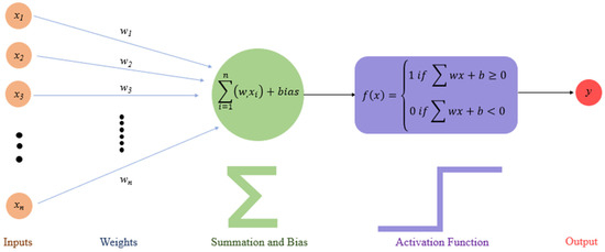
Figure 4.
Structure of artificial neural networks [65].
Inputs (x1, x2, x3, … xn) are information entering the cell from other cells or external environments. These are determined by the examples the network is asked to learn. Weights (w1, w2, w3, … wn) are values that express the effect of an input set or another processing element in a previous layer on this processing element. Each input is aggregated through the sum function, multiplied by the weight that connects that input to the processing element [66]. Since artificial neural networks are required to learn non-linear states, the activation function is applied to the outputs of artificial nerve cells. Artificial neural networks work against nonlinear results when the output of artificial nerve cells is active [67]. Activation functions provide coupling between input and output units. When the activation function is selected correctly, network performance is severely affected [68]. Figure 5 shows activation function graphs.
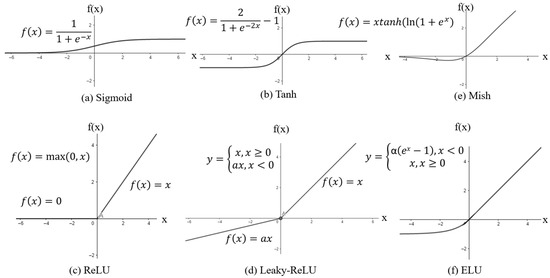
Figure 5.
Activation functions.
Sigmoid/LogSigmoid Activation Function: The sigmoid activation function, which is frequently used in classification problems, transforms incoming inputs into outputs by generating between 0 and 1, as shown in Figure 5a [69]. The logistic sigmoid function (logSigmoid) is a type of sigmoid function, which produces outputs on scale (−∞, 0).
Tangent hyperbolic activation function (TanH): The tangent hyperbolic activation function is very similar to the sigmoid function, but the output range of the function is between −1 and +1. As can be seen in Figure 5b, the outputs with values in the [−1, 1] range are zero-centered, thus facilitating optimization, and this function is preferred more often than the sigmoid activation function [69].
Rectified Linear Unit Function (ReLU): The ReLU activation function converts the incoming inputs into outputs between 0 and +∞, as shown in Figure 5c. Therefore, it is called a rectified linear function and can be quickly calculated [69].
Leaky Rectified Linear Unit Function (Leaky ReLU): Since ReLU directly equates negative values to zero (Figure 5c), the units in the layers do not become active in cases where there are many negative values. To avoid this situation, the Leaky-ReLU activation function was proposed. As shown in Figure 5d, in order to add slope to the function at negative values, a small constant value, such as 0.01, is chosen for the leakage value in the Leaky-ReLU method [69].
Mish Activation Function: The Mish activation function (Figure 5e) presents a new and nonmonotonic approach to other functions. It performs well with the standard activation function [70].
Exponential Linear Unit (ELU): The exponential linear unit (Figure 5f) is similar to ReLU, except for the negative inputs. For negative input, the alpha parameter is usually taken [71].
2.3.2. Algorithms for Hyperparameter Optimization
In this study, different optimization algorithms were used for ANN hyperparameter optimization. These algorithms were the Flower Pollination Algorithm (FPA), Genetic Algorithm (GA), Harmony Search (HS), Jaya Algorithm (JA), Particle Swarm Optimization (PSO), and Teaching–Learning-Based Optimization Algorithm (TLBO). Information about these algorithms is given below. A comparison table for the algorithms is given in Table 7.
Flower Pollination Algorithm (FPA): FPA is an algorithm inspired by the flower reproduction process and can mimic pollination in plants to achieve the best result in the shortest time for solving global optimization problems. The main goal of flower pollination is to ensure optimal vigor and an optimal biological reproduction stage. Pollination and other factors interact optimally to reproduce plants [72].
Genetic Algorithm (GA): GA is a search and optimization algorithm in which evolutionary processes are imitated [73]. The genetic algorithm achieves the best results in the search space due to selection, crossover, and mutation, as in evolutionary processes [74].
Harmony Search (HS): The HS algorithm is a music-based algorithm and mimics the path musicians take to find the most compatible harmony. The fitness value is determined by assigning initial values to the solution parameters of the investigated problem. Good results are retained in the harmony memory, while the worst results are removed from the memory. This process continues until the best one is found [75].
Jaya Algorithm (JA): JA is an algorithm named Jaya, a Sanskrit word that means victory, because it tries to achieve victory by reaching the best solution [76]. The algorithm constantly tries to approach good solutions to achieve success and to stay away from bad solutions to avoid failure.
Particle Swarm Optimization (PSO): Particle Swarm Optimization (PSO) is a population-based algorithm inspired by the swarm behavior of bird flocks and fish schools during foraging and/or escaping from danger. In PSO, decision variables do not need to take a special initial value to solve the problem. Since the PSO is population-based, it is possible to search for global solutions in multiple directions [77].
Teaching–Learning-Based Optimization Algorithm (TLBO): The TLBO algorithm is a population-based algorithm. The algorithm is based on the teaching–learning process. In the proposed algorithm, each candidate solution is expressed by a set of variables representing the results of a student. The process in which students try to improve their results by receiving information from the teacher is called the teacher phase. It is also the student phase in which they improve their performance by interacting with other students [78].
Table 7.
Comparison table for algorithms.
Table 7.
Comparison table for algorithms.
| Algorithm | Advantages | Disadvantages | Types of Optimization Problems Best Suited for | Convergence Rates |
|---|---|---|---|---|
| FPA | Simplicity and flexibility | Inadequate optimization precision [79] | Large integer programming problems, high-complexity convergence problems | Poor |
| GA | Parallel capabilities and flexibility | Difficult interpretation of solutions | Timetabling and scheduling problems | Slow |
| HS | No need for derivative information [80] | Stuck at the local optimum | Multi-objective optimization problems | Fast |
| JA | Simplicity, efficiency, and no algorithm-specific parameters | Get stuck in local minima | Large -scale real-life urban traffic light scheduling problems | Medium |
| PSO | Flexible and easy to implement | Easy stuck to local optimum | Constrained and unconstrained (one or more objective) optimization problems | Slow |
| TLBO | Powerful exploration | Suboptimal performance | Complex optimization problems | Fast |
The complexity of algorithms can be expressed mathematically in Big-O Notation. According to the Big-O Notation, the letter O (i.e., function’s order) indicates the asymptotic upper bound of a function’s growth rate [81]. The growth rate describes how quickly the runtime or space increases as the input size N grows. Table 8 illustrates the equations for the temporal and spatial complexity of the algorithms.
Table 8.
Complexity of algorithms (Big-O Notation).
In Table 8, T is the number of generations/iterations, N is the population/swarm size, and D is the problem dimensions. (For our case T = 50, N = 20, D = 7). The temporal complexity ranking of these algorithms is provided in Equation (1).
For hyperparameter optimization in ANNs, f(D) can be denoted as Equation (2).
In Equation (2), E is the number of epochs, B is the batch number, M is the dataset size, and W(D) is the number of total connections in the ANN (which changes in every iteration of the algorithm, based on the selected combination of hyperparameters). Given these variables, the temporal complexities of the algorithms can be re-written as Equations (3)–(8):
2.3.3. Validation and Performance Evaluation Strategies
k-Fold Cross-Validation
Cross-validation is a method used to reevaluate machine learning methods within the dataset used. The method is called k-fold cross-validation because a parameter named k is used in the method, which expresses the number of groups into which the selected data set will be divided. The selected k-value determines how many folds of cross validation in the model will be tested [88].
Since k = 10 in Figure 6, there were 10 folds. In the first round, 1 line in the yellow part is taken for testing and 9 lines are taken for training. The first round ends, so the success rate is achieved and the algorithm learns. The same process is applied to the other rounds so that all of the data enter both training and testing. As parameter k is selected as 10, the model was tested with 10-fold cross-validation.
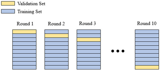
Figure 6.
k-fold cross validation [89].
Performance Evaluation
In classification problems, in order to measure the performance of the trained model, the prediction results of the model are transformed into the confusion matrix for a more explanatory analysis [90]. In a confusion matrix, as shown in Table 9, values under the name True indicate the number of predictions made correctly, and values under the name False indicate the number of predictions made incorrectly. Each column contains the actual value, and each row contains the estimated value. Thus, the cells that continue diagonally from the top left to the bottom right give the accuracy of the prediction result, and the other cells give the error rate.
Table 9.
Confusion matrix.
After the confusion matrices are generated, the classification metrics must be evaluated. For this, it is necessary to specify how much of the results from the first model are correctly predicted. For this purpose, the measurement of the accuracy rate is one of the scales used for classification methods. Accuracy is obtained by correctly dividing classified data into all data (Equation (9)) [91].
Other performance metrics, such as precision, recall, and F1 score, were calculated using TP, TN, FP and FN. Precision measures how many of the instances that the classification model predicts as positive are actually positive. A high precision value indicates that the positive predictions of the model are indeed positive. Precision is calculated by Equation (10) [85].
Recall measures how many true positives the classification model is able to detect. A high recall value indicates that the model is less likely to miss true positives. Recall is calculated by Equation (11) [92].
The F1 score is the harmonic mean of the precision and recall metrics of the classification model. With the F1 score, the performance of the model is evaluated in a single metric by combining precision and recall values in a balanced way. The F1 score value is calculated by Equation (12) [93].
2.3.4. HyperNetExplorer: Architecture and Operation
HyperNetExplorer depends on ANNs and utilizes several optimization algorithms from the MealPy [61] package for hyperparameter optimization of ANN. The tool was developed with Python and Pytorch [94] (as the ANN framework) and utilized Streamlit as the GUI [95]. The parameters to be optimized and their ranges are provided in Table 10.
Table 10.
Parameters to be optimized.
In the default configuration of the tool, the learning rate is 0.001, and the number of epochs is 200, but this can change depending on the type of the problem. In the default configuration of the tool, CrossEntropyLoss is used as the loss function for the network for classification and MSELoss is used for the network for regression-type problems. The tool can utilize all the optimization algorithms provided by the MealPy package. In the current configuration of the tool utilized for this dataset, the Flower Pollination Algorithm (FPA), Genetic Algorithm (GA), Harmony Search (HS), Jaya Algorithm (JA), Particle Swarm Optimization (PSO), and Teaching–Learning-Based Optimization Algorithm (TLBO) are used. The population size for all algorithms was 20 and number of generations was 50 for all algorithms. Further information about the algorithm implementations can be found in [61,96,97,98]. The dataset could be uploaded to the system using the GUI; following this, once the FindBestNet command is given through the GUI, the objective function of the tool generates an ANN in every iteration of the optimizer based on a set of the hyperparameters provided by the optimizer. Once an ANN is generated, the accuracy of this ANN is calculated through 10-fold cross validation and the mean accuracy of this 10-fold validation is output as the output of the objective function. This output is consumed/evaluated by the optimizer and based on this, the objective function is called again with a new set of hyperparameters. The default parameters for the optimizer (i.e., not the main tool) is 20 epochs and a population size of 50, which generates a minimum of 20 × 50 = 1000 ANN architectures in every run. The values of the parameters for each generated network and accuracies are provided as a table in the Streamlit-based GUI. Once the training is finished, all ANN models are kept on the server and can be downloaded as (*.pt) files. The ANN model with the best accuracy could then be used in a production/testing environment.
2.4. Utilisation of Conventional Machine Learning Algorithms
Within the scope of the study, to validate that the accuracies achieved by ANNs discovered by HyperNetExplorer are significantly superior to the classical (well-known) ML algorithms, in the following stage, the Decision Tree, Gaussian NB, K-Nearest Neighbors (KNN), Linear Discriminant Analysis (LDA), Support Vector Machine, Random Forest, Gradient Boosting, and Histogram Gradient Boosting classifiers from Scikit-Learn package (v 1.3.0) [55] and CatBoost classifier from the CatBoost package [99] were utilized.
The validation and performance evaluation strategy was 10-fold cross-validation, similar to the strategy chosen for the HyperNetExplorer. The mean accuracy of 10-fold cross-validation is considered as the overall accuracy of the classification. The default parameters for the ML models are given in Table 11.
Table 11.
Default parameters of the ML models used in this study.
2.4.1. Decision Tree (DT)
A decision tree is the process of dividing a set of large numbers of data into smaller subsets, following certain rules. Through this process, large amounts of data can be divided into small data groups, and ease of operation is provided [100]. The advantages of decision trees are that the generated rule is simple and understandable, and the operations can be performed on both categorical and numerical variables. As a disadvantage, it is a model that tends to overfit data [101].
2.4.2. Gaussian Naïve Bayes (Gaussian NB)
NB classification is an algorithm based on statistics and the Bayes rule. NB uses available and classified data and calculates the probability of which class the new incoming data belongs to [102]. The advantage of the algorithm is that it is fast to implement, can be used for both binary and multiclass classification problems, and can be used for continuous and discrete data. Its advantage is that it can be applied assuming that the variables in real data are independent of each other [103].
2.4.3. K-Nearest Neighbors (KNN)
In classification problems, the K-nearest neighbor algorithm works by determining the nearest neighbor of the hidden data point of a selected algorithm [104]. KNN is suitable for instances where multimodal classes exist and objects can have multiple labels. But the algorithm is adversely affected by noise and is also sensitive to irrelevant features [105].
2.4.4. Linear Discriminant Analysis (LDA)
The LDA algorithm classifies a complex data set by reflecting it to a space containing smaller clusters that also have the characteristics of that cluster [106]. LDA is a method of dimension reduction in the preprocessing step and is also highly advantageous for classification [107]. One of the major disadvantages of LDA is that, in binary classification problems, only one new feature is available, independent of the number of features in the dataset [108].
2.4.5. Support Vector Machine (SVM)
The support vector classification method tries to keep the margin width at its maximum. Examples belong to specific classes, and support vectors are used to distinguish between classes [109]. SVM has the advantage that it can classify without being affected by multidimensionality. However, it also has the advantage that it is difficult to interpret the parameters and cannot be used effectively with online parameters [107].
2.4.6. Random Forest (RF)
The RF algorithm is a combination of decision trees. Among the decision trees used in this algorithm, the trees with the highest accuracy and independence are preferred. Each tree branches according to the features and decision points in the data set. The random forest algorithm branches each node by using the best of the randomly selected variables at each node. Each dataset is created by selecting displacement from the original data. Then, tree structures are created by choosing random features. Pruning is not performed on trees created with random features [110]. The advantages of the RF algorithm are that it can work with large data sets and can be easily applied to high-dimensional problems. Its disadvantage is its slow training [111].
2.4.7. Gradient Boosting (GB)
In the gradient boosting classifier algorithm, tree models are added sequentially to the ensemble. Each tree model added to the community tries to correct the prediction errors made by the tree models already available in the community [112]. GB can handle missing data and does not require data preprocessing. However, the training time is long.
2.4.8. Histogram Gradient Boosting (HGB)
The histogram gradient boost classification algorithm is faster than the gradient boost algorithm and allows for categorical features to be included in training data [113]. HGB includes more features and performs better than other models [114]. But the processing time is long.
2.4.9. Category Boosting (CatBoost)
CatBoost is an algorithm for gradient boosting on decision trees developed by the researchers of Yandex and widely used in many research organizations including CERN. The CatBoost algorithm is a gradient boosting algorithm that aims to reduce the prediction drift that occurs during training by estimating gradients using a set of base models that do not include samples in the training sets [99]. CatBoost applies random permutation to prevent overfitting [115], but has complex parameter setting.
3. Results and Discussion
In this study, as mentioned above, we tested six optimizers from the MealPy [61] package for the gas- and liquid-phase datasets. The HyperNetExplorer was able to discover ANN architectures that provided accuracies in the range of 94.24–94.61% for the gas-phase dataset and in the range of 90.51–90.79% for the liquid-phase dataset. Table 12 provides the best accuracy rates achieved by ANN architectures discovered for the gas-phase datasets using all the optimizers and Table 13 provides the best accuracy rates achieved by ANN architectures discovered for the liquid-phase datasets using all the optimizers. The best accuracy rates achieved for each optimizer for the gas phase and liquid phase are given in Table 12 and Table 13.
Table 12.
Performance metrics of best solutions for each optimizer (Gas phase).
Table 13.
Performance metrics of best solutions for each optimizer (liquid phase).
For the gas-phase dataset the best mean accuracy of 10-fold CV achieved by ANNs generated with JA was 94.61%. The ANNs (ANN architectures) with the highest accuracies were discovered with JA, TLBO, and PSO optimizers. Metadata on the architecture of the best-performing ANN are given in Table 14. One of the commonly used evaluation methods used in classification models is the confusion matrix. The confusion matrix for the best-performing ANN is presented in Figure 7, and it can be seen from these values that an accuracy rate of 94.61% is achieved.
Table 14.
The best-performing gas-phase ANN architecture discovered with JA.
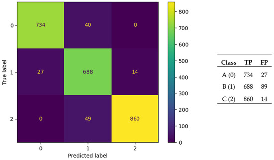
Figure 7.
Confusion matrix for the best-performing ANN (JA) for the gas-phase dataset.
The RoC curve drawn during the training of the best-performing ANN (JA) for the gas-phase dataset with 10-fold CV is given in Figure 8. For Class A, the mean AUC is 0.95; for Class B, the mean AUC is 0.87; and for Class C, the mean AUC is 0.94. The model performed very well in distinguishing Class A and Class C. The performance of the model for distinguishing Class B was slightly worse than that of the other two classes. For Class A and Class C, the variation in AUC scores in folds was very low, which indicated a stable performance. The AUC scores varied a bit more in folds for Class B, which indicated a less reliable classification performance. When we controlled the effect of the class imbalance, class imbalance was in the safe limits, with an Imbalance Ratio (IR) of 1.25:1 for the gas-phase dataset.
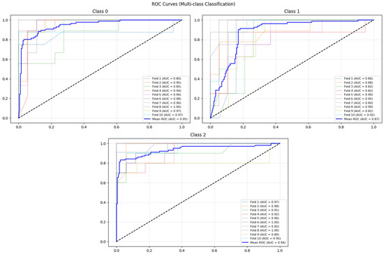
Figure 8.
RoC curve for the best-performing ANN (JA) for the gas phase dataset.
For the liquid-phase dataset, the best mean accuracy of 10-fold CV achieved by ANNs generated with JA and GA was 90.79%. The ANNs (ANN architectures) with the highest accuracies were discovered with JA, GA, and PSO optimizers. The metadata on architecture of the best-performing ANNs are given in Table 15 and Table 16. The confusion matrix for the best-performing ANNs is presented in Figure 9 and Figure 10 and it can be seen from these values that an accuracy rate of 90.79% was achieved.
Table 15.
The best-performing liquid-phase ANN architecture discovered with GA.
Table 16.
The best-performing liquid-phase ANN architecture discovered with JA.
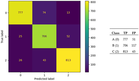
Figure 9.
Confusion matrix for the best-performing ANN (GA) for the liquid-phase dataset.
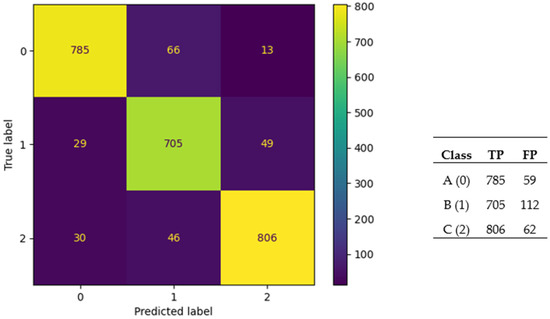
Figure 10.
Confusion matrix for the best-performing ANN (JA) for the liquid-phase dataset.
The RoC curve drawn during the training of the best-performing ANN (JA) for the liquid-phase dataset with 10-fold CV is given in Figure 11. For Class A, the mean AUC is 0.93; for Class B, the mean AUC is 0.87; and for Class C, the mean AUC is 0.94. The model performed very well in distinguishing Class A and Class C, similar to the results achieved in the gas-phase dataset. The performance of the model for distinguishing Class B was weaker, particularly for the first two folds, which achieved AUCs of 0.66 and 0.73, respectively. For Class A and Class C, the variation in the AUC scores in folds was very low, which indicated stable performance. The AUC scores varied greatly for some folds (e.g., between fold 1 and fold 9) for Class B which indicated a lower stability. When we controlled the effect of the class imbalance, class imbalance was in the safe limits, with an Imbalance Ratio (IR) of 1.13:1 for the liquid-phase dataset.

Figure 11.
RoC for the best-performing ANN (JA) for the liquid-phase dataset.
Figure 12 and Figure 13 show the confusion matrix for the worst-performing ANN (GA) for the gas-phase data set and the confusion matrix for the worst-performing ANN (PSO) for the liquid-phase data set. These two matrices are based on the results from the test folds.
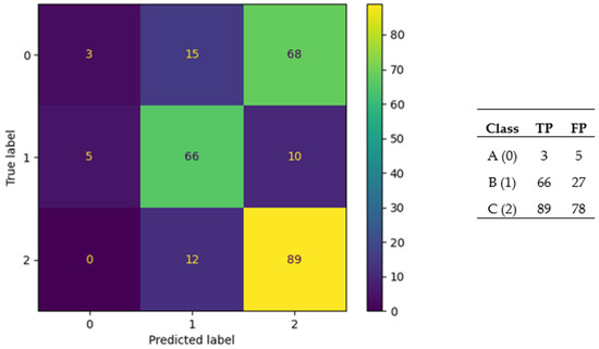
Figure 12.
Confusion matrix for the worst-performing ANN (GA) for the gas-phase dataset.
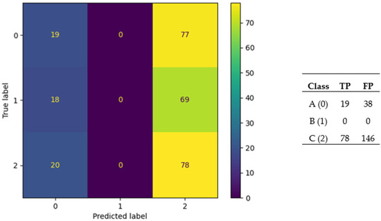
Figure 13.
Confusion matrix for the worst-performing ANN (PSO) for the liquid-phase dataset (34.52%).
For the gas-phase dataset, the worst-performing ANN was generated with the GA, and the best mean accuracy of 10-fold CV for this ANN was 58.96%. In this ANN, the majority of class A (0) was predicted as class C (2), and a considerable number of class A (0) and class C (2) were predicted as class B (1).The number of classes in the gas phase dataset were A:86, B:81, and C:101, the minor imbalance in classes where C > A,B may be the main reason behind the erroneous predictions.
For the liquid-phase dataset, the worst-performing ANN was generated with the PSO, and the best mean accuracy of 10-fold CV for this ANN was 34.52%. In this ANN, none of the predictions were class B (1); the majority of class A (0) was predicted as class C (2); similarly, the majority of class B (1) was predicted as class C (2). The numbers of classes in the gas-phase dataset were A:98, B:87, and C:96, and the minor imbalance in classes, where B < A,C, may have been the main reason behind the erroneous predictions.
In this study, to validate that the precision achieved by the ANNs discovered by HyperNetExplorer was significantly superior to the classical (well-known) ML algorithms, a series of training and tests was performed utilizing Scikit-Learn’s Decision Tree, Gaussian NB, K-Nearest Neighbors (KNN), Linear Discriminant Analysis (LDA), Support Vector Machine, Random Forest, Gradient Boosting, and Histogram Gradient Boosting algorithms, with 10-fold cross-validation. As explained in [116], despite the fact that deep-learning methods perform extremely well for classification on homogeneous data, the classification of tabular data is still a challenge for deep-learning models due to its heterogeneous nature, leading to a mix of dense numerical and sparse categorical features. This heterogeneity in tabular datasets, especially when the dataset contains lots of categorical features, each with lots of categories as in our dataset, results in a very weak correlation among the features when compared with the one introduced through spatial or semantic relationships in image or speech data. The reasons for failure of deep-learning models are strongly associated with the very nature of data, which mostly requires imputation, dealing with outlier and rebalancing of classes; furthermore, as there is often no spatial correlation between the variables, the dependencies between features are either complex or irregular. When working with tabular data, the learning algorithm has to learn the structure and relationships between its features from scratch. Thus, the reason behind the selection of classical (well-known) ML algorithms for comparison with the results obtained from HyperNetExplorer was the superior performance of the classical ML algorithms in tabular data classification problem when compared with modern deep learning methods. Table 17 below shows the accuracies obtained for each algorithm.
Table 17.
Machine-learning models.
The results of the testing with classical (well-known) ML algorithms demonstrate that the ANNs discovered with the HyperNetExplorer demonstrated significantly (200–250%) higher performance than that of the best-ranking classical ML algorithms of the Scikit-Learn package. Table 18 provides a summary of the studies in which hydrogen production is estimated using machine-learning methods.
Table 18.
A summary of studies on the estimation of hydrogen production with ML.
Studies that used regression-based ML approaches provided significantly good results by achieving R2 scores equal to or higher than 0.99 [3,5,36]. In fact, studies that used classification algorithms were unable to produce such successful accuracy rates. The highest classification accuracy that was observed in the literature was 92% [4]. In some datasets, the accuracy could be as low as 65% for a three-class classification problem. In ML, the accuracy rate is highly correlated with the nature of the dataset, and the number of classes, and to test if the accuracy can be improved, the same dataset should be used in comparisons of learning models.
In our study, we conducted our experiments with the same dataset as [1] to test whether we could improve the accuracy in datasets where low classification accuracy is persistent through the use of adaptive NAS and metaheuristics. In [1], the accuracy rates achieved with the implementation of a decision tree for the gas-phase dataset were 80% (for the training set) and 79% (for the test set); for the liquid-phase dataset, 77% (for the training set) and 65% (for the test set). Compared with [1], the accuracies achieved for the gas-phase dataset were 94% > 79%, and for the liquid-phase dataset, 90% > 65%, demonstrating that the discovery and use of fine-tuned ANN architectures through NAS greatly contribute to the classification accuracy of the total gas yield estimation in the photocatalytic CO2 reduction process.
4. Conclusions
Today, the amount of carbon dioxide is rapidly increasing due to reasons such as excessive consumption of fossil fuels and population growth. If this increase in the amount of carbon dioxide continues, extreme events, such as very high temperatures, droughts, and excessive precipitation, are inevitable. For this reason, methods to reduce the amount of carbon dioxide have gained importance in recent years. In this context, our study aimed to facilitate the reduction of CO2 (and the production of hydrogen) through a photocatalytic reaction. This study aimed to improve the estimation of the total gas yield (hydrogen production) of the photocatalysis process through NAS and hyperparameter optimization in ANNs. In this study, the dataset provided in [1] was used. At the beginning of our study, the source dataset was divided into two datasets according to the gas and liquid phases of the photocatalysis process. Later, data preprocessing (transformation, and imputation) was conducted on both datasets. Following this stage, we utilized HyperNetExplorer, a NAS tool to find the best ANN architecture that provides the most accurate prediction rates. The tests carried out with HyperNetExplorer resulted in the discovery of highly accurate ANN architectures in the estimation of the total gas (hydrogen) yield for the gas- and liquid-phase datasets. For the gas-phase dataset, we discovered an ANN architecture providing 94.61% classification accuracy, and for the liquid-phase dataset, an ANN architecture providing 90.79% classification accuracy was discovered. These values were significantly higher when compared with those of other well-known ML (such as decision trees and support vector machine) models and higher when compared with previous research [1]. The findings indicate that the discovery and use of fine-tuned ANNs greatly contributed to the prediction accuracy of the total gas (hydrogen) yield in the photocatalytic CO2 reduction process. The key limitation of this study was the experiment being conducted with a single dataset [1], future research will focus on validating the findings of this study with more datasets. Another dimension of this study was the use of HyperNetExplorer for finding the most accurate algorithms for estimating the total gas yield (hydrogen production) of the photocatalysis process. The ANN architectures are considered as foundational architectures when compared with CNN-based, RNN-based, or transformer-based architectures. In fact, the classification or regression-based estimation problems of tabular datasets benefitted much better from foundational ANN architectures, as fully connected neural network layers with their flexible and easily tunable parameters provide much better accuracy rates. This study provides a new neural architecture search implementation method, where the best hyperparameters of an ANN, such as the number of layers, number of neurons per layer, and activation functions per layer, can be determined as a result of searching by nearly a limitless number of optimizers. The key contribution of this study is the removal of the barrier of the need for tightly coupled hyperparameter optimization architectures, where hyperparameter optimization can only be conducted with a limited set of optimization algorithms provided by each hyperparameter optimization package. Instead, our implementation a new optimizer can be easily added to the MealPy package and the new optimizer can easily be used for optimization with a very simple adaptation in the code base.
The findings of this study will facilitate the estimation of the total gas yield in a photocatalytic CO2 reduction process. This will provide time and cost efficiency in the process, as the estimation of the total gas yield can be performed prior to the actual process, which will contribute to conducting feasibility studies without the need for conducting actual experiments, which are costly and time-consuming.
Author Contributions
Ü.I. and G.B. generated the analysis codes; Y.A., Ü.I. and G.B. developed the theory, background, and formulations of the problem; Verification of the results was performed by Y.A. and Ü.I.; The text of the paper was written by Y.A., Ü.I. and G.B.; The figures were drawn by Y.A.; Ü.I., G.B., S.A., J.H. and Z.W.G. edited the paper; Z.W.G. acquired fundings; G.B. and Z.W.G. supervised the research direction. All authors have read and agreed to the published version of the manuscript.
Funding
This work was supported by the Korea Institute of Energy Technology Evaluation and Planning (KETEP) and the Ministry of Trade, Industry & Energy, Republic of Korea (RS-2024-00442817). This work was also supported by the Gachon University research fund of 2024 (GCU-202403910001).
Institutional Review Board Statement
Not applicable.
Informed Consent Statement
Not applicable.
Data Availability Statement
Data are available on request to authors.
Conflicts of Interest
The authors declare no conflicts of interest.
References
- Saadetnejad, D.; Oral, B.; Can, E.; Yıldırım, R. Machine learning analysis of gas phase photocatalytic CO2 reduction for hydrogen production. Int. J. Hydrogen Energy 2022, 47, 19655–19668. [Google Scholar] [CrossRef]
- Ren, T.; Wang, L.; Chang, C.; Li, X. Machine learning-assisted multiphysics coupling performance optimization in a photocatalytic hydrogen production system. Energy Convers. Manag. 2020, 216, 112935. [Google Scholar] [CrossRef]
- Mageed, A.K. Modeling photocatalytic hydrogen production from ethanol over copper oxide nanoparticles: A comparative analysis of various machine learning techniques. Biomass Convers. Biorefin. 2021, 13, 3319–3327. [Google Scholar] [CrossRef]
- Ramkumar, G.; Tamilselvi, M.; Jebaseelan, S.S.; Mohanavel, V.; Kamyab, H.; Anitha, G.; Prabu, R.T.; Rajasimman, M. Enhanced machine learning for nanomaterial identification of photo thermal hydrogen production. Int. J. Hydrogen Energy 2024, 52, 696–708. [Google Scholar] [CrossRef]
- Yurova, V.Y.; Potapenko, K.O.; Aliev, T.A.; Kozlova, E.A.; Skorb, E.V. Optimization of g-C3N4 synthesis parameters based on machine learning to predict the efficiency of photocatalytic hydrogen production. Int. J. Hydrogen Energy 2024, 81, 193–203. [Google Scholar] [CrossRef]
- Wang, F.; Harindintwali, J.D.; Yuan, Z.; Wang, M.; Wang, F.; Li, S.; Yin, Z.; Huang, L.; Fu, Y.; Li, L.; et al. Technologies and perspectives for achieving carbon neutrality. Innovation 2021, 2, 100180. [Google Scholar] [CrossRef]
- Zohuri, B. Hydrogen Energy: Challenges and Solutions for a Cleaner Future; Springer International Publishing: Cham, Switzerland, 2019. [Google Scholar] [CrossRef]
- Da Rosa, A.V.; Ordonez, J.C. Fundamentals of Renewable Energy Processes; Academic Press: Cambridge, MA, USA, 2021. [Google Scholar]
- Olabi, A.G.; Abdelkareem, M.A. Renewable energy and climate change. Renew. Sustain. Energy Rev. 2022, 158, 112111. [Google Scholar] [CrossRef]
- Abbasi, K.R.; Shahbaz, M.; Zhang, J.; Irfan, M.; Alvarado, R. Analyze the environmental sustainability factors of China: The role of fossil fuel energy and renewable energy. Renew. Energy 2022, 187, 390–402. [Google Scholar] [CrossRef]
- Vivek, C.M.; Ramkumar, P.; Srividhya, P.K.; Sivasubramanian, M. Recent strategies and trends in implanting of renewable energy sources for sustainability–A review. Mater. Today Proc. 2021, 46, 8204–8208. [Google Scholar] [CrossRef]
- IEA. The Energy World Is Set to Change Significantly by 2030, Based on Today’s Policy Settings Alone. Available online: https://www.iea.org/news/the-energy-world-is-set-to-change-significantly-by-2030-based-on-today-s-policy-settings-alone (accessed on 20 July 2024).
- Average Monthly Carbon Dioxide (CO2) Levels in the Atmosphere Worldwide from 1990 to 2024. Available online: https://www.statista.com/statistics/1091999/atmospheric-concentration-of-co2-historic/#:~:text=Monthly%20mean%20atmospheric%20carbon%20dioxide,record%20high%20of%20421%20ppm (accessed on 22 July 2024).
- Basics of Climate Change. Available online: https://www.epa.gov/climatechange-science/basics-climate-change (accessed on 22 July 2024).
- Xu, X.; Zhou, Q.; Yu, D. The future of hydrogen energy: Bio-hydrogen production technology. Int. J. Hydrogen Energy 2022, 47, 33677–33698. [Google Scholar] [CrossRef]
- Hassan, Q.; Sameen, A.Z.; Salman, H.M.; Jaszczur, M.; Al-Jiboory, A.K. Hydrogen energy future: Advancements in storage technologies and implications for sustainability. J. Energy Storage 2023, 72, 108404. [Google Scholar] [CrossRef]
- Sharma, S.; Agarwal, S.; Jain, A. Significance of hydrogen as economic and environmentally friendly fuel. Energies 2021, 14, 7389. [Google Scholar] [CrossRef]
- Yue, M.; Lambert, H.; Pahon, E.; Roche, R.; Jemei, S.; Hissel, D. Hydrogen energy systems: A critical review of technologies, applications, trends and challenges. Renew. Sustain. Energy Rev. 2021, 146, 111180. [Google Scholar] [CrossRef]
- Penner, S.S. Steps toward the hydrogen economy. Energy 2006, 31, 33–43. [Google Scholar] [CrossRef]
- Hydrogen and Fuel Cell Technologies Office. Fuel Cells. Available online: https://www.energy.gov/eere/fuelcells/fuel-cells (accessed on 29 July 2024).
- International Renewable Energy Agency. Overview. Available online: https://www.irena.org/Energy-Transition/Technology/Hydrogen#:~:text=As%20at%20the%20end%20of,around%204%25%20comes%20from%20electrolysis (accessed on 11 November 2024).
- Aziz, M.; Darmawan, A.; Juangsa, F.B. Hydrogen production from biomasses and wastes: A technological review. Int. J. Hydrogen Energy 2021, 46, 33756–33781. [Google Scholar] [CrossRef]
- Arcos JM, M.; Santos, D.M. The hydrogen color spectrum: Techno-economic analysis of the available technologies for hydrogen production. Gases 2023, 3, 25–46. [Google Scholar] [CrossRef]
- Aydın, Y.; Işıkdağ, Ü.; Bekdaş, G.; Nigdeli, S.M.; Geem, Z.W. Use of machine learning techniques in soil classification. Sustainability 2023, 15, 2374. [Google Scholar] [CrossRef]
- Cakiroglu, C.; Aydın, Y.; Bekdaş, G.; Geem, Z.W. Interpretable predictive modelling of basalt fiber reinforced concrete splitting tensile strength using ensemble machine learning methods and SHAP approach. Materials 2023, 16, 4578. [Google Scholar] [CrossRef]
- Aydın, Y.; Bekdaş, G.; Nigdeli, S.M.; Isıkdağ, Ü.; Kim, S.; Geem, Z.W. Machine learning models for ecofriendly optimum design of reinforced concrete columns. Appl. Sci. 2023, 13, 4117. [Google Scholar] [CrossRef]
- Aydın, Y.; Cakiroglu, C.; Bekdaş, G.; Işıkdağ, Ü.; Kim, S.; Hong, J.; Geem, Z.W. Neural network predictive models for alkali-activated concrete carbon emission using metaheuristic optimization algorithms. Sustainability 2023, 16, 142. [Google Scholar] [CrossRef]
- Hu, G.; Liu, Y.; Chu, X.; Liu, Z. Fourier ptychographic layer-based imaging of hazy environments. Results Phys. 2024, 56, 107216. [Google Scholar] [CrossRef]
- Aydın, Y.; Cakiroglu, C.; Bekdaş, G.; Geem, Z.W. Explainable Ensemble Learning and Multilayer Perceptron modeling for compressive strength prediction of Ultra-high-performance concrete. Biomimetics 2024, 9, 544. [Google Scholar] [CrossRef] [PubMed]
- Cakiroglu, C.; Aydın, Y.; Bekdaş, G.; Isikdag, U.; Sadeghifam, A.N.; Abualigah, L. Cooling load prediction of a double-story terrace house using ensemble learning techniques and genetic programming with SHAP approach. Energy Build. 2024, 313, 114254. [Google Scholar] [CrossRef]
- Jayasinghe, T.; Chen, B.W.; Zhang, Z.; Meng, X.; Li, Y.; Gunawardena, T.; Mangalathu, S.; Mendis, P. Data-driven shear strength predictions of recycled aggregate concrete beams with/without shear reinforcement by applying machine learning approaches. Constr. Build. Mater. 2023, 387, 131604. [Google Scholar] [CrossRef]
- Qiu, W.X.; Si, Z.Z.; Mou, D.S.; Dai, C.Q.; Li, J.T.; Liu, W. Data-driven vector degenerate and nondegenerate solitons of coupled nonlocal nonlinear Schrödinger equation via improved PINN algorithm. Nonlinear Dyn. 2024, 1–14. [Google Scholar] [CrossRef]
- Olyanasab, A.; Annabestani, M. Leveraging Machine Learning for Personalized Wearable Biomedical Devices: A Review. J. Pers. Med. 2024, 14, 203. [Google Scholar] [CrossRef]
- Yan, L.; Zhong, S.; Igou, T.; Gao, H.; Li, J.; Chen, Y. Development of machine learning models to enhance element-doped g-C3N4 photocatalyst for hydrogen production through splitting water. Int. J. Hydrogen Energy 2022, 47, 34075–34089. [Google Scholar] [CrossRef]
- Xu, Y.; Ju, C.W.; Li, B.; Ma, Q.S.; Chen, Z.; Zhang, L.; Chen, J. Hydrogen evolution prediction for alternating conjugated copolymers enabled by machine learning with multidimension fragmentation descriptors. ACS Appl. Mater. Interfaces 2021, 13, 34033–34042. [Google Scholar] [CrossRef]
- Haq, Z.U.; Ullah, H.; Khan MN, A.; Naqvi, S.R.; Ahsan, M. Hydrogen production optimization from sewage sludge supercritical gasification process using machine learning methods integrated with genetic algorithm. Chem. Eng. Res. Des. 2022, 184, 614–626. [Google Scholar] [CrossRef]
- Ajmal, Z.; Haq, M.U.; Naciri, Y.; Djellabi, R.; Hassan, N.; Zaman, S.; Murtaza, A.; Kumar, A.; Al-Sehemi, A.G.; Algarni, H.; et al. Recent advancement in conjugated polymers based photocatalytic technology for air pollutants abatement: Cases of CO2, NOx, and VOCs. Chemosphere 2022, 308, 136358. [Google Scholar] [CrossRef]
- Abbas, A.M.; Hammad, S.A.; Sallam, H.; Mahfouz, L.; Ahmed, M.K.; Abboudy, S.M.; Ahmed, A.E.; Alhag, S.K.; Taher, M.A.; Alrumman, S.A.; et al. Biosynthesis of zinc oxide nanoparticles using leaf extract of Prosopis juliflora as potential photocatalyst for the treatment of paper mill effluent. Appl. Sci. 2021, 11, 11394. [Google Scholar] [CrossRef]
- Mohanty, S.; Moulick, S.; Maji, S.K. Adsorption/photodegradation of crystal violet (basic dye) from aqueous solution by hydrothermally synthesized titanate nanotube (TNT). J. Water Process Eng. 2020, 37, 101428. [Google Scholar] [CrossRef]
- Lofrano, G.; Ubaldi, F.; Albarano, L.; Carotenuto, M.; Vaiano, V.; Valeriani, F.; Libralato, G.; Gianfranceschi, G.; Fratoddi, I.; Meric, S.; et al. Antimicrobial effectiveness of innovative photocatalysts: A review. Nanomaterials 2022, 12, 2831. [Google Scholar] [CrossRef] [PubMed]
- Chang, J.; Ma, J.; Ma, Q.; Zhang, D.; Qiao, N.; Hu, M.; Ma, H. Adsorption of methylene blue onto Fe3O4/activated montmorillonite nanocomposite. Appl. Clay Sci. 2016, 119, 132–140. [Google Scholar] [CrossRef]
- Bhom, F.; Isa, Y.M. Photocatalytic Hydrogen Production Using TiO2-based Catalysts: A Review. Glob. Chall. 2024, 8, 2400134. [Google Scholar] [CrossRef] [PubMed]
- Ma, Y.; Wang, X.; Jia, Y.; Chen, X.; Han, H.; Li, C. Titanium dioxide-based nanomaterials for photocatalytic fuel generations. Chem. Rev. 2014, 114, 9987–10043. [Google Scholar] [CrossRef]
- Chen, D.; Cheng, Y.; Zhou, N.; Chen, P.; Wang, Y.; Li, K.; Huo, S.; Cheng, P.; Peng, P.; Zhang, R.; et al. Photocatalytic degradation of organic pollutants using TiO2-based photocatalysts: A review. J. Clean. Prod. 2020, 268, 121725. [Google Scholar] [CrossRef]
- Xia, C.; Nguyen, T.H.C.; Nguyen, X.C.; Kim, S.Y.; Nguyen, D.L.T.; Raizada, P.; Singh, P.; Nguyen, V.-H.; Nguyen, C.C.; Hoang, V.C.; et al. Emerging cocatalysts in TiO2-based photocatalysts for light-driven catalytic hydrogen evolution: Progress and perspectives. Fuel 2022, 307, 121745. [Google Scholar] [CrossRef]
- Arora, I.; Chawla, H.; Chandra, A.; Sagadevan, S.; Garg, S. Advances in the strategies for enhancing the photocatalytic activity of TiO2: Conversion from UV-light active to visible-light active photocatalyst. Inorg. Chem. Commun. 2022, 143, 109700. [Google Scholar] [CrossRef]
- Albahra, S.; Gorbett, T.; Robertson, S.; D’Aleo, G.; Kumar, S.V.S.; Ockunzzi, S.; Lallo, D.; Hu, B.; Rashidi, H.H. Artificial intelligence and machine learning overview in pathology & laboratory medicine: A general review of data preprocessing and basic supervised concepts. In Seminars in Diagnostic Pathology; WB Saunders: Philadelphia, PA, USA, 2023; Volume 40, pp. 71–87. [Google Scholar] [CrossRef]
- Tawakuli, A.; Havers, B.; Gulisano, V.; Kaiser, D.; Engel, T. Survey: Time-series data preprocessing: A survey and an empirical analysis. J. Eng. Res. 2024. [Google Scholar] [CrossRef]
- García, S.; Luengo, J.; Herrera, F. Data Preprocessing in Data Mining; Springer International Publishing: Cham, Switzerland, 2015; Volume 72, pp. 59–139. [Google Scholar] [CrossRef]
- Python (3.9) [Computer Software]. Available online: http://python.org (accessed on 5 August 2024).
- Anaconda3 [Computer Software]. Available online: https://anaconda.org/ (accessed on 5 August 2024).
- Raybaut, P. Spyder-Documentation. 2009. Available online: https://www.spyder-ide.org/ (accessed on 7 August 2024).
- Harris, C.R.; Millman, K.J.; Van Der Walt, S.J.; Gommers, R.; Virtanen, P.; Cournapeau, D.; Wieser, E.; Taylor, J.; Berg, S.; Smith, N.J.; et al. Array programming with NumPy. Nature 2020, 585, 357–362. [Google Scholar] [CrossRef] [PubMed]
- About Pandas. Available online: https://pandas.pydata.org/ (accessed on 7 August 2024).
- Pedregosa, F.; Varoquaux, G.; Gramfort, A.; Michel, V.; Thirion, B.; Grisel, O.; Blondel, M.; Prettenhofer, P.; Weiss, R.; Dubourg, V. Scikit-learn: Machine learning in Python. J. Mach. Learn. Res. 2011, 12, 2825–2830. [Google Scholar]
- Ma, Y.; Zhang, Z. Travel mode choice prediction using deep neural networks with entity embeddings. IEEE Access 2020, 8, 64959–64970. [Google Scholar] [CrossRef]
- Yedla, A.; Kakhki, F.D.; Jannesari, A. Predictive modeling for occupational safety outcomes and days away from work analysis in mining operations. Int. J. Environ. Res. Public Health 2020, 17, 7054. [Google Scholar] [CrossRef]
- Hale, T.; Angrist, N.; Goldszmidt, R.; Kira, B.; Petherick, A.; Phillips, T.; Webster, S.; Cameron-Blake, E.; Hallas, L.; Majumdar, S.; et al. A global panel database of pandemic policies (Oxford COVID-19 Government Response Tracker). Nat. Hum. Behav. 2021, 5, 529–538. [Google Scholar] [CrossRef]
- Bennett, D.A. How can I deal with missing data in my study? Aust. N. Z. J. Public Health 2001, 25, 464–469. [Google Scholar] [CrossRef]
- Schafer, J.L. Multiple imputation: A primer. Statistical methods in medical research 1999, 8, 3–15. Schafer, J.L. Multiple imputation: A primer. Stat. Methods Med. Res. 1999, 8, 3–15. [Google Scholar] [CrossRef]
- Mealpy. Available online: https://github.com/thieu1995/mealpy (accessed on 8 August 2024).
- Lima, A.A.; Mridha, M.F.; Das, S.C.; Kabir, M.M.; Islam, M.R.; Watanobe, Y. A comprehensive survey on the detection, classification, and challenges of neurological disorders. Biology 2022, 11, 469. [Google Scholar] [CrossRef]
- McUlloch, W.S.; Pitts, W. A Logical Calculus of the Ideas Immanent in Nervous Activity. Bull. Math. Biophys. 1943, 5, 115–133. [Google Scholar] [CrossRef]
- Öztemel, E. Artificial Neural Networks, 3rd ed.; Papatya Publishing Education: Istanbul, Turkey, 2012. [Google Scholar]
- Calandra, H.; Gratton, S.; Riccietti, E.; Vasseur, X. On a multilevel Levenberg–Marquardt method for the training of artificial neural networks and its application to the solution of partial differential equations. Optim. Methods Softw. 2022, 37, 361–386. [Google Scholar] [CrossRef]
- Panimalar, S.A.; Krishnakumar, A. Customer churn prediction model in cloud environment using DFE-WUNB: ANN deep feature extraction with weight updated tuned Naïve bayes classification with block-jacobi SVD dimensionality reduction. Eng. Appl. Artif. Intell. 2023, 126, 107015. [Google Scholar] [CrossRef]
- Yalçın, O.G. Deep learning and neural networks overview. In Applied Neural Networks with Tensorflow 2: API oriented Deep Learning with Python; Apress: New York, NY, USA, 2021; pp. 57–80. [Google Scholar] [CrossRef]
- Uma, U.U.; Nmadu, D.; Ugwuanyi, N.; Ogah, O.E.; Eli-Chukwu, N.; Eheduru, M.; Ekwue, A. Adaptive overcurrent protection scheme coordination in presence of distributed generation using radial basis neural network. Prot. Control Mod. Power Syst. 2023, 8, 1–19. [Google Scholar] [CrossRef]
- Gülcü, A.; Kuş, Z. A Survey of Hyper-parameter Optimization Methods in Convolutional Neural Networks. Gazi Univ. J. Sci. 2019, 7, 503–522. [Google Scholar] [CrossRef]
- Misra, D. Mish: A self regularized non-monotonic activation function. arXiv 2019, arXiv:1908.08681. [Google Scholar] [CrossRef]
- Clevert, D.A.; Unterthiner, T.; Hochreiter, S. Fast and accurate deep network learning by exponential linear units (elus). arXiv 2015, arXiv:1511.07289. [Google Scholar]
- Yang, X.S. Flower pollination algorithm for global optimization. In Proceedings of the International Conference on Unconventional Computing and Natural Computation, Orléan, France, 3–7 September 2012; Springer: Berlin/Heidelberg, Germany, 2012; pp. 240–249. [Google Scholar] [CrossRef]
- Albadr, M.A.; Tiun, S.; Ayob, M.; Al-Dhief, F. Genetic algorithm based on natural selection theory for optimization problems. Symmetry 2020, 12, 1758. [Google Scholar] [CrossRef]
- Xue, Y.; Zhu, H.; Liang, J.; Słowik, A. Adaptive crossover operator based multi-objective binary genetic algorithm for feature selection in classification. Knowl.-Based Syst. 2021, 227, 107218. [Google Scholar] [CrossRef]
- Geem, Z.W.; Kim, J.H.; Loganathan, G.V. A new heuristic optimization algorithm: Harmony search. Simulation 2001, 76, 60–68. [Google Scholar] [CrossRef]
- Rao, R. Jaya: A simple and new optimization algorithm for solving constrained and unconstrained optimization problems. Int. J. Ind. Eng. Comput. 2016, 7, 19–34. [Google Scholar] [CrossRef]
- Kennedy, J.; Eberhart, R. Particle swarm optimization. In Proceedings of the ICNN’95-International Conference on Neural Networks, Perth, WA, Australia, 27 November–1 December 1995; IEEE: New York, NY, USA, 1995; Volume 4, pp. 1942–1948. [Google Scholar]
- Rao, R.V.; Savsani, V.J.; Vakharia, D.P. Teaching–learning-based optimization: A novel method for constrained mechanical design optimization problems. Comput.-Aided Des. 2011, 43, 303–315. [Google Scholar] [CrossRef]
- Chen, Y.; Pi, D. An innovative flower pollination algorithm for continuous optimization problem. Appl. Math. Model. 2020, 83, 237–265. [Google Scholar] [CrossRef]
- Nancy, M.; Stephen SE, A. A comprehensive review on harmony search algorithm. Ann. Rom. Soc. Cell Biol. 2021, 25, 5480–5483. [Google Scholar]
- Bellman, R.E.; Dreyfus, S.E. Applied Dynamic Programming; Princeton University Press: Princeton, NJ, USA, 2015. [Google Scholar] [CrossRef]
- Li, W.; He, Z.; Zheng, J.; Hu, Z. Improved flower pollination algorithm and its application in user identification across social networks. IEEE Access 2019, 7, 44359–44371. [Google Scholar] [CrossRef]
- What Is The Time Complexity Of A Genetic Algorithm? Available online: https://www.ontechnos.com/the-time-complexity-of-a-genetic-algorithm (accessed on 25 November 2024).
- Tian, Z.; Zhang, C. An improved harmony search algorithm and its application in function optimization. J. Inf. Process. Syst. 2018, 14, 1237–1253. [Google Scholar] [CrossRef]
- Shingade, S.; Niyogi, R.; Pichare, M. Hybrid Particle Swarm Optimization-Jaya Algorithm for Team Formation. Algorithms 2024, 17, 379. [Google Scholar] [CrossRef]
- Zhang, X.; Zou, D.; Shen, X. A novel simple particle swarm optimization algorithm for global optimization. Mathematics 2018, 6, 287. [Google Scholar] [CrossRef]
- Dastan, M.; Shojaee, S.; Hamzehei-Javaran, S.; Goodarzimehr, V. Hybrid teaching–learning-based optimization for solving engineering and mathematical problems. J. Braz. Soc. Mech. Sci. Eng. 2022, 44, 431. [Google Scholar] [CrossRef]
- Yadav, S.; Shukla, S. Analysis of k-fold cross-validation over hold-out validation on colossal datasets for quality classification. In Proceedings of the 2016 IEEE 6th International Conference on Advanced Computing (IACC), Bhimavaram, India, 27–28 February 2016; IEEE: New York, NY, USA; pp. 78–83. [Google Scholar] [CrossRef]
- Talukder, M.A.; Islam, M.M.; Uddin, M.A.; Akhter, A.; Hasan, K.F.; Moni, M.A. Machine learning-based lung and colon cancer detection using deep feature extraction and ensemble learning. Expert Syst. Appl. 2022, 205, 117695. [Google Scholar] [CrossRef]
- Zhao, L.; Lee, S.; Jeong, S.P. Decision tree application to classification problems with boosting algorithm. Electronics 2021, 10, 1903. [Google Scholar] [CrossRef]
- Winterburn, J.L.; Voineskos, A.N.; Devenyi, G.A.; Plitman, E.; de la Fuente-Sandoval, C.; Bhagwat, N.; Graff-Guerrero, A.; Knight, J.; Chakravarty, M.M. Can we accurately classify schizophrenia patients from healthy controls using magnetic resonance imaging and machine learning? A multi-method and multi-dataset study. Schizophr. Res. 2019, 214, 3–10. [Google Scholar] [CrossRef]
- Yacouby, R.; Axman, D. Probabilistic Extension of Precision, Recall, and F1 Score for More Thorough Evaluation of Classification Models. In Proceedings of the First Workshop on Evaluation and Comparison of NLP Systems, Online, 20 November 2020; pp. 79–91. [Google Scholar] [CrossRef]
- Derczynski, L. Complementarity, F-score, and NLP Evaluation. In Proceedings of the Tenth International Conference on Language Resources and Evaluation (LREC’16), Portorož, Slovenia, 23–28 May 2016; pp. 261–266. [Google Scholar]
- Paszke, A.; Gross, S.; Massa, F.; Lerer, A.; Bradbury, J.; Chanan, G.; Killeen, T.; Lin, Z.; Gimelshein, N.; Antiga, L.; et al. Pytorch: An imperative style, high-performance deep learning library. Adv. Neural Inf. Process. Syst. 2019, 32. [Google Scholar] [CrossRef]
- HyperNetExplorer. Available online: https://hyperopt.streamlit.app (accessed on 11 August 2024).
- Van Thieu, N.; Mirjalili, S. MEALPY: An open-source library for latest meta-heuristic algorithms in Python. J. Syst. Archit. 2023, 139, 102871. [Google Scholar] [CrossRef]
- Van Thieu, N.; Barma, S.D.; Van Lam, T.; Kisi, O.; Mahesha, A. Groundwater level modeling using augmented artificial ecosystem optimization. J. Hydrol. 2023, 617, 129034. [Google Scholar] [CrossRef]
- Ahmed, A.N.; Van Lam, T.; Hung, N.D.; Van Thieu, N.; Kisi, O.; El-Shafie, A. A comprehensive comparison of recent developed meta-heuristic algorithms for streamflow time series forecasting problem. Appl. Soft Comput. 2021, 105, 107282. [Google Scholar] [CrossRef]
- Dorogush, A.V.; Ershov, V.; Gulin, A. CatBoost: Gradient boosting with categorical features support. arXiv 2018, arXiv:1810.11363. [Google Scholar]
- Bibal, A.; Delchevalerie, V.; Frénay, B. DT-SNE: T-SNE discrete visualizations as decision tree structures. Neurocomputing 2023, 529, 101–112. [Google Scholar] [CrossRef]
- Assis, A.; Véras, D.; Andrade, E. Explainable Artificial Intelligence-An Analysis of the Trade-offs Between Performance and Explainability. In Proceedings of the 2023 IEEE Latin American Conference on Computational Intelligence (LA-CCI), Recife, Brazil, 29 October–1 November 2023; IEEE: New York, NY, USA; pp. 1–6. [Google Scholar] [CrossRef]
- Cheraghi, Y.; Kord, S.; Mashayekhizadeh, V. Application of machine learning techniques for selecting the most suitable enhanced oil recovery method; challenges and opportunities. J. Pet. Sci. Eng. 2021, 205, 108761. [Google Scholar] [CrossRef]
- Shobha, G.; Rangaswamy, S. Chapter 8—Machine Learning Handbook of Statistics; Elsevier: Amsterdam, The Netherlands. [CrossRef]
- Özbay Karakuş, M.; Er, O. A comparative study on prediction of survival event of heart failure patients using machine learning algorithms. Neural Comput. Appl. 2022, 34, 13895–13908. [Google Scholar] [CrossRef]
- Halder, R.K.; Uddin, M.N.; Uddin, M.A.; Aryal, S.; Khraisat, A. Enhancing K-nearest neighbor algorithm: A comprehensive review and performance analysis of modifications. J. Big Data 2024, 11, 113. [Google Scholar] [CrossRef]
- Qu, L.; Pei, Y. A Comprehensive Review on Discriminant Analysis for Addressing Challenges of Class-Level Limitations, Small Sample Size, and Robustness. Processes 2024, 12, 1382. [Google Scholar] [CrossRef]
- Lewis, D.N. Machine Learning Made Easy with R: An Intuitive Step by Step Blueprint for Beginners; CreateSpace Independent Publishing Platform: Scotts Valley, CA, USA, 2017. [Google Scholar]
- Anowar, F.; Sadaoui, S.; Selim, B. Conceptual and empirical comparison of dimensionality reduction algorithms (pca, kpca, lda, mds, svd, lle, isomap, le, ica, t-sne). Comput. Sci. Rev. 2021, 40, 100378. [Google Scholar] [CrossRef]
- Alp Aydin, E. Introduction to Machine Learning; MIT Press: Cambridge, MA, USA, 2020; ISBN 9780262043793. [Google Scholar]
- Breiman, L. Bagging predictors. Mach. Learn. 1996, 24, 123–140. [Google Scholar] [CrossRef]
- Robert, N.; Gary, M.; Ken, Y. (Eds.) Chapter 9—Classification. In Handbook of Statistical Analysis and Data Mining Applications, 2nd ed.; Academic Press: Cambridge, MA, USA, 2018; pp. 169–186. ISBN 9780124166325. [Google Scholar] [CrossRef]
- Kiangala, S.K.; Wang, Z. An effective adaptive customization framework for small manufacturing plants using extreme gradient boosting-XGBoost and random forest ensemble learning algorithms in an Industry 4.0 environment. Mach. Learn. Appl. 2021, 4, 100024. [Google Scholar] [CrossRef]
- Guryanov, A. Histogram-based algorithm for building gradient boosting ensembles of piecewise linear decision trees. In Proceedings of the Analysis of Images, Social Networks and Texts: 8th International Conference, AIST 2019, Kazan, Russia, 17–19 July 2019; Revised Selected Papers 8. Springer International Publishing: Cham, Switzerland; pp. 39–50. [Google Scholar] [CrossRef]
- Features in Histogram Gradient Boosting Trees. Available online: https://scikit-learn.org/1.5/auto_examples/ensemble/plot_hgbt_regression.html (accessed on 11 November 2024).
- Parameter Tuning. Available online: https://catboost.ai/en/docs/concepts/parameter-tuning (accessed on 11 November 2024).
- Borisov, V.; Leemann, T.; Seßler, K.; Haug, J.; Pawelczyk, M.; Kasneci, G. Deep neural networks and tabular data: A survey. IEEE Trans. Neural Netw. Learn. Syst. 2022, 35, 7499–7519. [Google Scholar] [CrossRef]


Disclaimer/Publisher’s Note: The statements, opinions and data contained in all publications are solely those of the individual author(s) and contributor(s) and not of MDPI and/or the editor(s). MDPI and/or the editor(s) disclaim responsibility for any injury to people or property resulting from any ideas, methods, instructions or products referred to in the content. |
© 2024 by the authors. Licensee MDPI, Basel, Switzerland. This article is an open access article distributed under the terms and conditions of the Creative Commons Attribution (CC BY) license (https://creativecommons.org/licenses/by/4.0/).