1. Introduction
The importance of optimization processes connected to trailers at intermodal terminals is increasing with the growing amount of transport carried out by road tractors with trailers inside the European Union (EU). In 2021, road tractors with trailers dominated the road freight transport sector in 17 EU countries, contributing to more than 60% of the total tonne-kilometers conducted at the national level [
1]. As for railroad freight transportation, compared to 2009, the volume of goods transported via intermodal rail freight in Europe witnessed a significant increase of 49.9% in tonnage [
2]. Such a growing use of trailers is crucial for the environment. Inland ports, vital links between the hinterland and maritime shipping routes, not only facilitate the efficient movement of goods but also contribute to reducing CO
2 emissions [
3]. It is for this reason that the role of intermodal terminals is only increasing in the current worldwide situation when pollution intensifies and carbon dioxide emissions from transportation emerge as a major environmental challenge [
4,
5]. The automated damage detection (ADD) algorithm proposed in this paper is one of the highly desired process innovations by many intermodal terminals that will help not only optimize internal operations but also positively impact the achievement of the terminal’s environmental targets in the long run.
At the same time, the integration of ADD will alleviate the considerable workload on professional checkers, who can then be reallocated to carry out other important tasks. Thus, upon arrival at the terminal, the damaged trailer will be identified within a few seconds and redirected to the repair area without subsequently blocking the movement of other trucks. Such a significant reduction in unnecessary trailer movements will help substantially decrease the amount of CO
2 emissions at terminals, which is extremely important for combating the greenhouse effect. Since most terminals already have optical character recognition (OCR) gates, our developed ADD algorithm is an attractive process improvement step that can significantly reduce financial and time costs for many intermodal terminals worldwide. This is crucial in the current situation where the high cost of personnel constitutes one of the barriers to popularizing inland intermodal transportation [
6]. Investments into such an innovative and interactive solution may become a new source of competitive advantage for terminal operators [
7]. There are several motives to develop and integrate such an improvement into a terminal’s information ecosystem [
8]:
Advancing the automation process.
Enhancing terminal offerings by proposing fast and reliable solutions to handle damaged trailers.
Documenting and protecting against claims: all detection results will be stored in the Terminal Operating System (TOS) and can be accessed promptly in case of claims for compensation.
Currently, OCR gates save images of trailers from all sides in the terminal operating system (TOS) for manual documentation of detected damages post-factum. Simultaneously, an ADD algorithm may analyze them online with pre-trained neural networks (NNs).
At present, the ADD of trailers is a highly under-researched field. In contrast, ADD based on deep learning is well-investigated for other domains, e.g., maritime transportation with containers. To the best of our knowledge, the first published attempt to transfer several techniques for ADD from these domains to trailers was made by Cimili et al. [
9]. Their experiments were performed using the MobileNetV2 [
10] network based on transfer learning and convolutional autoencoders (CAE) for semi-supervised classification. Nevertheless, none of these approaches, which showed high efficiency in detecting container defects, could achieve similar performance for trailer damage detection.
This is related to the particularity of the surface structure of trailers and containers. While containers feature a modular design with corrugated metal walls for increased strength and stacking capabilities, trailers typically possess a continuous soft tarpaulin surface. In addition, trailers are equipped with belts (tie-downs) along their sides, which are not present on containers. Thus, trailers are susceptible to types of damage not inherent to containers: cracked tarpaulin, torn belts, missing belts, and improper tarpaulin patches (
Figure 1).
The aim of this paper is to find a novel ADD approach specifically for trailers that goes beyond knowledge transfer from other domains like the ADD of containers.
To reach this aim, we developed an algorithm based on ensemble learning, which achieves 88.33% accuracy and 81.08% F1-Score on the test data. For different tasks of the algorithm RetinaNet [
11], YOLOv8 [
12], and Faster R-CNN [
13] were tested, and the best-performing network was selected for every task.
The contributions of this paper are summarized as follows:
Introduction of a novel ensemble deep learning algorithm designed explicitly for the ADD of trailers at terminals. To the best of our knowledge, this is the first published algorithm that can handle damage detection of trailers using full-sized real-world OCR images of trailers.
Comprehensive testing of several state-of-the-art object detection deep neural networks in the ADD ensemble framework.
The proposal and testing of an alternative algorithm of trailer detection on the image using only classical computer vision techniques without deep learning.
Analysis and recommendations for the ADD improvement for a specific terminal, which was a part of this study. While derived from a particular case study, these recommendations are applicable to any terminal worldwide that seeks to integrate a similar ADD algorithm.
The paper is structured as follows:
Section 2 will provide an overview of the current state of the art in the field of object detection and its usage in previous papers on the automation of damage assessment. Then we describe the ensemble learning algorithm and the used data in
Section 3. In
Section 4, we show the performance of the developed algorithm. Finally, the conclusions are provided in
Section 5.
2. State of the Art
Cimili et al. [
9] were the first to test several approaches for the ADD of trailers. The first was based on a semi-supervised deep learning approach based on a Residual Encoder–Decoder Network [
14] or inception-like CAE [
15]. The idea was to train the autoencoders exclusively on the images of the negative, non-damaged class. Thus, the autoencoder could never learn any patterns of the damage and could not reproduce them. Afterward, the threshold based on the similarity of input and output images was determined. If the similarity was below the threshold, the image was classified as “damaged”. However, the method did not work robustly. One of the main reasons for the high misclassification rate was the lack of images of the negative class in the training set that could represent cases very similar to the positive class, i.e., improper patches, scratches, and twisted belts. As semi-supervised learning did not yield desirable results, the authors turned to supervised learning, namely, to the subclass of supervised learning called transfer learning. For that, they used convolutional NN MobileNetV2 [
10], which had already been pretrained on large datasets by the model’s authors. Despite the data not being directly related to trailers or containers, this transfer of knowledge could help in the identification of specific shapes and patterns and could help to cover the lack of the training data. The approach showed the most promising results, achieving more than 85% precision and accuracy on the test set consisting of image tiles. However, these results were not good enough to perform testing on the full-sized trailer images; all of them would be classified as “damaged” as at least 10% of the image tiles with the model’s performance would be misclassified.
Our goal is to advance the groundwork laid by Cimili et al. [
9] by developing an improved ADD algorithm. However, in this work, we perform tests not only on tiles but on the full trailer images, which is crucial from a practical point of view for real-world implementation. While we utilize several valuable concepts and ideas from Cimili et al. [
9], we have enhanced and implemented them within the framework of an ensemble learning approach known as the “bucket of models”, where different models are trained and tested for various purposes, and the best one is selected for each task.
Usually, one-stage and two-stage detectors are used for object detection in ensemble learning tasks. In our research, we tested both types of detectors.
The vanilla version of the Region-based Convolutional Neural Network (R-CNN), one of the most used two-stage algorithms, was presented by Girshick et al. [
16]. The main disadvantage of this network was its slowness. It is for this reason that one year later, Girshick [
17] proposed an improved version of the algorithm called Fast R-CNN with a single convolutional module. Finally, the same year, Faster R-CNN was released [
13]. It has a separate Region Proposal Network (RPN) for region proposal generation, dramatically decreasing the time required for object detection. Faster R-CNN has already been successfully tested for different damage detection tasks, e.g., road damage detection [
18] and classification [
19]. A particular version of R-CNN, Mask R-CNN, is used for the damage segmentation of containers [
20] and cars [
21], which further suggests the effectiveness of the algorithm for this type of task.
The main characteristic of one-stage detectors is that they skip the step of region proposal and return bounding boxes in a shorter time, which is crucial for real-world applications. “You Only Look Once” (YOLO) is an example of such an algorithm. One of its last releases, YOLOv8, outperforms efficient predecessors YOLOv3 [
22] and YOLOv5 [
23] in speed and accuracy [
12]. YOLO proved its efficiency for damage detection in many studies ([
18,
24,
25,
26]).
Another one-stage detection algorithm used in this research is RetinaNet [
11]. It consists of two major parts, one for classifying predictions and another for predicting bounding boxes. The main advantage of the algorithm is its focal loss, which handles class imbalance very well. It showed high performance in road damage detection and even outperformed Faster R-CNN and different YOLO versions [
25,
27]. RetinaNet demonstrated high performance for the trailer detection task in Cimili et al. [
9].
Slice-aided hyper inference (SAHI) is applied to handle object detection on large images [
28]. The approach helps to divide a large image into tiles for training and to perform inference of the trained detector. It delivers higher accuracy, faster computational time, and less hardware loads for making predictions on high-resolution images. SAHI is perfectly compatible with YOLOv8 and all the models from the Detectron2 package [
29]. A combination of SAHI and YOLOv5 was successfully tested for damage detection for hardwood floors [
30].
To the best of our knowledge, integrating the aforementioned object detection networks within an ensemble learning framework and implementing SAHI techniques tailored explicitly for trailers has not been explored or documented in any published papers yet. To address this research gap, we present our ensemble learning architecture, data, training and testing environment, and the computational results in the following sections.
3. Material and Methods
The study was based on data provided by a single multimodal freight operator. All the experiments were run on the computer equipped with AMD Ryzen 5 5600, NVIDIA GeForce RTX 3060 12 GB, 32 GB RAM DDR4 3200 MHz, and Windows 10 as the operating system. Besides the Detectron2, SAHI, imgaug, and Ultralytics packages, we also used Keras, Tensorflow, opencv-python, matplotlib, and scikit-image libraries.
The dataset used in this research (publicly unavailable due to privacy restrictions) consisted of unlabelled real-world images of the left and right sides of the trailers taken at the OCR gate at the entrance of an inland intermodal terminal in Europe. The spatial resolution of the images was volatile. While the height was always 2000 pixels, the width varied between approximately 7000 and 12,000 pixels, as shown in
Figure 2. With the current technology of the OCR gate, it was impossible to standardize the image width, as it depended on the speed of the truck driving through the gate.
The trailers’ pictures included unnecessary background details that could affect the ADD. To remove this background, we decided to crop trailers from images, which solved several issues simultaneously:
Reduced the size of the training set—irrelevant backgrounds such as wheels, driver’s cabins, or fuel tanks were excluded.
Increased inference speed—the trained NN for damage detection did not need to analyze excluded backgrounds.
Reduced the number of false positive (FP) predictions—given the similarity in appearance among all the trailers, diverse models of trucks and wheels exist. Consequently, the ADD might be unable to accurately learn all objects that may belong to the background and would incorrectly identify some of these objects as “damage”.
For the different phases of the ensemble learning model, we chose one modification of the one-stage algorithms YOLOv8 and RetinaNet, RetinaNet R101 and YOLOv8l, and one modification of the two-stage detection algorithm Faster R-CNN, Faster R-CNN R101-FPN. The main criteria for the selection were performance and hardware restrictions. For working with Faster R-CNN R101-FPN and RetinaNetR101, we used the Detectron2 package, while YOLOv8l was trained with the Ultralitycs package.
During the YOLOv8 training, the complex loss function was used. It consists of two major components—VarifocalLoss and SIoU Loss. VarifocalLoss is a refined version of the traditional focal loss, which manages class imbalance. Simultaneously, SIoU Loss improves the prediction of bounding boxes by evaluating different geometrical factors like angle and shape discrepancies between the ground truth and predicted bounding boxes. The abovementioned classical focal loss was used for the training of RetinaNet. For the Faster R-CNN training, we used the combination of the L1-loss and the binary cross entropy loss.
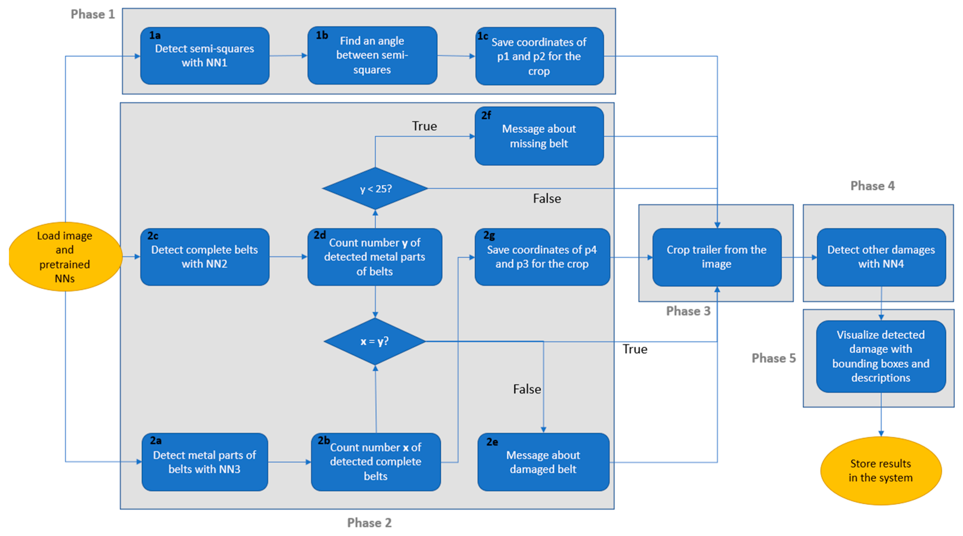
The entire process of ADD based on ensemble learning consists of multiple phases, including preprocessing and searching for different damage types with separately trained NNs as shown in
Figure 3.
For Phase 1 and Phase 2 of the ensemble learning model, we split the image into the lower and upper parts to reduce computational workload and decrease the inference time of the model (
Figure 4).
For Phase 1, we use the upper part (as yellow semi-squares are only located there), and for Phase 2, only the lower part is used because belts are only located there. If H is the height of the initial image, then H/2 is the height for the generated upper and lower parts. In Phase 4, the model detects various damage types, except for missing or torn belts. This phase utilizes the trailer image cropped in Phase 3, incorporating information from Phase 1 and Phase 2. Subsequent sections of this paper provide a comprehensive description of each phase, explaining the specific details and procedures involved.
3.1. Phase 1—Preparation for Trailer Detection and Crop from the Image
3.1.1. Step 1a
The first step is the detection of the left and right upper yellow semi-squares, which are located on all trailers of the operator with NN1.
The training set for NN1 initially consisted of 25 images of the left yellow semi-squares and 25 images of the right semi-squares of size 320 × 320 pixels, cropped from the full-sized trailer images. This resolution guarantees that the resulting tiles can be used for all selected networks, including YOLOv8, which can handle images only if the size of their sides is a multiple of 32. We carefully selected images of different dilatation (due to variable truck speeds), lighting conditions, and variations or disturbances of the image signal (noise). As all the semi-squares look similar, there was no reason to select more images. Nevertheless, we had to deal with another issue: prepare a model to detect semi-squares under any conditions. Our catalog did not include enough images for some conditions to perform proper training (rain, snow, extreme sun). We found a solution in augmentation: adjusting brightness (+100, −40), adding blur, and changing saturation helps to mimic extremely sunny or very dark days. The combination of these techniques with Gaussian noise during augmentation helped to remove false predictions in case of rain and snow. This way, we generated images for many cases missing in our image set. The final set consisted of 450 images for training and 50 for validation during training.
The information of the bounding box for every detected semi-square is stored in COCO format, e.g., in a vector [x, y, w, h], where:
We take coordinates (
x1,
y1) of the box of the detected left semi-square and (
x2,
y2) for the right semi-square. This step is necessary as most of the trailers are tilted in the image, and the image needs to be rotated to perform a decent crop (
Figure 5).
3.1.2. Step 1b
Find the positional difference between the yellow semi-squares with the
arctan function. If
y1 ≤
y2, we get a positive value of
arctan(
tan(
α)), in the opposite case—a negative one (Equation (1)).
3.1.3. Step 1c
The following coordinates of the detected semi-squares of the future crop are saved: p1(x1 − w1 × 0.5, max(min(y1 − h1, y2 − h2),0)) and p2(x2 + w2 × 1.5, max(min(y1 − h1, y2 − h2),0)). Point p1 is located at the top left corner of the trailer, and point p2 is at the top right corner. Our formula calculates their precise coordinates using data from the detected semi-squares. The X-axis coordinates for the trailer’s upper corners, x1 − w1 × 0.5 and x2 + w2 × 1.5, differ from the X-coordinates of the detected semi-squares. The actual left corner of the trailer is positioned further to the left than the detected left semi-square, and the right corner is located further to the right on the X-axis than the detected right semi-square. max(min(y1 − h1, y2 − h2),0) detects Y-coordinates for the points p1 and p2. We select the coordinate, which is located higher, min(y1 − h1, y2 − h2), and comparison with 0 guarantees we do not leave image space.
Such a crop might also include a little background above the trailer. This approach ensures the prevention of any potential oversight of damage, including instances where it may be situated at the uppermost section of the trailer. In addition, the background above the trailer is always uniform and does not increase the probability of FP predictions. If the difference between y1 − h1 or y2 − h2 is negative, then zero will be chosen to ensure that the coordinates of points are not out of the image area in any case.
While developing the trailer detection algorithm, we assumed that the fresh livery of the trailers used for this study would stay the same in the long run. However, the trailer might not be detected if the semi-squares are covered by dirt or paint or are repainted. In cases where the semi-squares are not detected in the first phase of the algorithm, we could initiate an Alternative Phase 1. Future research on the ADD of trailers might include developing a trailer detection algorithm that does not rely on semi-squares, thereby avoiding this limitation.
3.2. Phase 2
For this phase, two separate networks are used—one for detecting metal parts of the belts (NN2) and another for detecting the whole belts (NN3). We also tried to train a single model for these purposes but observed poor performance (
Figure 6). While all the metallic parts of the belts were correctly detected, the neural network failed to recognize most of the full belts.
For the training of NN2 and NN3, we prepared a dataset of 350 belt images of size 320 × 320 pixels cropped similarly to NN1 training. The focus during belt selection was on diversity; due to the different widths of images and different belt types, we tried to guarantee maximal diversity of the training set. Here, we also used similar augmentation strategies to simulate different environmental conditions. Thus, the final number of images in the training set was 2300, with 300 left for validation.
3.2.1. Step 2a–Step 2d
In Step 2a of the algorithm, metal parts of the trailer belts are detected using NN2. Then, the number of detected metal parts is counted in Step 2b. In Step 2c, we detect complete belts (including metal and textile parts) with NN3 and count them in Step 2d.
3.2.2. Step 2e
In this next step, the absolute difference between results in Step 2b and Step 2d is found. If the result is larger than zero, then at least one of the belts is damaged.
Figure 7 illustrates such a scenario. The belt highlighted in the red square is damaged—its metal part was detected, while the belt itself was not wholly identified. When comparing the number of detected metal parts of the belts by NN2 to the number of detected full belts by NN3, a discrepancy arises.
3.2.3. Step 2f
If the counted number of metal parts in Step 2b is smaller than 25, then at least one of the belts is missing (each trailer must have at least 25 belts).
3.2.4. Step 2g
This next step involves computing µ—the average of
y +
h of bounding box values for each detected belt. Equation (2) represents the calculation of µ where
K is the number of detected belts,
i is the index of detected belts,
hi is the height of the bounding box for each detected belt, and
yi is the coordinate of the left upper corner of the bounding box on the Y-axis.
The value of µ approximates the y coordinate of the lower trailer edge needed for cropping in the next step, as bounding boxes may be positioned incorrectly above or below the belt’s actual location during the detection.
3.3. Phase 3
The trailer is cropped from the image using the following coordinates of the corner points (
Figure 8):
p1: (x1 − w1 × 0.5, max(min(y1 − h1, y2 − h2),0));
p2: (x2 + w2 × 1.5, max(min(y1 − h1, y2 − h2),0));
p3: (x1 − w1 × 0.5, H/2 + µ);
p4: (x2 + w2 × 1.5, H/2 + µ).
To test NN1, NN2, and NN3, we used 100 unlabeled trailer images. Even if we do not know if the trailer in the image is damaged, we can still check if networks correctly detect belts and yellow semi-squares. For each network, if even one object (belt or yellow semi-square) was not detected, we count the whole example as false negative (FN), and if the network found more objects than it should (e.g., 27 belts instead of 25), the whole example is considered FP.
3.4. Phase 4
In Phase 4, the SAHI library is called to perform sliced damage detection with an overlap ratio of 30% with the pre-trained damage detection NN4. To select the best candidate to be NN4, we again trained and tested Faster R-CNN R101-FPN, RetinaNetR101, and YOLOv8l.
As the image size of trailers was too large to train the detection network with the given hardware, we again used tiling to divide each trailer image into collections of multiple smaller tiles of size 320 × 320 pixels. The overlap ratio for the sliding window during tiling was set to 50% to ensure that the damage located on more than one tile was correctly included in the training set. This way, 500–900 tiles were created from each image of the trailer side, depending on the initial resolution. There were 100 images of damaged trailers exhibiting the following distribution of damage types: cracked tarpaulin (47.57%), improper patch (33.51%), damaged belt (8.65%), missing belt (6.49%), not fixed belt (3.24%) and damaged inch cord (0.54%). Damaged inch cords were excluded from the set due to the lack of data on this class for training and testing. Neither unfixed nor missing belts were used for training NN4, as these are detected in other phases of the algorithm by two different neural networks. Since cracked tarpaulins and improper patches were often visually indistinguishable, we defined only one class of damage for NN4: “damaged”. Such a strategy also demonstrated the effectiveness of the transfer learning approach in Cimili et al. [
9]. For the “background” class, we made empty annotations to allow models to learn patterns of trailer surfaces that should not be classified as damaged. It also included complicated cases such as proper patches, scratches, and dirt, which look like damage but should not be classified as such. After the tiling of the images, we selected only the tiles that represented damage—in total, 305 tiles from 81 damage cases consisting of cracked tarpaulin and improper patches.
In a similar manner to the training of NN1, NN2, and NN3, we set the learning rate for the training of NN4 to 0.00025, the number of epochs to 50, and the batch size to 10.
To obtain more training data for the minority (“damaged”) class from 305 tiles, we used data augmentation. To make this step as helpful as possible for training, we thoroughly analyzed trailer images to obtain more information on possible saturation, noise levels, contrast ratio, lighting conditions, and blur. Finally, seven augmentation variants were selected and applied with the “imgaug” package for Python:
Adding −40 to the brightness channel.
Adding +80 to the brightness channel.
Multiplication of hue and saturation channels by random values between 0.5 and 1.
Blurring each image with a Gaussian kernel with a sigma of 1.5.
Adding Gaussian noise sampled from the normal distribution with a mean of 10 and standard deviation of 30.
Combination of Gaussian blur with Gaussian noise.
Combination of Gaussian blur with Gaussian noise and brightness adjustment.
After the augmentation step, the training set for NN4 consisted of 3500 images. Around 15% of images in the training set belonged to the “background” class with no damage and served to prevent FP predictions.
While training YOLOv8l networks with the Ultralytics package, we disabled mosaic augmentation during training. Mosaic augmentation was introduced with the fourth version of the YOLO network. It combines four randomly chosen images from the training set into one concerning all bounding boxes. However, it is unsuitable for our problem as it causes FP predictions in many cases because it is hard to classify a patch on the trailer when only its part is visible.
The Detectron2 package was used to train all other NNs. Using the package’s functionality, we applied horizontal flipping with a 10% probability for each image in the training set. Vertical flipping was not a suitable augmentation option for our research problem, as many trailer parts, like belts, can never be turned upside down.
3.5. Phase 5
The user is shown the trailer image with visualized bounding boxes for the found damage with some descriptions. Also, information is provided on missing or damaged belts.
3.6. Alternative Phase 1
In Alternative Phase 1, the trailer cropping can be performed without additional rotations. Thus, the usage of NNs is replaced by several classical image processing operations, and Phase 3 becomes unnecessary and is eliminated (
Figure 9).
The entire process of trailer cropping is shown in
Figure 10. Firstly, the image is converted from the BGR (Blue, Green, Red) to HSV (Hue, Saturation, Value) format. As all trailers in our research belong to the single operator and are blue, this color can always be filtered by hue (H) and saturation (S). We filter only pixels with a hue between 70 and 110 and saturation between 80 and 250. There are no restrictions on the brightness value (V).
Then, we add Gaussian blur to remove small unnecessary details, such as minor damage, dirt, or holes. In the next step, the image is converted into grayscale, and Otsu’s thresholding method [
31] for subsequent binary segmentation is applied. This thresholding technique splits pixels depending on their intensity values into two classes (foreground and background). It helps to segment blue objects filtered out earlier by colour selection (blue trailers and sometimes drivers’ cabins). Then, we apply morphological closing with the rectangular kernel of size 50 × 50 pixels to fill undesired left gaps in the regions of the binary image where most pixel values are equal to 1 and to smooth out the contours of the trailer. As in the example in
Figure 10, trucks often have the same colour as trailers (or are very similar), but we do not want to detect them. To select only a trailer, we search for all contours on the resulting binary mask of the trailer image and select the largest one; this can only be a trailer. The final step is applying the minAreaRect function from the cv2 package to find and crop the smallest rectangle covering the filtered trailer mask. Thus, we still need to apply belt detection for damage search, but no rotation and corner detection is required now.
Another advantage of the approach with the Alternative Phase 1 is that Phase 4 is now also executed in parallel with Phase 2 instead of afterward. This increases the speed of the whole process of the ADD.
3.7. Test of the Whole Approach
Additional data were provided for final tests of the entire ensemble learning model, including all the phases. We received images of 25 trailers (50 full-sized trailer images) that were known to have damage and of another 25 trailers that “with high probability” had no damage. Unfortunately, we could not be sure that negative class trailers were completely undamaged. Six damaged cases (12 images) were excluded from the test set as a technical error occurred during the image capture at the OCR gate. The images were completely dark and could not be processed due to their quality.
We also excluded four cases (8 images) of the positive class as they represented two classes not included in the training set: damaged seal and damaged inch cord. As the training data contained a single example of a damaged inch cord, it was excluded from both the training and test sets. Damaged seals were not in the training data at all. Thus, there were only 15 cases of the damaged class left. Therefore, to have a balanced test set, we also reduced the number of negative cases to 15.
Each case of the positive class might be damaged either on one or both sides. If, at least on one trailer side, the damage was correctly detected (the bounding box matches the actual damage), we count this case as true positive (TP), as in this case, the terminal personnel would need to check the whole trailer surface. For the same reason, if the model found damage on at least one of the trailer images without damage, the whole case is observed as FP. If no damage was detected on either side of the defect-free trailer, the entire case is classified as true negative (TN). Based on these rules, we also prepared an evaluation based on several key performance indicators (KPIs) for each tested model:
4. Results
Firstly, we evaluate the performance of the approach in Alternative Phase 1 for cropping trailers from images. Since the method is based on color filtering, we test it on 100 images taken during the day and 100 images taken at night. The cropping results (
Table 1) are categorized into three classes: “correctly cropped”, “not cropped”, and “wrongly cropped”. The “not cropped” class indicates cases where the trailer is detected in the image. The “wrongly cropped” class refers to situations where some part of the background is cropped along with the trailer, but, despite the imperfection, the resulting cropped part is still deemed suitable for further use.
The whole process of damage detection, including all phases of the ensemble learning algorithm for a single trailer image, works approximately 35–50% faster using this cropping method of Alternative Phase 1. The inference with the alternative cropping takes around 5.5–8 s and 7.5–12 s for the standard approach depending on the image size. Nevertheless, we decided not to use an approach from Alternative Phase 1 for testing the entire ensemble learning algorithm due to the low quality of trailer recognition during daytime hours, which is associated with challenging lighting conditions.
Table 2 shows the performance of the networks for detecting yellow semi-squares (NN1). RetinaNet R101 was the best candidate, achieving 100% accuracy and 100% F1-Score. YOLOv8l could not detect one semi-square on three images with bad lighting conditions. The Faster R-CNN R101-FPN exhibited unsatisfactory performance, detecting a significantly larger number of semi-squares on each image than what was really depicted. Consequently, the Faster R-CNN model appeared unsuitable for fulfilling the objectives of this specific task.
YOLOv8l was selected as the best candidate for NN2 to find the belts’ metal parts (
Table 3). It achieved 98% accuracy and 98.98% F1-Score and did not correctly detect only 2 metal parts out of approximately 2500.
All three networks demonstrated the worst results in the detection of complete belts. Such performance issues relate to variable image size and various lighting conditions. These factors contribute to the distortion of belt appearances, causing some belts to appear flattened, stretched out, or nearly invisible. Nevertheless, YOLOv8l outperformed other candidates in this task, achieving 97% accuracy and 98.47% F1-Score (
Table 4).
After selecting the networks for the intermediate tasks, we could finally test the overall performance of the entire approach. However, we still needed to choose a network for damage detection, which could only be carried out in conjunction with NN1, NN2, and NN3, as NN4 required a cropped trailer as input from the previous phases. Since NN1, NN2, and NN3 yield identical results combined with any NN4 alternative, subsequent tests will also determine the most suitable choice for NN4.
For this final evaluation, we used two criteria: performance per truck and performance per image. In the first criterion, we considered the entire detection as FP or FN if the damage was wrongly detected on even just one side of the trailer (
Table 5). In the second criterion, we treated each image as an independent case (
Table 6). Both approaches equally allow for assessing which model performs better, but their combined use helps create a better understanding of the networks’ efficiency.
The whole ensemble model demonstrated the best results with the RetinaNet R101 algorithm selected for Phase 4, achieving an accuracy of 76.67% and an F1-Score of 75.84% per truck, as well as 88.33% accuracy and 81.08% F1-Score per image. Among the cases of undetected damage were three instances of damaged belts that were scarcely represented in the training set and one tile in an image with very high brightness. Out of the four cases, two were patches that suspiciously resembled defects, and in our opinion, they should have been rechecked by professional personnel at the terminal.
The results show that the presented ensemble learning model outperforms approaches introduced by Cimili et al. [
9]. Nevertheless, a direct quantitative comparison is highly challenging. Cimili et al. [
9] used classification instead of object detection NNs, tested separate models for the trailer’s upper and lower parts, and employed supervised and semi-supervised approaches. However, their results per tile for each of the tested models were not sufficient at that time to conduct testing on full-size trailer images instead of just tiles. The maximal observed accuracy of 89% per tile in Cimili et al. [
9] would mean that by each full-sized trailer image consisting of at least a hundred such tiles, 10% of them would be misclassified. In contrast, our ensemble learning model achieves almost 90% accuracy and an 81% F1-Score for the entire trailer image, which is notable given that correct analysis of a single full-sized trailer image requires accurate predictions for several hundred tiles. Even a single erroneous prediction in these tiles could render the entire prediction incorrect.
For the best model, we prepared confidence matrices per truck (
Table 7) and per image (
Table 8). In this context, the rationale behind using just two classes for assessing the whole ensemble model is as follows: even if the model mistakenly identifies damage that is not there or incorrectly assigns the damage to the wrong category, a professional checker at the terminal would still need to physically inspect the trailer to confirm the model’s accuracy manually. Thus, any single error or misclassification by the model, even for one trailer side, necessitates on-site verification.
5. Conclusions
In this research, we proposed the novel ADD algorithm for trailers, which can be integrated into the TOS of intermodal inland terminals. This algorithm is the first published algorithm that can detect damage of multiple classes (damage, damaged belt, missing belt) on full-sized trailer images (not only on tiles). This algorithm consists of several phases and steps, while different object detection networks demonstrated varying performance for different tasks. The developed method considers the structural features of trailers as well as their key differences from containers. It includes several specific steps that address these differences. These steps involve trailer recognition in images using semi-squares and identifying damaged or completely detached belts by comparing the object detection results from separate networks.
In this way, the ensemble learning strategy using a simple “bucket of models” proved its efficiency, achieving almost 76.67% accuracy and an 75.84% F1-Score per truck, and 88.33% accuracy and an 81.08% F1-Score per image. While RetinaNet showed the best results in detecting semi-squares and damage, YOLOv8 outperformed it in identifying full belts and their metal parts. Despite two-stage detectors being considered slower but more accurate than one-stage detectors, Faster R-CNN could not compete with more recent one-stage counterparts.
The proposed method of trailer cropping in Alternative Phase 1, based on classical computer vision techniques without NNs, demonstrated promising results, particularly in nighttime conditions. It has a significantly shorter execution time than the approach based on cropping with NNs (approximately 30–35% faster) and can crop even tilted trailers. However, due to highly variable lighting conditions ranging from very sunny to extremely dark, it could not always crop the trailer from the image using color filters. These lighting conditions also affect the performance of the damage detector, as most undetected cases occur in very sunny weather. The detection rate of the images that were correctly cropped with no mistakes drops from 91% at nighttime to 74% at daytime. Therefore, if we want to achieve efficient ADD and fast trailer recognition in images, it is necessary to create consistent lighting conditions at any time of the day and in any weather. Currently, the best images are taken at nighttime using flashlights. To imitate such conditions, the terminal could construct a closed cover over the OCR gate, which will protect cameras from sunshine. Moreover, such a cover will protect against snow and rain particles, which can potentially be recognized as “damage” and lead to FP detections.
The augmentation strategy succeeded in increasing the quantity of training data and simulating various environmental conditions. Adding the Gaussian noise combined with some blur and brightness adjustment even helped to train the model to work correctly during snowy or rainy days. The idea of dividing the trailer image into upper and lower parts reduces computational time and enables parallelization of the algorithm’s phases.
In the future, more training data can be generated by installing additional cameras at the OCR gate. These can be regular cameras placed at new angles and positions or depth cameras that generate not only visual information but also distance data. For instance, Beckman et al. [
32] proposed a solution for crack detection using Faster R-CNN with a sensitivity detection network using such cameras.
The varying length of images creates additional challenges in detecting damage and training models. Setting a truck speed limit at the OCR gate could be one of the effective methods to address this issue.
The observed KPIs of the methodology can be used in further research to conduct computer simulations to analyze the long-term prospects of our approach, given its current performance. The developed model might also be used for offline, real-world experiments, including emulation with connection to the TOS. Even though the current algorithm is suitable for ADD on trailers of only one operator, its effectiveness paves the way for knowledge transfer to other datasets and trailer operators.
In the long term, the proposed ADD method for trailers can significantly reduce the workload on personnel and redirect resources to other necessary tasks. Subsequently, such changes can enhance the cost efficiency of intermodal terminals worldwide. This, in turn, will increase the attractiveness of such facilities and encourage investments in constructing new terminals.
By optimizing intermodal terminals with the proposed algorithm, the transportation sector can advance sustainability by promoting intermodal transport, contributing to CO2 reduction through a significant reduction in unnecessary trailer movements, and fighting against the greenhouse effect in the long run.
Author Contributions
P.C.: Conceptualization, Formal analysis, Writing—original draft, Writing—Review & Editing, Data Curation, Methodology, Investigation, Validation, Visualization, Software; J.V.: Conceptualization, Validation, Resources, Writing—Review and Editing, Project administration, Funding acquisition; P.H.: Conceptualization, Methodology, Validation, Writing—Review and Editing, Supervision; M.G.: Conceptualization, Methodology, Validation, Resources, Writing—Review & Editing, Supervision, Project administration, Funding acquisition. All authors have read and agreed to the published version of the manuscript.
Funding
Financial support by Grant No 877682 of the program Mobility of the Future provided by the Austrian Research Promotion Agency and the Federal Ministry for Climate Action, Environment, Energy, Mobility, Innovation and Technology is gratefully acknowledged. The funding body did not have a part in the design of the study, the collection, analysis, or interpretation of data or in writing the manuscript. The Principal Investigator of the grant is Manfred Gronalt.
Institutional Review Board Statement
Not applicable.
Informed Consent Statement
Informed consent was obtained from all subjects involved in the study.
Data Availability Statement
The data presented in this study are available on request from the corresponding author.
Acknowledgments
We would like to express our gratitude to Waltraud Pamminger for her comprehensive support throughout the project and Robert Spiessmaier for his extensive assistance and consultations on all the technical aspects.
Conflicts of Interest
The authors declare no conflict of interest.
References
- Eurostat. Road Freight Transport by Axle Configuration of Vehicle (tkm, Vehicle-km, Journeys)—Annual Data [Data Set]. 2022. Available online: https://ec.europa.eu/eurostat/databrowser/view/road_go_ta_axle/default/table?lang=en (accessed on 15 April 2023).
- Posset, M.; Gronalt, M.; Peherstorfer, H.; Schultze, R.-C.; Starkl, F. Intermodal Transport Europe; Universität für Bodenkultur Wien: Wien, Austria, 2020. [Google Scholar]
- Zhuang, P.; Li, X.; Wu, J. The Spatial Value and Efficiency of Inland Ports with Different Development Models: A Case Study in China. Sustainability 2023, 15, 12677. [Google Scholar] [CrossRef]
- Wang, L.; Zhu, X. Container loading optimization in rail–truck intermodal terminals considering energy consumption. Sustainability 2019, 11, 2383. [Google Scholar] [CrossRef]
- Aljadiri, R.; Sundarakani, B.; El Barachi, M. Evaluating the Impact of COVID-19 on Multimodal Cargo Transport Performance: A Mixed-Method Study in the UAE Context. Sustainability 2023, 15, 15703. [Google Scholar] [CrossRef]
- Rogerson, S.; Santén, V.; Svanberg, M.; Williamsson, J.; Woxenius, J. Modal shift to inland waterways: Dealing with barriers in two Swedish cases. Int. J. Logist. Res. Appl. 2020, 23, 195–210. [Google Scholar] [CrossRef]
- De Langen, P.W.; Chouly, A. Strategies of terminal operating companies in changing environments. Int. J. Logist. Res. Appl. 2009, 12, 423–434. [Google Scholar] [CrossRef]
- Protic, S.M.; Fikar, C.; Voegl, J.; Gronalt, M. Analysing the impact of value added services at intermodal inland terminals. Int. J. Logist. Res. Appl. 2020, 23, 159–177. [Google Scholar] [CrossRef]
- Cimili, P.; Voegl, J.; Hirsch, P.; Gronalt, M. Automated damage detection of trailers at intermodal terminals using deep learning. In Proceedings of the 24th International Conference on Harbor, Maritime and Multimodal Logistic Modeling & Simulation (HMS 2022), Rome, Italy, 19–21 September 2022. [Google Scholar] [CrossRef]
- Sandler, M.; Howard, A.; Zhu, M.; Zhmoginov, A.; Chen, L.C. Mobilenetv2: Inverted residuals and linear bottlenecks. In Proceedings of the IEEE Conference on Computer Vision and Pattern Recognition, Salt Lake City, UT, USA, 18–23 June 2018; pp. 4510–4520. [Google Scholar] [CrossRef]
- Lin, T.Y.; Goyal, P.; Girshick, R.; He, K.; Dollár, P. Focal loss for dense object detection. In Proceedings of the IEEE International Conference on Computer Vision, Venice, Italy, 22–29 October 2017; pp. 2980–2988. [Google Scholar] [CrossRef]
- Jocher, G.; Chaurasia, A.; Qiu, J. YOLO by Ultralytics (Version 8.0.0) [Computer Software]. 2023. Available online: https://github.com/ultralytics/ultralytics (accessed on 10 February 2023).
- Ren, S.; He, K.; Girshick, R.; Sun, J. Faster R-CNN: Towards Real-Time Object Detection with Region Proposal Networks. arXiv 2015, arXiv:1506.01497. [Google Scholar] [CrossRef] [PubMed]
- Mao, X.-J.; Shen, C.; Yang, Y.-B. Image Restoration Using Convolutional Auto-encoders with Symmetric Skip Connections. arXiv 2016, arXiv:1606.08921. [Google Scholar] [CrossRef]
- Sarafijanovic-Djukic, N.; Davis, J. Fast distance-based anomaly detection in images using an inception-like autoencoder. In Proceedings of the Discovery Science: Proceedings of the 22nd International Conference, DS 2019, Split, Croatia, 28–30 October 2019; Proceedings 22. Springer International Publishing: Berlin/Heidelberg, Germany, 2019; pp. 493–508. [Google Scholar] [CrossRef]
- Girshick, R.; Donahue, J.; Darrell, T.; Malik, J. Rich feature hierarchies for accurate object detection and semantic segmentation. In Proceedings of the IEEE Conference on Computer Vision and Pattern Recognition, Columbus, OH, USA, 23–28 June 2014; pp. 580–587. [Google Scholar] [CrossRef]
- Girshick, R. Fast r-cnn. In Proceedings of the IEEE International Conference on Computer Vision, Santiago, Chile, 7–13 December 2015; pp. 1440–1448. [Google Scholar] [CrossRef]
- Hegde, V.; Trivedi, D.; Alfarrarjeh, A.; Deepak, A.; Kim, S.H.; Shahabi, C. Yet another deep learning approach for road damage detection using ensemble learning. In Proceedings of the 2020 IEEE International Conference on Big Data (Big Data), Atlanta, GA, USA, 10–13 December 2020; pp. 5553–5558. [Google Scholar] [CrossRef]
- Pham, V.; Pham, C.; Dang, T. Road damage detection and classification with detectron2 and faster r-cnn. In Proceedings of the 2020 IEEE International Conference on Big Data (Big Data), Atlanta, GA, USA, 10–13 December 2020; pp. 5592–5601. [Google Scholar] [CrossRef]
- Li, X.; Liu, Q.; Wang, J.; Wu, J. Container damage identification based on Fmask-RCNN. In Proceedings of the Neural Computing for Advanced Applications: Proceedings of the First International Conference, NCAA 2020, Shenzhen, China, 3–5 July 2020; Proceedings 1. Springer: Singapore, 2020; pp. 12–22. [Google Scholar] [CrossRef]
- Dorathi Jayaseeli, J.D.; Jayaraj, G.K.; Kanakarajan, M.; Malathi, D. Car Damage Detection Cost Evaluation Using MASK R-CNN. In Proceedings of the Intelligent Computing and Innovation on Data Science: Proceedings of the ICTIDS 2021, Kota Bharu, Malaysia, 19–20 February 2021; Springer: Singapore, 2021; pp. 279–288. [Google Scholar] [CrossRef]
- Redmon, J.; Farhadi, A. Yolov3: An incremental improvement. arXiv 2018, arXiv:1804.02767. [Google Scholar] [CrossRef]
- Jocher, G. YOLOv5 by Ultralytics; (Version 7.0) [Computer Software]; CERN: Geneva, Switzerland, 2020. [Google Scholar] [CrossRef]
- Doshi, K.; Yilmaz, Y. Road damage detection using deep ensemble learning. In Proceedings of the 2020 IEEE International Conference on Big Data (Big Data), Atlanta, GA, USA, 10–13 December 2020; pp. 5540–5544. [Google Scholar] [CrossRef]
- Yin, J.; Qu, J.; Huang, W.; Chen, Q. Road Damage Detection and Classification based on Multi-level Feature Pyramids. KSII Trans. Internet Inf. Syst. 2021, 15, 786–799. [Google Scholar] [CrossRef]
- Zhang, X.; Xia, X.; Li, N.; Lin, M.; Song, J.; Ding, N. Exploring the tricks for road damage detection with a one-stage detector. In Proceedings of the 2020 IEEE International Conference on Big Data (Big Data), Atlanta, GA, USA, 10–13 December 2020; pp. 5616–5621. [Google Scholar]
- Ale, L.; Zhang, N.; Li, L. Road damage detection using RetinaNet. In Proceedings of the 2018 IEEE International Conference on Big Data (Big Data), Seattle, WA, USA, 10–13 December 2018; pp. 5197–5200. [Google Scholar] [CrossRef]
- Akyon, F.C.; Altinuc, S.O.; Temizel, A. Slicing aided hyper inference and fine-tuning for small object detection. In Proceedings of the 2022 IEEE International Conference on Image Processing (ICIP), Bordeaux, France, 16–19 October 2022; pp. 966–970. [Google Scholar] [CrossRef]
- Wu, Y.; Kirillov, A.; Massa, F.; Lo, W.-Y.; Girshick, R. Detectron2 [Computer Software]. 2019. Available online: https://github.com/facebookresearch/detectron2 (accessed on 14 January 2023).
- Xia, J.; Jeong, Y.; Yoon, J. An automatic machine vision-based algorithm for inspection of hardwood flooring defects during manufacturing. Eng. Appl. Artif. Intell. 2023, 123, 106268. [Google Scholar] [CrossRef]
- Otsu, N. A threshold selection method from gray-level histograms. IEEE Trans. Syst. Man Cybern. 1979, 9, 62–66. [Google Scholar] [CrossRef]
- Beckman, G.H.; Polyzois, D.; Cha, Y.J. Deep learning-based automatic volumetric damage quantification using depth camera. Autom. Constr. 2019, 99, 114–124. [Google Scholar] [CrossRef]
Figure 1.
Examples of different trailer damage types not typical for containers: (a) cracked tarpaulin; (b) fastener defects; (c) improper patch; (d) missing belt.
Figure 1.
Examples of different trailer damage types not typical for containers: (a) cracked tarpaulin; (b) fastener defects; (c) improper patch; (d) missing belt.
Figure 2.
Examples of variable image sizes depending on the truck speed at the OCR gate.
Figure 2.
Examples of variable image sizes depending on the truck speed at the OCR gate.
Figure 3.
Framework of the ADD system for trailers at an intermodal terminal.
Figure 3.
Framework of the ADD system for trailers at an intermodal terminal.
Figure 4.
Example of image splitting into two parts with height H/2.
Figure 4.
Example of image splitting into two parts with height H/2.
Figure 5.
Example of semi-squares’ detection and angle α between them.
Figure 5.
Example of semi-squares’ detection and angle α between them.
Figure 6.
Poor performance of the combined network—most of the full belts were not detected.
Figure 6.
Poor performance of the combined network—most of the full belts were not detected.
Figure 7.
Example of metal parts and whole belts detected by NN2 and NN3.
Figure 7.
Example of metal parts and whole belts detected by NN2 and NN3.
Figure 8.
Points calculated and automatically drawn by the algorithm in the Python environment.
Figure 8.
Points calculated and automatically drawn by the algorithm in the Python environment.
Figure 9.
Alternative variant of the ADD framework.
Figure 9.
Alternative variant of the ADD framework.
Figure 10.
Process of trailer cropping in the Alternative Phase 1: (a) load image in BGR color space (standard cv2 color space); (b) convert into HSV format and filter color; (c) add Gaussian blur; (d) apply Otsu thresholding; (e) apply morphological closing; (f) apply minAreaRect cv2 function to the largest detected contour.
Table 1.
Performance of the alternative cropping approach in Alternative Phase 1.
Table 1.
Performance of the alternative cropping approach in Alternative Phase 1.
| | Wrongly Cropped | Not Cropped | Correctly Cropped |
|---|
| Nighttime | 8 | 1 | 91 |
| Daytime | 16 | 10 | 74 |
Table 2.
Performance of the candidate networks for NN1.
Table 2.
Performance of the candidate networks for NN1.
| Algorithm | Accuracy | Precision | Recall | F1-Score |
|---|
| YOLOv8l | 97.00% | 100.00% | 97.00% | 98.50% |
| RetinaNet R101 | 100.00% | 100.00% | 100.00% | 100.00% |
| Faster R-CNN R101-FPN | — | — | — | — |
Table 3.
Performance of the candidate networks for NN2.
Table 3.
Performance of the candidate networks for NN2.
| Algorithm | Accuracy | Precision | Recall | F1-Score |
|---|
| YOLOv8l | 98.00% | 100.00% | 98.00% | 98.98% |
| RetinaNet R101 | 26.00% | 26.00% | 100.00% | 41.27% |
| Faster R-CNN R101-FPN | 15.00% | 15.00% | 100.00% | 26.09% |
Table 4.
Performance of the candidate networks for NN3.
Table 4.
Performance of the candidate networks for NN3.
| Algorithm | Accuracy | Precision | Recall | F1-Score |
|---|
| YOLOv8l | 97.00% | 100.00% | 97.00% | 98.47% |
| RetinaNet R101 | 47.00% | 52.80% | 81.00% | 63.93% |
| Faster R-CNN R101-FPN | 90.00% | 91.80% | 97.80% | 94.71% |
Table 5.
Performance per trailer of the whole model.
Table 5.
Performance per trailer of the whole model.
| Algorithm | Accuracy | Precision | Recall | F1-Score |
|---|
| YOLOv8 | 70.00% | 64.70% | 73.33% | 68.74% |
| RetinaNet R101 | 76.67% | 78.57% | 73.33% | 75.84% |
| Faster R-CNN R101-FPN | 56.66% | 47.82% | 91.66% | 62.85% |
Table 6.
Performance per image of the whole model.
Table 6.
Performance per image of the whole model.
| Algorithm | Accuracy | Precision | Recall | F1-Score |
|---|
| YOLOv8 | 81.66% | 68.42% | 76.47% | 72.22% |
| RetinaNet R101 | 88.33% | 83.33% | 78.95% | 81.08% |
| Faster R-CNN R101-FPN | 70.00% | 59.37% | 86.36% | 70.34% |
Table 7.
Confidence matrix of the model performance per truck.
Table 7.
Confidence matrix of the model performance per truck.
| Predicted Label\Actual Label | Damage | No Damage |
|---|
| Damaged | 11 | 3 |
| No damage | 4 | 12 |
Table 8.
Confidence matrix of the model performance per image.
Table 8.
Confidence matrix of the model performance per image.
| Predicted Label\Actual Label | Damage | No Damage |
|---|
| Damaged | 15 | 3 |
| No damage | 4 | 38 |
| Disclaimer/Publisher’s Note: The statements, opinions and data contained in all publications are solely those of the individual author(s) and contributor(s) and not of MDPI and/or the editor(s). MDPI and/or the editor(s) disclaim responsibility for any injury to people or property resulting from any ideas, methods, instructions or products referred to in the content. |
© 2024 by the authors. Licensee MDPI, Basel, Switzerland. This article is an open access article distributed under the terms and conditions of the Creative Commons Attribution (CC BY) license (https://creativecommons.org/licenses/by/4.0/).


