Emergency Logistics Facilities Location Dual-Objective Modeling in Uncertain Environments

Abstract

The uncertainty of post-earthquake disaster situations can affect the efficiency of rescue site selection, material, and personnel dispatching, as well as the sustainability of related resources. It is crucial for decision-makers to make decisions to mitigate risks. This paper first presents a dual-objective model for locating emergency logistics facilities, taking into account location costs, human resource scheduling costs, transportation time, and uncertainties in demand and road conditions. Then, stochastic programming and robust optimization methods are utilized to cater to decision-makers with varying risk preferences. A risk-preference-based stochastic programming model is introduced to handle the potential risks of extreme disasters. Additionally, robust models are constructed for two uncertain environments. Finally, the study uses the Wenchuan earthquake as a case study for the pre-locating of emergency logistics facilities and innovatively compares the differences in the effects of models constructed using different uncertainty methods. Experimental results indicate that changes in weight coefficients and unit transportation costs significantly impact the objective function. This paper suggests that decision-makers should balance cost and rescue efficiency by choosing appropriate weight coefficients according to the rescue stage. It also shows that risk level and robust conservatism can significantly alter the objective function. While stochastic programming models offer economic advantages, robust optimization provides better robustness.

1. Introduction

Natural disasters, particularly in China’s central and western regions, have increased in frequency and intensity due to geographical factors. According to the report of the United Nations Disaster Prevention and Mitigation Agency in 2020, China is the country with the most natural disasters recorded in the last 20 years and also the country with the largest total affected population in the world, so the situation of disaster prevention and resistance is very serious [1]. Therefore, in recent years, the country has paid more and more attention to the construction of emergency logistics systems, disaster prevention, and mitigation. Not only China but also the whole world is facing various difficulties in disaster emergency response, and the report of the United Nations Office for the Coordination of Humanitarian Affairs in 2022 pointed out that, due to new crown epidemics, climate change, geopolitical conflicts, and the existence of huge catastrophes, about 274 million people in the world will need emergency relief in 2022 [2]. Under the huge demand, academic research on disaster emergency management has become more in-depth, among which the humanitarian emergency logistics location problem is a valuable research direction. According to Kovacs and Moshtari [3], as of 2018, 43 review-type articles related to emergency management have been published in major journals, which contain hundreds of articles related to emergency logistics. In these studies, the construction of decision-making models for emergency logistics site selection is very important, which can provide theoretical support and modeling tools for actual emergency logistics operations.

Trunick [4] pointed out that logistics work accounts for 80% of rescue operations. At present, the key to limiting the construction of China’s emergency material support system is not the lack of material quantity, facilities and equipment, and human resources, but how to efficiently and orderly allocate, transport, and distribute them. Research has shown that the degree of casualties after a disaster is usually related to the response of relief supplies such as food, purified water, medical care, and shelter, as well as emergency rescue personnel, and the response efficiency is affected by the location of emergency logistics facilities. Therefore, in this paper, we focus on the post-disaster emergency logistics facility location problem and make decisions on facility locating, emergency relief human resource scheduling, and emergency material dispatching with minimized cost and transportation time. Because of the great uncertainty of the situation in each disaster site after the disaster, we consider decision-making in an uncertain environment and take emergency material, human resource demand, and road conditions as the parameters affected by the uncertain environment. First, emergency relief facilities are staging points for supplies and personnel and are a critical part of strategic planning for disaster relief, which we denote in this paper by site selection costs. Second, accurate and timely dispatch of emergency relief personnel is critical for measuring the safety, timeliness, and equity of disaster victims, which we denote by human resource dispatch cost. Finally, for the objective of minimizing transport time, this paper expresses the impact of post-disaster road damage on transport in terms of uncertainty in road conditions and transport time. Balancing these factors plays a crucial role in contributing to the stability and sustainability of humanitarian response logistics.

This article first establishes an emergency logistics facility location model based on location selection, human resource scheduling cost, and transportation time in a deterministic environment. By adding weight coefficients, it further transforms into a dual-objective model and performs dimensionality reduction through minimization. Subsequently, based on the deterministic model, it further considers the uncertainty of demand and road conditions. To assist decision-makers with different risk preferences in choosing the appropriate optimization method, this paper constructs emergency logistics facility location models with uncertain environments using both stochastic programming and robust optimization methods for comparison. In the stochastic programming method, a risk-preference-based stochastic programming model is constructed by adding CVaR to address the potential risks of extreme disasters. On the other hand, in the robust optimization method, both box uncertainty set and polyhedral uncertainty set scenarios are considered. Experimental results show that both risk level and robust conservatism can cause significant changes in the objective function, and decision-makers should set these according to their preferences. The risk-preference-based stochastic programming model proposed in this paper combines the high economic efficiency of stochastic programming and the high stability of robust optimization, providing a new idea for decision-makers to carry out emergency logistics facility location. The innovations of this paper are as follows:

1.

In previous research, most studies have established models from a risk-neutral perspective. Therefore, this paper considers the risk preferences of decision-makers based on the stochastic programming model, introducing CVaR to measure the impact of extreme situations on the objective function.

2.

This paper uses both stochastic programming and robust optimization methods for modeling, and analyzes and compares the results of the two uncertainty methods for the case background proposed in this paper, to assist decision-makers with different risk preferences in making management decisions.

The rest of this article is organized as follows. Section 2 presents relevant literature and research gaps. Section 3 introduces the problem and constructs the base model. Section 4 constructs a stochastic programming model. Section 5 constructs the robust optimization model. Section 6 carries out numerical cases and conducts the result analysis. Section 7 summarizes the article.

2. Literature Review

2.1. Concept of Emergency Logistics

Emergency logistics, also known as Relief or Humanitarian Logistics, is pivotal in disaster relief, contributing to over 80% of its effectiveness [5]. It involves the strategic planning and management of resources to meet the urgent needs of affected populations during emergencies. The rise in natural disasters and public health crises has amplified the importance of emergency logistics [6]. Scholars have delved into this area, focusing on facility location, location-path issues, network design, and management systems.

Emergency logistics is a distinct field that responds to severe natural disasters and unforeseen public health emergencies [7]. The literature reveals that it prioritizes the welfare of affected individuals and rescue effectiveness over typical logistics concerns [8]. Today, it is a widely researched field globally, particularly in disaster-prone regions. Research in emergency logistics has evolved over three phases. Initially, the focus was on theoretical research, including scheduling emergency supplies and linear programming models [9]. Post-2000, research expanded due to major global natural disasters, leading to a broader range of topics including route-path issues and optimization models [10,11]. The most recent phase focuses on complex real-world models considering factors like cooperation and uncertainty [12,13,14]. Humanitarian emergency logistics is the process of planning, implementing, and controlling the efficient and effective flow and storage of relief items from the point of origin to the point of consumption in response to natural or man-made disasters. However, this process is often challenged by various factors that affect the cost, time, and quality of humanitarian operations. Some of the key factors are site selection cost, human resource scheduling cost, transportation time, road conditions, and uncertainty in material demand. Real-life examples can demonstrate the importance of these factors in post-disaster emergency logistics. In the 2010 Haiti earthquake, the site selection cost was high due to the lack of suitable land, damaged infrastructure, and security threats [15]. In the 2004 Indian Ocean tsunami, the human resource scheduling cost was high due to the shortage of qualified and experienced personnel, the language and cultural barriers, and the lack of common standards and protocols [16]. In the 2017 Hurricane Maria, the transportation time was long due to the remote location of Puerto Rico, the limited availability of air and sea transportation, and the damaged roads and bridges [17]. In the 2005 Pakistan earthquake, the road conditions were poor due to the mountainous terrain, the landslides, and the snowfall [18]. In the 2011 Japan earthquake and tsunami, uncertainty in material demand was high due to the nuclear radiation, the evacuation orders, and the changing needs of the survivors. So, in this paper, these factors are simultaneously added to the construction of the uncertainty model in the emergency logistics location problem.

2.2. Emergency Logistics Research Methodology

Research in emergency logistics primarily employs deterministic optimization and uncertainty optimization methods. Deterministic optimization encompasses linear programming, dynamic programming, and goal programming. Huang et al. [19] model a three-objective allocation–distribution network, focusing on lifesaving utility, delay cost, and equality, and capturing the deprivation cost in the delay cost. Liu et al. [20] integrated the temporary medical center location and casualty allocation problems to maximize the expected survivals and minimize total operational costs. The authors proposed a deterministic bi-objective model and an iteration method based on the $ϵ$-constraint method to solve the model. However, real-world applications often involve uncertainties, necessitating the use of stochastic programming and robust optimization. Stochastic programming requires knowledge of the pre-set probability distribution of coefficients, while robust optimization requires knowledge of the range of coefficient values. Two-stage stochastic programming (TSP), a branch of stochastic programming problems, is commonly used to minimize the expected value of total cost. This method has gained recognition over the decades for its effectiveness in constructing optimization models. For instance, Sun et al. [21] applied it to improve emergency evacuation capability in large-scale emergencies, while Ghasemi et al. [22] used it for distribution and evacuation programming after an earthquake disaster. Similarly, Wang proposed a model for evacuation programming in disasters, and Paul and Zhang [23] used it for locating and transportation programming. Wang [24] proposed a TSP model for disaster evacuation plans, which includes forecasting, planning, and execution. Oksuz [25] developed a model for locating temporary medical centers for emergency relief. Aydin [26] proposed a stochastic p-median model to determine the locations of the field hospitals to be established in case of an earthquake expected to occur in Istanbul. Manopiniwes and Irohara [27] proposed a multi-objective stochastic integer-programming model that integrates three different problems of facility and stock locations, evacuation planning, and relief distribution for pre- and post-disaster. On the other hand, robust optimization has been widely applied in emergency logistics to reduce risk and improve model stability as demonstrated by Ben-Tal et al. [28], while Li et al. [29] proposed a hybrid robust model that considers relief allocation for secondary disasters and casualty allocation. Najafi [30] applied robust optimization to address transporting disaster relief commodities and injured people after an earthquake. Ni et al. [31] propose a min–max robust model for decision-making regarding facility location, emergency inventory pre-positioning, and relief delivery operations. The model’s two-stage framework considers decisions that span pre- and post-disaster actions. Balcik and Yanikoglu [32] study the site location and routing selection decisions of the rapid needs assessment teams after a disaster and propose a robust optimization formulation under travel time uncertainty. They also examine the effects of the proposed uncertainty set compared with others. Ke [33] used a two-stage robust optimization method to optimize the unreliable hazardous materials emergency system, and embedded random interruptions of facilities and links into system development. Du et al. [15] constructed a multi-stage mixed-integer linear programming (MILP) model for humanitarian emergency logistics and used robust optimization methods to transform the model into a multi-stage robust model to obtain feasible solutions in the worst-case scenario. Scholars widely use stochastic programming and robust optimization methods to deal with uncertain environments. The former assumes a probability distribution, while the latter tends to yield conservative results. However, most existing studies only use one type of uncertainty optimization method and merely compare the constructed deterministic model with the uncertainty model. There is little research on the differences in uncertainty models constructed using different methods. Therefore, this paper constructs models using both stochastic programming and robust optimization methods, and analyzes these two methods.

2.3. Risk Metrics Applications

Value-at-Risk (VaR) is a widely accepted risk measure [34,35]. Based on VaR, scholars have proposed CVaR. Given a probability of $\alpha \%$, VaR solves the problem of how much the maximum loss is at a confidence level $\alpha$ [36]. The VaR measure is used both as the quantile of $\alpha$ and as the conditional expectation, which represents the conditional mean of the worst $1-\alpha \%$ loss. CVaR can be expressed as an optimal solution to a special minimization problem and it is tractable in general. In the case of discrete finite distributions, the optimization problem with the CVaR function can be expressed as a linear programming problem; thus, it has an increasingly wide range of applications in finance [37,38]. To cope with extreme risk factors in uncertain environments, incorporating risk into the objective function from the perspective of risk aversion in the framework of TSP is an important research direction. Ji and Ma [39] introduce CVaR to construct robust risk-maximizing expert consensus models to circumvent the uncertainty and risk associated with unpredictable decision-making environments. Ahmed [40] introduced TSP with an average risk objective, considering multiple risk measures and providing computationally tractable methods. Miller and Ruszczynski [41] constructed a new risk-averse TSP model, which still has uncertainty after the second stage. Many scholars have applied this method to more fields. For instance, Wang et al. [24] proposed a two-stage generation scheduling stochastic programming model considering CVaR to minimize the system operating cost. Xu et al. [42] proposed a data-driven two-stage optimal stochastic scheduling method for wind energy and reserve energy considering the decision-maker’s risk preference given the uncertainty of wind power. Das et al. [43] applied the risk-averse TSP model to the closed-loop supply chain. Existing research often applies risk functions to the financial insurance field, with less application in the field of emergency logistics. Therefore, this paper fills a research gap in related fields by considering risk functions in the construction of emergency logistics facility location models.

The literature above is summarized in

Table 1. Summary of relevant literature.

Author	Multi-Objective	Problem			Uncertainty			Method
		LC	HRSC	TT	RO	SP	CVaR
Huang et al. [19]	√	√	√					EVIA
Liu et al. [20]								$ϵ$-constraint method
Sun et al. [21]		√		√				Gurobi
Ghasemi et al. [22]	√	√		√		√		NSGAII
Paul and Zhang [23]		√		√		√		Cplex
Oksuz and Satoglu [25]		√		√		√		Cplex
Aydin [26]		√				√		Cplex
Manopiniwes and Irohara [27]	√	√	√			√		Matlab
Li et al. [29]	√	√	√	√	√			Matlab
Ke [33]		√			√			Gurobi
Du et al. [15]		√			√			Algorithm and Cplex
Barbarosoglu and Arda [10]		√				√		Cplex
Paul and MacDonald [12]		√	√	√		√		EV
Paul and Wang [13]		√		√	√			Cplex
Shen et al. [14]	√	√			√			Cplex
Jin and Xia [37]						√	√	Gurobi
Qu and Li  [38]					√		√	Cplex
Ji and Ma [39]					√		√	Matlab
Miller and Ruszczyński [41]						√	√	DA
Wang [24]		√	√			√	√	LRA
Xu et al. [42]						√	√	Matlab
Das et al. [43]	√					√	√	Gurobi
Najafi [30]	√				√			SMSRM
Ni et al. [31]		√	√		√			BDA
Balcik and Yanikoglu [32]		√		√	√			TSHA
Our paper	√	√	√	√	√	√	√	Gurobi

Note: LC, HRSC, TT, RO, SP, EVIA, Gurobi, NSGAII, Cplex, EV, DA, LRA, SMSRM, BDA, and TSHA stand for location costs, human resource scheduling costs, transportation time, robust optimization, stochastic programming, efficient variational inequality algorithm, Gurobi solver, nondominated sorting genetic algorithm, Cplex solver, evolutionary algorithm, decomposition algorithm, Lagrangian relaxation approach, solution methodology of the structured robust model, Benders decomposition algorithm, and tabu search heuristic algorithm.

. Previous literature has primarily focused on studying factors such as site selection cost, transportation cost, and transportation time in both deterministic and uncertain environments. However, less consideration has been given to the cost factor of human resource scheduling and more research has been focused on single-objective problems. Additionally, these studies rarely compare and consider robust optimization and stochastic programming. Furthermore, few scholars have explored the use of CVaR in emergency logistics site selection problems. So, this article fills the research gap by considering a dual objective model of location selection, scheduling cost, and transportation time. Based on this, a robust model and a two-stage stochastic programming model are constructed, and a comparative analysis is conducted.

3. Problem Formulation

3.1. Problem Description

The location of emergency logistics facilities has a direct influence on emergency relief and management as a whole. In selecting a logistics location, decision-makers must not only take into account the factors outlined in the prior section but must also carefully assess the costs and benefits of each potential location. To promote stakeholder decision-making, this article studies a secondary emergency logistics network composed of multiple emergency logistics facilities and emergency material demand points. Emergency logistics facilities can dispatch human resources and allocate emergency supplies to emergency material demand points.

When selecting a location, the initial consideration should be the construction costs, which typically encompass the expenses of the location, construction, and design. These costs are influenced by the location of the prospective location. Precisely, such costs are geographically dependent. As emergency logistics costs are considered a public welfare expenditure and not for profit, budgets are generally limited. Hence, this paper considers the upper limit of emergency facilities. Additionally, the cost of storing emergency materials should be taken into account, which is a linear function depending on the storage capacity, hence related to the volume of storage. The availability and scheduling of human resources are very important in humanitarian emergency logistics. In this article, emergency logistics facilities bear the responsibility of emergency rescue human resource scheduling. Modern disaster emergency rescue should include a top-down emergency management system and diversified emergency rescue capabilities and need to be built from three aspects: professional emergency rescue forces, social emergency forces, and grassroots emergency rescue forces. Therefore, this article calculates the cost of human resource scheduling from the three types of emergency rescue personnel: professional, social, and grassroots.

Finally, this paper discusses the cost of transporting emergency supplies. As the cost of loading and unloading has a negligible impact on overall costs, it has not been included in the model. Therefore, the costs incurred during transportation are mainly taken into account, and we express them as unit transport costs and transport volume in the model. We do not incorporate loading and unloading costs as they have minimal effect on the total expense. The model expresses cost as the weighted distance between the unit transport cost and transport volume. Concerning rescue time, this paper aims to minimize total transport time. It is taken into account that the transportation within the disaster area may be impacted; as a result, this paper also looks into including a road congestion factor in the model to further reduce the total transport time. All the exposed theories and case studies are valid under the assumption that natural disasters occur in a particular region or area under study, considering the historical data. To simulate realistic transportation scenarios in disaster zones, this paper proposes the inclusion of a road congestion coefficient in the model. In light of the above exposition, this paper presents a model for locating an emergency logistics facility and outlines the following assumptions before its establishment:

1.

Fixed costs: Emergency logistics facilities are assumed to have the functions of emergency material allocation and human resource scheduling. The construction scheduling, and storage costs of each emergency logistics facility are assumed to be known and remain constant throughout the period under consideration.

2.

Constant transport speed: The speed of each transport unit is assumed to be constant, implying that the time taken between material demand points is directly proportional to the distance.

3.

Uniform transportation cost: The cost of transporting emergency supplies is assumed to be uniform and known for all units.

4.

Known distances: The distance from each emergency logistics facility to each emergency logistics demand point is assumed to be known and does not change over time.

5.

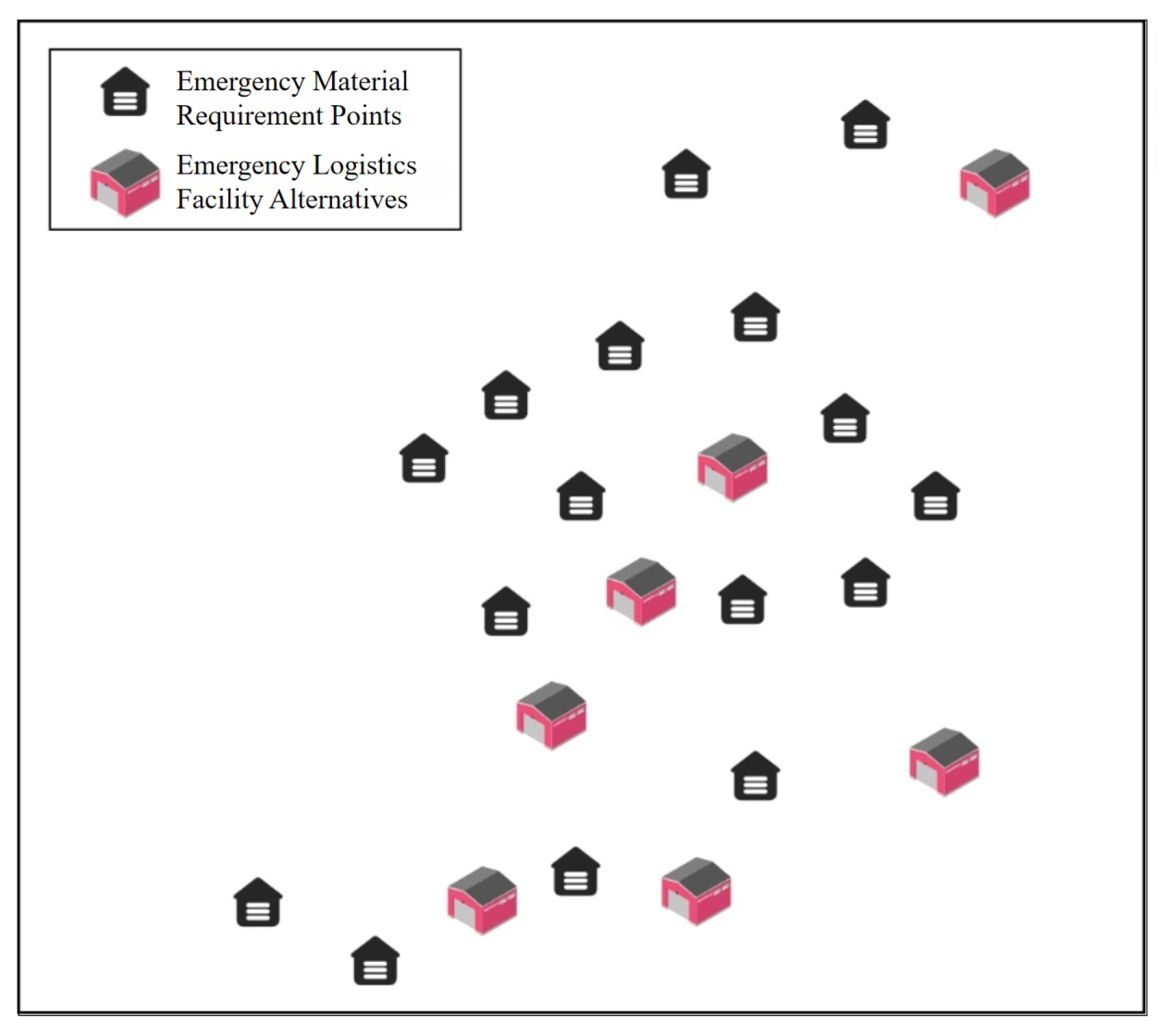
Allocation and scheduling rules: It is assumed that each emergency logistics facility can provide materials and dispatch human resources to multiple emergency logistics demand points, as shown in Figure 1(1). Each emergency supply–demand point can be serviced by multiple emergency logistics facilities, as shown in Figure 1(2), allowing for a flexible and robust supply chain.

6.

Demand relationship: The demand for supplies at emergency supply points is proportional to the demand for human resources. If a place has a large demand for supplies, it may be densely populated or severely affected by a disaster. Therefore, it will have more injured people and more affected groups, so it needs more emergency rescue human resources.

The specific schematic diagram of the model is shown in Figure 1. The various parameters required in the model, including sets, parameters, decision variables, etc., are as follows:

Sets and subscripts:

• I: The set of emergency supply–demand points, $i\in I$;
• J: The set of emergency logistics alternative facility points, $j\in J$;
• K: The set of emergency logistics rescue scenarios, $k\in K$.

Parameters:

• $c_t$: Unit transportation cost between emergency supply–demand point i and emergency logistics facility j;
• $d_{ij}$: Transportation distance between emergency supply–demand point i and emergency logistics facility j;
• $d_{\max }$: Maximum service distance of emergency logistics facility;
• $f_j$: Construction cost of emergency logistics facility j;
• $c_u$: Storage cost of unit emergency supplies during pre-disaster emergency supplies reserve;
• $v_j$: Storage capacity limit of emergency logistics facility;
• $p{c}_j$: The cost of dispatching a unit of professional emergency rescue human resources;
• $s{c}_j$: The cost of dispatching a unit of social emergency rescue human resources;
• $g{c}_j$: The cost of dispatching a unit of grassroots emergency rescue human resources;
• $D_i$: Demand quantity of emergency supply–demand point i;
• V: Speed of emergency supply transport vehicle;
• $T_{ij}$: Transportation time between emergency supply–demand point i and emergency logistics facility j;
• ${\zeta }_1,{\zeta }_2,{\zeta }_3$: The ratio coefficient of the demand for one unit of emergency supplies to the demand for one unit of professional/social/grassroots emergency rescue human resources at the demand point;
• $\sigma$: Road congestion coefficient;
• ${\sigma }_k$: Road congestion coefficient under scenario k;
• P: Maximum number of emergency logistics facilities to be built.

Decision variables:

• $y_j$: 0–1 binary variable; if emergency logistics facility j is selected, the value is 1, otherwise it is 0;
• $x_{ij}$: 0–1 binary variable; if emergency logistics facility j provides supplies to demand point i, the value is 1, otherwise it is 0;
• $x_{ijk}$: 0–1 binary variable, under scenario K; if the emergency logistics facility j provides supplies to the demand point i, the value is 1, otherwise it is 0;
• $u_j$: The quantity of emergency supplies stored at emergency logistics facility j;
• $q_{ij}$: The amount of supplies allocated by emergency logistics facility j to emergency supply–demand point i;
• $q_{ijk}$: The amount of material distributed by emergency logistics facility j to emergency material demand point i under scenario k;
• $p{r}_{ij}$: The number of professional emergency rescue human resources dispatched from emergency logistics facility j to demand point i;
• $s{r}_{ij}$: The number of social emergency rescue human resources dispatched from emergency logistics facility j to demand point i;
• $g{r}_{ij}$: The number of grassroots emergency rescue human resources dispatched from emergency logistics facility j to demand point i;
• $p{r}_{ijk}$: The number of professional emergency rescue human resources dispatched from emergency logistics facility j to demand point i under scenario K;
• $s{r}_{ijk}$: The number of grassroots emergency rescue human resources dispatched from emergency logistics facility j to demand point i under scenario K;
• $g{r}_{ijk}$: The number of grassroots emergency rescue human resources dispatched from emergency logistics facility j to demand point i under scenario K.

3.2. Basic Model

Based on the parameter settings above, this section first develops a mixed-integer programming (MIP) model based on the minimum locating and dispatching cost. The objective function is to minimize the total locating and dispatching cost, which includes construction cost, storage cost, and transportation costs:

$$min{Z}_1=\sum _{j\in J}{f}_j{y}_j+\sum _{j\in J}{c}_u{u}_j+\sum _{i\in I}\sum _{j\in J}{c}_t{x}_{ij}{q}_{ij}{d}_{ij}+\sum _{i\in I}\sum _{j\in J}(p{c}_{j}p{r}_{ij}+s{c}_{j}s{r}_{ij}+g{c}_{j}g{r}_{ij})$$

(1)

$$s.t.\sum _{i=1}^I{q}_{ij}\le u_j\le v_j,\forall i\in I,\forall j\in J$$

(2)

$$q_{ij}\le M\times x_{ij},\forall i\in I,\forall j\in J$$

(3)

$$d_{ij}{x}_{ij}\le d_{max},\forall i\in I,\forall j\in J$$

(4)

$$D_i\le \sum _{j\in J}{q}_{ij},\forall i\in I$$

(5)

$$\sum _{i\in I}p{r}_{ij}\le y_{j}M,\forall j\in J$$

(6)

$$\sum _{i\in I}s{r}_{ij}\le y_{j}M,\forall j\in J$$

(7)

$$\sum _{i\in I}g{r}_{ij}\le y_{j}M,\forall j\in J$$

(8)

$$D_i\le {\zeta }_1\sum _{j\in J}p{r}_{ij},\forall i\in I$$

(9)

$$D_i\le {\zeta }_2\sum _{j\in J}s{r}_{ij},\forall i\in I$$

(10)

$$D_i\le {\zeta }_3\sum _{j\in J}g{r}_{ij},\forall i\in I$$

(11)

$$y_j\in \{0,1\},x_{ij}\in \{0,1\},\forall i\in I\forall j\in J$$

(12)

The objective function (1) aims to minimize the total cost of locating, comprising the emergency logistics facility’s construction, the emergency supply storage cost, and transport cost. Constraint (2) specifies that each emergency logistics facility’s delivered emergency supplies are restricted by its storage capacity, which should not exceed the maximum capacity limit of the facility. Constraint (3) specifies that the designated emergency logistics facility is exclusively responsible for material delivery. A constraint factor of M, which guarantees proper supply flow, is achieved by utilizing a large integer. Constraint (4) prohibits the distance between the emergency logistics facility and the demand point from surpassing the maximum service distance. Constraint (5) ensures that all demands can be met through material distribution and that material transportation is always non-negative. Constraints (6)–(8) indicate that human resource dispatch decisions cannot be made when emergency logistics facility j is not selected. Constraints (9)–(11) require that the human resource dispatch to demand point i must meet the demand volume. Constraint (12) states that facility point $y_j$ is a binary variable that is equal to 1 when facility j is selected and 0 otherwise. The binary material allocation decision variable $x_{ij}$ is equal to 1 when facility j allocates material to the demand point and 0 otherwise.

Emergency logistics facilities are not designed to generate profits; thus, their expenses are often restricted. This leads to a situation where facility location is limited in cases with limited facilities. The previous section introduced the coverage model, which addresses the maximum coverage problem by selecting P facilities from alternative locations J to serve the maximum number of demand points I or satisfy the maximum amount of demand. This section focuses on incorporating constraints into the decision-making process for logistics facility locating.

$$\sum _{j\in J}{y}_j\le P$$

(13)

where P represents the threshold established by the decision-maker to prevent the number of selected emergency logistics facilities from exceeding the upper limit specified.

Following an emergency event, the arrival of emergency supplies at the demand point is often significantly delayed. Prolonged waiting times not only impact the affected individuals’ mood, but also hinder post-disaster emergency response and recovery efforts. To reduce the effects of emergencies on impacted individuals, this paper focuses on minimizing total transportation time as the second objective function.

$$min{Z}_2=\sigma \sum _{I,J}{T}_{ij}{x}_{ij}$$

(14)

$$s.t.T_{ij}=\frac{d_{ij}}{V},V\ge 0,T_{ij}\ge 0$$

(15)

where $\sigma$ denotes the road congestion coefficient; the occurrence of extreme disasters will seriously affect the smoothness of the rescue road and accordingly affect the transportation time of emergency supplies. Therefore, this paper introduces the $\sigma$ parameter to enhance the realism of the model. Equation (17) represents the corresponding constraint of the objective function $Z_2$, i.e., the transportation time between the emergency logistics facility point J and the emergency logistics demand point I can be obtained by the ratio of distance and transportation speed.

Considering both objective functions $Z_1$ described above, the dual-objective emergency logistics facility location model is obtained as Equation (16):

$$minZ=min{Z}_1+min{Z}_2$$

(16)

It is evident from Model (16) that time and transportation costs conflict with each other. In an emergency logistics network system, increasing optional emergency facilities will inevitably result in a reduction in transportation time and vice versa, as the cost rises. The significance of transportation cost and transportation time varies in different conditions. Therefore, this study aims to unify the two objective functions and proposes $\lambda$ as the weight coefficient for the two objectives. The value of $\lambda$ ranges between 0 and 1, and adjusting its value can alter the inputs of transportation time, and locating and dispatching cost. Consequently, the transformed objective function Z is obtained.

$$\begin{array}{cc}\hfill minZ& =min\left[\lambda Z_1+(1-\lambda )Z_2\right]\hfill \\ \hfill & =\lambda \left(\sum _J{f}_j{y}_j+\sum _J{c}_u{u}_j+\sum _{I,J}{q}_{ij}{x}_{ij}{d}_{ij}{c}_t+\sum _{I,J}(p{c}_{j}p{r}_{ij}+s{c}_{j}s{r}_{ij}+g{c}_{j}g{r}_{ij})\right)\hfill \\ \hfill & +(1-\lambda )\sum _{I,J}{T}_{ij}{x}_{ij}\hfill \end{array}$$

(17)

Since objective function $Z_2$, measured in time units, is challenging to evaluate alongside objective function $Z_1$, which is based on locating and dispatching costs, this paper aims to establish a quantitative assessment for Equation (17). Additionally, we will use the percentage standardization method to remove any unit discrepancies in the objective function. Set $Z_1^{*}$ and $Z_2^{*}$ as the minimum values of the single objective of the objective functions $Z_1$ and $Z_2$. Furthermore, let $Z_1^T$ and $Z_2^T$ denote the transformed objective functions. Thus, the degree of affiliation function of the objective function may be expressed in the following manner.

$$Z_1^T=\frac{Z_1}{Z_1^{*}},Z_2^T=\frac{Z_2}{Z_2^{*}}$$

(18)

Substituting Equation (18) into Equation (17):

$$\begin{array}{cc}\hfill minZ& =min\lambda Z_1^T+(1-\lambda )Z_2^T\hfill \\ \hfill & =\lambda \frac{\left({\sum }_J{f}_j{y}_j+{\sum }_J{c}_u{u}_j+{\sum }_{I,J}{q}_{ij}{x}_{ij}{d}_{ij}{c}_t+{\sum }_{I,J}(p{c}_{j}p{r}_{ij}+s{c}_{j}s{r}_{ij}+g{c}_{j}g{r}_{ij})\right)}{Z_1^{*}}\hfill \\ \hfill & +(1-\lambda )\frac{{\sum }_{I,J}{T}_{ij}{x}_{ij}}{Z_2^{*}}\hfill \end{array}$$

(19)

The above model follows the Equations (2)–(13) and (15) mentioned earlier. Equation (19) is a MIP for locating emergency logistics facilities proposed in this section, which takes into account transportation costs and transportation time, and is transformed into a single-objective model by normalizing the time weights $\lambda$ and percentages. When $\lambda$ is set to 1, the model is equivalent to the single-objective model based on locating and dispatching cost. When $\lambda$ is 0, the model is equivalent to a single-objective model based on transportation time.

Property 1.

The MILP model constructed in this paper has feasible solutions.

Proof. 

The model is a MILP problem, which involves both continuous and binary variables. One way to prove the existence of feasible solutions for a MILP problem is to use the concept of relaxation. Relaxation means removing some of the constraints or variables from the original problem to make it easier to solve. For example, if we relax the binary constraints on $y_j$ and $x_{ij}$, we obtain a linear programming (LP) problem, which can be solved efficiently by standard methods. The feasible region of the LP relaxation is larger than or equal to the feasible region of the MILP problem. Therefore, if the LP relaxation has a feasible solution, then the MILP problem also has a feasible solution. This is called the sufficiency condition for feasibility. Then, through Theorems 4.1 and 2.1 [44,45], it can be clearly concluded that the MILP model constructed in this article has feasible solutions. □

Property 2.

If the continuous variables are bounded, the MILP model constructed in this paper has an optimal solution.

Proof. 

According to Theorem 1 as cited in [46], if the continuous variables within a model are bounded, and both the objective function and constraints are continuous, it results in the feasible region being a compact set. In such a scenario, the objective function is guaranteed to attain its optimal value within this set. Given that the continuous variables in our model are indeed bounded, we can infer that the mixed-integer programming model we have constructed will have an optimal solution. □

If there is only one point in the feasible domain, then the solution of the MILP model constructed in this paper is unique. However, in our model, the decision variables $x_{ij}$ and $y_j$ are binary, which means they can take on either of two values: 0 or 1. This inherently introduces multiple combinations of variable assignments that could potentially satisfy the constraints and optimize the objective function. In a MILP problem, the feasible region is a discrete set and there can be multiple points (solutions) in this set that give the same optimal value of the objective function. This is especially true when the objective function is linear, as is the case in MILP. In such cases, any point on the line segment connecting two optimal solutions is also optimal, leading to an infinite number of optimal solutions. Let us consider a simple scenario where there are two facilities ($j=2$) and two customers ($i=2$). Even in this simplified case, there are $2^{2\ast 2}=16$ possible combinations for the binary decision variable $x_{ij}$ alone. Each of these combinations could potentially be a feasible solution, depending on the specific parameters and constraints of the problem. Moreover, the objective function in our model is a linear combination of the decision variables. In linear programming, if the objective function is parallel to one of the constraints at the optimal point, multiple optimal solutions can exist. This is because moving along the constraint does not change the value of the objective function. So, we cannot prove the uniqueness of the solution for the MILP model constructed in this article. Just as Huang et al. [47] proved in their paper that MILP is an NP hard problem with multiple solutions, the original problem needs to be divided into several subproblems for solving.

4. Stochastic Programming Model

This section considers a TSP model for emergency logistics facility locations with environmental uncertainty. In the first stage, the construction and storage costs of the emergency logistics facility are considered. As a decision-maker, one needs to first decide on whether to place a location at a J point and the amount of emergency supplies to be stored at that facility point. Decisions at this stage, the strategic level, are independent of uncertainty, and incur the same costs regardless of the probability of an event occurring and how demand changes. The first stage of the problem can then be represented separately as Equation (20).

$$minZ=\sum _{j\in J}{f}_j{y}_j+\sum _{j\in J}{c}_u{u}_j$$

(20)

After confirming the objective function of the first stage, consider the problem of the second stage. The second stage is called the practical layer, which can also be understood as the pursuit and compensation for the first-stage problem. This section takes Q as the objective function, representing transportation costs and transportation time. In actual emergency material relief, the uncertainty of material demand and road conditions will lead to instability in transportation costs and transportation time. Corresponding to the model, that is, the change in $q_{ij}$ is related to $D_i$. On the other hand, this article adds a road congestion coefficient ${\sigma }_k$ to the transportation time and changes the transportation time under different scenarios by taking different values of ${\sigma }_k$, to simulate the real rescue road situation. In summary, considering transportation costs and transportation time separately in the second stage can effectively avoid mutual influence with the decision-making of the first stage, specifically expressed as Equation (21):

$$\begin{array}{cc}\hfill Q_k(x,q,pr,sr,gr,\sigma )& =\lambda \left(c_t{x}_{ijk}{q}_{ijk}{d}_{ij}+p{c}_{j}p{r}_{ijk}+s{c}_{j}s{r}_{ijk}+g{c}_{j}g{r}_{ijk}\right)\hfill \\ \hfill & +(1-\lambda ){\sigma }_k{T}_{ij}{x}_{ijk}\hfill \end{array}$$

(21)

Because we need to calculate the expectation of the objective function in the second stage, Equation (21) is further expanded into an extended form of a scenario-based stochastic programming model. Considering the probability of different scenarios K occurring as $P_K,P_K\in P$, the expected cost of the second stage can be expressed as Equation (22):

$$\begin{array}{cc}\hfill & E_K\left[Q(x,q,pr,sr,gr,\sigma )\right]\hfill \\ \hfill & =\sum _{i\in I,j\in J,k\in K}{P}_k{Q}_k(x,q,pr,sr,gr,\sigma )\hfill \\ \hfill & =\sum _{i\in I,j\in J,k\in K}{P}_k\left[\lambda \left(c_t{x}_{ijk}{q}_{ijk}{d}_{ij}+p{c}_{j}p{r}_{ijk}+s{c}_{j}s{r}_{ijk}+g{c}_{j}g{r}_{ijk}\right)\right.\hfill \\ \hfill & \left.+(1-\lambda ){\sigma }_k{T}_{ij}{x}_{ijk}\right]\hfill \\ \hfill & \mathrm{s}.\mathrm{t}.\sum _{k\in K}{P}_k=1\hfill \end{array}$$

(22)

Therefore, the TSP model for emergency logistics facility location established in this paper can be expressed as Equation (23):

$$\begin{array}{cc}\hfill & minZ=\sum _{j\in J}{f}_j{y}_j+\sum _{j\in J}{c}_u{u}_j+E_K\left[Q(x,q,pr,sr,gr,\sigma )\right]\hfill \end{array}$$

(23)

The above model follows the Equations (2)–(13), (15) and (22) mentioned earlier. Similarly to the dimension conversion method in Section 3, Equation (23) can be expanded and transformed into Equation (24):

$$\begin{array}{cc}\hfill minZ& =\lambda \frac{{\sum }_{j\in J}{f}_j{y}_j+{\sum }_{j\in J}{c}_u{u}_j}{Z_1^{*}}\hfill \\ \hfill & +E_K\left[\lambda \frac{{\sum }_{i\in I,j\in J}(x_{ijk}{q}_{ijk}{d}_{ij}{c}_t+p{c}_{j}p{r}_{ijk}+s{c}_{j}s{r}_{ijk}+g{c}_{j}g{r}_{ijk})}{Z_1^{*}}\right.\hfill \\ \hfill & \left.+(1-\lambda )\frac{{\sum }_{i\in I,j\in J}{\sigma }_k{T}_{ij}{x}_{ijk}}{Z_2^{*}}\right]\hfill \end{array}$$

(24)

where $Z_1^{*}$ and $Z_2^{*}$ are, respectively, the minimum values of transportation costs and transportation time in the MIP model proposed in Section 3.

TSP Model for Emergency Logistics Facility Location Based on Risk Preference

To effectively measure the extreme tail risk in the emergency logistics facility location studied in this paper, CVaR is introduced to further optimize the TSP model proposed in Section 3. Since the uncertainty of demand and road conditions is related to the second stage, this paper changes the expected value of the second stage to a target function based on CVaR:

$${CVaR}_{\alpha }\left(Q(x,q,pr,sr,gr,\sigma )\right)=min\left\{\eta +{(1-\alpha )}^{-1}E\left[{(Q(x,q,pr,sr,gr,\sigma )-\eta )}_{+}\right]\right\}$$

(25)

where $\eta$ is the threshold that the expected loss does not exceed and

$${[Q(x,q,pr,sr,gr,\sigma )-\eta ]}_{+}=\underset{n\in R}{max}\{0,Q(x,q,pr,sr,gr,\sigma )-\eta \}$$

(26)

Notice that the function of cost and time exists in $CVa{R}_{\alpha }\left(Q(x,q,\sigma )\right)$ at the same time. For convenience of calculation, the following transformation is made to Equation (25):

$$\begin{array}{cc}\hfill & {CVaR}_{\alpha }\left(Q(x,q,pr,sr,gr,\sigma )\right)\hfill \\ \hfill & ={CVaR}_{\alpha }\left[\lambda \left(c_t{x}_{ijk}{q}_{ijk}{d}_{ij}+p{c}_{j}p{r}_{ijk}+s{c}_{j}s{r}_{ijk}+g{c}_{j}g{r}_{ijk}\right)\right]+{CVaR}_{\alpha }\left[(1-\lambda ){\sigma }_k{T}_{ij}{x}_{ijk}\right]\hfill \\ \hfill & =\lambda {CVaR}_{\alpha }\left(c_t{x}_{ijk}{q}_{ijk}{d}_{ij}+p{c}_{j}p{r}_{ijk}+s{c}_{j}s{r}_{ijk}+g{c}_{j}g{r}_{ijk}\right)+(1-\lambda )CVa{R}_{\alpha }\left({\sigma }_k{T}_{ij}{x}_{ijk}\right)\hfill \\ \hfill & =min\lambda \left\{{\eta }_1+{(1-\alpha )}^{-1}E\left[{\left(c_t{x}_{ijk}{q}_{ijk}{d}_{ij}+p{c}_{j}p{r}_{ijk}+s{c}_{j}s{r}_{ijk}+g{c}_{j}g{r}_{ijk}-{\eta }_1\right)}_{+}\right]\right\}\hfill \\ \hfill & +(1-\lambda )\left\{{\eta }_2+{(1-\alpha )}^{-1}E\left[{\left({\sigma }_k{T}_{ij}{x}_{ijk}-{\eta }_2\right)}_{+}\right]\right\}\hfill \end{array}$$

(27)

where $\alpha$ is the same risk level, and ${\eta }_1,{\eta }_2$ are, respectively, the expected transportation cost and transportation time determined by the decision-maker. To prove the effective range of $\eta$, the following proposition is proposed:

Proposition 1.

The range of expected loss value η is $\left[0,{\eta }_{\max }\right]$, where ${\eta }_{\max }$ is the upper limit defined by the decision-maker. That is

$$\eta \in \left[0,{\eta }_{max}\right]$$

(28)

Proof of Proposition 1 .

According to the CVaR formula proposed by Rockafellar and Uryasev [48]:

$${CVaR}_{\alpha }\left(X\right)=\underset{\eta \in R}{min}\left\{\eta +{(1-\alpha )}^{-1}E\left[{(X-\eta )}_{+}\right]\right\}$$

(29)

When $\eta \le 0$, we can obtain:

$$\eta +{(1-\alpha )}^{-1}E\left[{(X-\eta )}_{+}\right]=\left(1-{(1-\alpha )}^{-1}\right)\eta +{(1-\alpha )}^{-1}E\left[X\right]$$

(30)

Since $\alpha \in [0,1]$, so at this time $\left(1-{(1-\alpha )}^{-1}\right)<0$, Equation (30) tends to negative infinity as $\eta$ changes. When $\eta \ge {\eta }_{\max }$, we can obtain:

$$\eta +{(1-\alpha )}^{-1}E\left[{(X-\eta )}_{+}\right]=\eta$$

(31)

It is easy to know that, at this time ${(1-\alpha )}^{-1}E\left[{(X-\eta )}_{+}\right]=0$, Equation (31) tends to positive infinity as $\eta$ changes. Considering the convexity of the function, the effective range of $\eta$ is $\left[0,{\eta }_{\max }\right]$. In summary, the risk preference two-stage stochastic programming (RP-TSP) model for emergency logistics facility location based on risk preference established in this paper can be written as follows:

$$\begin{array}{cc}\hfill & minZ=\sum _{j\in J}{f}_j{y}_j+\sum _{j\in J}{c}_u{u}_j+{CVaR}_{\alpha }\left(Q(x,q,pr,sr,gr,\sigma )\right)\hfill \end{array}$$

(32)

The above model follows the Equations (2)–(13), (15), (27) and (28) mentioned earlier. The dimension handling method of Equation (32) is the same as that of Equation (24) and it will not be repeated here. □

5. Robust Optimization Model

In this section, we use the method of robust optimization for emergency logistics facility location modeling. First, we will establish a robust model based on the box uncertainty set and then establish a robust model based on the polyhedron uncertainty set with adjustable robust conservatism. Since the robust model of Ben-Tal and Nemirovski [28] is a second-order cone model and has not been widely applied, it is not considered in this paper.

5.1. Robust Model for Emergency Logistics Facility Location Based on Box Uncertainty Set

First, according to Soyster’s [49] robust model, we establish a robust model based on the box uncertainty set. Suppose $a_m$ is the mth row vector of the uncertainty parameter matrix A, where $N_m$ is the set of the uncertain part $a_{mn}$ in the mth row of matrix A. The uncertainty parameter $a_{mn}$ can vary in the interval $\left[{\overline{a}}_{mn}-{\widehat{a}}_{mn},{\overline{a}}_{mn}+{\widehat{a}}_{mn}\right]$, where ${\overline{a}}_{mn}$ is the nominal value, ${\widehat{a}}_{mn}$ is the perturbation value, and ${\widehat{a}}_{mn}\ge 0$. Referring to the Soyster robust model, the uncertainty set of demand $D_i$ in constraint (4) can be expressed as follows:

$$\begin{array}{cc}\hfill max\left\{D_i\right\}& =max\left\{\sum _{n\in N_m}{a}_{mn}{D}_i+\sum _{n\notin N_m}{a}_{mn}{D}_i\right\}\hfill \\ \hfill & =max\left\{\sum _{n\in N_m}{a}_{mn}{D}_i+\sum _{n\notin N_m}{\overline{a}}_{mn}{D}_i\right\}\hfill \\ \hfill & =max\left\{\sum _{n\in N_m}{a}_{mn}{D}_i+\sum _{n\in N_m}{\overline{a}}_{mn}{D}_i-\sum _{n\in N_m}{\overline{a}}_{mn}{D}_i+\sum _{n\notin N_m}{\overline{a}}_{mn}{D}_i\right\}\hfill \\ \hfill & =max\left\{\sum _n{\overline{a}}_{mn}{D}_i+\sum _{n\in N_m}\left(a_{mn}-{\overline{a}}_{mn}\right)D_i\right\}=\sum _n{\overline{a}}_{mn}{D}_i+\sum _{n\in N_m}\left|{\widehat{a}}_{mn}{D}_i\right|\hfill \end{array}$$

(33)

Then, constraint (5) and (9)–(11) can be rewritten as follows:

$$\sum _n{\overline{a}}_{mn}{D}_i+\sum _{n\in N_m}\left|{\widehat{a}}_{mn}{D}_i\right|\le \sum _{j\in J}{q}_{ij},\forall i\in I$$

(34)

$$\sum _n{\overline{a}}_{mn}{D}_i+\sum _{n\in N_m}\left|{\widehat{a}}_{mn}{D}_i\right|\le {\zeta }_1\sum _{j\in J}p{r}_{ij},\forall i\in I$$

(35)

$$\sum _n{\overline{a}}_{mn}{D}_i+\sum _{n\in N_m}\left|{\widehat{a}}_{mn}{D}_i\right|\le {\zeta }_2\sum _{j\in J}s{r}_{ij},\forall i\in I$$

(36)

$$\sum _n{\overline{a}}_{mn}{D}_i+\sum _{n\in N_m}\left|{\widehat{a}}_{mn}{D}_i\right|\le {\zeta }_3\sum _{j\in J}g{r}_{ij},\forall i\in I$$

(37)

Introduce variable $H_i$ to eliminate the absolute value in Equations (34)–(37):

$$\begin{array}{cc}\hfill & \sum _n{\overline{a}}_{mn}{D}_i+\sum _{n\in N_m}{\widehat{a}}_{mn}{H}_i\le \sum _{j\in J}{q}_{ij},\forall i\in I\hfill \\ \hfill & \sum _n{\overline{a}}_{mn}{D}_i+\sum _{n\in N_m}{\widehat{a}}_{mn}{H}_i\le {\zeta }_1\sum _{j\in J}p{r}_{ij},\forall i\in I\hfill \\ \hfill & \sum _n{\overline{a}}_{mn}{D}_i+\sum _{n\in N_m}{\widehat{a}}_{mn}{H}_i\le {\zeta }_2\sum _{j\in J}s{r}_{ij},\forall i\in I\hfill \\ \hfill & \sum _n{\overline{a}}_{mn}{D}_i+\sum _{n\in N_m}{\widehat{a}}_{mn}{H}_i\le {\zeta }_3\sum _{j\in J}g{r}_{ij},\forall i\in I\hfill \\ \hfill & \mathrm{s}.\mathrm{t}.-H_i\le D_i\le H_i\hfill \\ \hfill & H_i\ge 0\hfill \end{array}$$

(38)

Then, the original model is equivalent to the following:

$$\begin{array}{cc}\hfill minZ& =\lambda \left(\sum _{j\in J}{f}_j{y}_j+\sum _{j\in J}{c}_u{u}_j+\sum _{i\in I,j\in J}{q}_{ij}{x}_{ij}{d}_{ij}{c}_t+\sum _{I,J}(p{c}_{j}p{r}_{ij}+s{c}_{j}s{r}_{ij}+g{c}_{j}g{r}_{ij})\right)\hfill \\ \hfill & +(1-\lambda )\sigma \sum _{i\in I,j\in J}{T}_{ij}{x}_{ij}\hfill \end{array}$$

(39)

The above model follows the Equations (2)–(4), (6)–(8), (12), (13), (15) and (38) mentioned earlier. Model (39) is the robust optimization model based on the box uncertainty set (RO-B) for the emergency logistics facility location set up in this paper. The dimension handling method of this model is the same as that of Equation (24) and it will not be repeated here.

5.2. Robust Model for Emergency Logistics Facility Location Based on Polyhedral Uncertainty Set

To further consider the uncertainty of demand $D_i$, this section continues to refer to the robust model proposed by Bertsimas and Sim for modeling.

Assume ${\overline{D}}_i$ is the nominal value of $D_i$ and ${\widehat{D}}_i$ is the perturbation value of demand; then, $D_i$ changes in the interval $\left[{\overline{D}}_i-{\widehat{D}}_i,{\overline{D}}_i+{\widehat{D}}_i\right]$. Similarly, set up the uncertainty parameter matrix $A(m\times n)$ and introduce the parameter $\Gamma$ of perturbation value to adjust the conservatism of the model, where $a_{mn}\le {\Gamma }_m$. Let a part of $D_i$ in the model fluctuate, where $⌊{\Gamma }_m⌋$ changes in $\left[{\overline{D}}_i-{\widehat{D}}_i,{\overline{D}}_i+{\widehat{D}}_i\right]$ (where $⌊{\Gamma }_m⌋$ represents the maximum integer not exceeding ${\Gamma }_m$), 1 changes in $\left[{\overline{D}}_i-{\widehat{D}}_i\left({\Gamma }_m-⌊{\Gamma }_m⌋\right),{\overline{D}}_i+{\widehat{D}}_i\left({\Gamma }_m-⌊{\Gamma }_m⌋\right)\right]$, and the rest of $D_i$ does not change, and does not specify the specific change in ${\Gamma }_m$ uncertainty parameters. Therefore, the uncertainty parameter $D_i$ in the model can be expressed as follows:

$$D_i=\sum _n{a}_{mn}{\overline{D}}_i+G\left(D_i,{\Gamma }_m\right)$$

(40)

where

$$\begin{array}{cc}\hfill & G\left(D_i,{\Gamma }_m\right)\hfill \\ \hfill & =\underset{\left\{S_m\cup \left\{t_m\right\}\left|S_m\subseteq N_m,\right|S_m\mid \in {\Gamma }_m,t_m\in N_m\setminus S_m\right\}}{max}\left\{\sum _{n\in S_m}{\widehat{a}}_{mn}\left|D_i^{*}\right|+\left({\Gamma }_m-⌊{\Gamma }_m⌋\right){\widehat{a}}_{m{t}_m}\left|D_i^{*}\right|\right\}\hfill \end{array}$$

(41)

where the subscript S in the objective function is the set of points where demand fluctuation occurs. When ${\Gamma }_m$ is 0, Equation (40) degenerates into a nominal problem. When ${\Gamma }_m=\left|N_m\right|$, Equation (40) is equivalent to the robust model proposed by Soyster. Therefore, by changing ${\Gamma }_m$ in the interval $\left[0,\left|N_m\right|\right]$, the conservatism of the model can be effectively controlled. It is not difficult to see that Equation (40) is a nonlinear problem, and it will be transformed into a linear problem for the solution next. When ${\Gamma }_m$ is an integer:

$$G\left(D_i,{\Gamma }_m\right)=\underset{S_m\subseteq N_m,S_m\in {\Gamma }_m}{max}\sum _{n\in N_m}{\widehat{a}}_{mn}\left|D_i^{*}\right|$$

(42)

Introduce auxiliary variable $z_{mn}$ to eliminate the constraint of subscript S in the objective function:

$$\begin{array}{cc}\hfill & G\left(D_i,{\Gamma }_m\right)=max\sum _{n\in N_m}{\widehat{a}}_{mn}\left|D_i^{*}\right|z_{mn}\hfill \\ \hfill & \mathrm{s}.\mathrm{t}.\sum _{n\in N_m}{z}_{mn}\le {\Gamma }_m\hfill \\ \hfill & 0\le z_{mn}\le 1\forall n\in N_m\hfill \end{array}$$

(43)

The dual problem of model (43) is the following:

$$\begin{array}{cc}\hfill & min\sum _{n\in N_m}{p}_{mn}+z_m{\Gamma }_m\hfill \\ \hfill & \mathrm{s}.\mathrm{t}.z_m+p_{mn}\ge {\widehat{a}}_{mn}{D}_i\forall m,n\in N_m\hfill \\ \hfill & p_{mn}\ge 0\forall n\in N_m\hfill \\ \hfill & z_m\ge 0\forall m\hfill \end{array}$$

(44)

where p is the auxiliary variable of the dual problem. Therefore, constraints (34)–(37) in the model can be rewritten as follows:

$$\begin{array}{cc}\hfill & \sum _n{a}_{mn}{\overline{D}}_i+\sum _{n\in N_m}{p}_{mn}+z_m{\Gamma }_m\le \sum _{j\in J}{q}_{ij},\forall i\in I\hfill \\ \hfill & \sum _n{a}_{mn}{\overline{D}}_i+\sum _{n\in N_m}{p}_{mn}+z_m{\Gamma }_m\le {\zeta }_1\sum _{j\in J}p{r}_{ij},\forall i\in I\hfill \\ \hfill & \sum _n{a}_{mn}{\overline{D}}_i+\sum _{n\in N_m}{p}_{mn}+z_m{\Gamma }_m\le {\zeta }_1\sum _{j\in J}s{r}_{ij},\forall i\in I\hfill \\ \hfill & \sum _n{a}_{mn}{\overline{D}}_i+\sum _{n\in N_m}{p}_{mn}+z_m{\Gamma }_m\le {\zeta }_1\sum _{j\in J}g{r}_{ij},\forall i\in I\hfill \\ \hfill & z_m+p_{mn}\ge {\widehat{a}}_{mn}{D}_i\forall m,n\in N_m\hfill \\ \hfill & p_{mn}\ge 0\forall n\in N_m\hfill \\ \hfill & z_m\ge 0\forall m\hfill \end{array}$$

(45)

Then, the original model is equivalent to the following:

$$\begin{array}{cc}\hfill & minZ=\lambda \left(\sum _{j\in J}{f}_j{y}_j+\sum _{j\in J}{c}_u{u}_j+\sum _{i\in I,j\in J}{q}_{ij}{x}_{ij}{d}_{ij}{c}_t\right)+(1-\lambda )\sigma \sum _{i\in I,j\in J}{T}_{ij}{x}_{ij}\hfill \end{array}$$

(46)

The above model follows the Equations (2)–(4), (6)–(8), (12), (13), (15) and (45) mentioned earlier. The model of Equation (46) is the robust optimization model based on the polyhedral uncertainty set (RO-P) for the emergency logistics facility location set up in this paper. The dimension handling method of this model is the same as that of Equation (24) and it will not be repeated here.

6. Numerical Analysis

6.1. Numerical Example

There are many application scenarios for the locating of emergency logistics facilities, including natural disasters such as earthquakes and various public health events. In this paper, we have selected the more frequent earthquakes in China’s southwestern region of Sichuan Province for research. Regarding the historical data of the Wenchuan earthquake and the map of Sichuan Province, this paper selects sixteen counties and cities that were severely affected by the earthquake as the emergency material demand points for modeling and analysis, and their geographic locations are mainly concentrated in the northwest of the Sichuan Basin along the Longmen Mountain Range. The sixteen counties and cities are Wenchuan County, Beichuan County, Mianzhu City, Qingchuan County, Mao County, Dujiangyan City, Pingwu County, Pengzhou City, Santai County, Lezhi County, Zhongjiang County, Renshou County, Zitong County, Yanting County, Hongya County, and Ya’an City. Figure 2 represents the geographic locations of the study cases in this section and the approximate distribution of the locations of the demand points.

6.1.1. Pre-Locating of Emergency Logistics Facilities

This section discusses the criteria and factors necessary for the placement of an emergency logistics facility, as presented in this paper’s case study. Unlike traditional logistics, emergency logistics, characterized by suddenness, uncertainty, nonroutine activities, unconventionality, and a weak economy, requires a more rigorous process for facility locating. The selection of locations for these facilities must be objective, incorporating historical data, objective factors, and scientific models to ensure a comprehensive and reasonable choice. Emergency logistics prioritizes people and aims to reduce the impact of disasters on individuals. It adopts a comprehensive approach to disaster relief to minimize community devastation. As per the relevant literature [50,51,52], the analysis of emergency logistics facilities should focus on location factors. This paper considers factors such as population density, service area, transportation accessibility, spatial capacity, and economic costs for pre-locating emergency logistics facilities. In the context of Sichuan Province, seven cities—Chengdu, Deyang, Mianyang, Guangyuan, Ziyang, Meishan, and Suining—were selected as alternative locations for the facilities. These prefecture-level cities each have a population of over 1 million and are within 500 km of the hypothetical demand point for emergency supplies. Additionally, these locations offer good transportation conditions with multiple highways and railroads ensuring timely response and service to affected areas. Figure 3 shows the abstract model map of the alternative emergency logistics facilities and demand points.

6.1.2. Parameters of Model

The maximum capacity, unit storage cost, and construction cost of each facility option are shown in

Table 2. Overview of emergency logistics facilities.

Alternative	${\mathit{f}}_{\mathit{j}}$	${\mathit{c}}_{\mathit{u}}$	${\mathit{v}}_{\mathit{j}}$	${\mathit{pc}}_{\mathit{j}}$	${\mathit{sc}}_{\mathit{j}}$	${\mathit{gc}}_{\mathit{j}}$
Locations	(USD 10,000)	(USD 10,000/10,000 Units)	(10,000 Units)	(USD 10,000/10,000 Units)	(USD 10,000/10,000 Units)	(USD 10,000/10,000 Units)
Chengdu	240	0.3	80	260	180	40
Deyang	180	0.25	60	340	230	50
Mianyang	180	0.25	60	400	260	65
Guangyuan	180	0.25	60	480	310	80
Meishan	150	0.2	50	340	230	50
Ziyang	150	0.2	50	340	230	50
Suining	150	0.2	50	400	260	65

. The capacity, storage cost, and construction cost of the emergency logistics facilities are referenced to the ‘Standards for the Construction of Disaster Relief Material Reserve Depots’ issued by the Ministry of Civil Affairs in 2009, as well as the local development level of the city. We rank the scheduling costs of three types of emergency rescue human resources based on the number of human resources and the difficulty of mobilization: professional > social > grassroots, and provide corresponding parameters in the table based on statistical data.

The distance between each emergency logistics facility alternative point and each emergency material demand point is calculated concerning the navigation route in Google Maps, and the specific data are shown in

Table 3. Distances from demand points to facility options (kilometers).

Alternative Locations	Chengdu	Deyang	Mianyang	Guangyuan	Meishan	Ziyang	Suining
Wenchuan County	144	162	198	328	202	225	297
Beichuan County	215	134	92	231	223	207	187
Mianzhu	116	35	60	221	180	180	185
Qingchuan County	300	218	174	92	389	353	313
Mao County	183	114	122	288	242	256	270
Dujiangyan	71	105	123	290	130	169	226
Pingwu County	293	212	160	167	360	347	302
Pengzhou	69	74	95	261	135	140	195
Santai County	138	106	72	222	207	160	99
Lezhi County	115	150	185	332	141	58	83
Zhongjiang County	97	39	59	235	165	120	141
Renshou County	78	152	200	367	34	65	179
Zitong County	201	122	60	150	268	258	194
Yanting County	174	135	126	222	243	196	94
Hongya County	123	208	255	438	63	139	253
Ya’an City	131	210	248	421	101	177	294

. Considering factors such as road conditions, safety considerations, vehicle capabilities, efficiency, and timeliness, the disaster area is mostly mountainous, and the road conditions are poor and affected by the earthquake, so we set the unit transportation speed in emergency logistics to 40 km/h. The ratio of distance and speed can be obtained from the time between the alternative points of each emergency logistics facility and the demand points of each emergency material, and the specific data are shown in

Table 4. Demand point to facility options (h).

Alternative Locations	Chengdu	Deyang	Mianyang	Guangyuan	Meishan	Ziyang	Suining
Wenchuan County	3.6	4.1	5	8.2	5.1	5.6	7.4
Beichuan County	5.4	3.4	2.3	5.8	5.6	5.2	4.7
Mianzhu	2.9	0.9	1.5	5.5	4.5	4.5	4.6
Qingchuan County	7.5	5.5	4.4	2.3	9.7	8.8	7.8
Mao County	4.6	2.9	3.1	7.2	6.1	6.4	6.8
Dujiangyan	1.8	2.6	3.1	7.3	3.3	4.2	5.7
Pingwu County	7.3	5.3	4	4.2	9	8.7	7.6
Pengzhou	1.7	1.9	2.4	6.5	3.4	3.5	4.9
Santai County	3.5	2.7	1.8	5.6	5.2	4	2.5
Lezhi County	2.9	3.8	4.6	8.3	3.5	1.5	2.1
Zhongjiang County	2.4	1	1.5	5.9	4.1	3	3.5
Renshou County	2	3.8	5	9.2	0.9	1.6	4.5
Zitong County	5	3.1	1.5	3.8	6.7	6.5	4.9
Yanting County	4.4	3.4	3.2	5.6	6.1	4.9	2.4
Hongya County	3.1	5.2	6.4	11	1.6	3.5	6.3
Ya’an City	3.3	5.3	6.2	10.5	2.5	4.4	7.4

.

The demand for materials in each city and county is mainly based on the population statistics in the 2021 Statistical Yearbook of Sichuan Province, as shown in

Table 5. Emergency material requirements by point of requirement.

Cities/Towns	Demand	Cities/Towns	Demand
	(10,000 Units)		(10,000 Units)
Wenchuan County	8	Santai County	20
Beichuan County	10	Lezhi County	10
Mianzhu	20	Zhongjiang County	20
Qingchuan County	8	Renshou County	20
Mao County	10	Zitong County	8
Dujiangyan	25	Yanting County	10
Pingwu County	10	Hongya County	12
Pengzhou	15	Ya’an City	20

. The other main parameters involved in the case background are as follows: the transportation cost is USD 0.0028 million/unit/km and the upper limit of facilities P is 7. The road congestion factor $\sigma$ for the defined environment in Section 6.2 is set to 1. To enable emergency supplies to serve the affected area in time, the maximum service distance of emergency logistics facilities $d_{max}$ is set to 300 km.

Given the intricacy and significant computational demands of the proposed model, this article utilizes the Gurobi solver to compile and solve the model. The solver is executed on a computer with an Intel Core i7-11700K CPU @ 4.80GHz operating environment.

6.2. Analysis of Location Results in Defined Environments

6.2.1. Comparative Analysis of Single Target Results

In this section, the location results of the single-objective MIP will be solved to obtain the $Z_1^{*}$ and $Z_2^{*}$ required for magnitude processing. In the single-objective model based on locating and dispatching cost, Chengdu, Deyang, Mianyang, and Meishan are selected, with a total locating and dispatching cost of $Z_1$ of USD 1,640,100 and a total transportation time of $Z_2$ of 43.4 h. The distribution data on emergency supplies are shown in

Table 6. Single-objective model results based on locating and dispatching costs (10,000 units).

Alternative Locations	Chengdu	Deyang	Mianyang	Meishan
Wenchuan County	8
Beichuan County			10
Mianzhu		20
Qingchuan County			8
Mao County		10
Dujiangyan	25
Pingwu County			10
Pengzhou	15
Santai County		6	14
Lezhi County	10
Zhongjiang County		20
Renshou County				20
Zitong County		8
Yanting County		10
Hongya County				12
Ya’an City	2			18

, and the utilization rate of each alternative location is 75%, 93.3%, 100%, and 100%, respectively.

The model is based on the transportation time of the location results of all alternative facilities selected, the total locating and dispatching cost $Z_1$ for USD 2.346 million, and the total transportation time $Z_2$ for 33.2 h. The distribution data of emergency supplies are shown in

Table 7. Single-objective modeling results based on transit time (10,000 units).

Alternative Locations	Chengdu	Deyang	Mianyang	Guangyuan	Meishan	Ziyang	Suining
Wenchuan County	8
Beichuan County			10
Mianzhu		20
Qingchuan County				8
Mao County		10
Dujiangyan	25
Pingwu County			10
Pengzhou	15
Santai County			20
Lezhi County						10
Zhongjiang County		20
Renshou County			8
Zitong County			10
Yanting County							10
Hongya County					12
Ya’an City	20

, and the facility utilization rate of each alternative location is calculated to be $85\%,83.3\%$, $80\%,13.3\%$, $64\%,20\%,20\%$, and $20\%$, respectively.

From the above results, the minimum values of $Z_1^{*}$ and $Z_2^{*}$ for the single-objective model are 11,714,800 and 33.2 h, respectively. Through the analysis of the above results, it can be found that, when the emergency logistics facility locating model is a single-objective model, the locating and dispatching cost, and transportation time can be reduced by 30.1% and 24.5%, respectively, compared with the relative situation, but, accordingly, it will also bring about a significant increase in the value of the other objective function. It is easy to find that, although the results in Table 7 minimize the emergency response time, the utilization rate of emergency logistics facilities is lower; some facilities have a utilization rate of even less than 20. Minimizing transportation time is certainly the first consideration in the decision of emergency logistics location but, due to the nonprofit nature of emergency logistics, the high cost of location and dispatching will often increase the economic burden of local governments. Therefore, the following section will further analyze the importance of the two objective functions of locating and dispatching cost, and transportation time in the context of this paper by changing the weight coefficients in the model.

6.2.2. Comparative Analysis of Dual Objective Results

In Section 3.2, the conflicting nature of locating and dispatching costs, and transportation time has already been mentioned. To enable decision-makers to effectively balance the cost and time in locating emergency logistics facilities, this section analyzes the sensitivity of the weighting coefficients to help decision-makers make the best decisions.

Shortening rescue time is more important in post-disaster emergency logistics (PDEL) because it can save more lives and reduce human suffering. According to the golden hour principle, the survival rate of disaster victims is significantly higher if they receive medical treatment within one hour after the disaster [53]. Therefore, delivering relief items as quickly as possible is crucial for PDEL. Moreover, shortening rescue time can also prevent or mitigate secondary disasters, such as fires, floods, landslides, and epidemics, which may cause more damage and casualties than the primary disaster [54]. On the other hand, economic costs are less important in PDEL because they are often subsidized by governments, donors, or international organizations [15]. Furthermore, economic costs can be recovered in the long term through reconstruction and development, while human lives cannot be restored once lost [55]. Human life is the most important part of sustainability. The Haiti earthquake in 2010 killed more than 200,000 people and injured more than 300,000. One of the main reasons for the high death toll was the delay in delivering relief items due to the collapse of infrastructure, the lack of coordination, and security issues [56]. Ref. [57] estimated that, if the rescue time had been reduced by 10%, the number of deaths could have been reduced by 20,000. The Indian Ocean tsunami in 2004 killed more than 230,000 people and affected more than 14 million people in 14 countries. One of the main challenges for PDEL was the lack of information and communication, which resulted in inefficient allocation and distribution of relief items. Ref. [32] showed that, if the rescue time had been reduced by 10%, the number of affected people could have been reduced by 1.4 million. The Wenchuan earthquake in 2008 killed more than 80,000 people and injured more than 370,000. One of the main factors that affected the rescue time was the accessibility of the disaster area, which was blocked by landslides and debris. Ref. [58] found that, if the rescue time had been reduced by 10%, the number of deaths could have been reduced by 8000.

These cases illustrate that shortening rescue time is more important in PDEL than economic costs because it can save more lives and reduce human suffering, while economic costs can be compensated for by other means. Considering the importance of time in emergency logistics, the weighting coefficient $\lambda$ should not exceed 0.5; therefore, this section considers the case where the weighting coefficient $\lambda$ varies in the range $[0.1,0.5]$, as shown in

Table 8. Computational results under different weights.

Cost Weight	Time Weight	Locating and Dispatching	Emergency Transport
$\mathbf{\lambda }$	$\mathbf{1}-\mathbf{\lambda }$	Cost  ${\mathbf{Z}}_{\mathbf{1}}$  (USD 10,000)	Time  ${\mathbf{Z}}_{\mathbf{2}}$  (h)
0.1	0.9	228.75	33.2
0.2	0.8	208.45	33.8
0.3	0.7	189.46	35.4
0.4	0.6	166.35	37.7
0.5	0.5	166.35	37.7

and Figure 4.

It is not difficult to find that, as the weight coefficient increases, the cost weight increases, and the corresponding locating and dispatching cost decreases. At the same time, the time weight decreases and the transportation time increases. When the value of $\lambda$ is 0.3, the locating and dispatching cost, and transportation time are located near the average value, and the weight allocation is more reasonable at this time. It is noted that, when the weight coefficient exceeds 0.4, the corresponding locating and dispatching cost, and transportation time do not change, indicating that, when $\lambda$ takes the value of $[0.4,0.5]$, the location scheme is not changed due to the change in the weight coefficient. It is worth mentioning that, when the value of $\lambda$ is 0.1, the minimum transportation time $Z_1^{*}$ under the single objective has been reached and, when $\lambda$ is larger than 0.4, the locating and dispatching cost is USD 1,663,480, which is only $1.2\%$ different from the minimum value of locating and dispatching cost $Z_2^{*}$ under the single objective. Therefore, in the face of mutually exclusive goals of cost and rescue time, decision-makers need to adjust the cost weight coefficients within an appropriate range while ensuring that rescue time is minimized. When $\lambda$ is too small or too large, the impact on a single objective function is not significant, affecting the effectiveness of multi-objective decision-making.

Based on the comparative analysis of the weight coefficient $\lambda$, and the cost and time intersection points in Figure 4, we set the weighting factor $\lambda$ to be 0.3 in the following numerical case study. The solutions derived in the following analysis are the Pareto solutions of the corresponding models based on the given weight coefficients and satisfy the decision preferences of the decision-makers set in this paper.

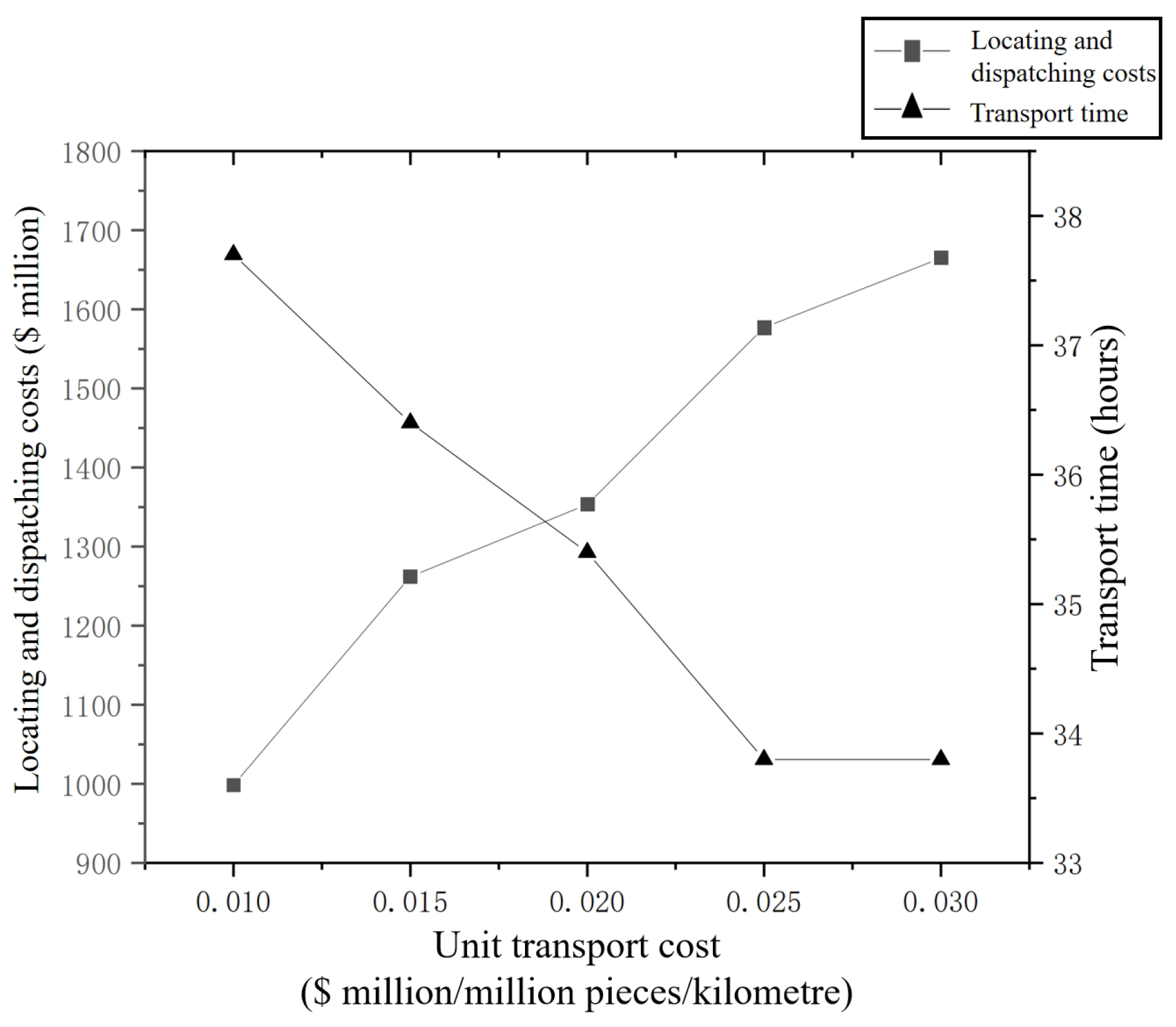
6.2.3. Sensitivity Analysis of Transportation Costs

In the previous research, this paper assumes that the transportation cost is a fixed value. However, in the actual rescue process, there may be road interruptions or insufficient transportation capacity, and these situations will dynamically affect the transportation cost. Therefore, in this section, a sensitivity analysis of transportation costs will be carried out to consider the impact of different transportation costs on the locating and dispatching cost, and transportation time of the MIP model. When solving for the location results, this section analyzes the change in the objective function in the range of transportation cost from USD 0.0014 million/per 10,000 units/km to USD 0.0042 million/per 10,000 units/km; the specific data are shown in

Table 9. Calculation results for different transport costs.

Cost Weighting	Transport Cost ${\mathit{c}}_{\mathit{t}}$	Locating and Dispatching	Emergency Transport
$\mathbf{\lambda }$	(USD Million/Million Units/km)	Cost  ${\mathbf{Z}}_{\mathbf{1}}$  (USD 10,000)	Time  ${\mathbf{Z}}_{\mathbf{2}}$  (h)
0.3	0.0014	139.79	37.7
0.3	0.0021	176.71	36.4
0.3	0.0028	189.45	35.4
0.3	0.0035	220.77	33.8
0.3	0.0042	233.07	33.8

and Figure 5.

It can be seen that, when the unit transportation cost $c_t$ is USD 0.0014–0.0035 million /10,000 units/km, as the unit transportation cost increases, the model locating and dispatching cost increases, while the transportation time decreases. It is worth noting that, when unit transportation cost $c_t$ takes USD 0.0021–0.0028 million/10,000 units/km, the slope of the change in locating and dispatching costs is smaller than other stages; this is due to the change in the location program caused by the increase in emergency logistics facilities but the corresponding transport distance is reduced, so the total cost of location and dispatching grows more slowly. When the unit transportation cost $c_t$ is more than USD 0.0035 million/10,000 units/km, the model of the locating and dispatching cost is still increasing, and the transportation time remains unchanged. This is because the increase in unit transportation cost only affects the locating and dispatching cost, which does not directly lead to the change in time due to the limitation of the weight coefficient.

From the above analysis, it can be seen that the model of locating and dispatching cost, transportation time, and unit transportation cost is linearly correlated with the change in unit transportation cost, which may lead to changes in the location program, which in turn affects the rate of change in the objective function. When the transportation time reaches a certain threshold, due to the limitation of the weight coefficient, the transportation time is not directly related to the unit transportation cost.

6.3. Analysis of Location Results in Uncertain Environments

6.3.1. Location Results for Stochastic Programming Models

First, set the location scenario and necessary parameters under an uncertain environment. In the stochastic programming model, it is assumed that emergency events have the following three demand scenarios: normal scale, large scale, and extreme scale. The demand change ranges corresponding to the three scenarios are $100\%$, $120\%$, and $150\%$ of the deterministic demand, respectively, with probabilities of $0.5$, $0.3$, and $0.2$. Similarly, it is assumed that the road congestion coefficient ${\sigma }_k$ set in this paper has three scenarios: normal, congested, and extremely congested. The corresponding values of ${\sigma }_k$ are 1, $1.5$, and 2, respectively, and the probabilities are the same as those of the demand scenarios, which are $0.5$, $0.3$, and $0.2$. Therefore, considering the randomness of both demand and road congestion coefficient simultaneously, nine emergency rescue scenarios K can be generated. The specific probability distribution corresponding to the nine scenarios in the stochastic programming model is shown in

Table 10. Probability distribution of random programming scenarios.

Road Conditions		Demand Scenarios
	${\mathit{D}}_{\mathbf{1}}$	${\mathit{D}}_{\mathbf{2}}$	${\mathit{D}}_{\mathbf{3}}$
${\sigma }_1$	$K_1$(0.25)	$K_2$(0.15)	$K_3$(0.1)
${\sigma }_2$	$K_4$(0.15)	$K_5$(0.09)	$K_6$(0.06)
${\sigma }_3$	$K_7$(0.1)	$K_8$(0.06)	$K_9$(0.04)

.

In the practical application of CVaR, a risk level that is too low cannot provide sufficient risk aversion and a risk level that is too high will bring a large amount of additional cost. In most literature, the range of risk level $\alpha$ is $[0.5,0.9]$. Therefore, in the RP-TSP proposed in this paper, the risk level $\alpha$ is set to $0.7$, and the values of ${\eta }_1$ and ${\eta }_2$ are, respectively, the transportation cost and transportation time under scenario $K_5$ (large-scale demand, road congestion). According to calculations, their values are USD 0.5117 million and 44.2 h, respectively. The method and environment for solving the model in this section are the same as in Section 6.3, so they will not be repeated. The location results of the two stochastic programming models are as follows:

(1) Location results of the TSP

The solution result of the TSP selected Chengdu, Deyang, Mianyang, Guangyuan, Meishan, and Ziyang, six places, where the total locating and dispatching cost $Z_1$ is USD 2.202 million, and the total transportation time $Z_2$ is 46.2 h. The specific emergency material allocation data are shown in

Table 11. Location results of the TSP model (ten thousand items).

Alternative Locations	Chengdu	Deyang	Mianyang	Guangyuan	Meishan	Ziyang
Wenchuan County	10
Beichuan County			12
Mianzhu		24
Qingchuan County				10
Mao County		12
Dujiangyan	29
Pingwu County				12
Pengzhou	18
Santai County			24
Lezhi County						12
Zhongjiang County		24
Renshou County						24
Zitong County			10
Yanting County			12
Hongya County					14
Ya’an City					24

. Through calculation, the facility utilization rates of each alternative point are, respectively, 71.3%, 100%, 96.7%, 36.7%, 76%, and 72%.

(2) Location results of RP-TSP

The solution result of the RP-TSP selected Chengdu, Deyang, Mianyang, Guangyuan, Meishan, and Ziyang, six emergency logistics facility alternative points, where the total locating and dispatching cost $Z_1$ is USD 2.244 million, and the total transportation time $Z_2$ is 51.5 h. The specific emergency material allocation data are shown in

Table 12. Location results of the TSP model based on risk preference (ten thousand items).

Alternative Locations	Chengdu	Deyang	Mianyang	Guangyuan	Meishan	Ziyang
Wenchuan County	10
Beichuan County			12
Mianzhu		24
Qingchuan County				10
Mao County			12
Dujiangyan	29
Pingwu County				12
Pengzhou	18
Santai County			24
Lezhi County						12
Zhongjiang County		24
Renshou County						24
Zitong County			10
Yanting County			12
Hongya County					14
Ya’an City					24

. Through calculation, the facility utilization rates of each alternative point are, respectively, 71.3%, 100%, 96.7%, 36.7%, 76%, and 72%.

It is not difficult to find that, compared with TSP, the demand for emergency materials and the number of locations in RP-TSP do not change, but the expected locating and dispatching cost, and transportation time increase due to considering the risk level which leads to an increase in the objective function. To further analyze the impact of risk level $\alpha$ on the objective function under the same expected transportation cost and transportation time, we will continue to study in depth through sensitivity analysis.

6.3.2. Location Results for Robust Optimization Models

In the robust optimization model, since there are 16 demand points considered in the case background, set $\Gamma =8$, the maximum disturbance range of demand is 50%, and the road congestion coefficient is 2. The method and environment for solving the model in this section are also the same as in Section 6.3 so they will not be repeated here.

The location results of two robust optimization models are as follows:

(1) Location results of RO-B

The solution result of the RO-B selected Chengdu, Deyang, Mianyang, Guangyuan, Meishan, Ziyang, and Suining as seven emergency logistics facility alternative points where total locating and dispatching cost $Z_1$ is USD 2.593 million and total transportation time $Z_2$ is 68.2 h. The specific emergency material allocation data are shown in

Table 13. Location results of the robust optimization model based on box uncertainty set (ten thousand items).

Alternative Locations	Chengdu	Deyang	Mianyang	Guangyuan	Meishan	Ziyang	Suining
Wenchuan County	12
Beichuan County			15
Mianzhu		30
Qingchuan County				12
Mao County			15
Dujiangyan	38
Pingwu County			15
Pengzhou	23
Santai County							30
Lezhi County						15
Zhongjiang County		30
Renshou County						30
Zitong County
Yanting County			12				15
Hongya County					18
Ya’an City					30

. Through calculation, the facility utilization rates of each alternative point are, respectively, $91.3\%,100\%,95\%,20\%,96\%,90\%,$ and $90\%$.

(2) Location results of RO-P

The location result of the RO-P selected Chengdu, Deyang, Mianyang Guangyuan Meishan, Ziyang, and Suining as seven emergency logistics facility alternative points where total locating and dispatching cost $Z_1$ is USD 2.498 million and total transportation time $Z_2$ is 68.2 h. The specific emergency material allocation data are shown in

Table 14. Location results of the robust optimization model based on polyhedral uncertainty set (ten thousand items).

Alternative Locations	Chengdu	Deyang	Mianyang	Guangyuan	Meishan	Ziyang	Suining
Wenchuan County	11
Beichuan County			13
Mianzhu		27
Qingchuan County				11
Mao County			13
Dujiangyan	35
Pingwu County			13
Pengzhou	20
Santai County							27
Lezhi County						13
Zhongjiang County		27
Renshou County						27
Zitong County			11
Yanting County							13
Hongya County					15
Ya’an City					27

. Through calculation, the facility utilization rates of each alternative point are, respectively, $82.5\%,90\%,83.3\%,18.3\%,84\%,80\%,$ and $80\%$.

It is not difficult to find that, in the results of the two types of uncertainty sets, the location results and transportation time are the same, but the locating and dispatching cost, and transportation volume have changed. This is due to the different robust conservatism which leads to changes in transportation costs. In terms of facility utilization rate, most emergency logistics facilities have reached more than 80; only Guangyuan has always maintained a lower level, which is caused by the distance between the Guangyuan facility alternative point and most demand points. In the following research, we will further explore the impact of robust conservatism $\Gamma$ on locating and dispatching cost, and transportation time through sensitivity analysis.

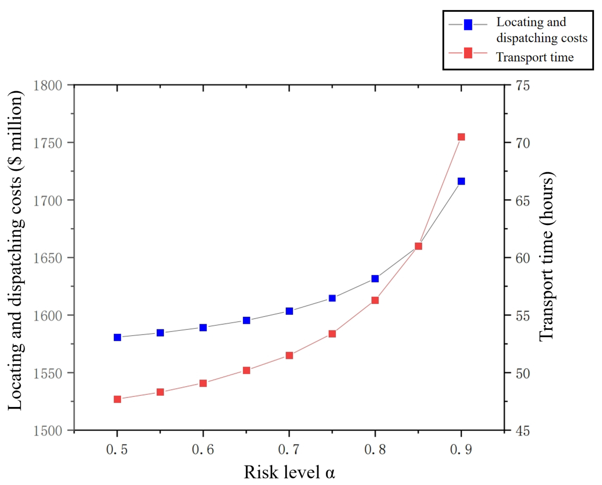
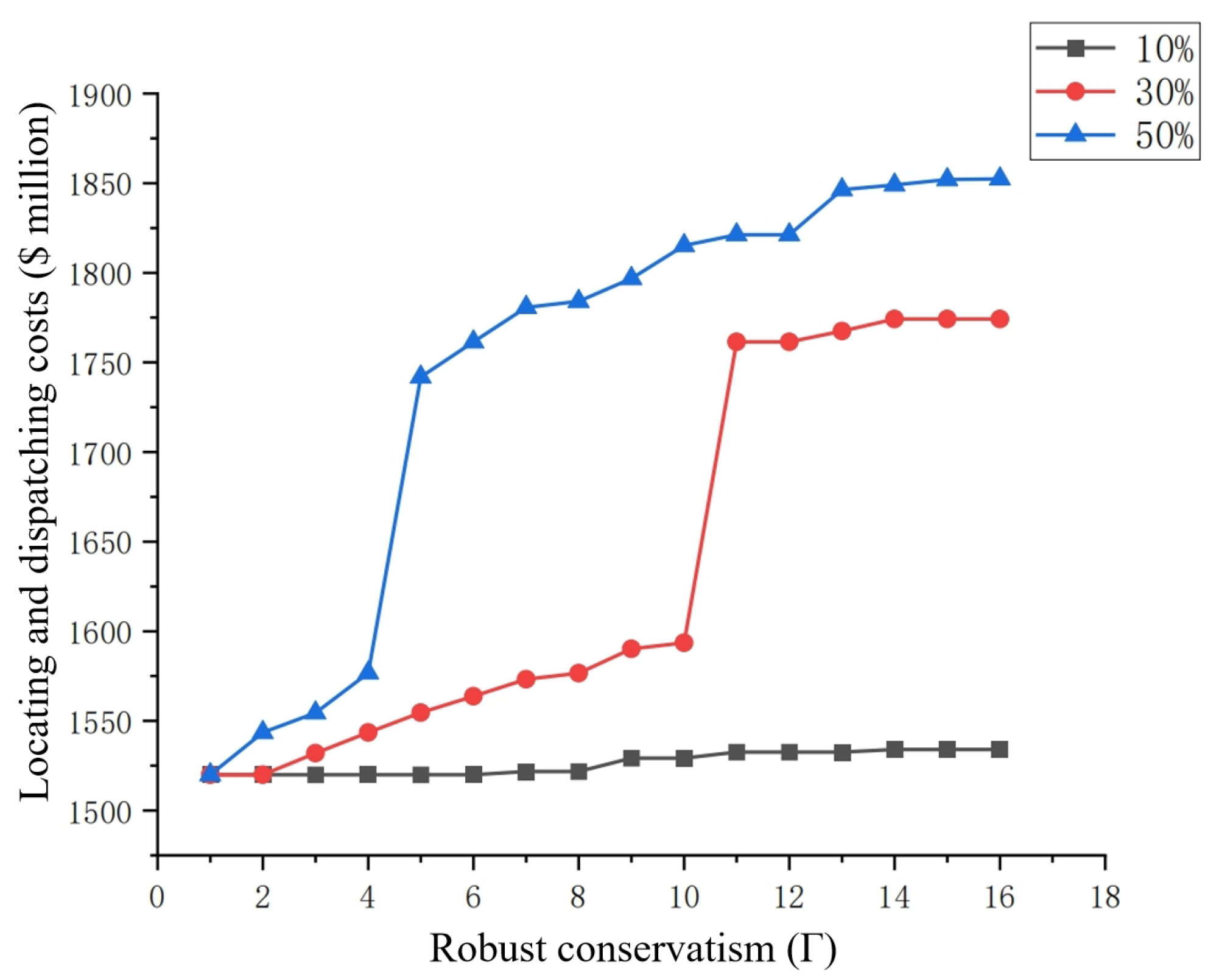
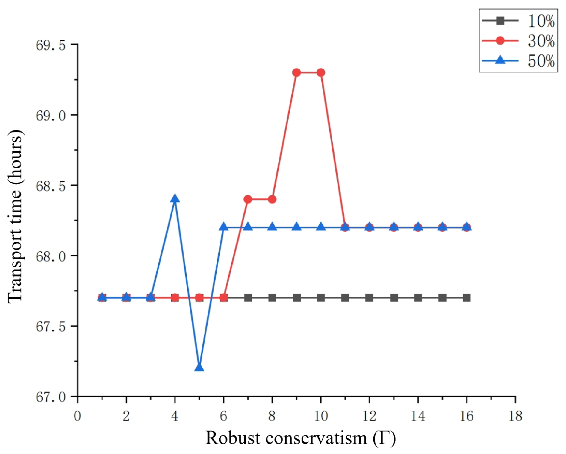
6.3.3. Sensitivity Analysis of Parameters in Uncertainty Models

This section will select two important parameters, risk level $\alpha$ and robust conservatism $\Gamma$, for sensitivity analysis of the established model.

(1) Impact of risk level $\alpha$ on the objective function

In previous studies, we assumed that the risk level is a fixed value. However, in the actual decision-making process, decision-makers need to make different degrees of additional cost input according to their risk preferences. Therefore, this section will conduct a sensitivity analysis of the risk level, considering the impact of different risk levels on the locating and dispatching cost, and transportation time in the RP-TSP model. In the previous discussion of this section, it was assumed that the risk level is 0.7. Therefore, this section will consider the change in locating and dispatching cost, and transportation time of emergency logistics facilities under different risk levels $\alpha$ in the interval $[0.5,0.9]$, and the specific results are shown in Figure 6.

As can be seen from Figure 6, as the risk level $\alpha$ increases, the corresponding locating and dispatching cost, and transportation time also increase, and, as $\alpha$ approaches 1, the rate of increase of the objective function also significantly increases. This also shows that at this time the decision-maker has a high aversion to risk and the RP-TSP model established has a high degree of risk aversion, which requires a large amount of cost and time. Therefore, decision-makers need to choose an appropriate risk level according to their risk preferences to avoid overly conservative solution results.

(2) Impact of robust conservatism $\Gamma$ on the objective function

To balance the robustness and economy of the emergency logistics facility location model, this section will analyze the changes in robust conservatism $\Gamma$ under different demand ranges for sensitivity analysis. Considering three different disturbance ranges, which are $10\%,30\%$, and $50\%$ of regular demand, respectively, demand will change within $110\%,130\%$, and $150\%$ of regular demand, respectively. The solution results are specifically shown in Figure 7 and Figure 8.

It can be seen that, as robust conservatism $\Gamma$ increases, the locating and dispatching cost of emergency logistics facilities continues to increase. Among them, the larger the disturbance range, the more significant the increase in locating and dispatching costs. This is because the greater the uncertainty, the more emergency supplies demand increases. It is worth mentioning that, in both cases where the disturbance range is 30% and 50%, there is a sudden large increase in locating and dispatching costs. This is because the original location scheme cannot meet changing demands and changes in location schemes.

In terms of transportation time, as robust conservatism $\Gamma$ increases, changes in transportation time are relatively small. This also shows that transportation time is not sensitive to changes in robust conservatism, proving that the model has strong time robustness. It should be noted that, when the disturbance range is 10%, there is no change in transportation time. However, when the disturbance range is 30% and 50%, there are some fluctuations in transportation time. The reason for this is similar to that of a large increase in locating and dispatching costs; both are due to changes in location schemes.

Looking at overall changes, in robust models, maximum locating and dispatching costs differ from minimum locating and dispatching costs by more than 20%. However, the shortest transportation times differ from the longest transportation times by no more than 3%. Therefore, when decision-makers use robust optimization methods for decision-making they need to prioritize factors such as locating and dispatching costs to determine corresponding robust conservatism.

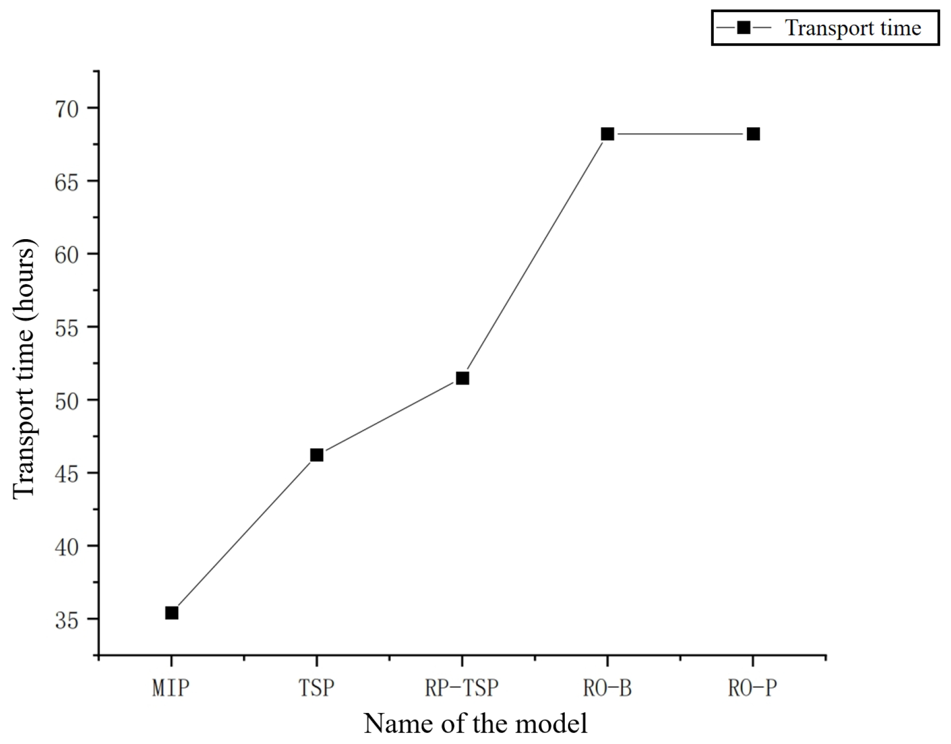
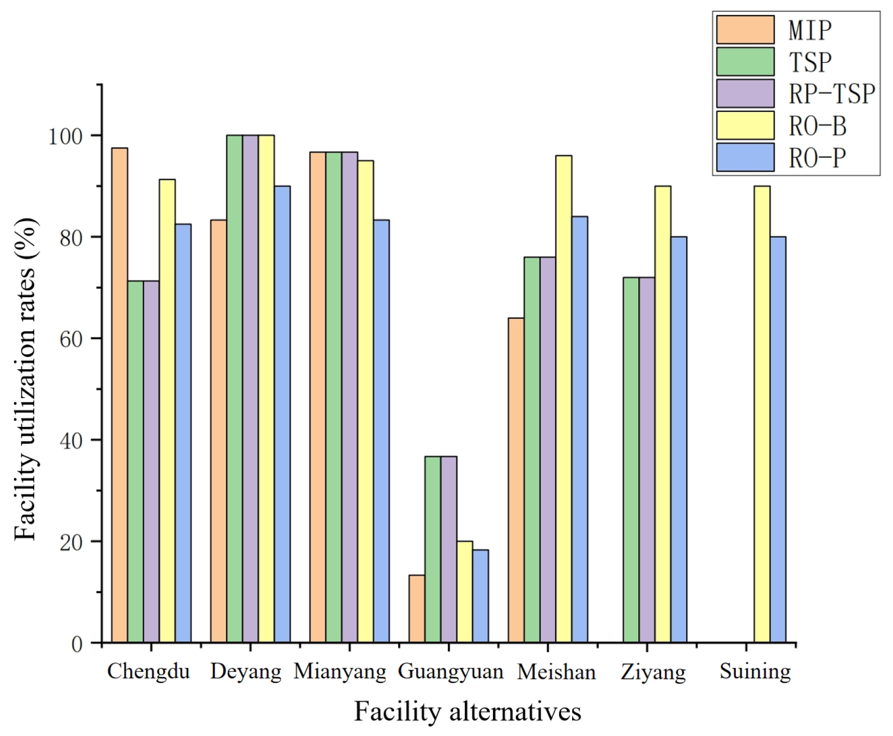
6.3.4. Comparative Analysis of Uncertainty Optimization Methods

To compare the rescue efficiency, economy, and stability of emergency logistics facility location models with different uncertainty optimization methods, this section will analyze four uncertainty models proposed in this section based on location results from Section 6.3 from three aspects: locating and dispatching cost, transportation time, and facility utilization rate. Through analysis, we can draw corresponding conclusions and provide corresponding management insights for decision-makers.

The four models are, respectively, TSP, RP-TSP, RO-B, and RO-P, proposed in Section 4 and Section 5. To further highlight characteristics of uncertainty models, we add results from the MIP of Section 3 for comparison considering two demand scenarios $(K_1,K_9)$ under MIP’s location results. It should be noted that, due to its conservatism, RO-B’s location result is the same as MIP under scenario $K_9$. Therefore, during the analysis process, we no longer list MIP’s result under $K_9$ separately.

First is the locating and dispatching cost. As can be seen from Figure 9, models considering uncertain environments all produce higher locating and dispatching costs than deterministic models. Stochastic programming models produce less additional locating and dispatching costs than robust models. Among them, RP-TSP has a slight increase in locating and dispatching cost compared to TSP, which is due to consideration of tail-end extreme risks leading to cost increase. In robust models, RO-B is the most conservative. Since RO-P can adjust robust conservatism, it is relatively more economical in terms of economy, but the locating and dispatching cost of RO-P is still much higher than that of the stochastic programming model.

In terms of transportation time, as can be seen from Figure 10, models considering uncertain environments still produce higher transportation time than deterministic models. This is because MIP does not consider the possibility of road congestion. Stochastic programming models produce less transportation time than robust models. However, RP-TSP differs more in transportation time from TSP than in locating and dispatching costs. This shows that RP-TSP has a greater sensitivity to changes in transportation time. RO-B and RO-P have the same results in terms of transportation time. This shows that robust conservatism in the model set in this paper does not have a large impact on transportation time and also proves the stability of this transportation time solution result.

In terms of facility utilization rate, Figure 11 shows facility utilization rates of seven facility alternative points in different models. Among them, MIP selected five facility points, the TSP and RP-TSP models both selected six facility points, and RO-B and RO-P both selected seven facility points. All location models have higher facility utilization rates in Chengdu, Deyang, Mianyang, and Meishan, all exceeding 60%. However, location schemes for Guangyuan, Ziyang, and Suining are different. Among them, Guangyuan’s facility utilization rate is generally low. This is because this facility point has a large distance from most demand points and exceeds the maximum service distance $d_{\max }$ set by the model. MIP did not select Ziyang, and only RO-B and RO-P selected Suining.

Through analysis and comparison, it can be known that the number of locations under uncertain environment models is more than that under deterministic environment models. In uncertain environment models, the stochastic programming model has fewer locations and its average facility utilization rate is between two robust models. Because of its conservatism, the RO-B model considers worst-case demand changes so its facility utilization rate is higher. The RO-P model controls conservatism relative to the RO-B model but because the final location scheme is the same it leads to a larger surplus for each emergency logistics facility.

In summary, by analyzing four uncertainty optimization models proposed in this paper from three aspects, locating and dispatching cost, transportation time, and facility utilization rate, this section draws the following conclusions: Firstly, to cope with widespread uncertainty in emergency logistics application scenarios, decision-makers need to pay a certain price such as higher locating and dispatching costs, and more expected transportation time. However, when extreme disaster scenarios occur models considering uncertainty have more advantages in expected locating and dispatching costs. and transportation time. Secondly, among the two uncertainty optimization methods, stochastic programming has better economy and less expected transportation time, and its facility utilization rate is between the two robust models. The RP-TSP model has a certain degree of risk aversion so both its locating and dispatching cost, and transportation time are increased compared to TSP. Robust optimization has better robustness among which RO-P has a certain reduction in locating and dispatching cost compared to RO-B which can effectively avoid the over-conservatism of RO-B.

6.4. Management Insights

Through analysis and summary of conclusions from Section 6.3 and Section 6.4, this section also gives corresponding management insights for decision-makers as follows:

(1) Reasonably allocate locating and dispatching costs, and transportation time weights

When decision-makers face emergency logistics facility location problems, they need to consider many factors. Firstly, the service target of emergency logistics is different from traditional logistics so rescue efficiency should be given more attention compared to economic cost. Therefore, the people-oriented target is very important so transportation time needs to have more weight than locating and dispatching costs in most cases. In addition, the weight coefficient needs to be adjusted within a reasonable value range; too high or too low a $\lambda$ may not cause changes in the objective function leading to invalid cost expenditure.

(2) Scientifically set expected cost and risk level

When choosing locations for emergency logistics facilities, it is important to fully consider potential extreme situations. Although the probability of extreme risks occurring is relatively small, once they occur, the losses caused will be far higher than the average level. This requires decision-makers to weigh between cost and risk. On the other hand, the location of emergency logistics facilities belongs to public welfare facilities and cannot make a profit. Excessive robustness often leads to a significant increase in costs, bringing considerable economic pressure to relevant governments and enterprises. Therefore, when using RP-TSP for location, it is necessary to choose an appropriate expected cost and risk level based on historical data, the decision-makers’ risk preferences, etc., thereby avoiding losses caused by extreme risks and excessive cost input at the same time.

(3) Decision-makers should choose uncertainty optimization methods according to their risk preferences

In the location of emergency logistics facilities, uncertainty is widespread. When faced with uncertainty, decision-makers should choose optimization methods that suit their personal risk preferences. This means that, in the decision-making process, decision-makers need to consider their tolerance for risk and their expectations for the results. Some decision-makers are willing to take certain risks, and hope to reduce the cost of location and dispatching through high-risk, low-input schemes, which are more suitable for using stochastic programming methods. On the other hand, some risk-averse decision-makers prefer stable and reliable results, which are more suitable for using robust optimization methods. The RP-TSP model proposed in this paper combines the advantages of the high economic efficiency of stochastic programming and the high stability of robust optimization, providing a new method for decision-makers to select emergency logistics facilities in uncertain environments.

Emergency logistics, management methods, and technical methods should be coordinated in a harmonious and efficient manner to ensure the successful operation of the emergency logistics system. Emergency logistics involves the strategic placement of emergency facilities, efficient routing of emergency vehicles, and timely delivery of emergency supplies. It requires careful planning and execution, taking into account various factors such as geographical constraints, traffic conditions, and the urgency of the situation. Management methods include strategies and policies for managing the logistics system, such as risk management, resource allocation, and decision-making processes. Effective management ensures that the logistics operations are carried out smoothly and efficiently, with minimal delays and errors. Technical methods involve the use of technology and mathematical models to optimize the logistics operations. For example, mixed-integer programming can be used to determine the optimal locations for emergency facilities and simulation techniques can be used to predict the outcomes of different logistics strategies.

To coordinate these elements effectively, communication is key. All parties involved in the logistics operations should communicate regularly and share information freely. This ensures that everyone is on the same page and working towards the same goals. Integration of logistics, management, and technical aspects is crucial. This means that the logistics operations should be guided by the management strategies and supported by the technical methods. For example, the placement of emergency facilities (a logistics decision) should be based on risk management strategies (a management decision) and determined using mixed-integer programming (a technical method). Adaptability is also important. The logistics system should be flexible enough to adapt to changing circumstances, such as a sudden increase in demand for emergency supplies. This requires both robust management strategies and versatile technical methods.

In conclusion, the coordination of emergency logistics, management methods, and technical methods is a complex task that requires careful planning, effective communication, and the judicious use of technology. But, when done right, it can greatly enhance the efficiency of the emergency logistics system and ensure the timely delivery of emergency supplies.

7. Conclusions

In conclusion, this study addresses the critical issue of emergency logistics facilities located in the face of uncertainties arising from natural disasters and public health events. We developed single-objective and dual-objective MIPs for location, considering factors such as construction cost, emergency rescue human resource dispatching cost, storage cost, and transportation cost. We further incorporated stochastic programming, risk functions, and robust optimization to handle uncertainties in demand and road conditions. Our models were validated using the Gurobi solver, providing new research methods for decision-makers and offering more scientific theoretical guidance.

Our study revealed that the weight values in the dual-objective model and the unit transportation cost significantly impact the objective function. Decision-makers should select appropriate weighting factors to balance the effectiveness and affordability of emergency response at different stages, which will enhance the overall sustainability of the emergency logistics system. Our sensitivity analysis showed that the risk function can effectively measure the impact of tail extreme risks at different risk levels on the objective function, which is beneficial for decision-makers with different risk preferences.

However, our research has certain limitations. First, although we considered many factors in the modeling process of emergency logistics facility locating, all cost functions considered in this paper are linear functions, which are dynamic in actual situations. Second, we assumed that the type of emergency supplies is unique but, in actual rescue processes, there may be more types involved, such as first aid kits, tents, etc., and different regions have different demands for different types of supplies. Third, we assumed that the established emergency logistics model is reliable but, in actual application scenarios of emergency logistics, there may be possibilities of network interruption.

Therefore, future research can consider these situations comprehensively and explore the problem of emergency logistics facility locating more deeply. Despite these limitations, our study provides a new approach for decision-makers to solve the problem of emergency logistics facilities sitting under uncertain environments by combining the high economic efficiency of stochastic programming and the high stability of robust optimization.

References

1. Yaghmaei, N. Human Cost of Disasters: An Overview of the Last 20 Years, 2000–2019; UN Office for Disaster Risk Reduction: Geneva, Switzerland, 2020. [Google Scholar]
2. OCHA. Global Humanitarian Overview 2022. 2021. Available online: https://2022.gho.unocha.org/ (accessed on 1 November 2021).
3. Kovacs, G.; Moshtari, M. A roadmap for higher research quality in humanitarian operations: A methodological perspective. Eur. J. Oper. Res. 2019, 276, 395–408. [Google Scholar] [CrossRef]
4. Trunick, P. Special report: Delivering relief to tsunami victims. Logist. Today 2005, 46, 1–3. [Google Scholar]
5. Van Wassenhove, L. Humanitarian aid logistics: Supply chain management in high gear. J. Oper. Res. Soc. 2006, 57, 475–489. [Google Scholar] [CrossRef]
6. Sahebjamnia, N.; Torabi, S.; Mansouri, S. A hybrid decision support system for managing humanitarian relief chains. Decis. Support Syst. 2017, 95, 12–26. [Google Scholar] [CrossRef]
7. Kundu, T.; Sheu, B.; Kuo, H. Emergency logistics management—Review and propositions for future research. Transp. Res. Part E Logist. Transp. Rev. 2022, 164, 102789. [Google Scholar] [CrossRef]
8. Kovács, G.; Spens, K. Humanitarian logistics in disaster relief operations. Int. J. Phys. Distrib. Logist. Manag. 2006, 37, 99–114. [Google Scholar] [CrossRef]
9. Knott, R. Humanitarian aid logistics: Supply chain management in high gear. Disasters 1987, 11, 113–115. [Google Scholar] [CrossRef]
10. Barbarosoglu, G.; Arda, Y. A two-stage stochastic programming framework for transportation programming in disaster response. J. Oper. Res. Soc. 2004, 55, 43–53. [Google Scholar] [CrossRef]
11. Beamon, B.; Kotleba, S. Inventory modeling for complex emergencies in humanitarian relief operations. Int. J. Logist. Res. Appl. 2006, 9, 1–18. [Google Scholar] [CrossRef]
12. Paul, J.; MacDonald, L. Optimal location, capacity and timing of stockpiles for improved hurricane preparedness. Int. J. Prod. Econ. 2016, 174, 11–28. [Google Scholar] [CrossRef]
13. Paul, J.; Wang, X. Robust location-allocation network design for earthquake preparedness. Transp. Res. Part B Methodol. 2019, 119, 139–155. [Google Scholar] [CrossRef]
14. Shen, L.; Tao, F.; Shi, Y. Optimization of location-routing problem in emergency logistics considering carbon emissions. Int. J. Environ. Res. Public Health 2019, 16, 2982. [Google Scholar] [CrossRef]
15. Du, J.; Wu, P.; Wang, Y.; Yang, D. Multi-stage humanitarian emergency logistics: Robust decisions in uncertain environment. Nat. Hazards 2023, 115, 899–922. [Google Scholar] [CrossRef]
16. Altay, N.; Kovács, G.; Spens, K. The evolution of humanitarian logistics as a discipline through a crystal ball. J. Humanit. Logist. Supply Chain Manag. 2021, 11, 577–584. [Google Scholar] [CrossRef]
17. Kovacs, G.; Spens, K.M. (Eds.) Relief Supply Chain Management for Disasters: Humanitarian Aid and Emergency Logistics; Information Science Reference: Hershey, PA, USA, 2011. [Google Scholar]
18. Basharat, M.; Riaz, M.; Jan, M.; Xu, C.; Riaz, S. A review of landslides related to the 2005 Kashmir Earthquake: Implication and future challenges. Nat. Hazards 2021, 108, 1–30. [Google Scholar] [CrossRef]
19. Huang, K.; Jiang, Y.; Yuan, Y.; Zhao, L. Modeling multiple humanitarian objectives in emergency response to large-scale disasters. Transp. Res. Part E Logist. Transp. Rev. 2015, 75, 1–17. [Google Scholar] [CrossRef]
20. Liu, Y.; Cui, N.; Zhang, J. Integrated temporary facility location and casualty allocation planning for post-disaster humanitarian medical service. Transp. Res. Part E Logist. Transp. Rev. 2019, 128, 1–16. [Google Scholar] [CrossRef]
21. Sun, H.; Li, Y.; Zhang, J. Collaboration-based reliable optimal casualty evacuation network design for large-scale emergency preparedness. Socio-Econ. Program. Sci. 2022, 81, 101192. [Google Scholar] [CrossRef]
22. Ghasemi, P.; Khalili-Damghani, K.; Hafezalkotob, A.; Raissi, S. Stochastic optimization model for distribution and evacuation programming (A case study of Tehran earthquake). Socio-Econ. Program. Sci. 2022, 71, 100745. [Google Scholar]
23. Paul, J.; Zhang, M. Supply location and transportation programming for hurricanes: A two-stage stochastic programming framework. Eur. J. Oper. Res. 2019, 274, 108–125. [Google Scholar] [CrossRef]
24. Wang, L. A two-stage stochastic programming framework for evacuation programming in disaster responses. Comput. Ind. Eng. 2020, 145, 106458. [Google Scholar] [CrossRef]
25. Oksuz, M.; Satoglu, S. A two-stage stochastic model for location planning of temporary medical centers for disaster response. Int. J. Disaster Risk Reduct. 2020, 44, 101426. [Google Scholar] [CrossRef]
26. Aydin, N. A stochastic mathematical model to locate field hospitals under disruption uncertainty for large-scale disaster preparedness. Int. J. Optim. Control 2016, 6, 85–102. [Google Scholar] [CrossRef]
27. Manopiniwes, W.; Irohara, T. Stochastic optimisation model for integrated decisions on relief supply chains: Preparedness for disaster response. Int. J. Prod. Res. 2017, 55, 979–996. [Google Scholar] [CrossRef]
28. Ben-tal, A.; Nemirovski, A. Robust Convex Optimization. Math. Oper. Res. 1998, 23, 769–805. [Google Scholar] [CrossRef]
29. Li, Y.; Zhang, J.; Yu, G. A scenario-based hybrid robust and stochastic approach for joint programming of relief logistics and casualty distribution considering secondary disasters. Transp. Res. Part E Logist. Transp. Rev. 2020, 141, 102029. [Google Scholar] [CrossRef]
30. Najafi, M.; Eshghi, K.; Dullaert, W. A multi-objective robust optimization model for logistics planning in the earthquake response phase. Transp. Res. Part E Logist. Transp. Rev. 2013, 49, 217–249. [Google Scholar] [CrossRef]
31. Ni, W.; Shu, J.; Song, M. Location and emergency inventory pre-positioning for disaster response operations: Min-max robust model and a case study of Yushu earthquake. Prod. Oper. Manag. 2018, 27, 160–183. [Google Scholar] [CrossRef]
32. Balcik, B.; Yanikoglu, I. A robust optimization approach for humanitarian needs assessment planning under travel time uncertainty. Eur. J. Oper. Res. 2020, 282, 40–57. [Google Scholar] [CrossRef]
33. Ke, G. Managing reliable emergency logistics for hazardous materials: A two-stage robust optimization approach. Comput. Oper. Res. 2022, 138, 105557. [Google Scholar] [CrossRef]
34. Basak, S.; Shapiro, A. Value-at-risk-based risk management: Optimal policies and asset prices. Rev. Financ. Stud. 2001, 14, 371–405. [Google Scholar] [CrossRef]
35. Jin, T.; Yang, X. Monotonicity theorem for the uncertain fractional differential equation and application to uncertain financial market. Math. Comput. Simul. 2021, 190, 203–221. [Google Scholar] [CrossRef]
36. Rockafellar, R.; Wets, R. Stochastic variational inequalities: Single-stage to multistage. Math. Program. 2017, 165, 331–360. [Google Scholar] [CrossRef]
37. Jin, T.; Xia, H. Lookback option pricing models based on the uncertain fractional-order differential equation with Caputo type. J. Ambient Intell. Humaniz. Comput. 2023, 14, 6435–6448. [Google Scholar] [CrossRef]
38. Qu, S.; Li, S. A supply chain finance game model with order-to-factoring under blockchain. Syst. Eng. Theory Pract. 2023, 41, 1–16. [Google Scholar]
39. Ji, Y.; Ma, Y. The robust maximum expert consensus model with risk aversion. Math. Program. 2023, 99, 101866. [Google Scholar] [CrossRef]
40. Ahmed, S. Convexity and decomposition of mean-risk stochastic programs. Math. Program. 2006, 106, 433–446. [Google Scholar] [CrossRef]
41. Miller, N.; Ruszczyński, A. Risk-averse two-stage stochastic linear programming: Modeling and decomposition. Oper. Res. 2011, 59, 125–132. [Google Scholar] [CrossRef]
42. Xu, X.; Yan, Z.; Shahidehpour, M.; Li, Z.; Yan, M.; Kong, X. Data-Driven Risk-Averse Two-Stage Optimal Stochastic Scheduling of Energy and Reserve With Correlated Wind Power. IEEE Trans. Sustain. Energy 2020, 11, 436–447. [Google Scholar] [CrossRef]
43. Das, D.; Verma, P.; Tanksale, A. Designing a closed-loop supply chain for reusable packaging materials: A risk-averse two-stage stochastic programming model using CVaR. Comput. Ind. Eng. 2022, 167, 108004. [Google Scholar] [CrossRef]
44. Lewis, C. Linear Programming: Theory and Applications. 2008, pp. 1–66. Available online: https://www.whitman.edu/documents/Academics/Mathematics/lewis.pdf (accessed on 11 May 2008).
45. Meyer, R. On the existence of optimal solutions to integer and mixed-integer programming problems. Math. Program. 1974, 7, 223–235. [Google Scholar] [CrossRef]
46. Martínez-Legaz, J. On Weierstrass extreme value theorem. Optimization Letters. J. Risk 2014, 8, 391–393. [Google Scholar]
47. Huang, M.; Huang, L.; Zhong, Y.; Yang, H.; Chen, X.; Huo, W.; Shi, L. MILP Acceleration: A Survey from Perspectives of Simplex Initialization and Learning-Based Branch and Bound. J. Oper. Res. Soc. China 2023, 1, 1–42. [Google Scholar] [CrossRef]
48. Rockafellar, R.; Uryasev, S. Optimization of conditional value-at-risk. J. Risk 2000, 2, 21–42. [Google Scholar] [CrossRef]
49. Soyster, A.L. Convex programming with set-inclusive constraints, and application to inexact LP. Oper. Res. 1973, 21, 1154–1157. [Google Scholar] [CrossRef]
50. Feng, J.; Gai, W.; Li, J.; Xu, M. Location selection of emergency supplies repositories for emergency logistics management: A variable weighted algorithm. J. Loss Prev. Process Ind. 2020, 63, 104032. [Google Scholar] [CrossRef]
51. Ding, Z.; Xu, X.; Jiang, S.; Yan, J.; Han, Y. Emergency logistics scheduling with multiple supply-demand points based on grey interval. J. Saf. Sci. Resil. 2022, 3, 179–188. [Google Scholar] [CrossRef]
52. Wang, Y.; Wang, X.; Fan, J.; Wang, Z.; Zhen, L. Emergency logistics network optimization with time window assignment. Expert Syst. Appl. 2023, 214, 119145. [Google Scholar] [CrossRef] [PubMed]
53. Jiang, Y.; Yuan, Y. International Journal of Environmental Research and Public Health. Expert Syst. Appl. 2019, 16, 779. [Google Scholar]
54. Jiang, Y.; Yuan, Y.; Huang, K.; Zhao, L. Logistics for Large-Scale Disaster Response: Achievements and Challenges. In Proceedings of the 2012 45th Hawaii International Conference on System Sciences, Maui, HI, USA, 4–7 January 2012; pp. 1277–1285. [Google Scholar]
55. Wang, F.; Ge, X.; Li, Y.; Zheng, J.; Zheng, W. Optimising the Distribution of Multi-Cycle Emergency Supplies after a Disaster. Sustainability 2023, 15, 902. [Google Scholar] [CrossRef]
56. Ghasemi, P.; Goodarzian, F.; Abraham, A. A new humanitarian relief logistic network for multi-objective optimization under stochastic programming. Appl. Intell. 2022, 52, 13729–13762. [Google Scholar] [CrossRef] [PubMed]
57. Zheng, W.; Zhou, H. Robust dual sourcing inventory routing optimization for disaster relief. PLoS ONE 2023, 18, e0284971. [Google Scholar] [CrossRef] [PubMed]
58. Sarma, D.; Bera, U.; Singh, A.; Maiti, M. A multi-objective post-disaster relief logistic model. In Proceedings of the 2017 IEEE Region 10 Humanitarian Technology Conference (R10-HTC), Dhaka, Bangladesh, 21–23 December 2017; pp. 205–208. [Google Scholar]
Figure 1. Schematic diagram of emergency logistics facility location problem.
Sustainability 16 01361 g001
Figure 2. Schematic diagram of the geographical location of the case background.
Sustainability 16 01361 g002
Figure 3. Abstract model map of the case background.
Sustainability 16 01361 g003
Figure 4. Calculation results under different weights.
Sustainability 16 01361 g004
Figure 5. Calculation results for different transportation costs.
Sustainability 16 01361 g005
Figure 6. Effect of risk level on the objective function.
Sustainability 16 01361 g006
Figure 7. Impact of robust conservatism on locating and dispatching costs.
Sustainability 16 01361 g007
Figure 8. Impact of robust conservatism on transportation time.
Sustainability 16 01361 g008
Figure 9. Comparison of locating and dispatching costs under different models.
Sustainability 16 01361 g009
Figure 10. Comparison of transportation time under different models.
Sustainability 16 01361 g010
Figure 11. Facility utilization under different models.
Sustainability 16 01361 g011