Abstract
With environmental degradation and energy shortages, green and low-carbon development has become an industry trend, especially in regards to cold chain logistics (CCL), where energy consumption and emissions are substantial. In this context, determining how to scientifically evaluate the cold chain logistics efficiency (CCLE) under carbon emission constraints is of great significance for achieving sustainable development. This study uses the three-stage data envelopment analysis (DEA) and the Malmquist index model to analyze the overall level and regional differences regarding CCLE in China’s four major urban agglomerations, under carbon constraints, from 2010 to 2020. Then, the influencing factors of CCLE are identified through Tobit regression. The results reveal that: (1) the CCLE in the four urban agglomerations is overestimated when carbon constraints are not considered; (2) the CCLE in the four urban agglomerations shows an upward trend from 2010 to 2020, with an average annual growth rate of 1.25% in regards to total factor productivity. However, there are significant spatial and temporal variations, with low-scale efficiency being the primary constraint. (3) Different influencing factors have different directions and exert different effects on CCLE in different urban agglomerations, and the improvement of economic development levels positively affects all regions.
1. Introduction
The issue of global warming caused by greenhouse gas emissions, especially carbon dioxide, is one of the most significant challenges currently facing humanity. Countries around the world are focusing extensive attention on this problem [1,2]. China has consecutively become the world’s largest energy consumer and greenhouse gas emitter, with its energy-related carbon dioxide emissions reaching about 12.1 billion tonnes in 2022, accounting for 32.88% of the global share [3]. Faced with significant pressure to reduce emissions, China’s government has committed to peak carbon emissions by 2030 and achieve carbon neutrality by 2060 [4], and is currently implementing a range of measures to reduce emissions across all industries, including cold chain logistics (CCL).
CCL, as a branch of the logistics industry exhibiting high energy consumption and carbon emissions, plays a crucial role in reducing carbon emissions [5]. In contrast to traditional logistics, CCL requires significant amounts of petrochemical or electrical energy to maintain a constant and stable low-temperature environment, which is necessary to ensure the quality and safety of the products being transported. According to statistics, China’s post-harvest cold chain for fresh produce consumes CNY 80 billion worth of electrical energy annually for low-temperature refrigeration. Furthermore, emissions from transport vehicles, such as refrigerated trucks and containers, as well as refrigerant leakage, contribute to the problem of cold chain emissions [6]. However, the potential market for the development of CCL in China is expanding rapidly due to the acceleration of urbanization and the diversification of the consumption structure. In 2021, the market scale was CNY 418 billion, indicating a stable growth trend with a year-on-year increase of 9.2%, which presents valuable opportunities for the development of China’s CCL, but also poses significant challenges. The reduction of energy consumption and carbon emissions, while maintaining the efficiency of operations, is a crucial issue that needs to be addressed as a matter of urgency in the development of CCL.
Although the future of CCL in China is promising, there are still issues that hinder its development, such as low efficiency, poor quality, and regional imbalance [7]. The “14th Five-Year Plan” for the development of cold chain logistics, issued by the State Council, emphasizes the importance of accelerating operational efficiency improvement and reducing emissions to achieve high-quality development [8]. Some scholars have noted that logistics efficiency is a significant indicator for evaluating the quality of logistics development, and measuring logistics efficiency is the initial step to elevating the level of logistics development [9]. However, the literature review reveals that existing studies mostly concentrate on efficiency measurement related to conventional logistics, with fewer studies focused on CCL. Therefore, determining a method to scientifically and accurately measure the cold chain logistics efficiency (CCLE) from a low-carbon perspective, identify the key factors affecting efficiency improvement, and formulate targeted improvement strategies accordingly has become an important target to promote the efficient, balanced, and low-carbon development of regional CCL and to help China achieve its dual-carbon goal.
In these contexts, based on the three-stage DEA model, the Malmquist index model, and the Tobit regression model, we constructed a regional CCLE measurement model and influence factor analysis model under the carbon constraint and carried out an empirical analysis of major urban clusters in China. Then, we comprehensively conducted a static and dynamic combination of spatiotemporal evolution law exploration and difference analysis, suggesting targeted recommendations based on the results of the analysis of the influencing factors, which are helpful for the green, low-carbon, efficient, and balanced development of CCL.
The remainder of the paper is organized as follows. Section 2 is a review of the related literature. Section 3 introduces the basic theory and methods of this paper. The construction of the evaluation indicators and the collected data are described in Section 4. Section 5 presents the empirical study and analysis of the results, including static, dynamic, and driving factors analysis. Section 6 provides the conclusions and management insights.
2. Literature Review
Logistics efficiency is an important indicator of logistics resources input and effective output, which can reflect the overall development of the industry. The literature review includes two aspects: the CCLE measurement and promotion strategy.
2.1. Measurement of CCLE
According to existing studies, researchers have employed stochastic frontier analysis (SFA), data envelopment analysis (DEA), analytic hierarchical analysis (AHP), and other methods to measure logistics efficiency. The research subjects are mainly traditional logistics systems, with less research in regards to CCL. Park and Lee [10] measured the logistics efficiency of 14 Korean logistics suppliers. Based on the corporate perspective, other scholars used AHP and DEA to estimate the efficiency of reverse logistics operations for construction companies and third-party logistics companies, respectively [11,12]. In addition, Liang [13] considered the carbon emissions of the logistics industry and measured the logistics efficiency of 13 cities in Jiangsu Province from a city perspective. Barilla [14] measured total factor logistics productivity in Italy from a national perspective.
Among many methods, the DEA model is widely used in the logistics field because it does not require the construction of a specific form of the model and can solve the problem of multiple inputs and outputs. However, with the expansion and deepening of the research scope, the limitations of the DEA model have gradually emerged, and the method cannot remove the defects of the external environment and the random error terms.
In response to these defects, many scholars have proposed different optimization strategies, such as the BCC-DEA model [15,16], the Super-SBM model [17,18], and the DEA environmental assessment model [19]. The main input indicators include the capital stock in the logistics industry [13,20], the number of employees in the logistics industry [21], infrastructure development (road mileage, railway mileage, etc.) [14,22], and key output indicators such as freight volume and cargo turnover [23]. With the increasingly prominent environmental problems, many scholars have incorporated environmental indicators, such as energy consumption and carbon emissions, into the efficiency evaluation index system to adapt to the trend of sustainable development [24,25]. However, research on the measurement of CCLE under energy and environmental constraints remains to be supplemented.
2.2. Promotion Strategy of CCLE
At present, the research on CCLE enhancement is mainly focused on optimizing the CCL network, or proposing optimization strategies from a single aspect such as transportation, distribution, or warehousing. In terms of network optimization, Wu and Zhu [26] constructed a CCL network optimization model based on the hub and spoke theory to improve efficiency. Yu [27] constructed an international CCL network to reduce costs and increase efficiency. In terms of single link optimization, Li [28] suggested that with the promotion of intelligent logistics and joint distribution, the introduction of advanced technologies can effectively improve the distribution efficiency in CCL. Some researchers have also considered the integrity of the CCL, proposing a two-stage optimization model to improve CCLE and enhance customer satisfaction [29,30,31]. In general, there are few studies regarding improving the overall CCLE of the region, and the existing literature mostly focuses on qualitative analysis, lacking quantitative research.
2.3. Literature Review and Summary
Through a review and summary of the relevant research, we find that most of the existing studies on logistics efficiency focus on the traditional logistics industry, with little attention paid to the rapidly developing CCL in recent years. On the other hand, the research on CCLE improvement takes a single perspective, focusing on network construction optimization or single link optimization, and the quantitative and comprehensive measurement and analysis of CCLE from a holistic level still requires expansion. Furthermore, the evaluation index system for CCLE measurement is constructed in such a way that the impact of environmental and energy constraints on CCLE is ignored. Empirical research indicates that there is a lack of research and differential analysis in regards to urban agglomerations.
Therefore, this study examines CCL from a low-carbon perspective using a three-stage DEA model, a Malmquist index model, and a Tobit regression model to construct an efficiency measurement and influencing factor analysis framework. In contrast to previous research, the contributions of this paper are as follows: (1) empirical analyses on the CCLE at the urban cluster level are conducted; (2) in constructing the evaluation index system, the specific characteristics and development trends of CCL are taken into account, with carbon emissions as an input variable in the analysis framework. This not only enriches and supplements the existing body of knowledge on CCL evaluation theory, but also serves as a valuable reference for the advancement of the CCL industry in other regions.
3. Methodology
Based on data obtaining, this paper combined the three-stage DEA and Malmquist index model to measure CCLE and applied the Tobit regression model to analyze influencing factors. The basic theories and methods used are as follows.
3.1. Three-Stage DEA Model
To compensate for the fact that traditional DEA model does not take into account the effects of environmental factors and random errors, Fried [32] constructed a three-stage DEA model by incorporating environmental variables, random errors, and management inefficiency terms into the efficiency analysis framework. Therefore, we used the three-stage DEA model to measure the CCLE, and the specific steps are as follows.
(1) The first stage is using the traditional DEA model to analyze the initial efficiency. We selected the input-oriented BCC model. For any decision-making unit, the BCC model, in dual form, can be expressed as follows:
where, represents the decision-making units, and are the input and output vectors, , represent the input and output relaxation variables, represents the non-Archimedean infinitesimal, is the decision variable, and denotes the comprehensive efficiency value of the decision-making units.
(2) The second stage is to use SFA-like regression to remove environmental factors and noise. In this stage, the effects of environmental factors and random disturbances are removed by constructing the following model to make the measurement results more accurate (Equation (2)).
where is the relaxation value of the input of the decision-making unit, represents the environmental variable, represents the environmental variable coefficient, represents the mixed error term, and the former represents random interference, while the latter represents management inefficiency (, ).
In the separation of management inefficiency, this paper referred to the research results of Luo [33] and Chen [34]. Finally, the input variables were adjusted according to the formula shown below to adjust all decision-making units to the same external environment, where is the adjusted input, is the pre-adjusted input, and and are adjustments to external environmental factors and random disturbances, respectively.
(3) The third stage is DEA efficiency analysis using the adjusted input-output variables. At this stage, the efficiency has eliminated the influence of environmental factors and random disturbances, better reflecting the actual situation.
3.2. Malmquist Index Model
Unlike single factor productivity, total factor productivity (TFP) is the productivity of all input factors. It is an important indicator of economic growth efficiency, which is commonly measured using the production function method, the transcendental logarithm method, the Malmquist index model, etc. [35,36]. The Malmquist index model is widely used by researchers because it can overcome the shortcomings of the DEA model and can accurately identify the main factors that affect efficiency changes over time through efficiency decomposition [37]. Therefore, based on the data measured by the three-stage DEA model, this paper uses the Malmquist index model to measure and decompose TFP.
Equation (4) is the expression of the Malmquist exponent from time to time , where and denote the input vectors at time and , respectively, and represent the output vectors at time and , respectively, and and are distance functions. When , it indicates that the TFP in period has increased compared with that in period , i.e., the productivity level has increased; otherwise, it indicates a decrease. Assuming that the constant returns to scale, total factor productivity can be decomposed into efficiency change (effch) and technological change (techch).
When the scale efficiency is variable, the effch can be further divided into pure efficiency change (pech) and scale efficiency change (sech). The decomposition process of the Malmquist index is a gradual and in-depth analysis of efficiency changes [38]. The comprehensive expression is as follows.
3.3. Tobit Regression Model
The CCLE measured in this paper is greater than 0, which is a limit-dependent variable. In this case, this paper adopted the Tobit regression model proposed by James Tobin in 1958 to solve the problem of restricted dependent variables [39,40,41]. The basic contents of the model are as follows. Where represents the explained variable, is the explanatory variable, is the constant term, is the regression coefficient, is the number of explanatory variables, and represents the random error disturbance term.
4. Case Illustration
4.1. Regions
We selected four major urban agglomerations in China as samples to study the measurement of CCLE under carbon constraints, namely Beijing–Tianjin–Hebei (BTH), the Yangtze River Delta (YRD), Sichuan–Shaanxi–Chongqing (SSC), and the Pearl River Delta (PRD). Their scope and schematic location in China are shown in Figure 1.
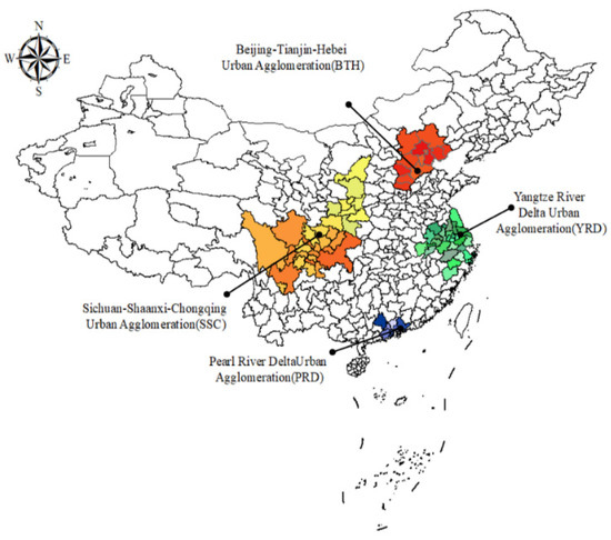
Figure 1.
Location diagram of four major urban agglomerations in China (Ministry of Natural Resources of the People’s Republic of China, 2019).
4.2. Selection of Evaluation Indicators and System Construction
The scientific and reasonable selection of evaluation indicators and the construction of the system play a decisive role in the accuracy of the research results [42]. Considering that there are no accurate statistics of CCL related data in the existing statistical standards, referring to the existing research results and availability of the data, the selection of CCLE evaluation indicators and system construction used in this paper are shown in Table 1. As of March 2023, the 2022 China Energy Statistical Yearbook had not been officially published. Therefore, the most recent year of all statistical yearbooks used in this paper is 2021, with the most recent data being from 2020. The data, spanning from 2010–2020, were extracted from the China Statistical Yearbook (2011–2021), the China Logistics Yearbook (2011–2021), the China Cold Chain Logistics Development Report (2011–2021), and the China Energy Yearbook (2011–2021). In particular, due to the lack of data on the energy consumption of CCL, we used the energy consumption of the logistics industry to calculate the carbon emissions with reference to the methodology of IPCC [43,44], as shown in Equation (7). Then, the value was multiplied by the ratio of the total amount of CCL to the total amount of social logistics in each region to indirectly estimate the carbon emissions of CCL.
where is the total carbon emissions; is the consumption of various forms of energy in the regional CCL, i.e., coal, gasoline, kerosene, diesel, fuel oil, liquefied petroleum gas, and natural gas, respectively; represents the average low calorific value; is the carbon emission coefficient; and is the carbon oxidation factor, which defaults to 1.

Table 1.
Selection of the CCLE evaluation index.
4.3. Data Processing
Based on the system construction and data collection, we preprocessed the data obtained, including performing the homogeneity test, the reduction in the dimension of the input variables, and normalization.
(1) Homogeneity test
Using DEA to measure efficiency, the input and output variables should be isotropic to ensure the scientific validity of the study. We used the Pearson correlation coefficient for the test. The test results are shown in Table 2. It can be seen that the correlation coefficients between the input and output indexes are positive, and more than 90% of the correlation coefficients are greater than 0.6, which is a strong correlation, and all correlation coefficients pass the two-tailed test. These results meet the preconditions of DEA and are suitable for this study.
Table 2.
Homoscedasticity test results for input and output variables from 2010 to 2020.
(2) Dimension reduction of input variables
Due to the large number of input variables in Table 1, the data do not meet the requirements of the DEA model for the number of variables, so the principal component analysis (PCA) method is used for data dimensionality reduction.
The results of the KMO and Bartlett’s tests are shown in Table 3. The analysis of the results shows that the KMO value is 0.825, which is greater than 0.8, and the probability of significance is 0.000, which is less than 0.05, indicating that the data are suitable for PCA.
Table 3.
KMO and Bartlett’s test.
As shown in Table 4, the results reveal that when the three principal components are extracted, the cumulative variance contribution rate is 82.64%, which is greater than 80%, which can better reflect the vast majority of information of the six indicators. Therefore, the three principal components can be substituted into the DEA model as the representatives of input resources.
Table 4.
Eigenvalues and cumulative contributions of PCA.
(3) Normalization processing
Since the new input variables obtained by dimensionality reduction exhibit significant differences from the other variables in terms of magnitude and value, this paper adopted the extreme difference method to standardize the variables [45], which are all values in the range of . The calculation formula is as follows:
where denotes the input and output variables after standardization, respectively; denotes the new input variables obtained by PCA and the original output variables.
5. Results and Analysis
Based on the above theories and methods, in this section we first design static and dynamic measures of CCLE and analyze the overall and regional differences, respectively, in the results; we then apply the Tobit regression model to explore the affective factors of CCLE, laying the theoretical foundation for efficiency improvement strategies.
5.1. Static Measurement of CCLE
Based on a three-stage DEA model, this section solves the comprehensive technical efficiency (TE), pure technical efficiency (PTE), and scale efficiency (SE), and analyzes them from different perspectives.
5.1.1. Comprehensive Analysis
Table 5 shows the CCLE measurement results in the case of carbon emission inclusion/exclusion in the input index.
Table 5.
Results of the efficiency measurement, with and without carbon emissions, from 2010 to 2020.
Whether carbon emission is included in the input variable or not, the TE of the study area exhibits a steady upward trend between 2012 and 2020, which shows that the CCLE has improved in recent years. As shown in Figure 2, when carbon emission is included in the input index, the TE of CCL decreases, and the efficiency, neglecting carbon emission, is overestimated. The figure shows that if investment factors, such as capital, labor, and technology, are exclusively considered, and energy and environmental constraints are ignored, the calculation results are not accurate. Therefore, when constructing the evaluation index system, considering carbon emission is more in line with the actual situation, which also verifies the rationality of the model constructed in this paper.
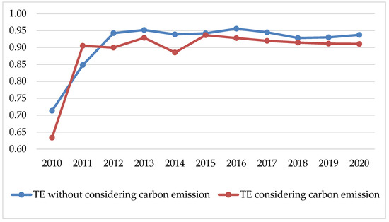
Figure 2.
TE of CCL, determining whether or not to consider carbon emissions.
In addition, the PTE, when considering carbon emission after 2012, is higher than that when carbon emission is not considered. This convincingly shows that the CCL industry is more technologically and managerially advanced when considering energy and environmental constraints. This is because, under the developing trend of energy savings and emissions reduction, the government promotes the CCL industry through policy regulation and other means, while enterprises respond by improving the development and implementation of advanced technologies and promoting management tools to enhance the technology level of the CCL, thus increasing the CCLE.
Although the CCLE considering carbon emission show continuous improvement from 2010 to 2020, there are variations in the trends of TE, PTE, and SE, as demonstrated in Figure 3. The PTE is the closest to the efficiency frontier, remaining at a high level and maintaining an upward trend, indicating a high level of technology and management in the study area as a whole. However, in contrast to the increasing trend in PTE, the trends for combined TE and SE are much closer, both showing an upward trend from 2010 to 2012 and a downward trend after 2013.
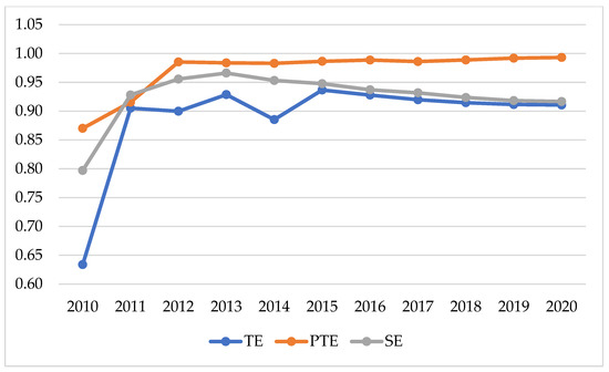
Figure 3.
Average CCLE, considering carbon emission, from 2010 to 2020.
Therefore, for the four urban agglomerations, the common factor restricting the improvement of CCLE is the low SE. Although the improvement in PTE could offset part of the inhibition of SE, the effect is not obvious. The focus of the four urban agglomerations to improve the level of CCL should be to improve the diseconomies of scale and scale efficiency by increasing the scale and optimizing resource allocation.
Due to the differences in regional economic development levels and industrial structures, in order to further analyze the development characteristics and trend of CCL in the four urban agglomerations, the difference analysis of CCL, considering carbon emission, will be carried out below.
5.1.2. Regional Difference Analysis Considering Carbon Emission
The results of the analysis in the previous subsection show that the CCLE, considering carbon emission, is continuously improving from 2010 to 2020, but there are differences between regions in regards to TE, PTE, and SE; therefore, this subsection carries out a regional difference analysis. The results of the CCLE, with carbon emission, in different regions from 2010 to 2020 are shown in Table 6.
Table 6.
Results of the CCLE, with carbon emission, in different regions from 2010 to 2020.
As shown in Figure 4, the PRD has always remained at the forefront of efficiency. It indicates that the development of the CCL industry in the region is relatively green, with low carbon emissions, and is more mature than that in other regions. This may be because fresh agricultural products account for more than 90% of the CCL flows, while the PRD is one of the three major fruit production bases in China, and it is also relatively rich in aquatic resources. The huge scale of the supply of fresh agricultural products has led to the construction and improvement of the infrastructure, which has contributed to the CCLE.
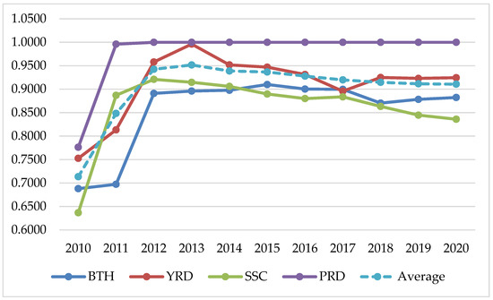
Figure 4.
Average TE of all regions from 2010 to 2020.
From 2011 to 2014, the region with the lowest TE is the BTH, followed by the SSC. The reason may be that Beijing–Tianjin–Hebei integration released in 2015 proposed to “promote the coordinated development of logistics industry”, in which the CCL became a key focus area [46]. The positive policy environment promotes the coordinated development and scale development of CCL in the BTH, and finally, improves efficiency. The SSC is located in the less developed Western Region of China. Compared to other regions, the low level of economic development, the complex geographical environment, and the lack of a perfect layout and infrastructure construction of the CCL restrict the improvement of TE. There is a large gap between the SSC and other regions. Therefore, for the SSC, determining how to narrow the regional gap through reasonable measures is of great significance in improving its own—as well as the overall—CCLE of the whole country.
From the perspective of PTE, the PRD and the YRD were the highest, reaching the efficiency frontier in most years, indicating that these two regions had a high level of logistics technology and management. This region was followed by the SSC, while the BTH has the lowest PTE. In the future, the focus should be on improving pure technical efficiency and striving to improve the technical and management levels in the area.
In terms of SE, the PRD remained at the frontier of efficiency, while the YRD was closer to the average. Taking 2012 as the time point, the SE of the BTH was the lowest in the first period, and the SE of the SSC was the lowest, demonstrating a downward trend. Therefore, for the SSC, in the future, efforts should be made to promote factor agglomeration and industrial synergy development to improve SE.
5.2. Dynamic Measurement of CCLE
To gain a deeper understanding of the dynamic changes in regional CCLE from a low-carbon perspective, this subsection utilizes input-output data obtained from the three-stage DEA analysis and applies the Malmquist index model to obtain the TFP index and its decomposition for each region under carbon constraints. On the basis of these results, we conduct an analysis of the overall and variances of the dynamic changes in CCLE.
5.2.1. Global Analysis
Table 7 presents the mean value and decomposition results of the TFP index of CCL in the study area, under carbon constraints, from 2010 to 2020.
Table 7.
TFP index and decomposition results of overall CCL under carbon constraint.
The results indicate that from 2011 to 2020, the Malmquist index for the study area remained above 1, suggesting an overall upward trend in the TFP of CCL, when taking carbon emissions into account. The average annual growth rate was 1.25%, with techch contributing the most significantly, with an average annual growth rate of 4.20%. This can be attributed to advancements in technology. Additionally, the strong growth in demand for CCL was fueled by China’s rapid economic development and the emergence of new industrial models, such as e-commerce, during this period. At the same time, the introduction of relevant positive policies, such as Logistics Industry Adjustment and Revitalization Planning [47] and the Medium and Long Term Plan for the Development of the Logistics Industry (2014–2020) [48], during the period has prompted a clear trend of technological innovation and energy savings, along with low-carbon trends, in the CCL industry. While promoting the overall CCLE, each region also pays great attention to energy and environmental constraints.
5.2.2. Variance Analysis
Table 8 shows the TFP of the CCL and its decomposition results for each urban ag-glomeration. When considering regional differences, the highest TFP of CCL under carbon constraints is found in the PRD, followed by the YRD and BTH, with all of them exceeding 1. On the contrary, the SSC exhibits the lowest TFP, which is less than 1 and significantly lower than that of other urban agglomerations.
Table 8.
TFP index and decomposition results of CCL in four urban agglomerations, under carbon constraint.
In addition, the YRD exhibits the highest techch, while the BTH has the highest pech, and the PRD shows the highest effch and sech. The relatively stable technical efficiency and scale efficiency across regions are important factors contributing to the high-quality development of CCL. In contrast, the SSC shows less satisfactory indicators. Combined with the results in Section 5.1 showing the static measurement of CCLE in each region, it can be observed that the CCLE in the SSC region increases over the study period, but there is a 2% decrease in TFP, which can be attributed to the simultaneous decline of TE and SE. Therefore, for the SSC, it is not only necessary to continue to strengthen the infrastructure construction and expand the scale of CCL but also to continuously promote technological innovation and progress in the field of CCL under the background of green and low-carbon development.
5.3. The Influencing Factors of CCLE
The results of both static and dynamic CCLE measurements indicate that although the overall level of CCL development in each urban agglomeration has improved, significant differences still exist. Therefore, improvement strategies should be targeted accordingly. Building on the aforementioned research, this subsection investigates the influencing factors of CCLE and analyzes the direction and extent of each factor’s impact, providing a theoretical foundation for the formulation of improvement strategies.
Among the available research results, scholars have mainly considered the influence of factors such as the level of economic development, economic structure, and industrial agglomeration on the CCLE. To ensure the rationality of index selection and data availability, we developed an index system of influencing factors, as described in Table 9.
Table 9.
Index system of CCLE influencing factors.
We selected four influential factors, including the level of economic development (EL), the degree of openness to the outside world (OD), the energy structure (ES), and government intervention (GD), as explanatory variables. To construct a Tobit regression model, we used CCLE, under carbon constraints, obtained from the three-stage DEA model–Malmquist index model as the dependent variable. After the Hausman test, the index system was further determined as a panel Tobit random effect regression model, which is shown in Equation (9), where is the constant, are the regression parameters of each index, respectively, and is the residual error. The results are shown in Table 10, indicating that all variables pass the significance test, and the goodness of fit of the data is good.
Table 10.
Tobit regression results of influencing factors of CCLE (regression coefficient).
Specifically, the impact coefficients of all indicators of the CCLE in the BTH region are positive. The coefficient of EL is the highest at 0.8094, which is consistent with the expectations that economic development can effectively promote the development of the CCL industry. This is because economic progress is often accompanied by phenomena such as the upgrading of industrial structures, the introduction of advanced technologies, and the gathering of capital and outstanding talents, which all play a positive role in promoting the CCL.
In the YRD, the influence coefficients of EL, OD, and GD are positive, while only the ES is negative, with an influence coefficient of −0.3667, indicating that the main factor restricting the development of CCL in the YRD at present is the unreasonable energy structure. This means that more energy input would lead to a decrease in the CCLE. This indicates that although the scale and service level of CCL in the YRD are expanding, the environmental impact of high energy consumption is becoming increasingly severe, resulting in significant ecological costs. Therefore, it is necessary to prioritize the promotion of the sustainable development of CCL by adopting a low-carbon approach to energy and improving the cleanliness of current energy sources.
In the SSC, both OD and GD show a significant negative effect, and the latter has a greater effect, with the influence coefficients of −0.7421 and −0.8431, respectively. From the perspective of OD, the SSC is located in the Western Inland Region of China, with a complex geographical environment and poor transportation accessibility. Therefore, the low degree of openness to the outside world has affected the development of CCL. In terms of the GD, national strategies such as China’s Western Region Development Strategy could play a positive role in the development of this area [49]. However, the logistics infrastructure construction in the urban agglomeration of SSC is weak, and the government’s support for the industry is insufficient, while competition exists between regions within the urban agglomeration. Hence, unreasonable government intervention may, to a certain extent, instead intensify resource competition and cause phenomena such as unreasonable resource allocation, which is not conducive to the development of CCL. The SSC should focus on expanding the degree of openness to the outside world and increasing the intensity and rationality of government intervention.
The impact of different factors in the PRD is similar to that in the YRD. Specifically, the EL, OD, and GD have a positive effect, while the ES has a negative impact. This suggests that the PRD’s energy structure also requires improvement.
6. Conclusions and Implications
6.1. Conclusions
This study applies the three-stage DEA and Malmquist index model to statically and dynamically evaluate the CCLE of China’s four primary urban agglomerations (BTH, YRD, PRD, and SSC) during the period between 2010 and 2020, from a low-carbon perspective. The Tobit regression model is employed to identify the main factors that contribute to the enhancement of CCLE. The main conclusions are as follows.
Firstly, during the period of 2010–2020, the CCLE in the study area shows an overall upward trend under both the carbon constraint and non-carbon constraint scenarios, indicating an improvement in the development level of CCL. However, there are significant differences in each region under the two different situations, implying that environmental regulation could affect the development of CCL. Therefore, improving CCLE and implementing energy conservation and emission reduction should become the primary development goals in the future.
Secondly, the CCLE of the PRD is always the closest to the efficiency frontier, from a static perspective, followed by the YRD, indicating that their expansion is in good condition and that they can continue to maintain the development trend. The main factors limiting the CCLE in the BTH and SSC are PTE and SE, respectively. From a dynamic point of view, the TFP of CCL in all regions has increased from 2010 to 2020, with the main driving factor being the improvement in technological change. However, attention should be paid to the TFP of the CCL in the SSC, which is less than 1.
Finally, in terms of influencing factors, EL, OD, ES, and GD all have an impact on the CCLE, but the direction and degree of influence of each factor differ in various regions. EL has promoted CCLE in all regions, but the impact coefficient of ES is negative for YRD and PRD. OD and GD also have a negative impact on CCLE in the SSC.
6.2. Implications
Based on the above findings, this study proposes several insights to promote the low-carbon, efficient, and balanced development of cold chain logistics.
Firstly, there is a need to improve the research and development of key technologies and advanced equipment in the cold chain logistics sector, aiming to improve the energy-saving capabilities of cold chain logistics facilities and equipment. Green and low-carbon production has become the inevitable trend of the development of cold chain logistics [50]. The government should recognize the significance of technological progress and innovation in enhancing CCLE and actively improve the application of technologies such as big data, 5G, blockchain technology, and artificial intelligence in the field of cold chain logistics. It should also expedite the replacement of highly polluting refrigerated lorries and encourage the exploration and development of small and lightweight modern refrigerated lorries and containers to accelerate the pace of emission reduction and the low-carbon transformation of cold chain logistics.
Secondly, advanced regions should play a demonstrative and leading role in promoting and driving the collaborative and large-scale development of cold chain logistics. The study finds that the CCLE of the four urban agglomerations is significantly different, and low-scale efficiency is one of the important factors restricting their CCLE. Therefore, it is essential to fully utilize the high CCLE urban agglomeration’s demonstrative role and steer the cluster development of cold chain logistics components by adjusting the industrial scale, consolidating logistics resources, coordinating regional advancement, strengthening facility linkage and information connectivity, in order to enhance the scale level of cold chain logistics.
Finally, the government should reasonably formulate guidance policies related to the development of cold chain logistics. Taking into account the actual development of the region, the government should actively play a guiding and regulating role, make use of the situation, identify the focus point of the policy, exert precise efforts, and comprehensively formulate the strategy or implementation plan for the development of cold chain logistics in the region in order to systematically promote the high-quality development of cold chain logistics in different regions. For example, all urban clusters should mainly concentrate on improving the level of economic development to promote the expansion of the regional cold chain logistics market and the improvement of infrastructure facilities, which in turn will promote the improvement of CCLE. The YRD and PRD also need to concentrate on the energy structure and promote the adoption of natural cold energy, solar energy, and other eco-friendly energy sources.
6.3. Limitations
This paper contributes to the enrichment and enhancement of the CCLE evaluation methodology, offering a theoretical foundation for advancing CCLE improvement and sustainable development. Nevertheless, it is important to acknowledge certain limitations. Due to the limited availability of the data, the empirical study only covers the period from 2010 to 2020. Additionally, the selection of evaluation indicators is somewhat narrow due to the limited availability of information such as statistical yearbooks. In the future, if there is more comprehensive data support, additional research and analysis should be carried out using a longer time perspective and a richer indicator system. Secondly, in the future, the results should be compared with those of other studies to enhance their reliability and validity. Finally, a quantitative evaluation of measures to promote CCLE can be considered to provide a basis for relevant government departments to formulate more effective policies.
Author Contributions
Conceptualization, M.H.; methodology, M.H. and M.Y.; software, M.Y.; validation, M.H., M.Y., X.W. and J.P.; formal analysis, M.Y. and X.W.; investigation, J.P.; data curation, X.W.; writing—original draft preparation, M.H., M.Y. and X.W.; writing—review and editing, J.P.; visualization, J.P.; supervision, K.I.; project administration, M.H.; funding acquisition, X.W. All authors have read and agreed to the published version of the manuscript.
Funding
This research was funded by the Humanity and Social Science Youth Foundation of the Ministry of Education of China (grant number No. 21YJCZH180), the Research Foundation of Philosophy and Social Sciences in the Universities of Jiangsu Province, China (grant number No. 2020SJA2058), and the Research Innovation Program for Postgraduates of General Universities in Jiangsu Province (grant number No. KYCX22_3674).
Institutional Review Board Statement
Not applicable.
Informed Consent Statement
Not applicable.
Data Availability Statement
The data presented in this study are available on request from the corresponding author.
Conflicts of Interest
The authors declare no conflicts of interest.
References
- Guo, X.; Zhang, W.; Liu, B. Low-carbon routing for cold-chain logistics considering the time-dependent effects of traffic congestion. Transp. Res. Part D-Transp. Environ. 2022, 113, 103502. [Google Scholar] [CrossRef]
- Wang, H.; Liu, W.; Liang, Y. Measurement of CO2 Emissions Efficiency and Analysis of Influencing Factors of the Logistics Industry in Nine Coastal Provinces of China. Sustainability 2023, 15, 14423. [Google Scholar] [CrossRef]
- IEA. CO2 Emissions in 2022; IEA: Paris, France, 2023. [Google Scholar]
- State Council of China. Opinions on the Complete, Accurate and Comprehensive Implementation of the New Development Concept to Do a Good Job of Carbon Peaking and Carbon Neutral Work. 2021. Available online: https://www.gov.cn/zhengce/2021-10/24/content_5644613.htm (accessed on 20 August 2022). (In Chinese)
- Leng, L.; Wang, Z.; Zhao, Y.; Zuo, Q. Formulation and heuristic method for urban cold-chain logistics systems with path flexibility—The case of China. Expert Syst. Appl. 2024, 244, 122926. [Google Scholar] [CrossRef]
- Li, D.; Li, K. A multi-objective model for cold chain logistics considering customer satisfaction. Alex. Eng. J. 2023, 67, 513–523. [Google Scholar] [CrossRef]
- Zhang, N.; Zhou, P.; Kung, C. Total-factor carbon emission performance of the Chinese transportation industry: A bootstrapped non-radial Malmquist index analysis. Renew. Sustain. Energy Rev. 2015, 41, 584–593. [Google Scholar] [CrossRef]
- State Council of China. The “14th Five-Year Plan” for the Development of Cold Chain Logistics. 2021. Available online: https://www.gov.cn/zhengce/content/2021-12/12/content_5660244.htm (accessed on 15 June 2022). (In Chinese)
- Fugate, B.S.; Mentzer, J.T.; Stank, T.P. Logistics Performance: Efficiency, Effectiveness, and Differentiation. J. Bus. Logist. 2010, 31, 43–62. [Google Scholar] [CrossRef]
- Park, H.G.; Lee, Y.J. The Efficiency and Productivity Analysis of Large Logistics Providers Services in Korea. Asian J. Shipp. Logist. 2015, 31, 469–476. [Google Scholar] [CrossRef]
- Hammes, G.; De Souza, E.D.; Rodriguez, C.M.T.; Millan, R.H.R.; Herazo, J.C.M. Evaluation of the reverse logistics performance in civil construction. J. Clean. Prod. 2020, 248, 119212. [Google Scholar] [CrossRef]
- Cavaignac, L.; Dumas, A.; Petiot, R. Third-party logistics efficiency: An innovative two-stage DEA analysis of the French market. Int. J. Logist.-Res. Appl. 2021, 24, 581–604. [Google Scholar] [CrossRef]
- Liang, Z.; Chiu, Y.; Guo, Q.; Liang, Z. Low-carbon logistics efficiency: Analysis on the statistical data of the logistics industry of 13 cities in Jiangsu Province, China. Res. Transp. Bus. Manag. 2022, 43, 100740. [Google Scholar] [CrossRef]
- Barilla, D.; Carlucci, F.; Cirà, A.; Ioppolo, G.; Siviero, L. Total factor logistics productivity: A spatial approach to the Italian regions. Transp. Res. Part A-Policy Pract. 2020, 136, 205–222. [Google Scholar] [CrossRef]
- Cao, B.; Kong, Z.; Deng, L. Evolution of Time and Space Efficiency of Provincial Logistics in the Yangtze River Economic Belt. Sci. Geogr. Sin. 2019, 39, 1841–1848. [Google Scholar] [CrossRef]
- Chang, K.; Wan, Q.; Lou, Q.; Chen, Y.; Wang, W. Green fiscal policy and firms’ investment efficiency: New insights into firm-level panel data from the renewable energy industry in China. Renew. Energy 2020, 151, 589–597. [Google Scholar] [CrossRef]
- Yu, J.; Zhou, K.; Yang, S. Regional heterogeneity of China’s energy efficiency in “new normal”: A meta-frontier Super-SBM analysis. Energy Policy 2019, 134, 110941. [Google Scholar] [CrossRef]
- Yu, X.; Xu, H.; Lou, W.; Xu, X.; Shi, V. Examining energy eco-efficiency in China’s logistics industry. Int. J. Prod. Econ. 2023, 258, 108797. [Google Scholar] [CrossRef]
- Sueyoshi, T.; Goto, M. DEA environmental assessment in time horizon: Radial approach for Malmquist index measurement on petroleum companies. Energy Econ. 2015, 51, 329–345. [Google Scholar] [CrossRef]
- Jiang, X.; Ma, J.; Zhu, H.; Guo, X.; Huang, Z. Evaluating the Carbon Emissions Efficiency of the Logistics Industry Based on a Super-SBM Model and the Malmquist Index from a Strong Transportation Strategy Perspective in China. Int. J. Environ. Res. Public Health 2020, 17, 8459. [Google Scholar] [CrossRef] [PubMed]
- Lan, S.; Tseng, M.; Yang, C.; Huisingh, D. Trends in sustainable logistics in major cities in China. Sci. Total Environ. 2020, 712, 136381. [Google Scholar] [CrossRef]
- Lo Storto, C.; Evangelista, P. Infrastructure efficiency, logistics quality and environmental impact of land logistics systems in the EU: A DEA-based dynamic mapping. Res. Transp. Bus. Manag. 2023, 46, 100814. [Google Scholar] [CrossRef]
- Chen, W.; Pan, Y. Logistics Industry Total Factor Productivity Spatial Differentiation and Space-time Evolution at Low Carbon Constraints. J. Ind. Technol. Econ. 2016, 35, 42–52. [Google Scholar] [CrossRef]
- Yu, M.; Lee, J.Y. Polydeoxyribonucleotide improves wound healing of fractional laser resurfacing in rat model. J. Cosmet. Laser Ther. 2017, 19, 43–48. [Google Scholar] [CrossRef] [PubMed]
- Xin, Y.; Zheng, K.; Zhou, Y.; Han, Y.; Tadikamalla, P.R.; Fan, Q. Logistics Efficiency under Carbon Constraints Based on a Super SBM Model with Undesirable Output: Empirical Evidence from China’s Logistics Industry. Sustainability 2022, 14, 5142. [Google Scholar] [CrossRef]
- Wu, F.; Zhu, X. Cold Chain Logistics Network Optimization Model Based on Hub-and-Spoke Theory. J. Highw. Transp. Res. Dev. 2019, 36, 144–150. [Google Scholar]
- Yu, Q.; Yang, Y.; Huang, R. Study on the Node Location Optimization of Fresh Agricultural Products International Cold Chain Logistics Network under the One Belt One Road Strategy. Logist. Eng. Manag. 2017, 39, 1–5. [Google Scholar] [CrossRef]
- Li, G. Development of cold chain logistics transportation system based on 5G network and Internet of things system. Microprocess. Microsyst. 2021, 80, 103565. [Google Scholar] [CrossRef]
- Yan, L.; Grifoll, M.; Zheng, P. Model and Algorithm of Two-Stage Distribution Location Routing with Hard Time Window for City Cold-Chain Logistics. Appl. Sci. 2020, 10, 2564. [Google Scholar] [CrossRef]
- Zhang, Y.; Hua, G.; Cheng, T.C.E.; Zhang, J. Cold chain distribution: How to deal with node and arc time windows? Ann. Oper. Res. 2020, 291, 1127–1151. [Google Scholar] [CrossRef]
- Shi, Y.; Lin, Y.; Lim, M.K.; Tseng, M.; Tan, C.; Li, Y. An intelligent green scheduling system for sustainable cold chain logistics. Expert Syst. Appl. 2022, 209, 118378. [Google Scholar] [CrossRef]
- Fried, H.O.; Lovell, C.A.K.; Schmidt, S.S.; Yaisawarng, S. Accounting for Environmental Effects and Statistical Noise in Data Envelopment Analysis. J. Prod. Anal. 2002, 17, 157–174. [Google Scholar] [CrossRef]
- Luo, D. A Note on Estimating Managerial Inefficiency of Three-Stage DEA Model. Stat. Res. 2012, 29, 104–107. [Google Scholar] [CrossRef]
- Chen, W.; Zhang, L.; Ma, T.; Liu, Q. Research on Three-stage DEA Model. Syst. Eng. 2014, 32, 144–149. [Google Scholar] [CrossRef]
- Grammatikopoulou, I.; Sylla, M.; Zoumides, C. Economic evaluation of green water in cereal crop production: A production function approach. Water Resour. Econ. 2020, 29, 100148. [Google Scholar] [CrossRef]
- Zheng, Z. Energy efficiency evaluation model based on DEA-SBM-Malmquist index. Energy Rep. 2021, 7, 397–409. [Google Scholar] [CrossRef]
- Bansal, P.; Kumar, S.; Mehra, A.; Gulati, R. Developing two dynamic Malmquist-Luenberger productivity indices: An illustrated application for assessing productivity performance of Indian banks. Omega-Int. J. Manag. Sci. 2022, 107, 102538. [Google Scholar] [CrossRef]
- Xue, L.; Zhao, S. Evaluating and Analyzing the Operation Efficiency of Urban Rail Transit Systems in China Using an Integrated Approach of DEA Model, Malmquist Productivity Index, and Tobit Regression Model. J. Transp. Eng. Part A-Syst. 2021, 147, 4021061. [Google Scholar] [CrossRef]
- Tobin, J. Estimation of Relationships for Limited Dependent Variables. Econometrica 1958, 26, 24–36. [Google Scholar] [CrossRef]
- Zhu, C.; Zhu, N.; Shan, W.U.H.; Cunkas, M. Eco-Efficiency of Industrial Investment and Its Influencing Factors in China Based on a New SeUo-SBM-DEA Model and Tobit Regression. Math. Probl. Eng. 2021, 2021, 5329714. [Google Scholar] [CrossRef]
- Yang, L.; Liang, Z.; Yao, W.; Zhu, H.; Zeng, L.; Zhao, Z. What Are the Impacts of Urbanisation on Carbon Emissions Efficiency? Evidence from Western China. Land 2023, 12, 1707. [Google Scholar] [CrossRef]
- Liu, W.; Wang, S.; Dong, D.; Wang, J. Evaluation of the intelligent logistics eco-index: Evidence from China. J. Clean. Prod. 2020, 274, 123127. [Google Scholar] [CrossRef]
- IPCC. IPCC Guidelines for National Greenhouse Gas Inventories; Institute for Global Environmental Strategies (IGES): Hayama, Japan, 2006. [Google Scholar]
- IPCC. The 2019 Refinement to the 2006 IPCC Guidelines for National Greenhouse Gas Inventories; Task Force on National Greenhouse Gas Inventories (TFI): Kyoto, Japan, 2019. [Google Scholar]
- Chong, Y.; Chen, N.; Weng, S.; Xu, Z. Regional Sustainability of Logistics Efficiency in China along the Belt and Road Initiative Considering Carbon Emissions. Sustainability 2022, 14, 9506. [Google Scholar] [CrossRef]
- National Development and Reform Commission of China. Circular of the National Development and Reform Commission on Accelerating the Implementation of Major Modern Logistics Projects. 2015. Available online: https://www.ndrc.gov.cn/fggz/jjmy/ltyfz/201508/t20150813_1121080.html?code=&state=123 (accessed on 20 December 2021). (In Chinese)
- State Council of China. Action Plan for Carbon Dioxide Peaking before 2030. 2015. Available online: http://www.gov.cn/zhengce/content/2021-10/26/content_5644984.htm (accessed on 30 October 2021). (In Chinese)
- State Council of China. The Medium and Long Term Plan for the Development of the Logistics Industry (2014–2020). 2014. Available online: http://www.gov.cn/zhengce/content/2014-10/04/content_9120.htm (accessed on 12 September 2021). (In Chinese)
- China Development Gateway. The Revitalisation of Western China. 2021. Available online: http://cn.chinagate.cn/economics/node_2364447.htm (accessed on 15 December 2021). (In Chinese).
- Han, J.; Zuo, M.; Zhu, W.; Zuo, J.; Lü, E.; Yang, X. A comprehensive review of cold chain logistics for fresh agricultural products: Current status, challenges, and future trends. Trends Food Sci. Technol. 2021, 109, 536–551. [Google Scholar] [CrossRef]
Disclaimer/Publisher’s Note: The statements, opinions and data contained in all publications are solely those of the individual author(s) and contributor(s) and not of MDPI and/or the editor(s). MDPI and/or the editor(s) disclaim responsibility for any injury to people or property resulting from any ideas, methods, instructions or products referred to in the content. |
© 2024 by the authors. Licensee MDPI, Basel, Switzerland. This article is an open access article distributed under the terms and conditions of the Creative Commons Attribution (CC BY) license (https://creativecommons.org/licenses/by/4.0/).