1. Introduction
Intensive precipitation events and the resulting soil erosion and sediment transport are a global problem that leads to disruption of landscape processes and degradation of arable land and water resources [
1]. Although soil erosion and sediment transport are mainly natural processes, human use of the landscape, especially through unsustainable agricultural activities, accelerates the whole process, including the severity of the consequences [
2]. Excessive erosion can also cause extensive damage to community infrastructure and even directly endanger the lives of residents [
3]. More than 20% of agricultural land in over a third of OECD member countries is at risk of moderate to severe erosion [
4]. Worldwide, up to 30% of agricultural land is threatened by erosion due to the intensification of agriculture, and, among other consequences, erosion intensively threatens food production [
5,
6,
7].
Excessive soil erosion on the land and in-stream channel erosion are global problems impacting the sustainability of the world’s water resources [
8,
9]. Central Europe experiences impacts from sediments transported from agricultural land, leading to damage in water courses and water bodies and damage to infrastructure in urban areas [
10]. Furthermore, in the central and southern parts of the United States (including the Oostanaula Creek watershed), bank erosion is thought to contribute significantly (if not critically) to the overall transport of erosional sediments [
11]. As can be seen, it is no longer sustainable to exploit the landscape and overlook the consequences of human activities [
12]. Thanks to research activities, the causes and consequences of soil loss have been known for decades, but due to the rapid development of industrial society and technologies, the consequences are often ignored and underestimated because agricultural profit is the priority [
13].
Another environmental factor further worsening the situation and deepening the conflicts of interest between the environment, people, the economy, and society is global climate change [
14]. One of the studies predicts worsening soil erosion rates by up to 10% in the next 50 years due to climate change [
15]. The global climate is changing dramatically and even faster than expected. It influences the distribution of precipitation (in some places) and the amount of precipitation and also changes the kinetic energy. One of the changing factors that is often neglected is the change in crop rotation in response to climate change or even the development of new crop varieties that affect the economic profit of the current market depending on the political situation [
16].
Researchers observing and predicting climate change, coupled with further land development impacting our society, need to take action by effectively communicating, explaining, and disseminating information. An appropriate avenue for this is to outline the ongoing search for sustainable, socially acceptable solutions (measures) to reduce soil loss, sediments, and water pollution caused by factors such as bound nutrients and pesticides. This effort involves compiling information from the research literature and translating it into a format suitable for diverse audiences, including farmers, associations, competent authorities and the general public. The process includes describing the current environmental condition, identifying high-risk factors and areas, and testing various scenarios to understand potential model outcomes.
To model and assess the risk of severe erosion for a specific location, researchers can employ erosion and transport models to determine the soil loss or erosion intensity on the land or in the watershed. In general, models can be divided into empirical-statistical, conceptual, and physical models [
17]. Models differ, on the one hand, in the required quality and quantity of inputs and, on the other hand, in the resulting quality and representativeness of the delivered results. The interannual yield of sediments, applied in reservoirs, was solved by using probabilistic erosion models [
18]. For ungauged catchments, a mathematical model can be used to estimate erosion, as in the work of Hrissanthou [
19].
Empirical models based on the principle of the Universal Soil Loss Equation (USLE) are generally used to determine the erosion risk in large areas with an acceptable amount and detail of inputs. The USLE determines the long-term average soil loss in a catchment caused by sheet erosion. One such model is the spatially distributed WaTEM/SEDEM model [
20,
21,
22], which provides a sufficiently accurate estimate of erosion intensity and transported eroded material based on a relatively small amount of input data [
23]. Based on the global review of the most commonly used models for predicting soil erosion and sediment yields, the WaTEM/SEDEM model is within the top five with RUSLE, USLE, WEPP, and SWAT [
24]. This model has been extensively tested and used to determine sediment transport and sedimentation in reservoirs under conditions in the Czech Republic [
25,
26,
27] as well as worldwide [
28,
29].
Land use is one of the critical inputs for watershed models that significantly influences the accuracy of erosion and sediment transport [
10]. In general, the degree of the ability to control the land use layer quality is proportional to the size of the modeled area. For extensive areas, it is very time-consuming to perform targeted surveys to verify the accuracy of the input data. Nowadays, there are various satellite products that offer commercial or freely available land use data suitable for modeling. The Landsat program has the longest history, and its products are available both worldwide and regionally. In the US, the Global Land Cover dataset or the NLCD (National Land Cover Database) have been widely used [
30,
31], publicly available in 30 m resolution.
In Europe, the Corine Land Cover database has mostly been used in recent research [
32]. Based on the Sentinel-2 satellite family, the European Space Agency recently developed the ESA WorldCover dataset in a much better spatial resolution of 10 m [
33]. These recent advances make it possible to improve the input data worldwide, especially in regions where no other detailed land use product is available. In Europe in particular, detailed vector-based land use data for individual agricultural parcels are available as Land Parcel Identification System (LPIS). It was developed by the EU countries to control the compliance of farmers for subsidies and is generally available for any type of public or research use. In the US, there is no such publicly available detailed source that could be used. A particular focus of the indicated measures can be placed on buffer strips along watercourses to enhance trapping efficiency, initiate sediment deposition, and reduce water pollution. Such measures can contribute significantly to water protection [
34]. Since the output of sediment yields from watershed models is highly dependent on accurate spatial land cover data, there is a critical need to better understand how potential land cover inaccuracies affect model outputs.
This manuscript presents a case study targeting a catchment in the Oostanaula Creek watershed located in the state of Tennessee. Within the presented work, the importance of land use data input was assessed to answer the following questions:
1. How significant is the influence of the land use input dataset in terms of modeled sediment inputs into watercourses?
2. Are generally available datasets of land use of sufficient quality to define high-risk locations in terms of erosion? Can they be reliably utilized for assessment without in situ validation of land use datasets?
3. Is it possible to define the probable contribution of channel erosion to the total transport of sediment from the catchment by combining erosion modeling in the catchment and field survey of the hydrologic network?
2. Materials and Methods
The presented case study has been prepared for a catchment within the Oostanaula Creek watershed, where a mathematical model of soil erosion and sediment transport, the WaTEM/SEDEM model [
20,
21,
22], was used to assess the impact of alternative input data sources and to determine critical profiles concerning sediment input and transport.
2.1. Oostanaula Creek Watershed Study Site
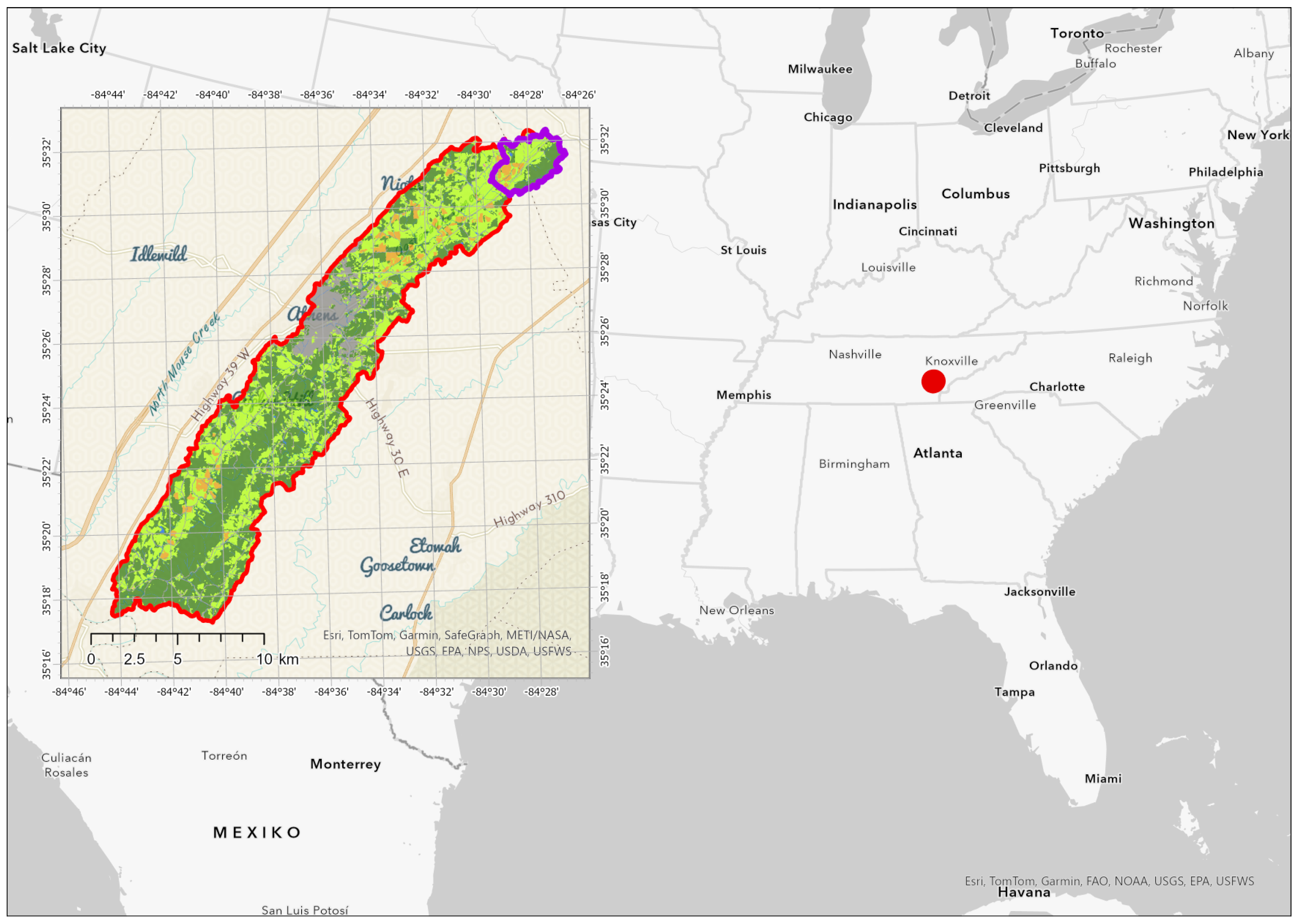
The Oostanaula Creek catchment (
Figure 1) is located in southeast Tennessee (tributary of the Hiwassee River). The area covered by modeling is 182.1 km
2 of the Oostanaula Creek watershed—OCW (HUC 06020021101 and 060200021102).
Oostanaula Creek is typical of streams within the Ridge-and-Valley region of the eastern United States. Annual precipitation ranges from 1100 to 1400 mm. Average summer temperatures range from 19 to 30 °C, and January temperatures range from −3 to 7 °C. Elevations in the OCW range from 240 to 340 m above sea level. The lowest point is in the southwestern part of the watershed at Calhoun, where Oostanaula Creek flows into the Hiwassee River and Chickamauga Lake. This location is about 210 m above sea level [
35].
A total of 323 km of streams (280 km natural and 43 km artificially stabilized) was included in the model in the land area covered by the following land use: forest (46%), grassland (38%), urban areas (12%), and arable lands (4%). The part of the catchment above the city of Athens, Tennessee, is dominated by agricultural use (cultivated crops/pasture), compared with the lower part of the catchment, which is covered mostly by forest. The outlet profile of the entire Oostanaula Creek watershed is located near the town of Calhoun, where Oostanaula Creek flows into the Hiwassee River.
Termed the “Oostanaula-Top”, it is a sub-catchment (9.4 km
2) that was later identified as the research focus, consisting of field surveys, detailed calculations, and model tests (
Figure 1—purple outline). The outlet point of the sub-catchment was established under the County Road 350 bridge crossing Oostanaula Creek (5.3 km of river length). The land use of the Oostanaula-Top part of the catchment is mainly covered by forest (41%), grassland (44%), arable lands (10%), and urban areas (3%). All abovementioned land uses are based on the National Land Cover Database 2016 (NLCD) [
30].
2.2. Model WaTEM/SEDEM Inputs and Parameters
The WaTEM/SEDEM model [
20,
21,
22] is an erosion and transport model based on a simple empirical equation considering six factors based on the USLE method [
36]. The six factors include the rainfall erosivity factor (R); the slope length and slope factors (LS); the vegetation cover and tillage factor (C); the soil erodibility factor (K); and the erosion protection factor (P). The contributing area for the LS calculation is defined by the multiple flow algorithm for splitting the runoff into several streams (directions) [
37]. The full functionality of the model deals with sediment transport—firstly, calculating distributed soil loss; secondly, calculating sediment transport using the transport capacity equation for each element (pixel); and finally, estimating the volume of sediment reaching the river network segments and summarizing the volume leaving the catchment annually (final river segment). The original USLE approach only estimates the potential soil erosion, while the WaTEM/SEDEM model calculates the transport capacity potential in each pixel and then determines the erosion/deposition and potential of the sediment transported from each pixel. The WaTEM/SEDEM model 2.1.0. version was used. For successful calculations, at least these spatially distributed inputs are required: digital elevation model (DEM), land use, and USLE factors (R—rainfall, K—soils, C—vegetation). To determine the sediment load in rivers, the topology of the river (river section) must also be prepared with the correct orientation and linkage. The possibility of sediment deposition in ponds was not relevant for the study and was not considered.
The DEM is based on a tiled collection of the 3D Elevation Program (3DEP) and has a resolution of 1/3 arc second (approximately 10 m) [
38]. The 3DEP dataset serves as the elevation layer of the national map and provides basic elevation information for Earth science studies and mapping applications in the United States. Scientists and resource managers use 3DEP data for hydrologic modeling, resource monitoring, mapping and visualization, and many other applications. The elevations in this DEM represent the topographic surface of the bare Earth.
The R-factor used in this study was set at 4000 MJ·mm·ha
−1·h
−1·yr
−1, based on a revised R-factor study published [
39] with values very close to those originally known from RUSLE [
40]. Tennessee is the sixth rainiest state in the United States according to a recent analysis of monthly and annual precipitation in each state, with an average annual precipitation of 1310 mm.
The K-factor was derived from the “STATSGGO” soil database. This nationwide STATSGO soil database was provided by the National Resources Conservation Service (NRCS). K-factor values were estimated directly based on the known distribution of soil units. K-factor values vary from 0.21 to 0.58 with the mean value of 0.28 (±0.02) in the entire watershed. In the Oostanaula-Top catchment, the min and max K-factor is the same range as the entire watershed, 0.21 to 0.58, and the average value is nearly the same, 0.27 (±0.04).
Data acquisition for the C-, LS-, and P-factors is described next. The C-factor was determined based on information from local farmers. The crop rotation consists of soybeans and maize, mainly using shallow, minimum tillage agrotechnology. The C-factor was set at 0.3 for arable land, 0.01 for grassland, and 0 for all other (non-erosive) types of land use. Due to the focus of the study, which compares the influence of variable factors, the C-factor was used equally in all scenarios. The LS factor is calculated as a routine of the WaTEM/SEDEM model based on the set calculation parameters. The LS and Nearing slope exponent from McCool [
41] were used. The P-factor remains at 1 as no soil protection measures/strategies are applied.
Final model parameters setup for all modeled scenarios are based on previous calibration and usage [
25,
26,
27]: Ktc (Low) = 35, Ktc (High) = 55, Ktc (Limit) = 0.1; Ptef (Cropland) = 0, Ptef (Forest, Pasture) = 75; and Parcel Connectivity (Cropland) = 40, Parcel Connectivity (Forest, Pasture) = 75, model parameters LS and Nearing slope exponent used by McCool [
41], where the Ktc values are transport capacity coefficients, Ptef is a parameter dealing with parcel trapping efficiency by reducing drainage area based on land use coverage, and the Parcel Connectivity parameter issues the boundary effect of the single parcels. More detailed information is provided in documentation of the model published [
21] and available online on the model website.
2.3. Preliminary Investigation of Land Use Datasets for WaTEM/SEDEM Model Input
Two land use datasets were obtained for use in the WaTEM/SEDEM model; they were the National Land Cover Database (NLCD) and the ESA WorldCover dataset. The NLCD is an operational land cover monitoring program providing updated land cover and related information for the United States at five-year intervals. The NLCD2016 extends temporal coverage to 15 years (2001–2016) and was published in 2019. The NLCD is a widely recognized and widely utilized database [
30]. The ESA WorldCover dataset is a newly available worldwide data source in better spatial and temporal resolution (10 m), published in late 2022 based on Sentinel-2 and Sentinel-1 satellite images, reaching overall accuracy of 77% and independently validated [
33].
Initially, the main purpose of the study was to use the NLCD, a publicly available and commonly used dataset across the United States supplying land use input data for the WaTEM/SEDEM model, and use that data for identifying problematic areas. Data were also used to build model scenarios of conservation areas through the installation of grass buffer strips along watercourses and ultimately to evaluate the improvements from protective practices. During the initial model development, substantial discrepancies were found between the source of land use data (NLCD, 30 m resolution) and visible observations from orthophoto aerial images, which appeared to strongly influence the model results.
Fortunately, to improve the land cover dataset, the ESA WorldCover dataset was available as an alternative data source for the study’s model. At the same time, a manual dataset of land use was created directly onsite through field measurements using imagery from an unmanned aerial vehicle (UAV).
As can be seen from the land use comparison (
Figure 2) and the chart (
Figure 3), the two data sources differ considerably, particularly in the classification of the built-up areas. In terms of the total watershed area (182 km
2), the difference in cropland does not appear to be too great, but, especially near the watercourse, cropland (vs. other use) can play an important role in protecting the watercourse from the sediment transport. Grassland and tree cover are also of high importance in the protection of the soil surface.
Differences in land use categorical descriptors are compared and summarized in
Table 1. Within the ESA WorldCover dataset, there is the coverage category “built-up” area, but based on automatic classification, this covers main routes (higher categories) only. For reasons of comparability with the NLCD, only the external update function, which is based on the Open Street Map route definition [
42], was rasterized to the same 10 m resolution and placed over the ESA land use to provide comparable land fragmentation.
2.4. Oostanaula-Top Catchment Field Survey
The spatial discrepancies between the two available land use databases necessitated a ground-truthing field study. The main objective of the field survey was to map land use in detail, with a particular focus on arable land as opposed to grassland, as these categories significantly influence the severity of the soil erosion process. The second important reason for the field survey was to validate the stream network, as this is crucial information affecting sediment routing through the catchment. The field survey was conducted in the late summer of 2022. The area covered was the limiting factor for the detailed survey and the subsequent processing time. The upper part of the catchment (9.4 km
2) was pre-selected as suitable for a detailed survey. The area was photographed with a UAV DJI Mavic 2 Pro with RGB camera and later digitized manually on the orthophoto background using a field-validated photo dataset. Manual digitalization based on available UAV monitoring precision orthophoto data sources covers the best available and current real dataset verified for the area. Visual comparison can be clearly seen in
Figure 4.
The northern part of Oostanaula watershed (Oostanaula-Top sub-catchment) shows a significant trend towards more arable land and less grassland when we compare the NLCD first, the ESA second, and FIELD manual land use last (
Figure 5). It can be expected that a lower spatial resolution neglects part of the reality, especially the contribution of arable land to soil loss and sediment transport.
The stream channels are important inputs influencing the connectivity of sediments from the agricultural fields to the outlet of the sub-catchment. Based on the manual field survey, many inaccuracies were identified in the channel definitions. As can be seen in
Figure 6, some of the stream channels present in the official database (National Hydrography Dataset—NHD) no longer exist (or never existed). Based on the model approach (the WaTEM/SEDEM model), all the sediment reaching the river channel is transported to the outlet point (no redistribution within the river channels is calculated). Especially for that reason, the correct stream network is a crucial input providing relevant data at the outlet point based on a specially distributed soil loss/sediment transport model.
The Oostanaula-Top sub-catchment survey focused also on defining channel geometries to be able to evaluate real and potential channel volumes, volumes of sediment within channels, indices of bank and streambed erosion and sedimentation, and channel cross-section changes in different parts of the Oostanaula-Top sub-catchment. Open channels on the agricultural fields were surveyed in full length using UAV photogrammetry methods to create high-detail digital surface models to be able to define channel cross-sections and connectivity of fields to initial stream parts. Photogrammetry could not be used under the trees and in the forested stream sections, where direct measurements were taken where necessary (
Figure 7).
For direct measurement of the stream cross-sections, LIDAR technology was used as it is implemented in Apple iPhone 13 PRO. The accuracy of the technology proved to be high enough to reproduce streambed shapes in the Oostanaula-Top sub-catchment. The device was used to create 3D models of the streambed in 14 different locations describing representations of cross-sections for each monitored stream type. The data were processed with an open 3D scanner application (
https://3dscannerapp.com/, accessed on 1 January 2024) and by manual profile definition for different water levels. The tiled models of the river bottom were also used for potential sediment volume estimation (
Figure 8).
4. Discussion
The highlight of this study was demonstrating the differences in sediment yields that can occur depending on the land use and drainage network datasets applied in a watershed model. However, without measured sediment yields, the study only provided a relative comparison of yields from modeling scenarios using different land use datasets. Validating the WaTEM/SEDEM model results with measured sediment data would have been informative for its accuracy. Essentially, the only way to verify sediment transport is to measure sediment volume in reservoirs, as reported in [
27], or to monitor the suspended sediment in rivers. However, as erosion events are highly episodic, such validation requires detailed monitoring with special attention to extreme discharges.
According to previous studies, 37% of the sediment in the streams in Oostanaula Creek watershed is due to surface erosion from agricultural land [
35]. Since the measured sediment amounts in the streams (recorded by long-term monitoring) are relatively low (600 t/year) and the modeled values are in the higher ranges (20,000–25,000 t/year depending on the data source), most of the sediment enters the streams during intense erosion events. These episodes are not covered by long-term monitoring. Eroded material can be an important source of total phosphorus [
43]. Reducing the transport of sediment and associated bound phosphorus during erosion can help improve surface water quality in the watershed. Modeled data compared to measured sediment concentrations in streams indicate significant sediment input during intense rainfall events. Therefore, improved erosion control management can also be beneficial in terms of reducing total phosphorus transport.
For this reason, as part of a watershed restoration plan [
44], it is appropriate to plan erosion control measures on selected agricultural plots. If we follow the results of the erosion model, it becomes clear that the NLDC land use model defines different risk locations than the ESA model (see
Figure 6). Significant differences in both data sources are documented in
Figure 13. We see that the resolution and spatial detail of the ESA land use is higher and, in most cases, closer to the real condition based on visible land use patterns from orthophoto images. These differences are reflected in the erosion model and significantly affect the reliability of their results.
Discrepancies in land use patterns on the other hand were identified in all parts of the catchment and can play a key role in spatial pattern errors leading to misinterpretations of the sediment yield results. The only approach to correctly estimate or validate existing stream topology data is the field survey which was conducted here. Especially here, partly sufficient validation and correction can be performed with the database with orthophoto image time series. Probably the most comprehensive and longest available datasets worldwide can be viewed in the Google Earth Pro app (
Figure 14). With limited certainty, a sufficient degree of correction can be achieved even without direct field inspection, which was confirmed here in the Oostanaula catchment. All significant topological differences in the stream network in the Oostanaula-Top sub-catchment were also successfully identified in aerial photographs (
Figure 14). Here, it is necessary to mention that the other discrepancies in the topology of the streams were barely recognized in other parts of the Oostanaula Creek catchment, except for the upper catchment, which was surveyed in detail.
As was mentioned in the results, the total agricultural sediment transport into the streams in the watershed ranged from 20,000 to 25,000 t/year depending on the data source, which can be interpreted as sufficient results for both data sources. With knowledge of the difference from the small part of the upper Oostanaula-Top catchment, the actual transport that can be expected can reach up to 40,000 tons/year for the entire Oostanaula Creek watershed. The overall fact is that although erosion processes are severe in Oostanaula, they are located in particular parts. The sediment delivery ratio comparing the entire watershed reached 37% (NLCD) and 31% (ESA), compared with the upper sub-catchment, with values of 49% (NLCD), 50% (ESA), and 36% (FIELD). Lowering the SDR by “disconnecting the landscape” by designing buffer strips or installing field measures in the proper locations can significantly improve water quality issues.
The land use of the Oostanaula Creek watershed is spatially variable. As already mentioned above, most of the eroded material is transported into watercourses during intense rainfall-runoff events. From the results of the erosion model presented in this article, it is clear that the transport of sediment to watercourses is mainly localized in the agricultural part of the Oostanaula Creek watershed, which is in the north of this territory. This part (9.4 km2) makes up approximately 5% of the area of the entire watershed (182.1 km sq). The transport of erosional material from this part amounts to 8–13% of the total input of sediment into watercourses in the Oostanaula Creek watershed and is localized in a small number of heavily loaded parts of the stream network.
Therefore, it is suitable to combine different management layers. It is advisable to use generally available data, including orthophoto images, for orientation in the area and the search for locations with the occurrence of intensive erosion. For the detailed measure planning in the watershed, these analyses must be supplemented by a detailed field investigation, including a survey of the stream network.
Already, an estimated 37% of the sediment in the streams [
35] in the Oostanaula Creek watershed is due to surface erosion from agricultural land. The results of the combination of the erosion model with the field investigation in the agricultural upper part of the catchment show that the situation here is quite different. The total volume of the streambeds in this part is 26,600 m
3, which corresponds to the value of 32,000 tons of sediment. The annual value of sediment transport into watercourses is 4120 tons (according to the FIELD land use dataset). With a surface erosion rate of 37%, streambeds in the upper watershed would form in 3 years. From the perspective of the Oostanaula-Top channel volume, it is clear that sediment transport dominates, especially in the agricultural parts, compared to the estimated erosion of the channels. The 3-year volume of sediment transported from the agricultural fields corresponds to the volume of the channels that have been developing here for decades.
The data utilized in this study are subject to the inherent limitations of the USLE-based methods, which include uncertainties associated with long-term averages. Consequently, the presented values are not intended to serve as precise predictions of sediment yields. The WaTEM/SEDEM model can be characterized as a semi-quantitative tool, exhibiting varying degrees of predictive effectiveness across different watersheds. Despite these limitations, it is crucial to understand the model’s purpose: to support policy decision-making processes. The primary goal was to accurately describe the spatial distribution of major sediment sources, and this objective appears to have been reliably and effectively achieved.
5. Conclusions
Sustainable management of natural resources is topical globally. Under the conditions of climate change, soil quality and water quality and quantity have become more sensitive and often require more intensive and effective protection. To ensure effective, sustainable, and, at the same time, economically viable protection of natural resources, sufficient attention must be paid to quality and careful investment planning. Part of this planning is also a detailed analysis of the erosion and sediment transport processes and the search for the most problematic places.
With regards to the US Federal Clean Water Act and the associated Oostanaula Creek Watershed Restoration Plan [
44]—Goal 1: Prevent and Eliminate Pollution Generation, the task of “providing sufficient data to make better land use decisions” is mentioned. Goal 2 is about reducing the amount of nutrients, sediment, and pathogens; Goal 3 is about capturing pollution before leaving critical areas. All of these are directly related to the study presented and all the methods described contribute to sustainable development and conservation of the cultural landscape by using appropriate datasets and sufficient, easy-to-use methods based on available input data. All methods mentioned here are easily applicable in other regions if the limitations of the methods are known.
This manuscript presents a case study targeting the Oostanaula Creek watershed located in the state of Tennessee. Within the presented study, the quality of generally available data was assessed, as was the possibility of their use for erosion and transport analyses and the definition of critical watercourse segments in terms of sediment input. Using the WaTEM/SEDEM model, at-risk stream segments were searched for in the Oostanaula catchment for two generally available data sources (NLCD land use dataset and ESA land use dataset). The results of the comparison show that both models agree in the total volume of erosion in the entire Oostanaula Creek watershed. Differences in the identification of at-risk locations were found. In a detailed analysis of the land use datasets, significant differences between the two datasets were observed. The ESA land use dataset is more detailed and corresponds more to the actual land cover conditions in the catchment. Results of the model using the ESA land use dataset are of sufficient quality for the general localization of at-risk locations to target further detailed activities and analyses. For the detailed design of measures in the watershed with the aim of maximizing their effectiveness, it is always necessary to validate generally available data directly in the assessed area.
Based on the identified differences in land use datasets, a field investigation was conducted in the upper (agricultural) part of the Oostanaula-Top sub-catchment. Also conducted were a survey of the watercourses, refinement of the watercourse input dataset for the model, and targeting of the watercourse profile in different parts of the watershed to determine the volume of riverbeds in these parts of the watershed. The results of the erosion model using the refined land use dataset (FIELD land use dataset) indicated a significantly greater total soil erosion and thus a significantly greater input of this sediment into the drainage network’s streams. This fact is due both to inaccuracies in the land use dataset and above all to inaccuracies in the stream network, which significantly changes the connectivity of the watershed and thus the overall sediment load in the watercourses.
Based on the analysis of the shape and size of riverbeds in the upper part of the Oostanaula, it was found that, although the main source of sediment is riverbed erosion in the entire Oostanaula Creek watershed, in the upper part of Oostanaula-Top sub-catchment, the situation is completely different. The main source of sediment input in the watercourses is eroded material transported from the agricultural land. The share of erosion in the total sediment in the streams is significantly higher than 37% (average value in the Oostanaula watershed). This case study demonstrates the importance of applying detailed land use and channel patterns with the use of a UAV if that resource is available, because current land use databases with inaccuracies can markedly affect modeled sediment yields.

 ,
, 


