Collaborative Control of Reactive Power and Voltage in a Coupled System Considering the Available Reactive Power Margin

Abstract

This article proposes a hierarchical collaborative reactive power and voltage control method aimed at meeting the internal voltage requirements of a coupled system composed of centralized new energy stations such as wind and solar power and traditional thermal power units, with particular attention paid to the reactive power regulation ability of power units in new energy stations. This method is implemented in two layers: At the transmission layer, the overall reactive power compensation capacity of thermal power units and stations on the transmission lines within the system is determined according to the engineering requirements of different node voltages in the coupled system, the regulation voltages of the high-voltage grid-connected points and the point of common coupling (PCC) of the stations are found, and the actual regulation voltages of the PCCs of the stations are given as commands. At the station layer, based on determining reactive power distribution between power units and continuous reactive power compensation devices within each station, voltage optimization is carried out using the voltage command issued by the transmission layer as a reference. At the same time, consistency coordination between the transmission layer and the station layer is achieved based on the Analytical Target Cascading (ATC) method at different layers. Finally, simulation analysis was conducted on a regional coupled system in Dalian. The results showed that the method proposed in this paper can effectively control the voltage safety requirements of each region and PCC in the coupled system and, to some extent, improve the economic efficiency of system operation.

1. Introduction

Renewable energy is an essential component of the energy supply system, and the development of renewable energy has become a core component of many countries in promoting energy transformation and a meaningful way to address climate change [1]. The northern region of China is rich in wind, solar, and other resources, and the installed capacity of renewable energy continues to grow. The coupled system composed of wind, solar, and other new energy stations and traditional thermal power plants is commonly used to supply power to the outside through long-distance transmission channels, with the characteristics of multiple voltage levels and close electrical and gas connections [2]. However, wind and photovoltaic stations are susceptible to external environmental influences, which can impact the reactive power distribution, voltage stability, and active power loss within this coupled system. Therefore, studying the reactive power optimization problem of coupled systems is of great significance for improving the overall stability and economy of system operation and fully tapping into the potential of the active voltage regulation of renewable energy.

In the coupled system, new energy units are connected to the power grid in the form of centralized stations, and voltage problems are prone to occur at the point of common coupling (PCC) with external transmission lines and stations. At the same time, due to the lengthy collecting lines and wide spatial distribution within each station, there may be significant differences in the terminal voltage of internal units and even voltages exceeding the limit. Reactive power optimization can improve power grid nodes’ voltage level and power flow distribution. Many studies have proposed effective solutions for integrating new energy stations into the grid and controlling reactive power and voltage inside the stations. In Reference [3], the grey wolf algorithm with entropy weight was introduced to establish a reactive power optimization model for the participation of new energy in reactive power regulation, fully utilizing the reactive power output of wind power plants and photovoltaic power stations and reducing the instability of the power grid caused by the integration of new energy units into the grid. In Reference [4], a comprehensive reactive power optimization method for large-scale wind power grid connection was constructed based on the improved HHO algorithm, fully tapping into the reactive power potential of wind farms and enhancing their energy utilization efficiency. In References [5,6], corresponding reactive power allocation strategies have been proposed for PCC voltage safety caused by grid connection and internal power fluctuations in photovoltaic electric fields. In Reference [7], a hybrid improved ocean predator algorithm is proposed to solve the optimal reactive power scheduling problem with load demand and uncertainty in wind and solar power generation. Overall, these studies can effectively improve the impact of new energy fluctuations on system operation. Still, less consideration is given to the optimization control of internal reactive voltage when centralized new energy stations are connected to the transmission network and thermal power jointly forms the transmission system.

In addition, due to the large scale of the coupled system, using traditional centralized methods for reactive power optimization across the entire network will face problems such as ample capacity information storage, complex computing requirements, and data redundancy. In recent years, collaborative optimization has gradually replaced the centralized solving of reactive power optimization problems in complex systems [8]. Joint optimization is a distributed optimization method that decomposes the global optimization problem into multiple sub-problems for a coordinated solution, it has a low communication burden, strong controllability, and high flexibility [9,10]. Collaborative optimization generally uses methods such as Lagrangian relaxation [11,12], KKT conditional decomposition [13], and Benders decomposition [14,15] to decouple and solve the global optimization model. However, in solving the problem of collaborative reactive power optimization in power systems, more studies are using Lagrangian relaxation methods, mainly including the auxiliary problem principle (APP) [16] and alternating direction multiplier method ADMM [17]. In Reference [18], a distributed algorithm based on APP is proposed for voltage optimization in active distribution systems. References [19,20] are based on the idea of partition coordinated control, utilizing ADMM and convex optimization to achieve distributed reactive power optimization control in active distribution networks. The above methods can effectively improve the speed of model solving, but for large-scale power grids, due to factors such as zoning management and limited information exchange, convergence and model accuracy will be reduced. The analytical target cascading (ATC) method can be used to handle large-scale optimization problems in systems with multiple independent control entities, making it more flexible and versatile in collaborative decoupling [21]. The current ATC theory is widely applied in the direction of economic dispatch in the power system [22,23,24] but has few applications for reactive power optimization in large-scale systems.

This article focuses on coupled systems and combines the control method of distributed collaborative optimization to establish a multi-zone reactive power and voltage optimization model for a coupled system, adopting the target cascade analysis method to achieve decoupling and independent optimization of regions, fully considering the operating characteristics and reactive power distribution relationship of different units in the coupled system, while ensuring independent control between other areas, achieving overall reactive power and voltage collaborative optimization of the coupled system.

2. Collaborative Optimization Decomposition Model for the Coupled System

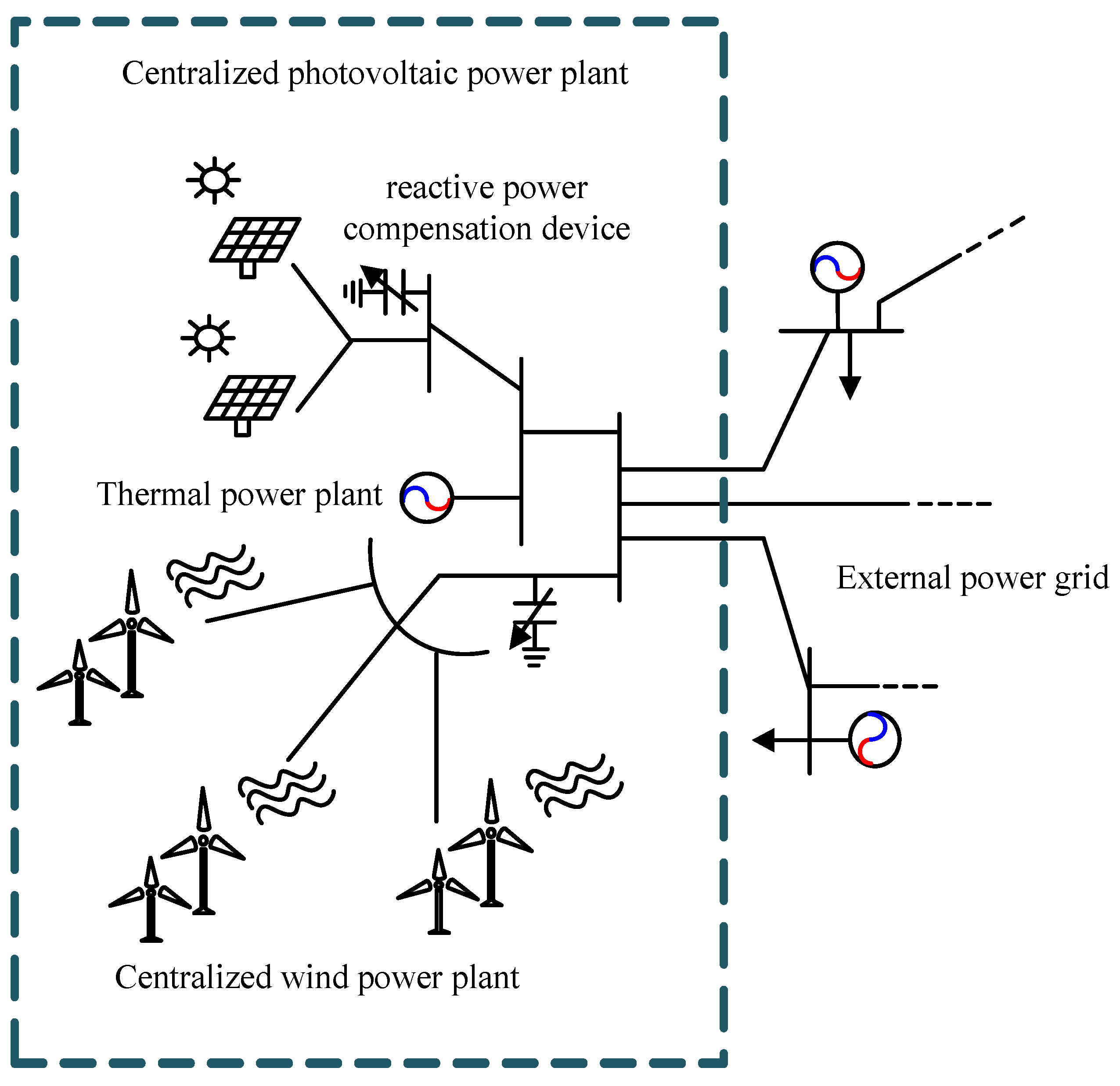
2.1. Spatial Distribution Characteristics of the Coupled System

A multi-power system consisting of a centralized new energy station such as wind and solar, which has a similar electrical distance in the same area, coupled with traditional thermal power plants through the same junction point is defined as a coupled system, usually as a unified electricity production entity participating in power grid regulation. A schematic diagram is shown in Figure 1. The coupled system has hierarchical characteristics from new energy power units to new energy stations and then to the upper transmission system. The new energy units, new energy stations, and external PCC of the coupled system in this system all need to meet different grid voltage safety standards, which increases the difficulty of internal voltage control in the coupled system. In addition, in the distribution of reactive power control resources in coupled system voltage control, the transmission network mainly relies on traditional synchronous generator units as reactive power sources, and centralized new energy stations usually have continuous reactive power compensation devices such as static var generators (SVGs) installed at PCCs. At the same time, each new energy unit also has a specific reactive power capacity, which can be used for internal reactive power optimization and regulation in the station.

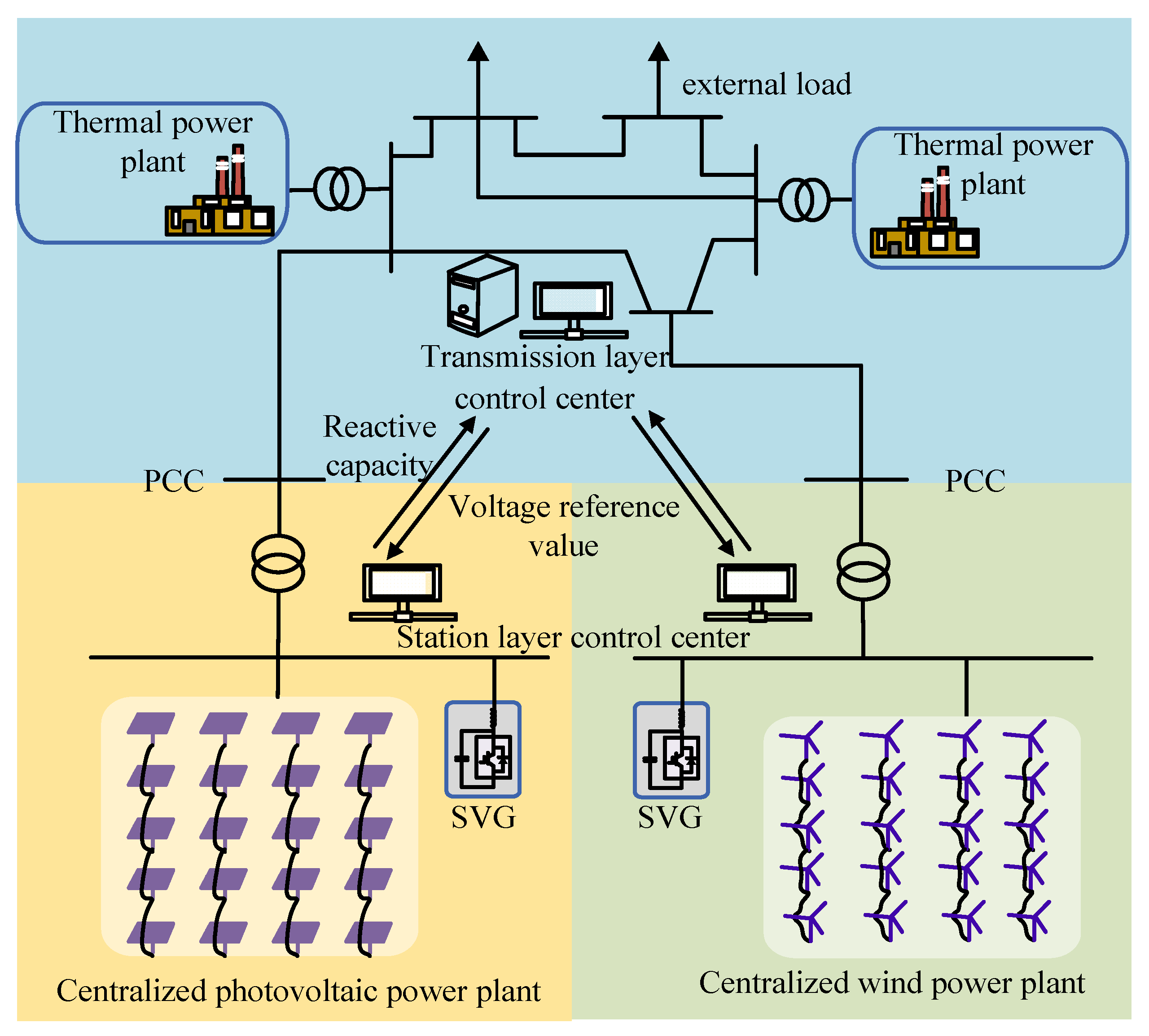
2.2. Collaborative Optimization Control Structure of the Coupled System

The internal transmission network of the coupled system and the centralized new energy station belong to different management systems, which have independent voltage requirements and operating standards. Due to data privacy protection and other reasons, various systems can read and use the boundary node information of substations located only at the junction of the transmission network and centralized new energy power stations. As shown in Figure 2, for the reactive power and voltage collaborative optimization problem of the coupled system, the coupled system is decomposed into the transmission layer and station layer to reduce optimization complexity. Different layers have autonomous capabilities, and only limited communication transmission is required. The entire system can be optimized by using the controller at this layer to call reactive power resources in the local area. Among them, the transmission layer is regarded as the upper central system, which includes thermal power plants, transmission network, and new energy stations, At this time, disregarding the internal voltage fluctuations of the new energy station, the entire station is regarded as a power source that transmits power to the outside through the PCC. The transmission layer controller utilizes the output of the thermal power units and the reactive power output of the power station to regulate the reactive voltage of critical nodes in the transmission layer and sends the regulated voltage at the PCC of the power station as a reference command to each station controller. Each centralized new energy station serves as a lower-layer subsystem when each station controller receives the voltage reference command issued by the PCC. In order to maximize the utilization of the reactive power regulation capacity of the power units, the initial reactive power voltage demand of the station is first calculated to determine the activation status of reactive power control resources within the station. Then, voltage control is carried out on the station layer based on the received voltage command. Finally, the station transfers the remaining adjustable reactive power to the transmission layer for the following regulation moment.

Therefore, this article takes the voltage at the PCC between the transmission network and each station as a coupling variable and only boundary voltage information needs to be transmitted between different systems to adjacent systems, satisfying the following consistency constraints:

$$U_{PCC,i}^S-U_{PCC,i}^C=0, i\in \left[1,\dots ,\alpha \right]$$

(1)

where $U_{PCC,i}^S$ represents the voltage at the PCC between the transmission network layer and the i-th new energy station, and α indicates the number of new energy stations.

3. Collaborative Reactive Power Optimization Control of the Coupled System

3.1. Predictive Model Based on Sensitivity Theory

In actual operating systems, due to the real-time fluctuation of the load and power of new energy stations, an intelligent algorithm is used to solve the distributed reactive power optimization of the coupled system, which not only increases computational complexity but also causes problems such as getting stuck in local optima. Reference [25] points out that sensitivity is a physical quantity that reflects the sensitivity of a system’s state or output changes to minor changes in system parameters. Therefore, the sensitivity of control objectives and control variables is obtained to finely and quickly adjust various control resources based on the AC power flow equation. The nonlinear power flow equation is linearized at the steady-state solution, and the voltage prediction model is obtained as follows:

$$U_n=U_n^0+{\displaystyle \sum _{\mathrm{j}=1}^{{\mathrm{N}}_{\mathsf{\mu }}}\frac{\mathsf{\Delta }{\mathrm{U}}_{\mathrm{n}}}{\mathsf{\Delta }{\mathsf{\mu }}_{\mathrm{j}}}\mathsf{\Delta }{\mathsf{\mu }}_{\mathrm{j}}}$$

(2)

where $U_n^0$ is the initial steady-state voltage of node n, $N_{\mu }$ is the number of control variables, $\mathsf{\Delta }{\mu }_j$ is the control variable involved in regulation within the region, and $\mathsf{\Delta }{U}_n/\mathsf{\Delta }{\mu }_j$ is the sensitivity matrix of the voltage vector of node n to the j-th control resource variable, obtained through the perturbation method, representing the ability of each control variable to affect node voltage.

Meanwhile, based on references [4,26], the following objective functions and related constraints at different layers are established.

3.2. Optimization Model of the Transmission Layer

3.2.1. Transmission Layer Objective Function

The transmission layer sends the output power of thermal power and new energy to the outside through ultra-high voltage and long-distance transmission channels; it will impact the voltage of its internal PCC. Therefore, to ensure that the voltage at the high-voltage PCC of the transmission layer and the PCC of the new energy station are not affected by external load fluctuations and other factors, these nodes are selected as key nodes in the transmission layer. The minimum sum of squared deviations between key nodes and voltage reference values is set as the objective function of the transmission layer, expressed as:

$$\min f_U^S(\mathsf{\Delta }{\mu }_t^S)={\displaystyle \sum _n{(U_{n,t}^S-U_{ref}^S)}^2}$$

(3)

where n is the key node of the transmission layer; $U_{n,t}^S$ is the voltage prediction information vector at time t for each key node in the transmission layer, obtained from Equation (2); $U_{ref}^S$ is the reference voltage vector for the voltage at the PCC of the transmission layer; $\mathsf{\Delta }{\mu }_t^S$ is the vector of changes in various control resources at time t of the transmission layer, $\mathsf{\Delta }{\mu }_t^S=[\mathsf{\Delta }{U}_{g,t}^S,\mathsf{\Delta }{P}_{g,t}^S,\mathsf{\Delta }{Q}_{sta,t}^S]$; $\mathsf{\Delta }{U}_{g,t}^S$ is the adjustment amount of the terminal voltage of the thermal power plant at time t; $\mathsf{\Delta }{P}_{g,t}^S$ is the adjustment amount of active output of the thermal power plant at time t; and $\mathsf{\Delta }{Q}_{sta,t}^S$ is the overall available reactive power adjustment of each new energy station at time t.

3.2.2. Constraints of the Transmission Layer

(1)

Node voltage safety constraints:

$$U_{i\min }\le U_{n,t}^S\le U_{i\max }$$

(4)

where $U_{i\min }$ and $U_{i\max }$ are the lower and upper limits of the node voltage amplitude. The voltage standards at different layers have different values.

(2)

Power output constraints of thermal power plants:

$$P_{g\min }\le P_{g,t}^S\le P_{g\max }$$

(5)

where $P_{g,t}^S$ is the active output of the thermal power plant at time t, and $P_{g\max }$ and $P_{g\min }$ are the upper and lower limits of their active output.

(3)

Station transmission reactive power constraint:

$$Q_{sta}^{S,\min }\le Q_{sta,t}^S\le Q_{sta}^{S,\max }$$

(6)

where $Q_{sta,t}^S$ is the total reactive power regulation amount transmitted by each station to the outside at time t of the transmission layer, and $Q_{sta}^{S,\max }$ and $Q_{sta}^{S,\min }$ are the upper and lower limits of the available reactive power compensation at the station.

3.3. Optimization Model for the Station Layer

3.3.1. Initial Reactive Power Demand Allocation at the Station Layer

The types of centralized new energy stations are mainly divided into wind power plants and photovoltaic power plants. The control resources at this layer are the adjustable reactive power capacity of the internal power unit of each station and continuous reactive power compensation devices. For a new energy station containing N power units, the total reactive power limit that the power units can output at time t is:

$$\left\{\begin{array}{l}{Q}_{C\max }={\displaystyle \sum _{i=1}^N{Q}_{Ci\max }}\\ Q_{C\min }={\displaystyle \sum _{i=1}^N{Q}_{Ci\min }}\end{array}\right.$$

(7)

where N is the total number of power units in the station, and $Q_{Ci\max }$ and $Q_{Ci\min }$ are the upper and lower limits of reactive power output for a single unit, represented as:

$$Q_{Ci\max }=\sqrt{S_{Ci}^2-P_{Ci}^2}$$

(8)

$$Q_{Ci\min }=-\sqrt{S_{Ci}^2-P_{Ci}^2}$$

(9)

$S_{Ci}$ is the rated apparent power of the power unit, and $P_{Ci}$ is the active output of the power unit.

Because continuous reactive power compensation devices can quickly respond to the reactive power demand of the power grid, during system disturbances and faults, they can promptly compensate or absorb the system’s reactive power. Therefore, when coordinating the continuous compensation device at the station layer with the power unit’s reactive power output, prioritize adjusting each unit’s reactive power output so it can reserve more dynamic reactive power compensation capacity for the system. Considering that while new energy stations transmit power to external transmission lines, the internal unit is easily affected by the environment, and the output has randomness and fluctuation. To ensure the voltage safety of the PCC and internal units, the station’s initial reactive power demand can be determined by issuing instructions from the transmission layer and internal active power changes within the station.

After conducting reactive voltage control on the transmission layer, based on meeting the voltage control requirements of this layer, distribute the required reactive power output and grid voltage reference values to each station controller. At time t, each station controller receives instructions, according to Equation (10), to calculate the reactive power demand that meets the voltage requirements of the PCC of the upper transmission system:

$$\mathsf{\Delta }{Q}_1=Q_S+Q_{Closs}$$

(10)

where $Q_S$ is the reactive power the entire station needs to transmit to the transmission layer; $Q_{Closs}$ is the reactive power loss inside the station during actual reactive power transmission.

On this basis, consider the impact of active power output fluctuations at adjacent times of new energy stations on the terminal voltage of each unit, assuming that during the reactive voltage control cycle at the station layer, the voltage deviation caused by the change in active output of adjacent units within the station for a single unit is $\mathsf{\Delta }{U}_{G_{i-o}}$:

$$\mathsf{\Delta }{U}_{G_{i-o}}={\displaystyle \sum _{i=1}^m{\displaystyle \sum _{j=1}^n\left(\frac{\mathsf{\Delta }{U}_{G_{i-o}}}{\mathsf{\Delta }{P}_{G_{i-j}}}\mathsf{\Delta }{P}_{G_{i-j}}\right)}}$$

(11)

where m and n, respectively, represent the number of collecting lines and the number of power units on the collecting lines. $\mathsf{\Delta }{U}_{G_{i-o}}$ is the change in terminal voltage of the o-th unit on the i-th collection line, $\mathsf{\Delta }{P}_{G_{i-j}}$ is the active power change in the j-th unit on the i-th collection line at adjacent times, and $\mathsf{\Delta }{U}_{G_{i-o}}/\mathsf{\Delta }{P}_{G_{i-j}}$ is the sensitivity coefficient of the unit terminal voltage to the active output of each unit.

The station layer controller can follow Equations (12) and (13) and calculate the change in terminal voltage caused by changes in active output for all units inside the station. Thus, calculate the magnitude of the reactive power change corresponding to each unit to offset this voltage change:

$$\begin{array}{l}\mathsf{\Delta }{U}_{G_{i-o}}={\displaystyle \sum _{i=1}^m{\displaystyle \sum _{j=1}^n\left(\frac{\mathsf{\Delta }{U}_{G_{i-o}}}{\mathsf{\Delta }{P}_{G_{i-j}}}\mathsf{\Delta }{P}_{G_{i-j}}\right)}}\\ =-{\displaystyle \sum _{i=1}^m{\displaystyle \sum _{j=1}^n\left(\frac{\mathsf{\Delta }{U}_{G_{i-o}}}{\mathsf{\Delta }{Q}_{G_{i-j}}}\mathsf{\Delta }{Q}_{G_{i-j}}\right)}}\end{array}$$

(12)

$$\left[\begin{array}{c}\mathsf{\Delta }{Q}_{G1-1}\\ ⋮\\ \mathsf{\Delta }{Q}_{Gm-n}\end{array}\right]=-{\left[\begin{array}{ccc}\frac{\mathsf{\Delta }{U}_{G1-1}}{\mathsf{\Delta }{Q}_{G1-1}}& \cdots & \frac{\mathsf{\Delta }{U}_{G1-1}}{\mathsf{\Delta }{Q}_{Gm-n}}\\ ⋮& & ⋮\\ \frac{\mathsf{\Delta }{U}_{Gm-1}}{\mathsf{\Delta }{Q}_{G1-1}}& \cdots & \frac{\mathsf{\Delta }{U}_{Gm-n}}{\mathsf{\Delta }{Q}_{Gm-n}}\end{array}\right]}^{-1}\left[\begin{array}{c}\mathsf{\Delta }{U}_{G1-1}\\ ⋮\\ \mathsf{\Delta }{U}_{Gm-n}\end{array}\right]$$

(13)

where $\mathsf{\Delta }{Q}_{G_{i-j}}$ is the reactive power variation in the j-th unit on the i-th collection line. $\mathsf{\Delta }{U}_{G_{i-o}}/\mathsf{\Delta }{Q}_{G_{i-j}}$ is the sensitivity coefficient of the unit terminal voltage to the reactive power output of each unit. Furthermore, Equation (14) can be used to calculate the total reactive power $\mathsf{\Delta }{Q}_2$ required by all units within the station to offset voltage fluctuations caused by active power changes:

$$\mathsf{\Delta }{Q}_2={\displaystyle \sum _{i=1}^m{\displaystyle \sum _{j=1}^n\mathsf{\Delta }{Q}_{Gi-j}}}$$

(14)

Finally, the total initial reactive power demand at the station layer $Q_{ref}$, according to Equation (15), can be calculated as:

$$Q_{ref}=\mathsf{\Delta }{Q}_1+\mathsf{\Delta }{Q}_2$$

(15)

After receiving instructions from the transmission layer, the station layer controller first distributes the reactive power output $\mathsf{\Delta }{Q}_1$ of the station that meets the voltage requirements of the PCC at the transmission layer in proportion to the reactive power capacity of each unit in the station, then calculates and allocate the reactive power demand that meets the active power fluctuations of the unit according to Equations (11)–(15). The total reactive power demand $Q_{ref}$ of the on-site station is higher than its total reactive power limit, or when some units within the station have reached their reactive power limit after initial allocation, the power units within the station that have reached the reactive power limit are at total capacity. Units that have not reached the reactive power limit shall be allocated reactive power according to the result obtained in Equation (13) and activate the continuous reactive power compensation device inside the station so that the continuous reactive power compensation device and the station power unit can jointly participate in the next step of reactive power optimization. Otherwise, allocate reactive power to the power units according to Equation (13) and do not invest in continuous reactive power compensation devices within the station.

3.3.2. Station Layer Objective Function

The terminal voltage of each unit in a centralized new energy station is affected by frequent fluctuations in active power output and spatial distribution differences within the station. To improve the stability of station operation and reduce the impact of internal voltage fluctuations on the power grid, the station’s reactive voltage optimization calculation is carried out after the initial reactive power allocation. The objective function of the adjustment is to minimize the sum of squares of the deviations between the voltage values of the power units and the PCC, respectively, and the reference voltage value at the station layer:

$$\min f_U^C(\mathsf{\Delta }{\mu }_t^C)={(U_{n,t}^C-U_{ref}^C)}^2+{\displaystyle \sum _i^N{(U_{i,t}^C-U_{ref}^C)}^2}$$

(16)

where $U_{n,t}^C$ is the voltage state information vector of PCC at time t of the station layer, and $U_{ref}^C$ is the voltage state information vector at time t inside the new energy station, and it takes the reference voltage value of PCC issued by the transmission system. $\mathsf{\Delta }{\mu }_t^C$ is the station control resource vector at time t of the station layer, $\mathsf{\Delta }{\mu }_t^C=[\mathsf{\Delta }{Q}_{i,t}^C,\mathsf{\Delta }{Q}_{G,t}^C]$; $\mathsf{\Delta }{Q}_{i,t}^C$ is the reactive power compensation adjustment amount of the i-th unit in the station at time t and $\mathsf{\Delta }{Q}_{G,t}^C$ is the adjustment amount of reactive power compensation for the continuous reactive power compensation device in the station at time t.

3.3.3. Station Layer Constraints

In addition to meeting the voltage safety constraints of Equation (4), at time t, each power unit and the continuous reactive power compensation device installed on the low-voltage side of the PCC at the site station also need to meet the following constraints:

$$Q_{Ci\min }-Q_{i-L,t}\le Q_{i,t}^C\le Q_{Ci\max }-Q_{i-C,t}$$

(17)

$$Q_{G,\min }^C\le Q_{G,t}^C\le Q_{G,\max }^C$$

(18)

where $Q_{i,t}^C$ is the reactive power output of each unit in the station at time t, $Q_{i-L,t}$ and $Q_{i-C,t}$ are the initial allocation of inductive and capacitive reactive power capacity for each unit of the station at time t, $Q_{G,t}^C$ is the reactive power output of the continuous reactive power compensation device in the station at time t, and $Q_{G,\max }^C$ and $Q_{G,\min }^C$ are the upper and lower limits of the output of continuous reactive power compensation devices in each new energy field station.

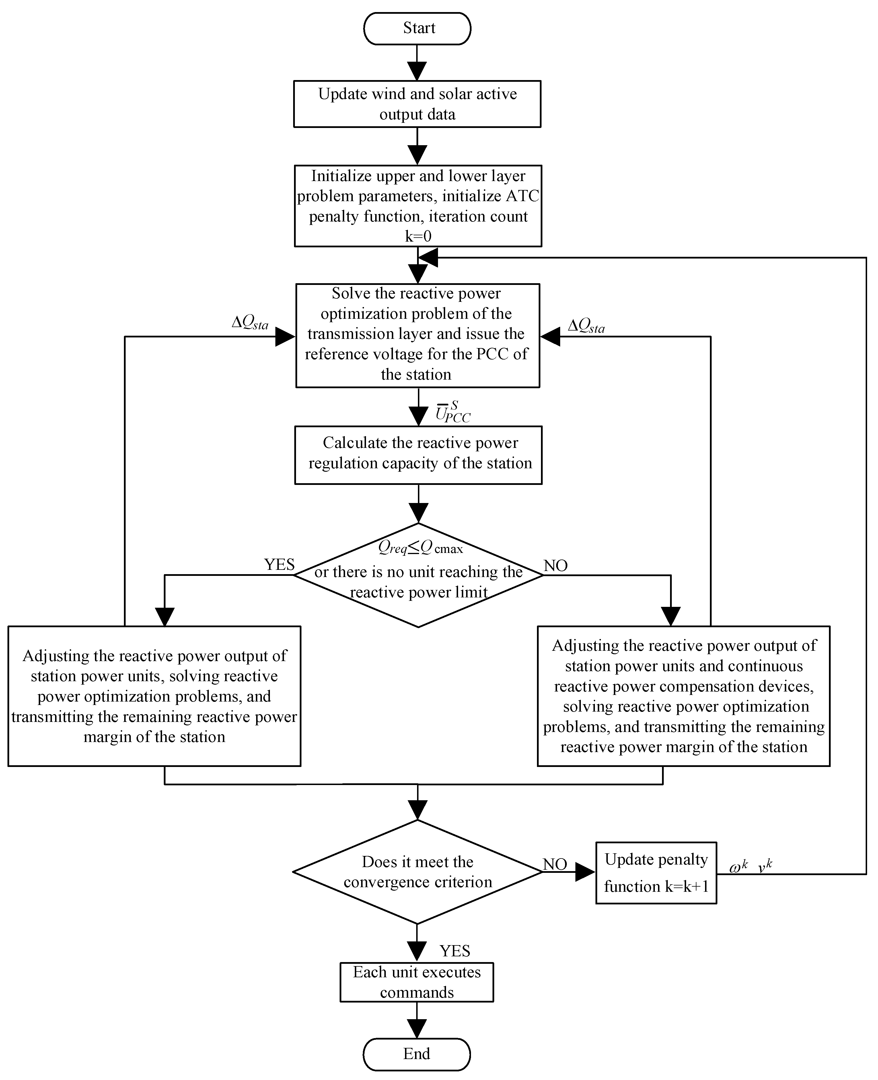
4. Collaborative Reactive Power Optimization Method for the Coupled System

The basic idea of analytical target cascading is to design optimization objectives at the system and subsystem layers. It allows each optimization subject in the hierarchical structure to make autonomous decisions, and the objective function is allocated from top to bottom; simultaneously responding to continuous feedback from bottom to top, the system layer and subsystem layer problems are independently optimized, iterating alternately until convergence is achieved [27]. In using the ATC theory for distributed solving, each layer of the subject can set its optimization model. The variables commonly contained in the optimization model of each layer and among other layers are collaborative.

The distributed collaborative optimization problem of the coupled system is a multi-layer, multi-agent, and multi-step complex nonlinear mixed integer programming problem in mathematics. To achieve decentralized autonomy and collaborative optimization in various regions, based on Equation (1) consistency constraints, the consistency constraints are relaxed in the form of augmented Lagrangian penalty functions to the control objective functions of the transmission layer and station layer through the ATC principle and decomposed into a collaborative control problem between the transmission layer and the station layer for an iterative solution, thereby achieving complete decoupling of the regional problem.

In summary, modify the objective function of the transmission layer as shown in Equation (19):

$$\left\{\begin{array}{l}{J}^S=\min \left\{\begin{array}{l}{f}_U^S(\mathsf{\Delta }{\mu }_t^S)\\ +{\displaystyle \sum _{i=1}^{\alpha }\begin{array}{l}{v}_i^t\left(U_{PCC,t,i}^S-{\overline{U}}_{PCC,t,i}^C\right)\\ +{\omega }_i^t{\left(U_{PCC,t,i}^S-{\overline{U}}_{PCC,t,i}^C\right)}^2\end{array}}\end{array}\right\}\\ Equations \left(4\right)-\left(6\right)\end{array}\right.$$

(19)

where $f_U^S(\mathsf{\Delta }{\mu }_t^S)$ is the optimization function for reactive power and voltage in the transmission layer, ${\overline{U}}_{PCC,t,i}^C$ is the solution value of the coupling variable transmitted from the i-th station layer to the transmission layer at time t, and $v_i^t$ and ${\omega }_i^t$ are the multipliers of the primary and quadratic terms of the penalty function for the i-th new energy station at time t.

The objective function of the station layer is modified to Equation (20) as follows:

$$\left\{\begin{array}{l}{J}^C=\min \left\{\begin{array}{l}{f}_U^C(\mathsf{\Delta }{\mu }_t^C)\\ +v^t\left(U_{PCC,t}^C-{\overline{U}}_{PCC,t}^S\right)\\ +{\omega }^t{\left(U_{PCC,t}^C-{\overline{U}}_{PCC,t}^S\right)}^2\end{array}\right\}\\ Equations \left(17\right) and \left(18\right)\end{array}\right.$$

(20)

where $f_U^C(\mathsf{\Delta }{\mu }_t^C)$ is the reactive voltage optimization function for centralized new energy stations, and ${\overline{U}}_{PCC,t}^S$ is the solution value of the coupling variable transmitted from the transmission layer to the station layer at time t.

The ATC method essentially belongs to the multiplier method in optimization methods. Reference [28] has obtained strict theoretical proof of its convergence. The convergence conditions of the distributed reactive power optimization algorithm for the coupled system based on the ATC principle in this article are:

$$‖U^{S,k}-U^{C,k}‖\le {\epsilon }_1$$

(21)

$$\max \left[‖U^{S,k+1}-U^{S,k}‖,‖U^{C,k+1}-U^{C,k}‖\right]\le {\epsilon }_2$$

(22)

where Equation (21) represents the coupling variable of the grid voltage between the transmission layer and the station layer in the k-th iteration. The difference should meet the convergence accuracy ${\epsilon }_1$. Equation (22) represents whether the difference between the coupling variables of the decomposed transmission layer and the station layer at their respective layers in adjacent iterations is optimal and should meet the convergence accuracy ${\epsilon }_2$. If the convergence criteria Equations (21) and (22) cannot be satisfied simultaneously, then update the penalty function’s first and second multipliers according to Equations (23) and (24):

$$v^{k+1}=v^k+2{({\omega }^k)}^2(U_{PCC}^{S,k}-U_{PCC}^{C,k})$$

(23)

$${\omega }^{k+1}=\beta {\omega }^k$$

(24)

where $v^k$ and ${\omega }^k$ represent the multipliers of the primary and quadratic terms of the penalty function in the k-th iteration. β is expressed as the penalty parameter amplification factor, the general range of values to ensure convergence is 2–3, and $U_{PCC}^{S,k}$ and $U_{PCC}^{C,k}$, respectively, represent the consistency variables obtained in the k-th iteration for the upper and lower layer problems, namely the voltage at the PCC of the new energy station.

Overall, the flowchart of distributed reactive power optimization control based on the ATC coupled system is shown in Figure 3:

5. Results and Discussion

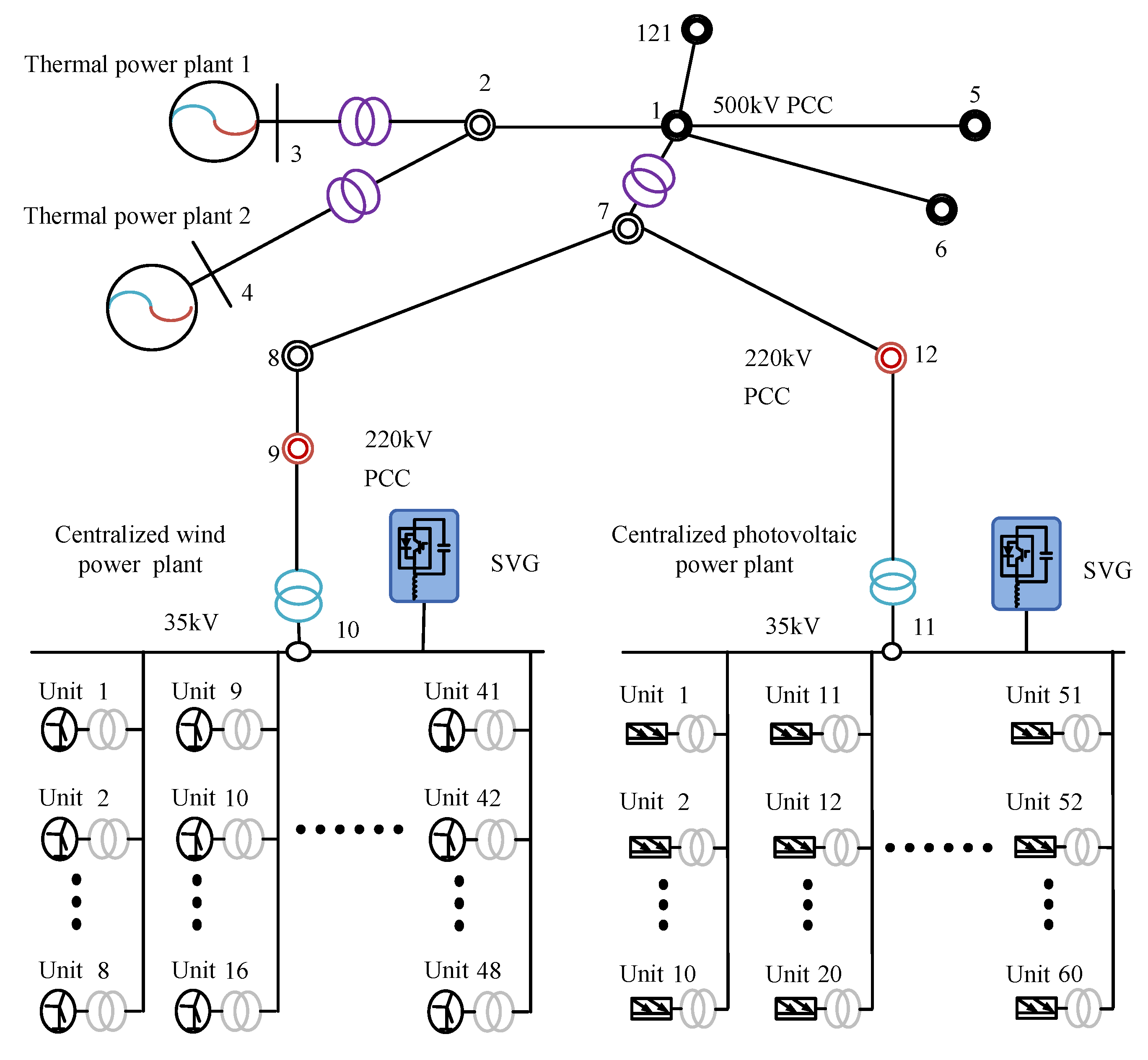
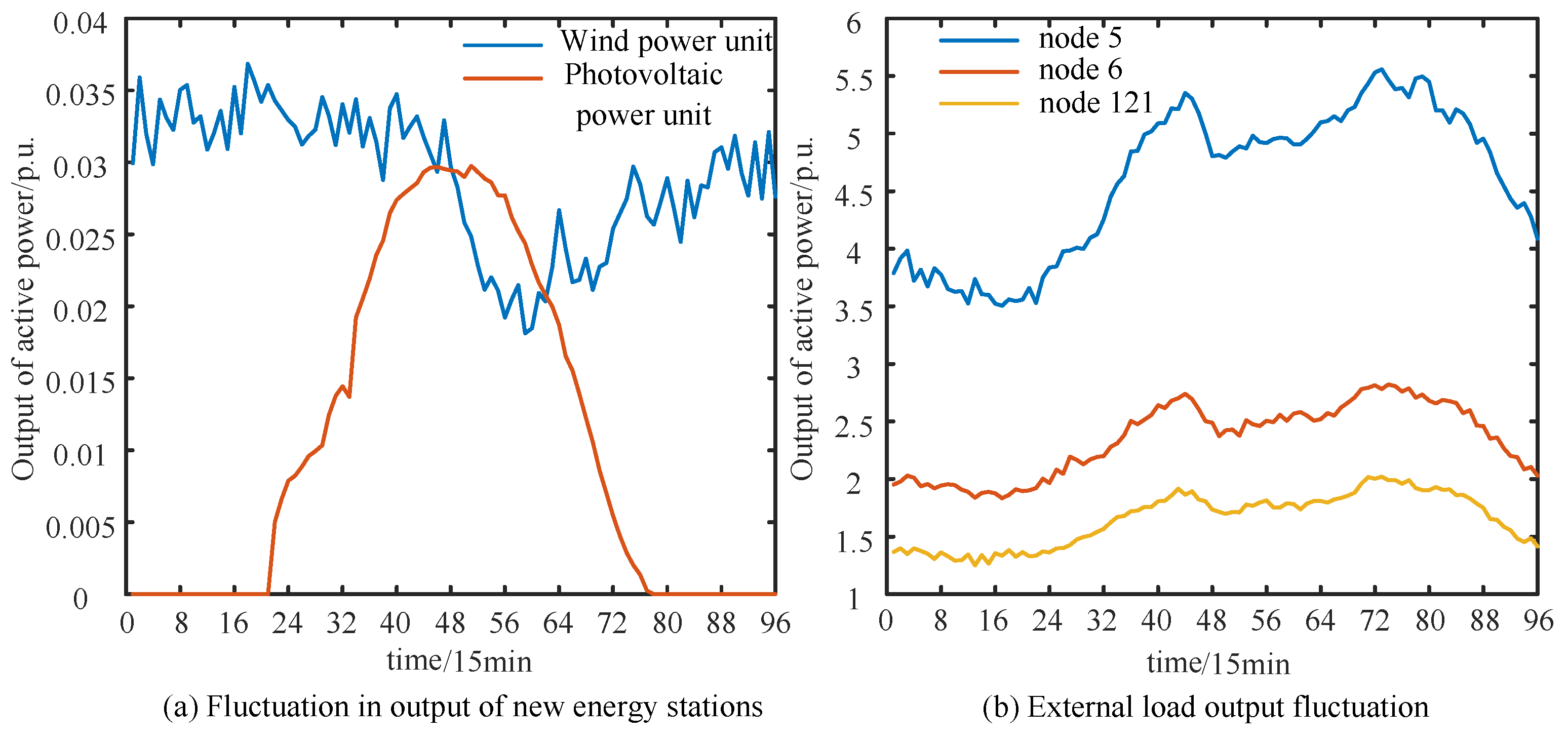
5.1. Example Description

This article takes the coupled system composed of the centralized new energy station and the traditional thermal power plant in a certain region of Dalian as an example to verify the feasibility of the proposed distributed collaborative control strategy. The power grid structure is shown in Figure 4. The regional power grid has two 20 kV thermal power plants, busbar 3 located in thermal power plant 1 is selected as the balance node within the system, the rated installed capacity of thermal power plant 2 is set to 400 MW, and the initial voltage of the two thermal power plants is set to 1.0 p.u. The total installed capacity of the wind power plant is 192 MW, including 48 wind turbines with a rated terminal voltage of 0.7 kV. The total installed capacity of the photovoltaic power plant is 210 MW, including 60 photovoltaic turbines with a rated terminal voltage of 0.4 kV. A continuous reactive power compensation device (SVG) with a capacity range of [−30, 30] Mvar is installed on the low-voltage side of the PCC within the wind and solar power plant. Node 1 is the 500 kV PCC of the coupled system; nodes 9 and 12 are the PCCs between the wind and solar power plant and the external transmission system, respectively. Their voltages are taken as the consistency constraint variables. The output prediction curve of the station unit refers to Figure 5a. It can be observed that the active power output of wind power fluctuates greatly throughout the day, with higher output at night and in the morning. At the same time, the active power output of photovoltaic power generation increases with the increase in light intensity during the day and is higher in the noon range. Nodes 5, 6, and 121 represent the external transmission nodes of the system, and their active power changes represent the active power demand of the load on the external transmission line during the day. The predicted value curve is shown in Figure 5b. The voltage safety range at the PCC and power units in the centralized new energy station is set to [0.97, 1.07] p.u., according to technical standards. The voltage safety range of the 500 kV PCC in the transmission layer system is set to [0.99, 1.01] p.u., and the interval between each control moment is 15 min.

The benchmark capacity of the entire system is set to 100 MVA. To reduce algorithm complexity, it is assumed that the model parameters of each unit in the centralized wind and solar power plant are consistent and have the same power output capacity. The penalty function of the ATC algorithm primary term and quadratic term multiplier $v_i^t$ and ${\omega }_i^t$, both with initial values of 0.0725, β takes 2.15, and the convergence accuracy ${\epsilon }_1$, ${\epsilon }_2$ is taken as 0.005 and 0.006, respectively. The simulation platform used in this article is the AMD Ryzen 7 5800H @3.20 GHz model with Windows 11 Home Edition, and the simulation modeling software used was MATLAB 2019b.

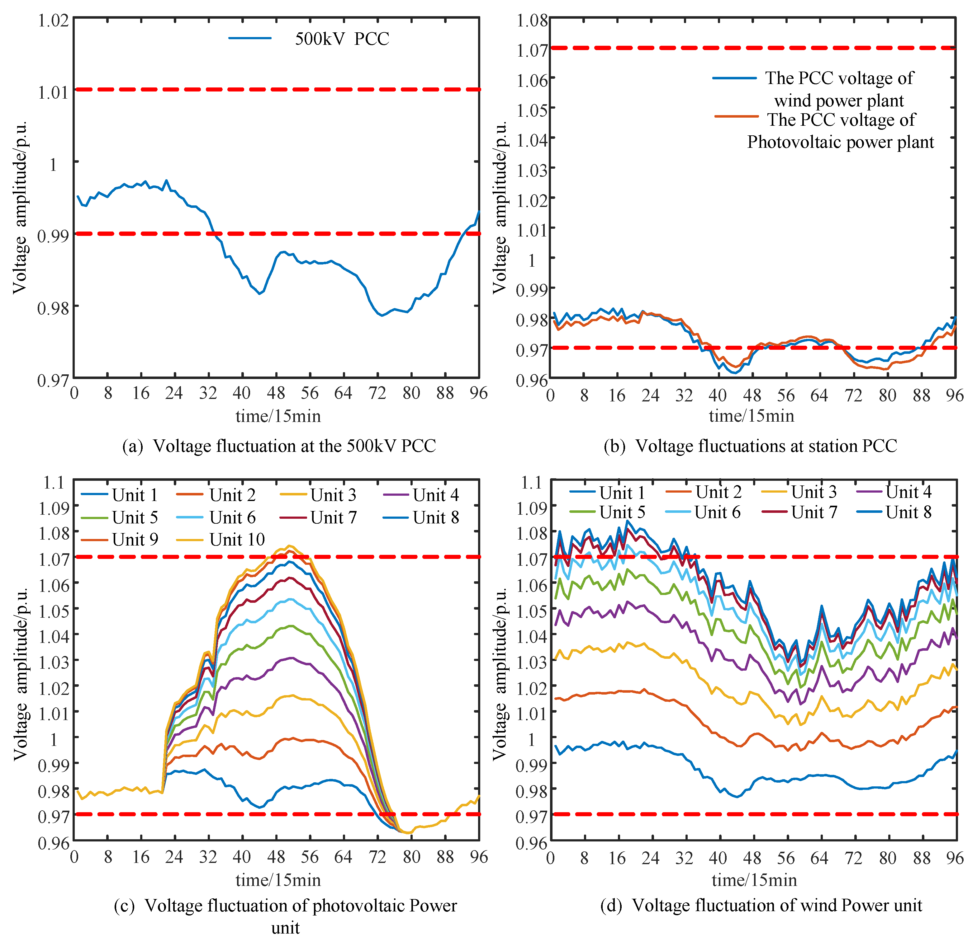
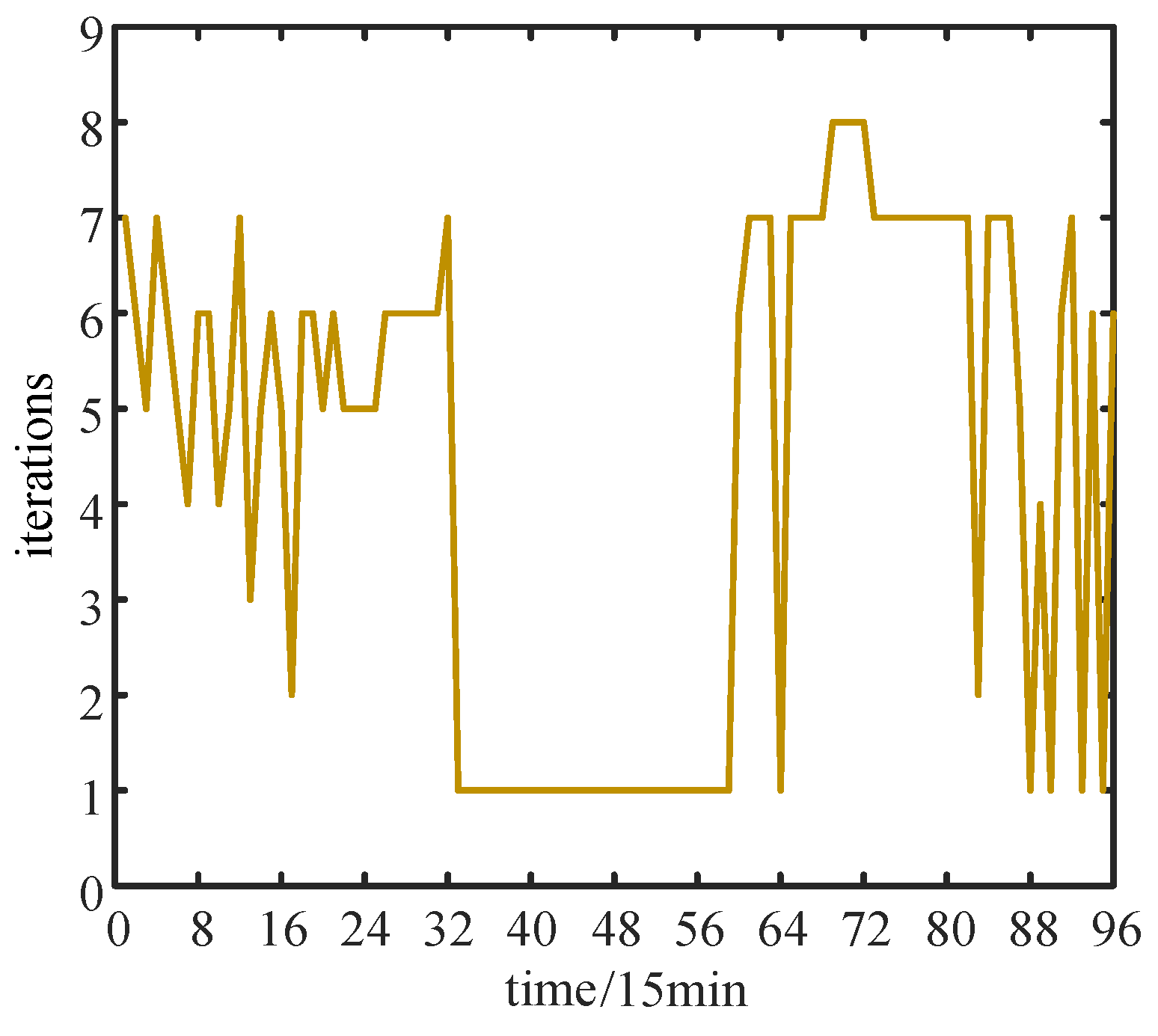
5.2. Performance Analysis of Distributed Reactive Power Optimization

Figure 6 shows the voltage status of each PCC and unit terminal of the coupled system transmission layer and station layer within 24 h a day before regulation. As shown in Figure 6a,b, the transmission layer gathers the overall output of wind, solar, and thermal power to transmit power externally. The 500 kV PCC is not only affected by the output of internal units but also by external load fluctuations, causing its voltage to operate within a safe range during low load periods, while during peak load periods, it is lower than the engineering regulations by 0.99 p.u. The voltage changes at the PCC of the new energy station are similar to that at the 500 kV PCC. However, because most of the time, the PCCs of the plants send out relatively large active power, and each new energy station is located at the end of the transmission network, the impact of load fluctuations on them is relatively small, resulting in a lighter degree of voltage exceeding the limit. The maximum voltage deviation of the 500 kV PCC and the PCC of the wind and solar power plant throughout the day are 0.0188 p.u., 0.0214 p.u., and 0.0191 p.u., respectively. Figure 6c,d show the changes in the terminal voltage of the internal power units of the wind and solar power plant before regulation, and the analysis is conducted on a single collecting line within the plant. It can be observed that each unit of a power transmission line is affected by the parameters of the transmission line within the station and the spatial distribution of the units. The closer the distribution of units is to the PCC, the more similar the fluctuation trend of the plant terminal voltage is to the PCC throughout the day. At the same time, under the same output conditions of the unit, like the distance from the unit to the PCC, the terminal voltage of the unit increases in sequence, and the terminal voltage of the unit at the end of the plant may exceed the limit to varying degrees at times of high wind and solar output, which has adverse effects on the safe and stable operation of each plant. The maximum deviation of the terminal voltage of the wind and solar power plant at the same time throughout the day is 0.0886 p.u. and 0.0946 p.u., respectively.

The results of optimizing the control strategy in this article are shown in Figure 7. It can be seen that this method effectively controls the voltage at the PCC of the new energy station and the voltage at the 500 kV PCC within their respective specified voltage safety ranges. The maximum voltage differences are 0.0021 p.u., 0.0057 p.u., and 0.0056 p.u., which to some extent reduces the voltage fluctuations at each PCC and ensures a more stable voltage compared to before regulation while ensuring that the voltage does not exceed the limit. The terminal voltage of power units of wind and solar power plants distributed in different spatial positions can be effectively controlled within the safe voltage range throughout the day. At the same time throughout the day, the maximum deviation of the terminal voltage of the first and last units is reduced to 0.0847 p.u. and 0.0929 p.u. This indicates that the strategy proposed in this article can effectively meet the voltage requirements between different regions within the coupled system.

On the premise that the voltage in each area can be maintained within a safe range, the corresponding cumulative network loss results for the whole day are shown in

Table 1. Accumulated network loss results for the entire day.

Title 1	Before Regulation (p.u.)	After Regulation (p.u.)
Transmission layer	28.6719	28.5004
Wind power plant	9.0037	9.9893
Photovoltaic power plant	3.8966	4.0388

. Due to the significant impact of external loads on the transmission layer, the voltage is mostly below the lower limit. After regulation, the overall voltage level is closer to the rated voltage, resulting in a decrease in the cumulative network loss of the transmission layer compared to before regulation. However, due to the influence of geographical location and external environmental factors, the voltage level of power units in each station is often close to its limit, and there is very little room for optimization. This leads to increased cumulative network losses throughout the day compared to before regulation while meeting voltage constraints. If the network structure is strengthened and improved, the space for reducing losses may be more significant.

Distributed solving is an iterative optimization process, and Figure 8 shows the results of the number of iterations in each period throughout the day during the collaborative control process. In the initial situation, the values of the primary and quadratic term multipliers of the penalty function are small, and the weight of consistency constraints in the objective process is negligible. In most cases, the residual cannot meet the convergence accuracy after one iteration, and setting the penalty parameter amplification factor β plays a role in accelerating the convergence speed. As the number of iterations increases, different layers can independently update the primary and quadratic term, gradually increasing the weight of consistency constraints in the objective function and improving the convergence effect of the residual solution. It can be seen that using the ATC method to solve the reactive power optimization within the system can strictly converge after a maximum of eight iterations throughout the day. In summary, the required number of iterations for solving is small, and the communication burden between adjacent controllers is small. While ensuring the reliability of distributed solving, the quality of the obtained optimization solution is improved.

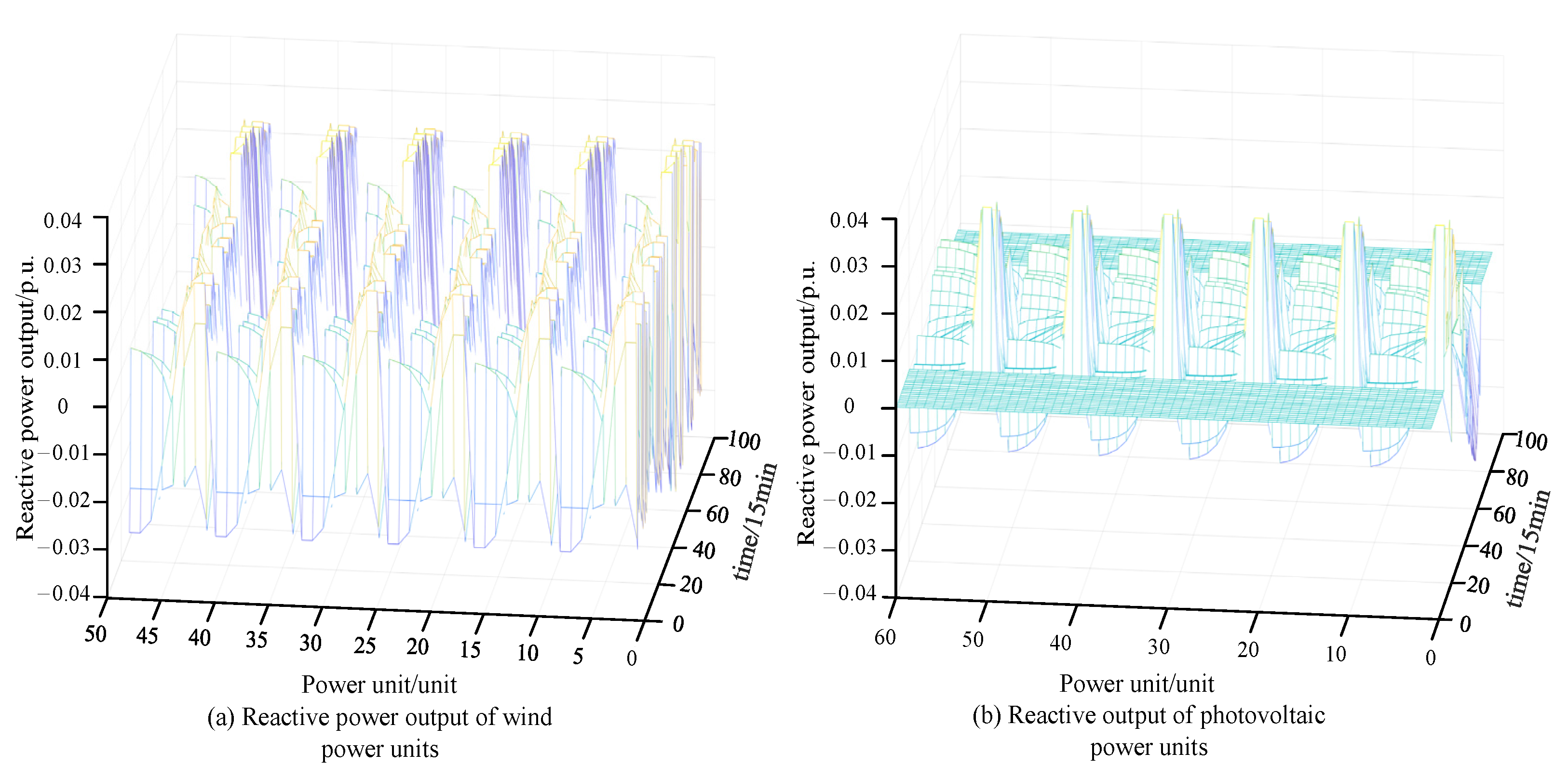
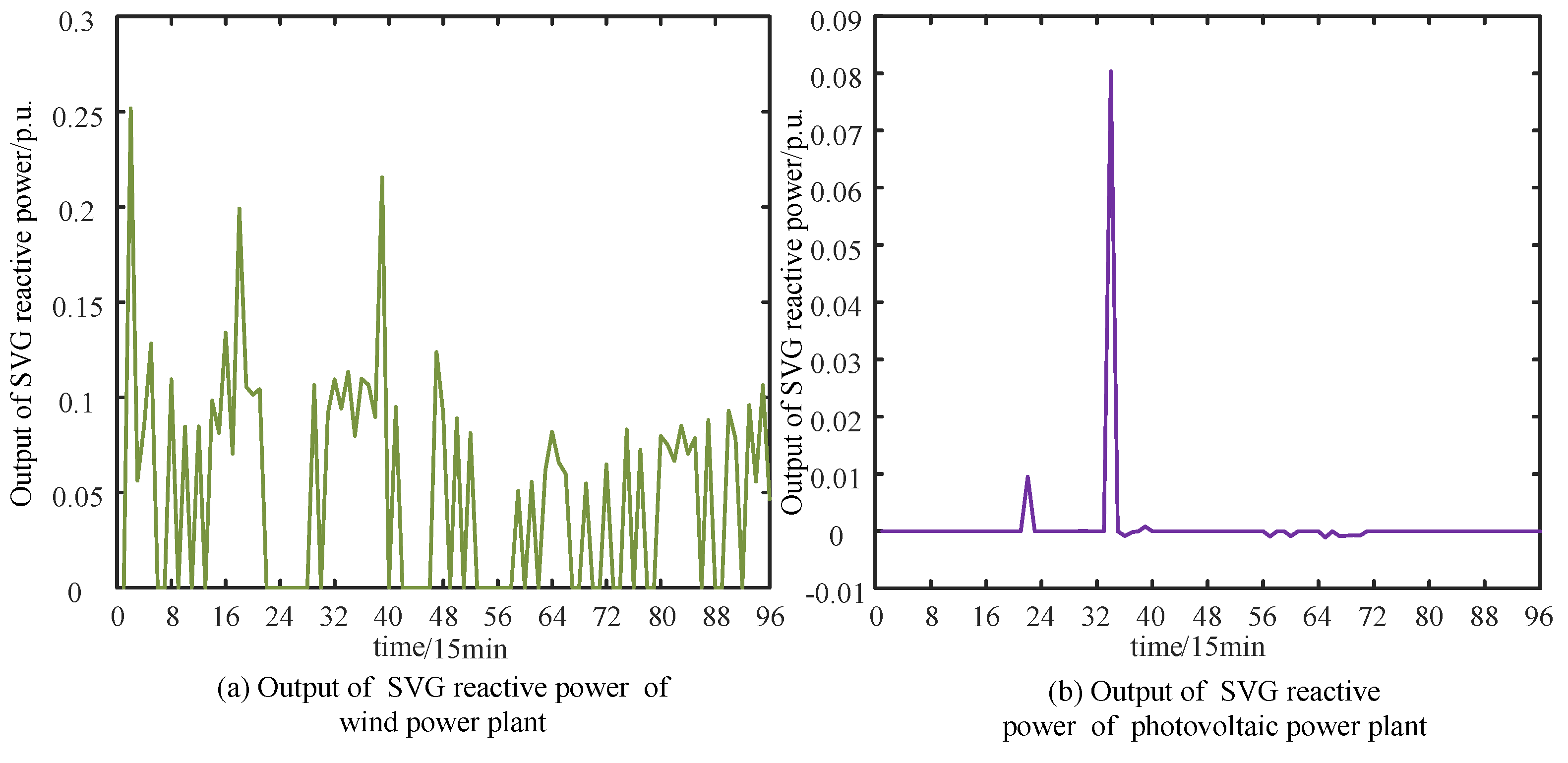
5.3. Analysis of Reactive Power Resource Output in the Coupled System

Figure 9 shows the changes in the control quantity of the transmission layer throughout the day. Two thermal power units are connected to the 500 kV PCC through a 20 kV/500 kV step-up transformer, with a relatively close electrical distance. The wind and solar power plant is located at the end of the transmission network, and the electrical distance from the 500 kV PCC is relatively far. Thermal power units are the main regulating equipment for the transmission layer, and their regulating effect is more pronounced.

As shown in Figure 9a,b, during the reactive power optimization process, the active power of thermal power unit 2 can be controlled, but the amplitude of change is small. The optimization mainly relies on adjusting the terminal voltage of the thermal power unit. The 500 kV PCC of the transmission layer is greatly affected by the load fluctuation of the external transmission channel, causing the terminal voltage of the thermal power unit to be adjusted below the set voltage during the low load period and above the set voltage during the peak load period, consistent with the trend of reverse pressure regulation. Figure 9c shows the variation in reactive power output from new energy power stations. Each station is distributed at the end of the transmission network, and the active power output is greatly affected by the line impedance during the process of being transmitted to the 500 kV high-voltage grid through long lines, increasing active power loss. Therefore, while adjusting the thermal power unit to change the overall voltage level of the transmission layer, The station needs to transmit a certain amount of reactive power to the outside to ensure that the voltage of the PCC and transmission line is maintained within the regulatory standards during active power transmission. Due to the farther distance between the centralized wind power plant PCC and the 500 kV PCC of the transmission layer, the impact of line impedance is more significant, and the reactive power output to the outside is mostly more than that of the centralized photovoltaic power plant.

Figure 10 and Figure 11 show the reactive power changes in the wind and solar power plant unit and the SVG inside the station during reactive power regulation at the station layer. Due to differences in the active power output of new energy sources and the spatial distribution of power units within the station, the degree and magnitude of the reactive power output changes of power units on the same collection line at each time are not the same: for the wind power plant, due to the significant fluctuation of the wind turbine output, the voltage inside the station changes dramatically most of the time, and the demand for reactive power is high. When some power units in the station reach full power, the SVG inside the station needs to be started to meet the control requirements of the station voltage. Moreover, each unit’s frequency range of reactive power output fluctuations is relatively severe, and the regularity is not strong. At the same time, on the same collecting line, power units at different positions will simultaneously emit inductive and capacitive reactive power to improve the impact caused by the spatial position and output fluctuations. The active power output of a photovoltaic power plant is mainly affected by light intensity. In the absence of light, the active power output inside the station is 0, and the voltage fluctuation in the electric field is relatively small. At this time, only the reactive power output of the unit is needed to meet the voltage regulation requirements without the need to use SVG inside the station. When the intensity of light is high, or the amplitude of light changes is large, the active output of photovoltaics rises and falls sharply. At this time, the reactive output of each power unit has a significant increase and decrease. At some times, relying solely on the reactive output of power units makes it difficult to meet the voltage requirements of the station, and SVG needs to be activated. Since light does not change as much as wind speed throughout the day, the number of SVG activations in photovoltaics is less than that in the wind power plant. Figure 11 shows that the strategy proposed in this article can effectively reduce the number of SVG inputs and maximize the reactive power potential of new energy stations compared to the direct input of SVG and the joint regulation of power units.

6. Conclusions

This article focuses on the coupled system composed of new energy power plants and thermal power units, combined with the hierarchical structure characteristics of its internal unit station system, and it adopts hierarchical collaborative control to achieve voltage control from the whole to the local. The following conclusions can be drawn:

(1)

By using the target cascade method for voltage hierarchical collaborative control of the coupled system, the coupled system is divided into multiple sub-optimization control problems based on physical hierarchical characteristics, reducing model size and solving difficulty.

(2)

Adopting different voltage standards for different regions can effectively ensure the safety of voltage operation within the coupled system and reduce network losses to a certain extent.

(3)

Considering the characteristics of reactive power resources within the new energy station, the adjustable reactive power margin of the continuous reactive power compensation device is ensured while fully utilizing the reactive power regulation capacity of the power units of the new energy station.

Finally, the reactive power and voltage collaborative control strategy studied in this article only considers improving the voltage quality of each region, and its objective function is scalable. As long as the objective function meets the requirements of the convex function, it can be solved. Meanwhile, further improving the computational efficiency and accuracy of the model is also one of the issues worth paying attention to.

References

1. Angizeh, F.; Bae, J.; Chen, J.; Klebnikov, A.; Jafari, M.A. Impact Assessment Framework for Grid Integration of Energy Storage Systems and Renewable Energy Sources Toward Clean Energy Transition. IEEE Access 2023, 11, 134995–135005. [Google Scholar] [CrossRef]
2. Yang, L.; Zhou, N.; Zhou, G.; Chi, Y.; Chen, N.; Wang, L.; Wang, Q.; Chang, D. Day-ahead Optimal Dispatch Model for Coupled System Considering Ladder-type Ramping Rate and Flexible Spinning Reserve of Thermal Power Units. J. Mod. Power Syst. Clean Energy 2022, 10, 1482–1493. [Google Scholar] [CrossRef]
3. Yu, L.; Zhang, L.; Meng, G.; Zhang, F.; Liu, W. Research on Multi-Objective Reactive Power Optimization of Power Grid with High Proportion of New Energy. IEEE Access 2022, 10, 116443–116452. [Google Scholar]
4. Zhao, J.; Zhang, M.; Zhao, B.; Du, X.; Zhang, H.; Shang, L.; Wang, C. Integrated Reactive Power Optimisation for Power Grids Containing Large-Scale Wind Power Based on Improved HHO Algorithm. Sustainability 2023, 15, 12962. [Google Scholar] [CrossRef]
5. Wang, Q.; Chen, L.; Hu, M.; Tang, X.; Li, T.; Ji, S. Voltage prevention and emergency coordinated control strategy for photovoltaic power plants considering reactive power allocation. Elect. Power Syst. Res. 2018, 163, 110–115. [Google Scholar] [CrossRef]
6. Solanki, N.; Patel, J. Utilization of PV solar farm for grid voltage regulation during night, analysis & control. In Proceedings of the 2016 IEEE 1st International Conference on Power Electronics, Intelligent Control and Energy Systems (ICPEICES), Delhi, India, 4–6 July 2016; pp. 1–5. [Google Scholar]
7. Zhao, J.; Li, L.; Yu, J.; Li, Z. An Improved Marine Predators Algorithm for Optimal Reactive Power Dispatch with Load and Wind-Solar Power Uncertainties. IEEE Access 2022, 10, 126664–126673. [Google Scholar] [CrossRef]
8. Ge, X.; Han, Q.-L.; Ding, D.; Zhang, X.-M.; Ning, B. A survey on recent advances in distributed sampled-data cooperative control of multi-agent systems. Neuro Comput. 2017, 275, 1684–1701. [Google Scholar] [CrossRef]
9. Li, N.; Marden, J.R. Decoupling coupled constraints through utility design. IEEE Trans. Autom. Control 2014, 59, 2289–2294. [Google Scholar] [CrossRef]
10. Patari, N.; Venkataramanan, V.; Srivastava, A.; Molzahn, D.K.; Li, N.; Annaswamy, A. Distributed Optimization in Distribution Systems: Use Cases, Limitations, and Research Needs. IEEE Trans. Power Syst. 2022, 37, 3469–3481. [Google Scholar] [CrossRef]
11. Ruan, H.; Gao, H.; Liu, Y.; Wang, L.; Liu, J. Distributed Voltage Control in Active Distribution Network Considering Renewable Energy: A Novel Network Partitioning Method. IEEE Trans. Power Syst. 2020, 35, 4220–4231. [Google Scholar] [CrossRef]
12. Li, H.; Lekić, A.; Li, S.; Jiang, D.; Guo, Q.; Zhou, L. Distribution Network Reconfiguration Considering the Impacts of Local Renewable Generation and External Power Grid. IEEE Trans. Ind. Appl. 2023, 59, 7771–7788. [Google Scholar] [CrossRef]
13. Li, M. Generalized Lagrange Multiplier Method and KKT Conditions with an Application to Distributed Optimization. IEEE Trans. Circuits Syst. II Express Briefs 2019, 66, 252–256. [Google Scholar] [CrossRef]
14. Chai, Y.; Guo, L.; Wang, C.; Liu, Y.; Zhao, Z. Hierarchical Distributed Voltage Optimization Method for HV and MV Distribution Networks. IEEE Trans. Smart Grid 2020, 11, 968–980. [Google Scholar] [CrossRef]
15. Sun, H.; Guo, Q.; Zhang, B.; Guo, Y.; Li, Z.; Wang, J. Master-slave-splitting based distributed global power flow method for integrad transmission and distribution analysis. IEEE Trans. Smart Grid 2015, 6, 1484–1492. [Google Scholar] [CrossRef]
16. Cohen, G. Auxiliary problem principle and decomposition of optimization problems. J. Optim. Theory Appl. 1980, 32, 277–305. [Google Scholar] [CrossRef]
17. Wang, P.; Wu, Q.; Huang, S.; Li, C.; Zhou, B. ADMM-based Distributed Active and Reactive Power Control for Regional AC Power Grid with Wind power plants. J. Mod. Power Syst. Clean Energy 2022, 10, 588–596. [Google Scholar] [CrossRef]
18. Di Fazio, A.R.; Risi, C.; Russo, M.; De Santis, M. Distributed Voltage Optimization based on the Auxiliary Problem Principle in Active Distribution Systems. In Proceedings of the 55th International Universities Power Engineering Conference (UPEC), Turin, Italy, 1–4 September 2020; pp. 1–6. [Google Scholar]
19. Zheng, W.; Wu, W.; Zhang, B.; Sun, H.; Liu, Y. A Fully Distributed Reactive Power Optimization and Control Method for Active Distribution Networks. IEEE Trans. Smart Grid 2016, 7, 1021–1033. [Google Scholar] [CrossRef]
20. Šulc, P.; Backhaus, S.; Chertkov, M. Optimal distributed control of reactive power via the alternating direction method of mul⁃ tipliers. IEEE Trans Energy Convers. 2014, 29, 968–977. [Google Scholar] [CrossRef]
21. Du, P.; Chen, Z.; Chen, Y.; Ma, Z.; Ding, H. A bi-level linearized dispatching model of active distribution network with multi-stakeholder participation based on analytical target cascading. IEEE Access 2019, 7, 154844–154858. [Google Scholar] [CrossRef]
22. Ji, X.; Zhang, X.; Yu, Y.; Zhang, Y.; Yang, M.; Liu, J. Coordinated Optimal Dispatch of Transmission and Distribution Power Systems Considering Operation Flexibility of Integrated Energy System. Autom. Electr. Power Syst. 2022, 46, 29–40. [Google Scholar]
23. Zhao, Y.; Wu, Z.; Qian, Z.; Gu, W.; Li, D.; Liu, Y. Distributed Optimal Dispatch of Active Distribution Network Considering Source-Load Temporal and Spatial Correlations. Dianli Xitong Zidonghua/Autom. Electr. Power Syst. 2019, 43, 68–76. [Google Scholar]
24. Wu, M.; Wan, C.; Song, Y.; Wang, L.; Jiang, Y.; Wang, K. Hierarchical Autonomous Optimal Dispatching of District Integrated Heating and Power System with Multi-energy Microgrids. Dianli Xitong Zidonghua/Autom. Electr. Power Syst. 2021, 45, 20–29. [Google Scholar]
25. Hiskens, I.A.; Pai, M.A. Power system applications of trajectory sensitivities. In Proceedings of the 2002 IEEE Power Engineering Society Winter Meeting, New York, NY, USA, 27–31 January 2002; pp. 1200–1205. [Google Scholar]
26. Li, H.; Mao, M.; Guo, K.; Hao, G.; Zhou, L. A decentralized optimization method based two-layer Volt-Var control strategy for the integrated system of centralized PV plant and external power grid. J. Clean. Prod. 2022, 278, 123625. [Google Scholar] [CrossRef]
27. Talgorn, B.; Kokkolaras, M. Compact implementation of nonhierarchical analytical target cascading for coordinating distributed multidisciplinary design optimization problems. Struct. Multidiscip. Optim. 2017, 56, 1597–1602. [Google Scholar] [CrossRef]
28. Michelena, N.; Park, H.; Papalambros, P.Y. Convergence properties of analytical target cascading. AIAA J. 2002, 41, 897–905. [Google Scholar] [CrossRef]
Figure 1. Schematic diagram of the coupled system.
Sustainability 16 02627 g001
Figure 2. Boundary exchange relationship diagram of the coupled system.
Sustainability 16 02627 g002
Figure 3. Distributed reactive power optimization control flowchart for the coupled system.
Sustainability 16 02627 g003
Figure 4. Schematic diagram of a regional coupled system in Dalian.
Sustainability 16 02627 g004
Figure 5. Power prediction data for a regional system in Dalian.
Sustainability 16 02627 g005
Figure 6. Voltage fluctuations at nodes within the system before optimization.
Sustainability 16 02627 g006
Figure 7. Voltage fluctuations at nodes within the system after optimization.
Sustainability 16 02627 g007
Figure 8. Number of iterations during the entire day-long period.
Sustainability 16 02627 g008
Figure 9. Changes in transmission layer control quantity.
Sustainability 16 02627 g009
Figure 10. Reactive output of station power units.
Sustainability 16 02627 g010
Figure 11. Changes in SVG at the station.
Sustainability 16 02627 g011