Abstract
Examining the impacts of accident characteristics and differentiated built environment factors on accident severity at inherent accident hotspots within cities can help managers to adjust traffic control measures through urban planning and design, thereby reducing accident casualties. In this study, time series clustering was used to identify traffic accident hotspots in Changsha City. Based on the hotspot identification results, Kruskal–Wallis tests were used to select differentiated built environment factors among different accident areas within the city. A severity analysis model for road crashes in Changsha’s hotspots, taking into account the built environment, was constructed using a Light gradient boosting machine (LightGBM). In addition, Shapley additive explanations (SHAP) were used to reveal the influences of accident characteristics and built environment factors on accident severity. The results showed that different accident characteristics and built environment factors affect accident severity in different urban accident areas. Factors such as type of accident, visibility, period of time, land use mixing degree, population density, density of commercial places, and density of industrial places showed varying degrees of importance in influencing accident severity, while the overall impact trends remained consistent. On the other hand, transportation accessibility, road network density, landform, and accident location showed significant differences in their impacts on accident severity between different accident areas within the city.
1. Introduction
In urban areas, various zones and road segments often display distinct characteristics, including the frequency and severity of road traffic accidents [1,2,3]. The occurrence and consequences of accidents are often influenced by a combination of factors such as the built environment (physical environments created and altered by human activities, such as buildings and public spaces, etc.) and the road conditions. Therefore, there are usually some accident-intensive areas within cities, namely accident hotspots. An in-depth examination of the characteristics of these traffic hotspots helps the traffic management department to comprehend the overall geographical distribution of urban traffic accidents and build focused governance policies.
Currently, researchers have conducted many studies on the identification and feature analysis of traffic accident hotspots. Afghari synthesized two models, crash count and crash severity, to develop a weighted risk-scoring methodology to more effectively identify serious injuries and fatalities in accident hotspots [4]. Ghezelbash applied kernel density estimation, combined with a hierarchical analysis method and an ideal solution similarity order preference technique based on both accident locations and spatio-temporal interactions, to provide a more comprehensive identification of accident hotspots [5]. Hu analysed pedestrian accidents in Changsha using kernel density analysis combined with binary logistic regression and tree-based modelling, and found that pedestrian accidents showed several cluster distributions in urban spaces, and were significantly correlated with population density, road network density, and social service activities [6]. Lin offered a method for accident hotspot identification and causation analysis, taking into account the spatio-temporal aspects of traffic accidents, and found that intersection highway type, lane type, two-wheeler type, and hit-and-run factors have varied affects in different accident locations [7]. Lu used density analysis to identify accident hotspots for both cases of whether or not to consider the density of the road network, and obtained that the distribution of accidents per unit length in the suburbs is denser and has a higher accident severity [8]. Wang used a bivariate negative binomial spatial conditional autoregressive model and the potential for safety improvement method to identify accident hotspots and violation-prone areas, and found that the number of traffic police officers and the duration of daily patrols had the greatest effects on accident hotspots and violation-prone areas [9]. Using a Geographic-Information-System-based framework for analysing spatio-temporal trends in accidents, Hamami innovatively introduced a spatio-temporal aggregation methodology to effectively analyse the evolution of accident hotspots in time and space [10].
However, the aforementioned studies do not fully account for the impact of built environment factors on traffic accidents. As a key factor influencing urban transportation travel demand and behaviour [11,12,13], it exerts a significant impact on traffic accidents. Lee investigated Seoul’s built environment features in South Korea that impact the likelihood of pedestrian accidents among older people, indicating that the influence of the built environment differs based on pedestrian age and regional characteristics [14]. Wang examined the influence of the built environment on Vehicle-to-Vehicle Accidents and discovered that factors such as commercial, urban/rural, and road types notably heightened the probability of fatal accidents [15]. Yang delved into the connection between the built environment and the spatial distribution of truck-related collisions utilizing the XGBoost and SHAP methodologies, unveiling a significant correlation between demographics, land utilization, and roadway networks with truck accidents across all injury categories [16]. Chen examined the connection between the built environment and the severity of bicyclist injuries and identified a negative correlation between land use diversity, residential areas, and green spaces with the occurrence of serious bicycle injuries [17]. Employing the XGBoost algorithm and SHAP attribution analysis, JI delved into the influence of the built environment surrounding subway stations on the risk of traffic accidents. The study highlighted that areas with high concentrations of recreational points of interest (POI) tend to exhibit higher accident risks [18].
In summary, scholars’ investigations and analyses of accident hotspots primarily centre on enhancing identification accuracy and scrutinizing the influences of personnel, roadways, and environmental factors on accidents. In parallel, research of the impact of the built environment on accidents predominantly concentrates on the census tract [14,16] or the surrounding areas of accident occurrences [15,17,18]. Few studies have seized upon the inherent existence of traffic accident hotspots within urban settings as a starting point to delve deeply into the influence of varied built environment factors on accident severity across diverse accident zones. Consequently, this paper identifies the hotspots of traffic accidents in Changsha City and offers a comprehensive analysis of how accident characteristics and distinct built environments influence the severity of accidents in various regions, so as to furnish more tailored recommendations for enhancing urban traffic safety.
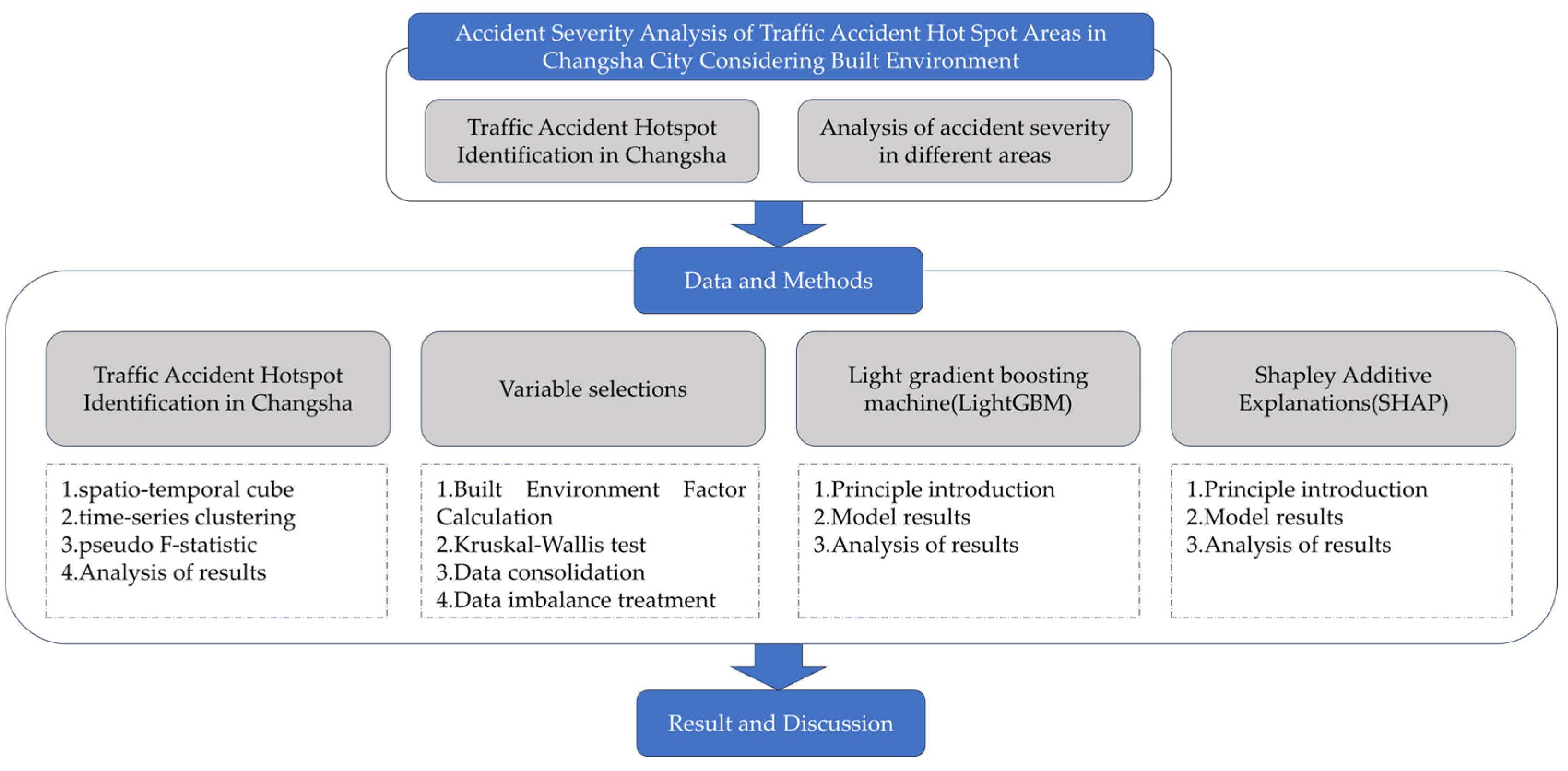
The Technology Roadmap of the article can be obtained as shown in Figure 1 below:
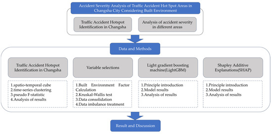
Figure 1.
Technology roadmap.
2. Data Preprocessing
2.1. Traffic Accident Hotspot Identification in Changsha
In this study, Changsha City in Hunan Province, China, serves as the study area, utilizing traffic accident data gathered by the Traffic Police Detachment of the Changsha Municipal Public Security Bureau from 1 January 2017 to 31 December 2019 for hotspot identification analysis. As the traffic police reports solely encompass address descriptions of the accidents, this study preserves 6164 accidents with elevated precision after latitude/longitude conversion.
To precisely account for the temporal characteristics of accident hotspots, we employed Lin’s time-series-based spatio-temporal method for identifying traffic accident hotspots and utilized the spatio-temporal cube in ArcGIS 2022 for time-series clustering [7]. Drawing upon prior research and subsequent parameter fine-tuning, the spatial dimension of the spatio-temporal cube was ultimately designated as 1000 meters, the temporal interval as 3 months, and the clustering attribute as the similarity in the number of periodic accidents.
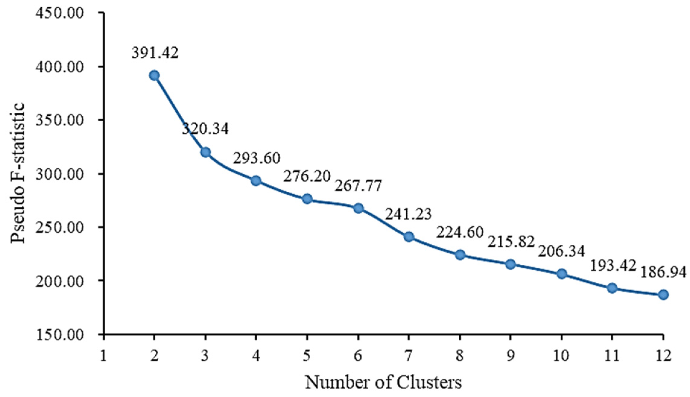
To ascertain the ideal quantity of clustered groupings, this document employs the pseudo F-statistic to evaluate the clustering impact, as depicted in Figure 2. The pseudo F-statistic illustrates the intra-group similarity and inter-group dissimilarity. Greater pseudo F-statistic values indicate improved clustering, amplified distinctions between groups, and heightened intra-group similarity [19]. The findings illustrated in Figure 2 reveal that the pseudo F-statistic peaks at a cluster count of 2, indicating that these particular Changsha traffic accident hotspots are best categorized into two distinct zones: high-accident areas (HAAs) and low-accident areas (LAAs).

Figure 2.
Relation between pseudo-F statistic and cluster number.
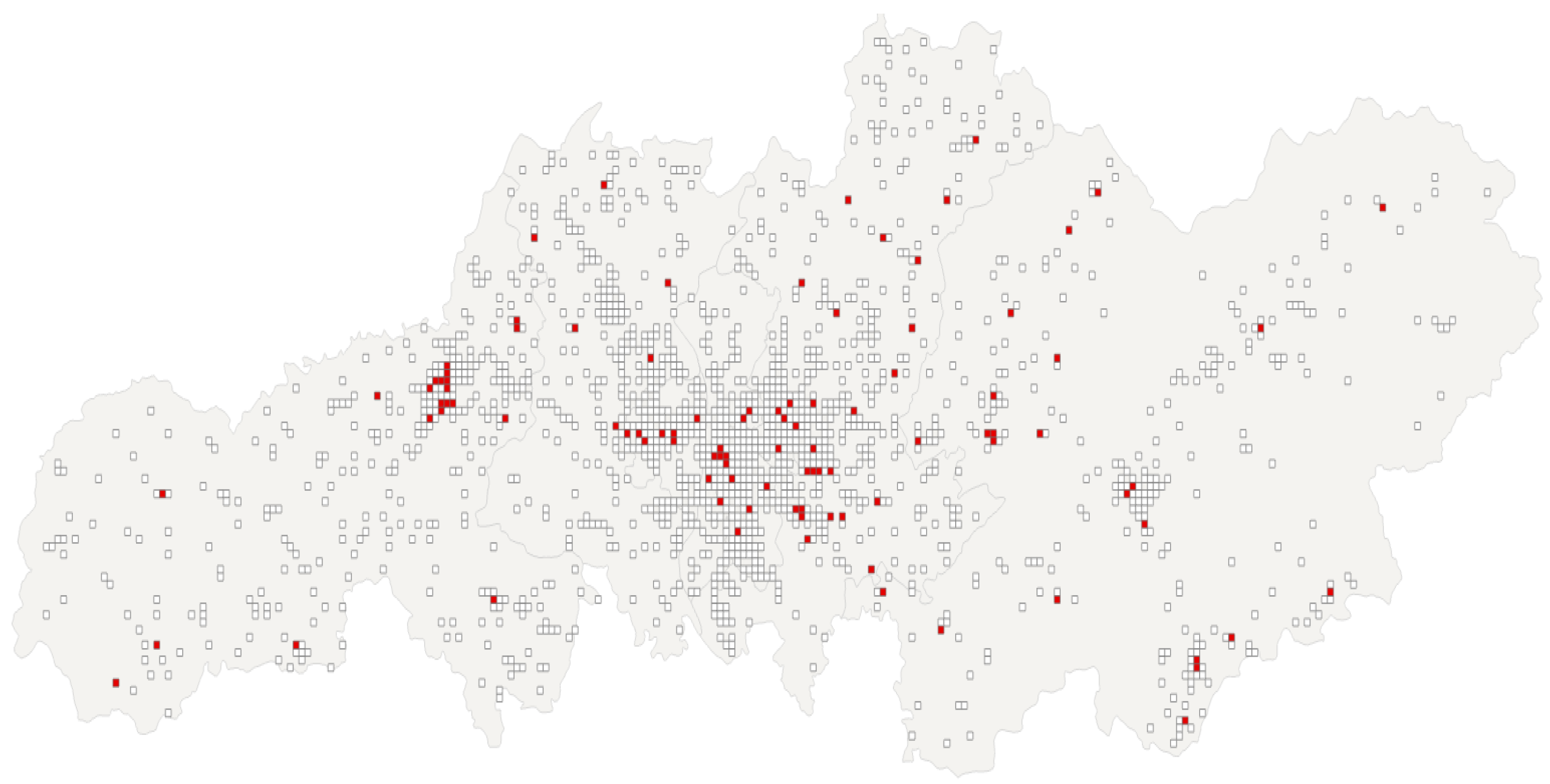
Figure 3 shows the results of identifying road accident hotspots in Changsha. The red squares denote regions of HAAs, comprising 99 blocks with 1811 recorded accidents, while the white squares symbolise LAAs, comprising 1533 blocks with 4353 recorded accidents.
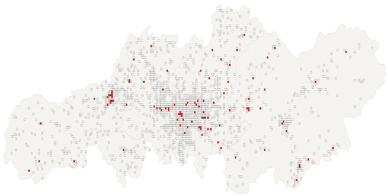
Figure 3.
Results of identifying road accident hotspots in Changsha.
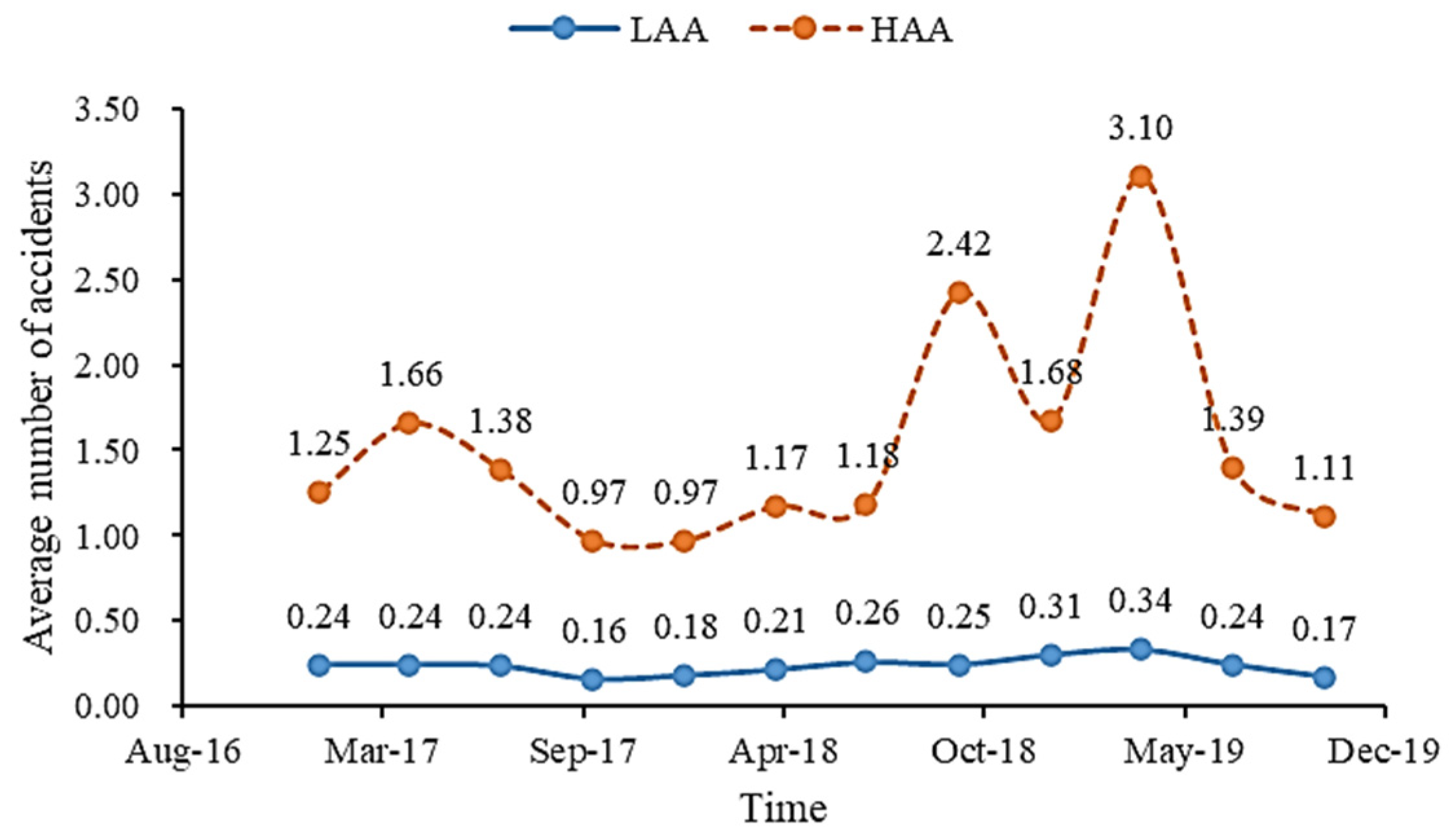
Figure 4 shows the fluctuation in the number of accidents over the different accident area cycles. Within the HAAs, the total number of accidents shows a greater volatility, in contrast to the LAAs, where the fluctuations are more subdued. A comparison of the number of cycles between the two areas shows that the minimum accident frequency in the HAAs is 0.97, while the maximum in the LAAs is 0.34. In particular, the incidence rate in the HAAs is much higher than that in the LAAs.
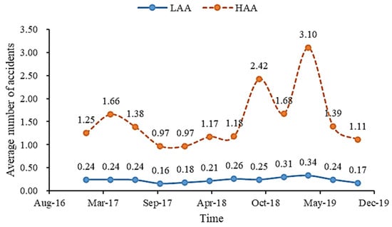
Figure 4.
Number of accidents in different areas.
2.2. Variable Selections
The dataset collected by the Traffic Police Detachment of the Changsha Municipal Public Security Bureau includes more than 60 fields, covering details such as accident descriptions, accident timing, road infrastructure, and environmental conditions, but does not directly include built environment factors. Therefore, this study extracted the Point of Interests (POI) data of the HAAs and LAAs, which cover many types of facility points, such as shopping centres and leisure facilities, etc. This study uses ArcGIS 2022 to quantify the population density, road network density, land use mixing degree, and density of each facility point within the HAAs and LAAs, based on POI data and the ‘5D’ built environment framework [20]. Furthermore, identifying the influences of different built environments in distinct accident areas of the city on accident severity will enable policy makers to initiate urban planning and design interventions and propose more targeted measures to reduce road casualties. Accordingly, this study used the Kruskal–Wallis test to identify differences in built environment factors between HAAs and LAAs. This non-parametric method is suitable for the data structure of this study, as it does not require assumptions of normal distribution and equal variance [21].
Table 1 shows the results of the Kruskal–Wallis test for the built environment factors of the HAAs and LAAs. The test statistic indicates the degree of divergence between the built environment characteristics of the two areas, with a larger value indicating a greater divergence. The p-value indicates the degree of confidence in the results of that test statistic. If the p-value falls below the significance threshold (usually set at 0.05), it can be concluded that there is a difference between the two. As can be seen from Table 1, the p-values for public accessibility, business accessibility, density of greenfield places, and density of residential places are all greater than 0.05. This indicates that there is no significant difference in these factors between the two areas. Consequently, these factors are excluded from the following analyses.

Table 1.
Results of the Kruskal–Wallis test.
Previous research has shown that a thorough understanding of the mechanisms underlying the influences of factors such as accident time, road facilities, and the environment on accident severity is essential for improving road safety [22,23,24,25]. When building the model, accident characteristics should be included in the analysis to provide more comprehensive results. The final combination of accident characteristics and differentiated built environment elements resulted in the detailed variable descriptions in Table 2.
Table 2.
Variable descriptions.
2.3. Data Imbalance Treatment
From Table 2, it can be seen that there is an obvious data imbalance between the accident datasets of the HAAs and LAAs, which will directly affect the training of the model and will lead to a more biased classification towards the majority class and inaccurate classification results. To solve this problem, many researchers use a hybrid sampling method to balance the data. Within this range of techniques, SMOTEENN, which is based on SMOTE and uses the ENN algorithm to meticulously sift the resulting data, has demonstrated its superiority over conventional sampling methods through empirical evidence from several canonical datasets [26]. SMOTEENN was, therefore, used to achieve data equalisation in this paper. The process is described below:
- SMOTE
- (1)
- For each minority class sample, find its K nearest neighbours.
- (2)
- A number of samples are randomly selected for the K nearest neighbours, and a new sample is generated by randomly selecting a point on the line connecting them to their nearest neighbours.
- (3)
- Repeat until balanced.
- ENN
- (1)
- Calculate the majority class sample proportion of its K nearest neighbours for newly generated samples from SMOTE.
- (2)
- If the sample is a minority class sample and has more than 50% of its nearest neighbours in the majority class, remove it.
- (3)
- Integration to generate new data.
After data adjustment by SMOTEENN, the imbalance ratio was reduced from 3.1 to 1.7 and the data imbalance was significantly improved.
3. Methods
3.1. LightGBM
LightGBM (light gradient boosting machine) is an integrated learning model based on gradient boosting tree (GBDT), which was proposed by Ke in 2017 [27]. Compared with models such as GBDT and XGBoost, it discretizes the values of each feature by using a histogram algorithm with a binning method, and then divides the values within a certain range into a certain bin, discretizes the continuous floating-point feature values into k integers, and, at the same time, constructs a histogram of width k instead of the original data, which can search for the optimal segmentation point by calculating the gradient traversal of each bucket. In addition, when calculating the histogram, the histogram of a leaf can be obtained by making a difference between the histogram of its parent node and the histogram of its sibling, and the above improvement can significantly reduce the computational effort as well as the memory occupancy and improve the computation rate.
GBDT [28] and XGBoost [29] models typically use a grow-by-layer strategy during the in-built decision tree growth. This strategy splits leaves of the same layer at the same time by calculating the gain of each node, which has the advantages of good parallelism and easy control of the model complexity, but its efficiency is poor, and it does not discriminate between treating leaves of the same layer and still continues to split the search for leaves with very low splitting gain. LightGBM reduces the error with the same number of splits by using a grow-by-leaf strategy that only splits the leaf with the highest node gain. However, its grow-by-leaf strategy can grow a deeper decision tree, leading to overfitting; LightGBM sets the maximum depth of the tree for this case to prevent overfitting while maintaining a high efficiency.
3.2. SHAP
SHAP (Shapley Additive Explanations) is a machine learning explanation method based on game theory. The core idea is to calculate the contribution of each feature to the model output and then explain the “black box model” at both the global and local levels [30]. When analysing traffic accidents, the use of SHAP values to describe the severity of a traffic accident can be used to efficiently investigate the impacts of various factors on the severity of the accident, thus improving the understanding of the factors that aggravate accident casualties. The specific formula for SHAP is as follows:
Given that the i-th data point in the accident dataset is denoted as xi, the j-th accident characteristic variable of the ith data point is xij, and the predicted value of the model after training is yi, the distribution of SHAP values associated with the model can be represented as:
where ybase denotes the average output of the model in the absence of the input features and f(xij) denotes the SHAP value attributed to the j-th incident feature variable in the i-th sample. The formula for f(xij) is shown below:
where n is the set containing all random feature variables present in sample xi and S is the subset of features composed of all random feature variables of sample xi. v(S) is the sum of the contribution values of the feature variables within the subset S, where is the contribution value of the random feature variable j to the overall model. SHAP values are both positive and negative: a positive value symbolises an increase in the severity of the accident due to the characterised variable, while a negative value indicates a decrease in the severity of the accident due to the characterised variable.
4. Result and Discussion
4.1. Result
The experimental data were divided into test and training sets. In order to ensure the comprehensive use of the data for model training, while preserving sufficient data to evaluate the model’s ability to generalise to unseen data, this paper splits the test set/training set ratio into 70% and 30%, based on lessons learned from previous studies [15]. In this paper, the evaluation metrics commonly used in machine learning were used, including accuracy, precision, recall, f1-score, and area under the curve (AUC). Typically, a model’s performance is considered as excellent if each metric exceeds the 80% threshold [31]. The model constructed from the HAA data showed an accuracy of 95.8%, precision of 96.1%, recall of 97.3%, f1-score of 96.7%, and AUC of 95.3%. The model constructed from the LAA data showed an accuracy of 91.6%, precision of 91.5%, recall of 96.2%, f1-score of 93.8%, and AUC of 89.4%. All of the above exceed the 80% threshold, indicating the overall effectiveness and suitability of the model for further exploration of the key factors influencing accident severity.
4.2. Discussion
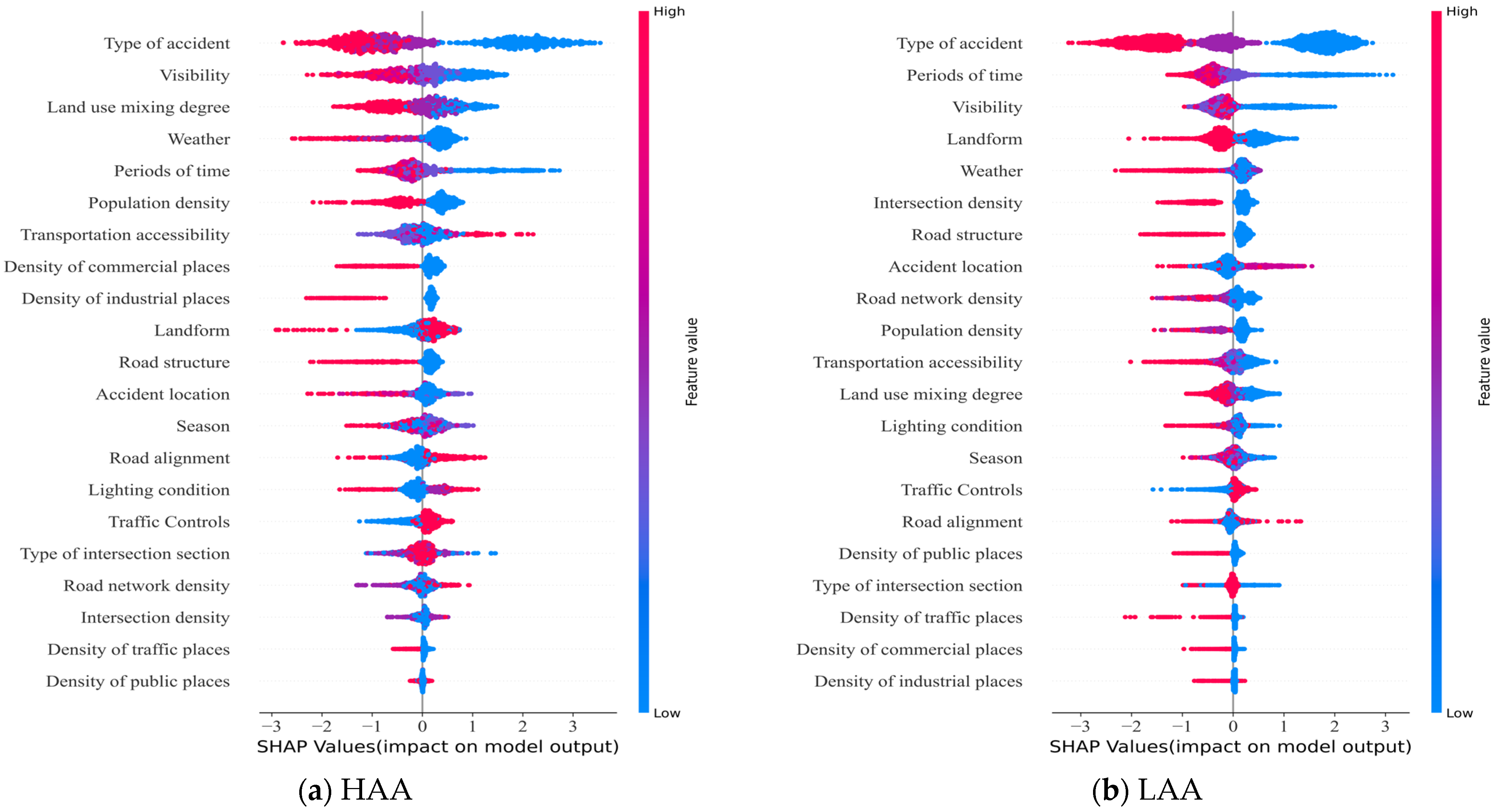
The model uses a summary plot of SHAP values to establish the relationship between the importance of each contributing factor to an incident and its precise impact. Each data point in Figure 5 represents an individual sample of accident data, with the frequency of the data points reflecting the percentage of each characteristic value sampled. The colour scheme represents the coded value of the feature variable, with red indicating higher coded values and blue indicating lower coded values. For example, for the Traffic Controls feature, a low blue value represents 1 (uncontrolled), while a high red value represents 2 (controlled). The horizontal coordinate represents the SHAP value, which quantifies the influence of each feature on the results. The magnitude of the SHAP value indicates the magnitude of this influence.
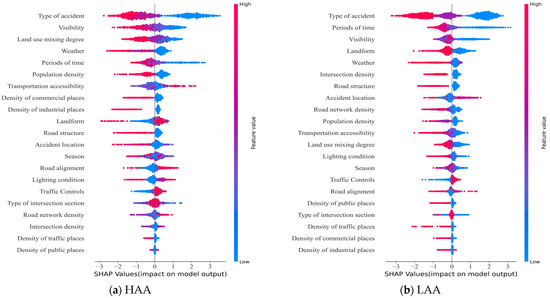
Figure 5.
Summary plot of SHAP values.
As can be seen in Figure 5, there are significant differences in the impacts of accident characteristics and built environment factors on accident severity in different accident areas of the city. In HAAs, type of accident, visibility, land use mixing degree, weather, period of time, and population density are the main influencing factors. In LAAs, type of accident, period of time, visibility, landform, weather, and intersection density are the decisive factors. Despite the differences in the main influencing factors between the different accident zones within the city, there is a consistent trend in the impact of certain factors on the severity of accidents.
Collisions between vehicles and pedestrians and between vehicles and non-motorised vehicles are more likely to result in fatalities, while collisions between vehicles are more likely to result in non-fatal injuries [32]. This is due to the vulnerability of pedestrians and non-motorised users as road users, who lack the protective barriers of motor vehicles and are, therefore, directly exposed to collisions, increasing the likelihood of fatal accidents [33,34].
Visibility shows a trend where increased visibility correlates with a reduced likelihood of a fatal crash. Poor visibility (<50 m) has a positive SHAP value in both the HAA and LAA contexts, indicating a significant escalation in accident severity. Poor visibility limits human vision, giving insufficient time and distance to avoid a collision [7].
The degree of land use mixing shows a pattern in which increased mixing correlates with a reduced impact on fatalities, consistent with the findings of Fatmi [35] and Chen [17]. This can be linked to the fact that increased land use contributes to shorter commuting distances, lower vehicle speeds, and more efficient use of space.
Sunny weather conditions tend to increase the risk of fatal accidents, while other weather conditions reduce the likelihood of fatal accidents. The conclusion differs from subjective perceptions, which may be related to the distribution of accidents. As fewer people venture out in bad weather than on sunny days, the number of such accidents remains comparatively low.
Non-fatal accidents are more likely to occur in the morning, afternoon, and evening, while midnight accidents are more likely to result in fatalities. The reason for this trend is the tendency towards drowsiness and fatigue during the late hours, coupled with a reduction in vehicle and pedestrian traffic. This may encourage drivers to drive more carelessly, leading to increased speeds and an increase in the number of casualties [36].
Population density shows a tendency for the impact of non-fatal accidents to increase progressively with a higher density. This is attributed to the lower speed limits on roads in densely populated regions, thus reducing the likelihood of fatal accidents [37].
The density of commercial places, the density of industrial places, the density of intersections, the density of traffic places, and the density of public places show that the likelihood of non-fatal accidents increases with density. This may be due to the high volume of traffic at these locations, which results in lower speed limits on the roads [38].
Contrasting Figure 5 highlights the presence of certain factors that have different effects in the two models. In order to allow for a more precise comparison of these differences, they are analysed quantitatively using SHAP partial dependency plots.
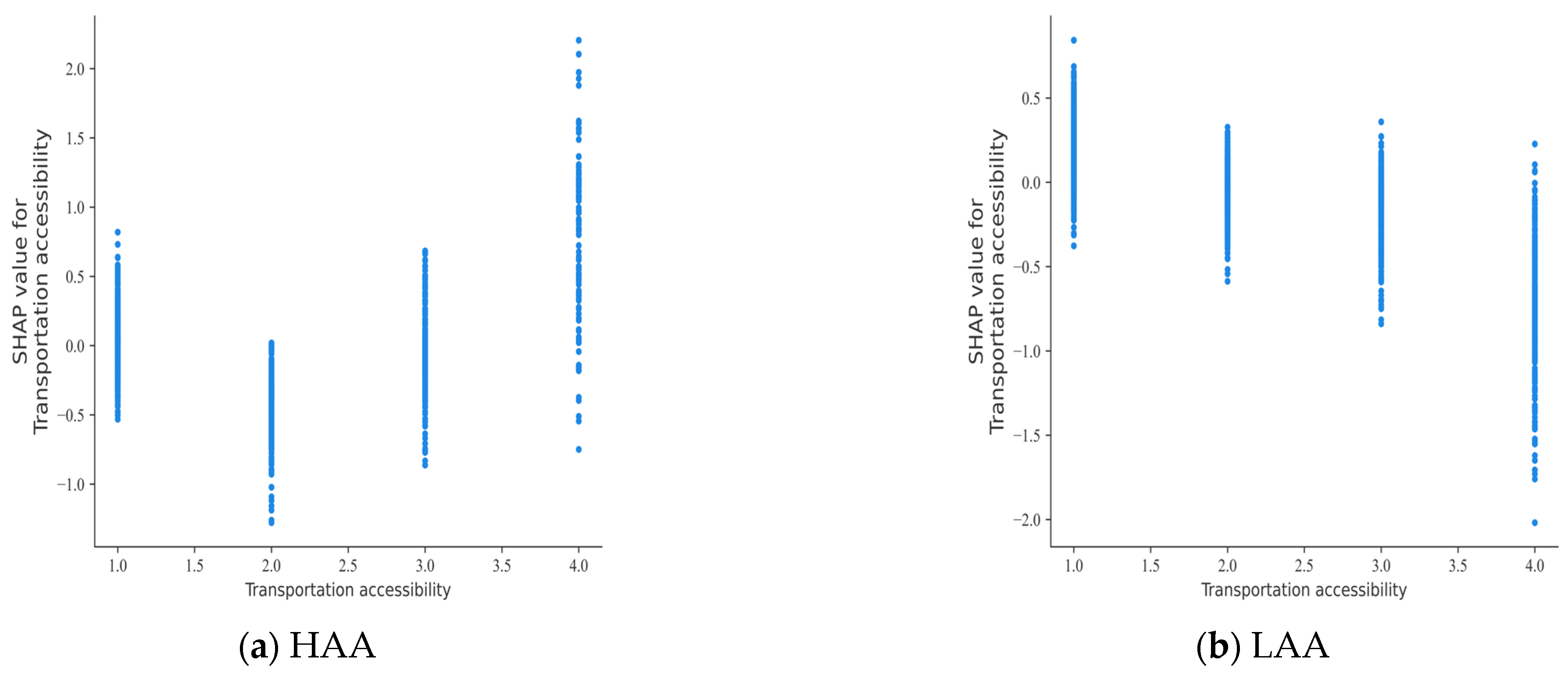
The different effects of built environment factors on the severity of HAA and LAA accidents are shown in Figure 6 and Figure 7. In Figure 6a, it can be seen that, within HAAs, the probability of a fatal accident decreases when the transportation accessibility code value is 2 (678–1658 m). Conversely, as shown in Figure 6b, within LAAs, a lower value of transportation accessibility (indicating proximity to traffic places) corresponds to an increased risk of fatal accidents. This phenomenon may be due to the fact that, in LAAs, an increase in the number of traffic-like places around accidents increases the risk of accidents occurring, leading to more fatal accidents [39].
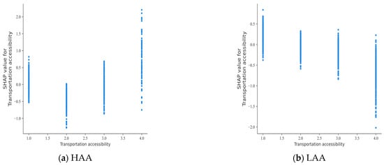
Figure 6.
SHAP partial dependence plot for transportation accessibility.
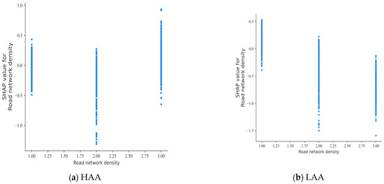
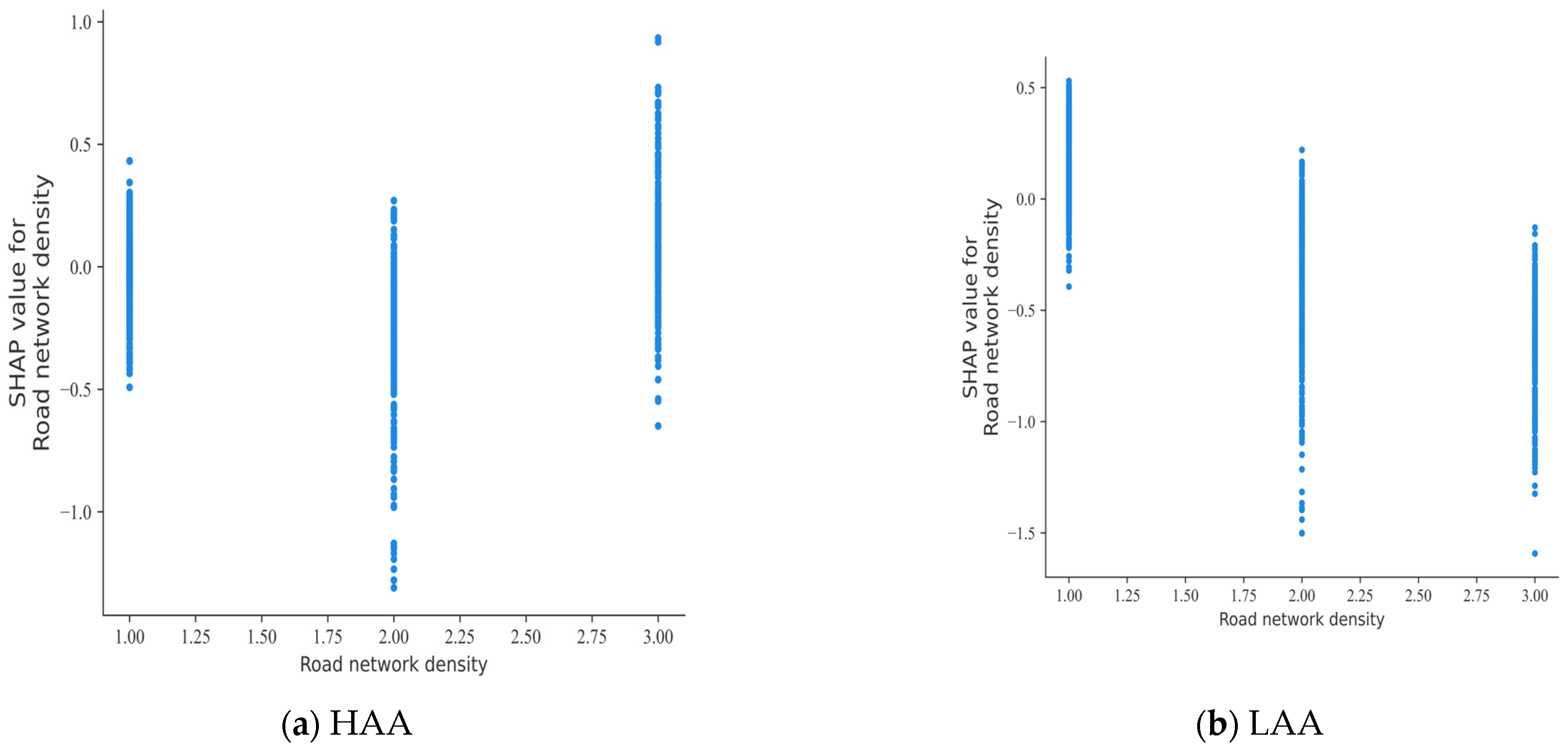
Figure 7.
SHAP partial dependence plot for road network density.
Figure 7 shows the SHAP partial dependency plot under the influence of road network density. Within HAAs, there is no discernible correlation between road network density and accident severity. Conversely, within LAAs, there is a tendency for road casualties to decrease as the road network density increases [40].
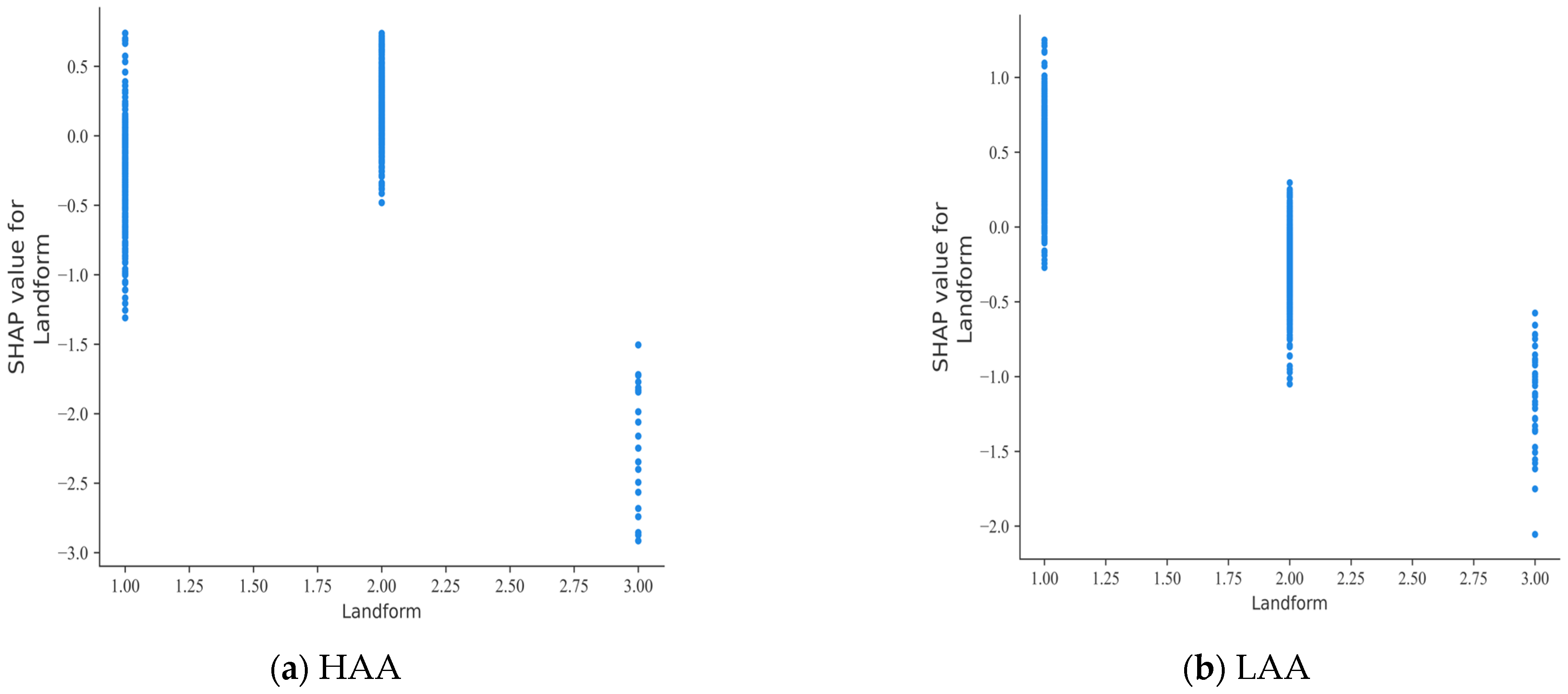
The influences of accident characterisation factors on the severity of accidents in different regions are illustrated in Figure 8 and Figure 9. Figure 8 shows the effect of landform on accident severity. In HAAs, the presence of plain and mountainous terrain generally reduces the severity of accidents, while hilly terrain can lead to increased accident casualties. This phenomenon can be attributed to drivers’ reduced visibility due to the undulating nature of hilly terrain [41]. Conversely, in LAAs, hilly and mountainous terrain reduces the likelihood of fatal accidents, while accidents in plain areas are more likely to be fatal.
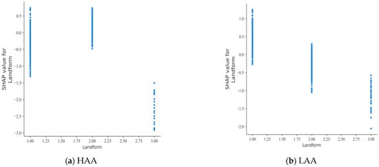
Figure 8.
SHAP partial dependence plot for landform.
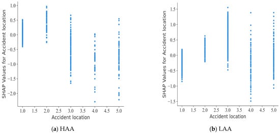
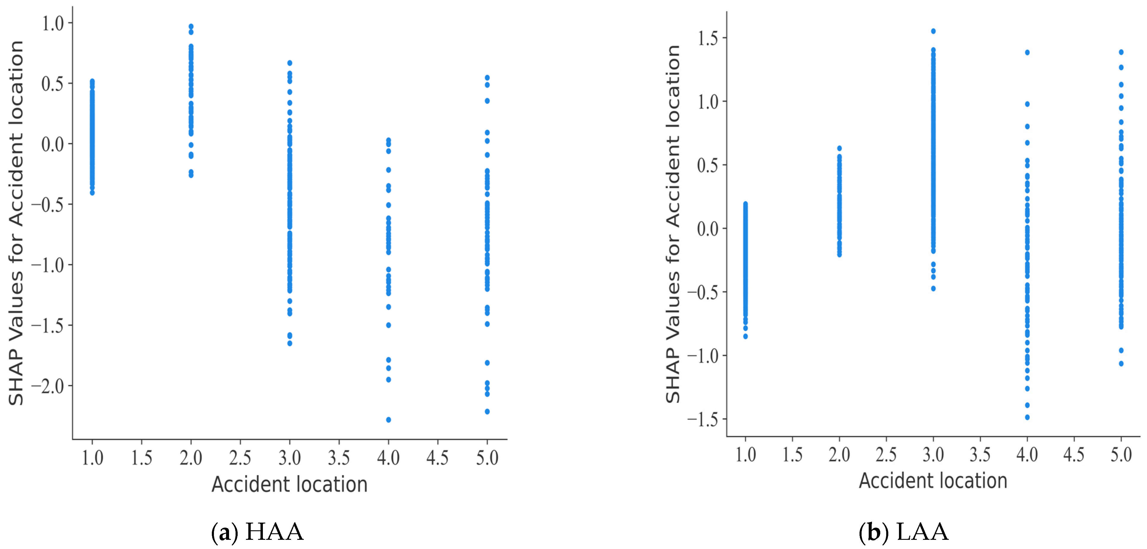
Figure 9.
SHAP partial dependence plot for accident location.
Figure 9 shows the differences in the impact of the location of the accident on the severity of the accident. In high-accident areas, accidents on motorised and non-motorised roads are often fatal, while accidents on motorised and non-motorised roads, footpaths, and other locations are predominantly non-fatal. Conversely, this pattern follows an opposite trajectory in regions with low accident rates. This dynamic is closely related to the spatial arrangement of the high-crash areas, which are mainly concentrated in the main urban areas of Changsha, where speed limits on motorised and non-motorised roads, footpaths, and alternative locations are lower, thereby reducing the risk of fatal crashes.
5. Conclusions
In order to explore the potential impacts of built environment factors on accident severity within traffic accident hotspots, this paper first classified the traffic accident hotspots in Changsha City using a time-series clustering method. Then, relevant built environment factors were extracted for the identified accident hotspots, and the LightGBM and SHAP models were used to investigate the differences in accident severity between different urban accident zones under the influence of accident characteristics and differentiated built environment factors.
- (1)
- In different accident areas within the city, the features influencing accident severity and the built environment factors differ. In HAAs, the primary influencing factors include type of accident, visibility, land use mixing degree, weather, period of time, and population density. Conversely, in LAAs, the key factors revolve around type of accident, period of time, visibility, landform, weather, and intersection density.
- (2)
- The importance of certain factors in influencing the severity of accidents varies between different accident hotspots. However, the overall trend in their impact on accidents remains consistent. With regard to factors related to accident characteristics, vehicle–pedestrian accidents, vehicle–non-motorized vehicle accidents, poor visibility, and midnight driving exacerbate accident severity. Among the factors related to the built environment, an increase in the land use mixing degree, population density, density of commercial places, density of industrial places, density of intersections, density of traffic places, and density of public places correlates positively with a decrease in fatal accidents.
- (3)
- There are significant differences in the trends of the impacts of certain factors on accident severity between different urban accident areas. With regard to the built environment, transportation accessibility and road network density exhibit varying effects on accident severity. Meanwhile, differences in landform and accident location lead to an inconsistent impact on accident severity in terms of accident characteristics.
Author Contributions
Conceptualization, methodology, formal analysis, writing—original draft, R.Y.; resources, conceptualization, supervision, validation, writing—review and editing, L.H.; implemented the editing work, J.L.; implemented the editing work, N.L. All authors have read and agreed to the published version of the manuscript.
Funding
This work was supported by the National Natural Science Funds for Distinguished Young Scholar (Grant No. 52325211), the National Natural Science Foundation of China (Grant Nos. 52172399 and 52372348), the Science and Technology Innovative Research Team in Higher Educational Institutions of Hunan Province and Natural Science Foundation of Changsha (Grant No. KQ2208235).
Institutional Review Board Statement
Not applicable.
Informed Consent Statement
Not applicable.
Data Availability Statement
The detailed accident data cannot be disclosed due to confidentiality agreements.
Conflicts of Interest
The authors declare that they have no known competing financial interests or personal relationships that could have appeared to influence the work reported in this paper.
References
- Ding, C.; Chen, P.; Jiao, J. Non-linear effects of the built environment on automobile-involved pedestrian crash frequency: A machine learning approach. Accid. Anal. Prev. 2018, 112, 116–126. [Google Scholar] [CrossRef]
- Chen, P.; Sun, F.; Wang, Z.; Gao, X.; Jiao, J.; Tao, Z. Built environment effects on bike crash frequency and risk in Beijing. J. Saf. Res. 2018, 64, 135–143. [Google Scholar] [CrossRef] [PubMed]
- Yoon, J.; Lee, S. Spatio-temporal patterns in pedestrian crashes and their determining factors: Application of a space-time cube analysis model. Accid. Anal. Prev. 2021, 161, 106291. [Google Scholar] [CrossRef] [PubMed]
- Afghari, A.P.; Haque, M.M.; Washington, S. Applying a joint model of crash count and crash severity to identify road segments with high risk of fatal and serious injury crashes. Accid. Anal. Prev. 2020, 144, 105615. [Google Scholar] [CrossRef]
- Ghezelbash, S.; Ghezelbash, R.; Kalantari, M. Developing a spatio-temporal interactions model for car crashes using a novel data-driven AHP-TOPSIS. Appl. Geogr. 2024, 162, 103151. [Google Scholar] [CrossRef]
- Hu, L.; Wu, X.; Huang, J.; Peng, Y.; Liu, W. Investigation of clusters and injuries in pedestrian crashes using GIS in Changsha, China. Saf. Sci. 2020, 127, 104710. [Google Scholar] [CrossRef]
- Lin, N.; Hu, L.; Lin, M.; Peng, H. Black spot identification and analysis of traffic accidents based on time series clustering. J. Chang. Univ. Sci. Technol. Nat. Sci. 2023, 20, 45–54. [Google Scholar]
- Lu, H.; Luo, S.; Li, R. GlS-based Spatial Patterns Analysis of Urban Road Traffic Crashes in Shenzhen. China J. Highw. Transp. 2019, 32, 156–164. [Google Scholar]
- Wang, X.; Zhang, X.; Pei, Y. A systematic approach to macro-level safety assessment and contributing factors analysis considering traffic crashes and violations. Accid. Anal. Prev. 2024, 194, 107323. [Google Scholar] [CrossRef] [PubMed]
- Al Hamami, M.; Matisziw, T.C. Measuring the spatiotemporal evolution of accident hot spots. Accid. Anal. Prev. 2021, 157, 106133. [Google Scholar] [CrossRef] [PubMed]
- Shin, S.; Choo, S. Influence of Built Environment on Micromobility–Pedestrian Accidents. Sustainability 2022, 15, 582. [Google Scholar] [CrossRef]
- Bi, H.; Li, A.; Zhu, H.; Ye, Z. Bicycle safety outside the crosswalks: Investigating cyclists’ risky street-crossing behavior and its relationship with built environment. J. Transp. Geogr. 2023, 108, 103551. [Google Scholar] [CrossRef]
- Lym, Y.; Chen, Z. Influence of built environment on the severity of vehicle crashes caused by distracted driving: A multi-state comparison. Accid. Anal. Prev. 2021, 150, 105920. [Google Scholar] [CrossRef] [PubMed]
- Lee, S.; Yoon, J.; Woo, A. Does elderly safety matter? Associations between built environments and pedestrian crashes in Seoul, Korea. Accid. Anal. Prev. 2020, 144, 105621. [Google Scholar] [CrossRef] [PubMed]
- Wang, J.; Ji, L.; Ma, S.; Sun, X.; Wang, M. Analysis of Factors Influencing the Severity of Vehicle-to-Vehicle Accidents Considering the Built Environment: An Interpretable Machine Learning Model. Sustainability 2023, 15, 12904. [Google Scholar] [CrossRef]
- Yang, C.; Chen, M.; Yuan, Q. The application of XGBoost and SHAP to examining the factors in freight truck-related crashes: An exploratory analysis. Accid. Anal. Prev. 2021, 158, 106153. [Google Scholar] [CrossRef] [PubMed]
- Chen, P.; Shen, Q. Identifying high-risk built environments for severe bicycling injuries. J. Saf. Res. 2019, 68, 1–7. [Google Scholar] [CrossRef]
- Ji, X.; Qiao, X.; Pu, Y.; Lu, M.; Hao, J. Influence mechanism of built environment around subway station on traffic accident risk. China Saf. Sci. J. 2022, 32, 162–170. [Google Scholar]
- Joshi, M.Y.; Rodler, A.; Musy, M.; Guernouti, S.; Cools, M.; Teller, J. Identifying urban morphological archetypes for microclimate studies using a clustering approach. Build. Environ. 2022, 224, 109574. [Google Scholar] [CrossRef]
- Ewing, R.; Cervero, R. Travel and the built environment: A synthesis. Transp. Res. Rec. 2001, 1780, 87–114. [Google Scholar] [CrossRef]
- Clark, J.S.C.; Kulig, P.; Podsiadło, K.; Rydzewska, K.; Arabski, K.; Białecka, M.; Safranow, K.; Ciechanowicz, A. Empirical investigations into Kruskal-Wallis power studies utilizing Bernstein fits, simulations and medical study datasets. Sci. Rep. 2023, 13, 2352. [Google Scholar] [CrossRef] [PubMed]
- Umer, M.; Sadiq, S.; Ishaq, A.; Ullah, S.; Saher, N.; Madni, H.A. Comparison Analysis of Tree Based and Ensembled Regression Algorithms for Traffic Accident Severity Prediction. arXiv 2020, arXiv:2010.14921. [Google Scholar]
- Zeng, J.; Qian, Y.; Yin, F.; Zhu, L.; Xu, D. A multi-value cellular automata model for multi-lane traffic flow under lagrange coordinate. Comput. Math. Organ. Theory 2022, 28, 178–192. [Google Scholar] [CrossRef]
- Glimm, J.; Fenton, R.E. An accident-severity analysis for a uniform-spacing headway policy. IEEE Trans. Veh. Technol. 1980, 29, 96–103. [Google Scholar] [CrossRef]
- Jia, L.; Cheng, P.; Yu, Y.; Chen, S.-H.; Wang, C.-X.; He, L.; Nie, H.-T.; Wang, J.-C.; Zhang, J.-C.; Fan, B.-G.; et al. Regeneration mechanism of a novel high-performance biochar mercury adsorbent directionally modified by multimetal multilayer loading. J. Environ. Manag. 2023, 326, 116790. [Google Scholar] [CrossRef] [PubMed]
- Yan, Y.; Dai, T.; Zhang, Y.; Zhao, S.; Zhang, Y. Neighborhood-aware lmbalanced Oversampling. J. Chin. Comput. Syst. 2021, 42, 1360–1370. [Google Scholar]
- Ke, G.; Meng, Q.; Finley, T.; Wang, T.; Chen, W.; Ma, W.; Ye, Q.; Liu, T.-Y. Lightgbm: A highly efficient gradient boosting decision tree. In Proceedings of the 31st International Conference on Neural Information Processing Systems, Long Beach, CA, USA, 4–9 December 2017; pp. 3149–3157. [Google Scholar]
- Friedman, J.H. Greedy function approximation: A gradient boosting machine. Ann. Stat. 2001, 29, 1189–1232. [Google Scholar] [CrossRef]
- Chen, T.; Guestrin, C. Xgboost: A scalable tree boosting system. In Proceedings of the 22nd ACM Sigkdd International Conference on Knowledge Discovery and Data Mining, San Francisco, CA, USA, 13–17 August 2016; pp. 785–794. [Google Scholar]
- Lundberg, S.M.; Lee, S.I. A unified approach to interpreting model predictions. In Proceedings of the 31st International Conference on Neural Information Processing Systems, Long Beach, CA, USA, 4–9 December 2017; pp. 4768–4777. [Google Scholar]
- Wei, T.; Zhu, T.; Lin, M.; Liu, H. Predicting and factor analysis of rider injury severity in two-wheeled motorcycle and vehicle crash accidents based on an interpretable machine learning framework. Traffic Inj. Prev. 2024, 25, 194–201. [Google Scholar] [CrossRef] [PubMed]
- Jeong, H.; Kim, I.; Han, K.; Kim, J. Comprehensive analysis of traffic accidents in seoul: Major factors and types affecting injury severity. Appl. Sci. 2022, 12, 1790. [Google Scholar] [CrossRef]
- Li, Y.; Fan, W.D. Modelling severity of pedestrian-injury in pedestrian-vehicle crashes with latent class clustering and partial proportional odds model: A case study of North Carolina. Accid. Anal. Prev. 2019, 131, 284–296. [Google Scholar] [CrossRef]
- Qian, Q.; Shi, J. Comparison of injury severity between E-bikes-related and other two-wheelers-related accidents: Based on an accident dataset. Accid. Anal. Prev. 2023, 190, 107189. [Google Scholar] [CrossRef] [PubMed]
- Fatmi, M.R.; Habib, M.A. Modeling vehicle collision injury severity involving distracted driving: Assessing the effects of land use and built environment. Transp. Res. Rec. 2019, 2673, 181–191. [Google Scholar] [CrossRef]
- Zhang, G.; Yau, K.K.W.; Zhang, X.; Li, Y. Traffic accidents involving fatigue driving and their extent of casualties. Accid. Anal. Prev. 2016, 87, 34–42. [Google Scholar] [CrossRef] [PubMed]
- Ewing, R.; Dumbaugh, E. The built environment and traffic safety: A review of empirical evidence. J. Plan. Lit. 2009, 23, 347–367. [Google Scholar] [CrossRef]
- Prato, C.G.; Kaplan, S.; Patrier, A.; Rasmussen, T.K. Considering built environment and spatial correlation in modeling pedestrian injury severity. Traffic Inj. Prev. 2018, 19, 88–93. [Google Scholar] [CrossRef] [PubMed]
- Yasmin, S.; Eluru, N. Latent segmentation based count models: Analysis of bicycle safety in Montreal and Toronto. Accid. Anal. Prev. 2016, 95, 157–171. [Google Scholar] [CrossRef]
- Ji, X.; Qiao, X. Nonlinear Influence of Built Environment on Pedestrian Traffic Accident Severity. J. Transp. Syst. Eng. Inf. Technol. 2023, 23, 314–323. [Google Scholar]
- Hosseinpour, M.; Yahaya, A.S.; Sadullah, A.F. Exploring the effects of roadway characteristics on the frequency and severity of head-on crashes: Case studies from Malaysian Federal Roads. Accid. Anal. Prev. 2014, 62, 209–222. [Google Scholar] [CrossRef] [PubMed]
Disclaimer/Publisher’s Note: The statements, opinions and data contained in all publications are solely those of the individual author(s) and contributor(s) and not of MDPI and/or the editor(s). MDPI and/or the editor(s) disclaim responsibility for any injury to people or property resulting from any ideas, methods, instructions or products referred to in the content. |
© 2024 by the authors. Licensee MDPI, Basel, Switzerland. This article is an open access article distributed under the terms and conditions of the Creative Commons Attribution (CC BY) license (https://creativecommons.org/licenses/by/4.0/).