
A Hybrid Approach Based on Consensus Decision Making for Green Supplier Selection in Automotive Industry


Department of Mathematics, Yildiz Technical University, Istanbul 34220, Türkiye
Sustainability 2024, 16(7), 3096; https://doi.org/10.3390/su16073096
Submission received: 22 February 2024
/
Revised: 3 April 2024
/
Accepted: 4 April 2024
/
Published: 8 April 2024
Abstract
:With increased global commerce, businesses must manage their supply chains while taking into account not only costs but also environmental implications. The decision-making of Green Supplier Selection (GSS) is a strategic priority for companies to survive in challenging market conditions and to effectively and sustainably manage their supply chains in the increasingly polluted and resource-depleted world. Environmental sustainability can be enhanced with the appropriate criteria when choosing green suppliers. Based on these motivations, it is necessary to determine the correct criteria, classify the chosen criteria and employ an effective evaluation method in the GSS process. In particular, evaluating each criterion at its own level is of strategic importance. In this paper, the GSS model, handled by group decision-making, is constructed with multi-sub-criteria to increase the competitive advantage of businesses in challenging market conditions for the purpose of ensuring a sustainable future. A novel hybrid methodology of the Interval Type-2 Fuzzy (IT2F) Analytical Hierarchy Process (AHP) and IT2F Technique for Order of Preference by Similarity to Ideal Solution (TOPSIS) is presented for the GSS model to deal with uncertainty. This study provides decision-makers with an effective method that performs fuzzy calculations at all steps until a solution is found, especially in areas that may have a complex hierarchical structure, such as the automotive industry. In the proposed method, unlike most studies in the literature, if a criterion has sub-criteria (or multi-sub-criteria) in the hierarchy considered, each criterion is evaluated with other criteria at its own level, without the need for all other criteria to have sub-criteria (or multi-sub-criteria). The effectiveness of the proposed method has been demonstrated by testing it with an application taken from the automotive industry with a complex-structured multi-level hierarchy. Additionally, sensitivity analysis has been conducted to assess the impact of changes in subjective input by means of scenarios.
1. Introduction
Global warming, air pollution, water pollution, and shortage of resources are all challenges caused by humans. Environmental conservation should be a major concern for everyone in order to protect the continuation of life in this world and to leave a habitable planet for future generations. Green resources, in particular, should be used by both producers and consumers to be able to achieve this. The ability of nature to maintain itself will grow as the consumption of green resources increases. From this perspective, green supply chain management is becoming remarkably vital and required for businesses seeking to accomplish environmental sustainability goals in an increasingly dirty and resource-depleted world. GSS, part of the green supply chain, is a critical process that helps companies choose eco-friendly suppliers in order to reduce their influence on the environment while delivering their products and services. The performance criteria were identified to examine the GSS process, and methods were offered for efficient supplier selection from an ecologic point of view by Noci [1]. Govindan et al. [2] presented an extensive survey of the published research about GSS from 1997 to 2011. Many GSS problems that involve qualitative and quantitative factors from different industries can be solved by Multi-Criteria Decision-Making (MCDM) techniques. Tronnebati et al. [3] analyzed ten studies examining 1098 research papers in academic journals between 1990 and 2020 to assess which techniques are most often utilized and more efficient for solving GSS problems. The fact that AHP and TOPSIS are the most commonly utilized MCDM techniques in GSS studies with regard to the findings has strengthened the motivation of this study.
In the modern business world, companies face complicated and multidimensional problems in their decision-making processes. Businesses must now make comprehensive and sustainable decisions by taking into account environmental, social, economic, and strategic issues instead of making decisions based just on financial data. At this juncture, MCDM techniques offer powerful tools to analyze, evaluate, and optimize complicated problems. Determining the appropriate MCDM techniques and effectively applying them play a critical role in establishing companies’ future strategies. Many studies in the literature utilize AHP and TOPSIS, the most commonly used methods in decision-making processes. Although it is not possible to refer to all the studies, some recently published articles in different research areas based on AHP, TOPSIS, and the AHP-TOPSIS methods obtained by integrating them are mentioned in the following. Using the example of the automotive industry in Pakistan, Dweiri et al. [4] presented a two-hierarchical decision support model for supplier selection with AHP and performed a sensitivity analysis to control the soundness of the decision. Barrios et al. [5] presented a hybrid AHP-TOPSIS model with hierarchical structure and sub-criteria to choose the most suitable tomography equipment. Yu and Hou [6] discussed a GSS problem for an automobile-producing firm in Qingdao via AHP. Zhu et al. [7] offered a framework that is applied in Nanjing, China, as a case study for evaluating the relative performances of multiple neighborhood regeneration projects with the AHP-TOPSIS method. Navarro et al. [8] created a mathematical structure for supplier selection in the industry of wood fiber and applied the AHP-TOPSIS method as a software of Visual Basic and Microsoft Excel for the solution. James et al. [9] applied a hybrid methodology of AHP and the TOPSIS algorithm in order to rank original equipment manufacturer chassis and select the proper chassis for the bus fleet. Gitelman and Kozhevnikov [10] promoted the necessity of merging the transition to low-carbon energy sources with the modernization of the energy industry to reduce technological, financial, and organizational risks. Zeng and Li [11] used a combined model consisting of AHP and TOPSIS to examine the present state of natural gas security in twenty-seven EU nations using several factors.
Another incontrovertible issue is that since real-world data and conditions are often uncertain, incomplete, or subjective, fuzzy numbers emerge as a powerful tool to address and model uncertainties in decision-making processes. Kannan et al. [12] provided an FTOPSIS-based framework for a Brazilian electronics company’s GSS. Keshavarz Ghorabaee et al. [13] presented an extensive survey of the literature on fuzzy GSS from 2001 to 2016. Wang Chen et al. [14] evaluated a GSS problem in the industry of luminance enhancement film with Fuzzy TOPSIS (FTOPSIS)-Fuzzy AHP (FAHP). Samanlioglu et al. [15] solved a staff selection problem in the information technology office of a dairy firm located in Türkiye by combining FTOPSIS and FAHP with extent analysis. Jain et al. [16] used combined FAHP and FTOPSIS methods to address a selection of headlight supplier problems for an Indian car firm. Venkatesh et al. [17] handled a real case about a supplier partner decision for continuous-aid procurement in humanitarian operations and reached a solution combining FAHP and FTOPSIS. Pehlivan et al. [18] chose the best players for the Turkish National Football Team via the integrated FTOPSIS-FAHP technique. Li et al. [19] constructed an expanded TOPSIS technique for sustainable supplier selection based on the cloud model theory and the rough set theory with fuzzy numbers. In the study of Nasrollahi et al. [20], they examined the greenhouses in terms of heat and saving energy by determining the best approach to economize through the FAHP-FTOPSIS. Ekmekcioğlu et al. [21] conducted a risk analysis of the natural flood disaster for the metropolitan city of Istanbul by benefitting from FAHP and TOPSIS. Yildizbasi and Arioz [22] worked on a GSS problem by using the big data analysis and FAHP-FTOPSIS methodologies collectively. Bhattacherjee et al. [23] investigated the features of the personnel selection problem with the views of many experts in different positions and solved it by FAHP-FTOPSIS. Bozanic et al. [24] studied the modification of FAHP to address the issue of selecting navigation routes for vessels in flooded areas based on assessing the risk associated with each potential course. By employing an integrated methodology that Ghazvinian et al. [25] verified through the utilization of FTOPSIS and structural equation modeling, they assessed GSS in an automotive industry case study.
Interval Type-2 Fuzzy Numbers (IT2FNs) assist in producing more precise and realistic results as they can capture the uncertainty of an event in more detail, both in terms of its boundaries and degrees (how uncertain a situation is). IT2FNs, which contain a great deal more information than traditional fuzzy numbers, are commonly combined with MCDM techniques to improve realism and application simplicity. Erdoğan and Kaya [26] used IT2F AHP-IT2F TOPSIS together to select the optimal location for a nuclear plant to be built in Türkiye. Mousakhani et al. [27] provided a novel framework for the GSS problem utilizing IT2F TOPSIS and a group decision-making technique, taking into account the opinions of priority experts on the relative relevance of criteria, and implemented the method to an automotive battery production case in Iran. Celik and Akyuz [28] presented a combination of IT2F AHP and TOPSIS for the purpose of choosing the optimal ship loader designed to load the transportation ships. In the research of Alegoz and Yapicioglu [29], they studied a supplier selection decision by integrating IT2F AHP and FTOPSIS along with the goal programming. Wu et al. [30] evaluated the sustainability performances of hydrogen deposits from the wind turbines via AHP-TOPSIS with an IT2F structure. Mathew et al. [31] worked on a strategic decision problem for maintenance with IT2F AHP-TOPSIS and conducted sensitivity analysis along with an application. Kiracı and Akan [32] employed IT2F AHP-TOPSIS in the selection of a plane for the commercial transportation industry. Yılmaz and Kabak [33] benefitted from IT2F-based AHP-TOPSIS in order to rank the distribution centers and suggest decision support models for various situations in case of an earthquake in Istanbul. Meniz and Tiryaki [34] assessed mobile applications using IT2F AHP. Ecer [35] presented an IT2F AHP model that employed a defuzzification strategy at the intermediate level to solve a GSS problem and was tested in a home appliance company. Sari and Tüysüz [36] evaluated the risk assessment of occupations via a novel AHP-TOPSIS technique under IT2F during COVID-19.
Although a lot of research has been conducted on the subject of GSS literature, it is clear that the expansions of decision-making procedures in the framework of IT2FNs have received little attention, i.e., no studies have been conducted on this topic. To the best of the authors’ knowledge, no research yet offers AHP-TOPSIS in the framework of IT2FNs in the GSS problem and in the assessment of the green supply chain. As a crucial aspect of the decision-making process, the authors have opted for the AHP technique, a fundamental and efficient algorithm, to determine the priority of the importance weights of the criteria. Following this, the TOPSIS methodology has been utilized to rank the alternatives. In this study, the authors addressed the GSS problem for a sustainable future by using IT2FNs, which are extremely successful in reflecting uncertainty. IT2FNs, which indicate the uncertainty of events in more detail regarding both boundaries and degrees, are combined with the AHP-TOPSIS hybrid technique to provide more realistic results and improve application simplicity. Moreover, in contrast to the hybrid method presented, defuzzification methods are implemented to attain the optimum solution before proceeding to the final step of the problem solution in the studies carried out with IT2FN in the literature. Using crisp numbers before the last stage of the operation diminishes the efficacy of IT2FNs. Due to the fact that defuzzification has been only implemented during the final sorting phase in the method, the benefits of employing fuzzy numbers have persisted in the subsequent stages. Therefore, it is clear that the research will significantly impact the literature. This paper’s primary scientific contributions can be stated as follows.
- A comprehensive GSS model with a realistically detailed structure and multi-level hierarchy is enhanced.
- A novel hybrid IT2F AHP-TOPSIS method that performs fuzzy calculations at all steps to solve the GSS problem is presented to fill the gap in the literature.
- The method evaluates each criterion (sub-criterion or multi-sub-criterion) with other criteria at its own level.
- The method provides the decision maker with an evaluation that increases dependability through group decision-making.
- With a green perspective, an application is performed in the automotive industry.
- Sensitivity analysis is carried out to monitor the fluctuations of the alternatives in the overall rankings with the scenarios created by modifying the importance valuations.
The remaining portions of the study are structured as follows. The definitions and preliminary information are provided in Section 2.1. The technique for the solution of the GSS model is described in Section 2.2. Section 3 provides a GSS application in the automotive industry, the comparison of results, and the sensitivity analysis. Lastly, Section 4 includes conclusions and future directions.
2. Methodology
2.1. Mathematical Preliminaries
In this section, some definitions for the IT2FN structure will be given prior to the hybrid technique of IT2F AHP-TOPSIS.
Definition 2:
Summation operation for two IT2FNs and is defined as [38]:
Definition 3:
Multiplication operation between two IT2FNs and is defined as [37]:
Definition 4:
Multiplication of scalar and IT2FN is defined as [37]:
Definition 5:
The inverse of an IT2FN is defined by [39]:
Definition 6:
For an IT2FN , n-th degree root is defined by [39]:
Definition 7:
The defuzzified equivalent of the IT2FN is described by [39]:
Definition 8:
2.2. The Proposed Methodology
In this part, integration of the IT2F AHP designed for multi-level hierarchies and the IT2F TOPSIS proposed to handle IT2FNs more efficaciously will be presented. In the hybrid method, IT2F AHP and IT2F TOPSIS determine the IT2F weight vector that will be utilized in subsequent stages and the final ranking of the alternatives, respectively. First of all, it is emphasized that the geometric mean is used in the AHP portion of the hybrid method due to its ability to handle multiplicative relationships and reduce the effect of extreme values. Additionally, in the TOPSIS portion of the hybrid method, the arithmetic mean is preferred to the geometric mean because it allows the inclusion of operations involving zeros, which may be necessary in some cases.
Step 1:
An appropriate decision hierarchy is established for the problem by obtaining experts with varying viewpoints. Considering this hierarchy, Pairwise Comparison Matrices (PCMs) are constructed using Definition 5, where criteria are compared with each other, and Decision Matrices (DMs) are constructed, where alternatives are rated individually for all criteria by every decision maker.
Step 2:
IT2F PCMs are defuzzified in order to obtain the corresponding crisp reciprocal matrices, and consistency analysis is performed for these matrices. Decision makers re-evaluate the pairwise comparisons for inconsistent matrices. If all matrices are consistent, move on to the next step [39].
Step 3:
Step 4:
The geometric means of each row of the average PCMs are computed with Definitions 3, 5, and 6. Afterward, levelly normalized weights are found using Definitions 3 and 5:
Here, T is defined as the number of criteria at the current hierarchy level [39].
Step 5:
To find fully normalized criteria weights , meaning normalized criteria weights regarding the whole hierarchy, sub-criteria at the bottom level are multiplied with the criteria at the one level above using Definition 3 until reaching the top level, which is the goal [40].
Step 6:
The weighted IT2F DM is calculated by multiplication of the normalized IT2F weights with the average DM calculated using Definition 3:
where , is the number of total criteria at the lowest level of the branch and Ψ is the number of alternatives [37].
Step 7:
With the weighted IT2F average DM and, considering the criteria as benefit and cost criteria sets , , the IT2F positive ideal solution,
and the IT2F negative ideal solution,
is obtained, where [38].
Step 8:
The IT2F distances of the alternatives with the positive ideal solution,
and with the negative ideal solution,
are calculated with the help of Definitions 4 and 8 [38].
Step 9:
The relative closeness degrees for alternatives are computed by Definitions 2, 3, and 5:
where . In order to evaluate the final rankings of the alternatives, IT2F closeness degrees are defuzzified by using Definition 7 and sorted decreasingly. Thus, the top-ranking alternative is obtained as the optimal [38].
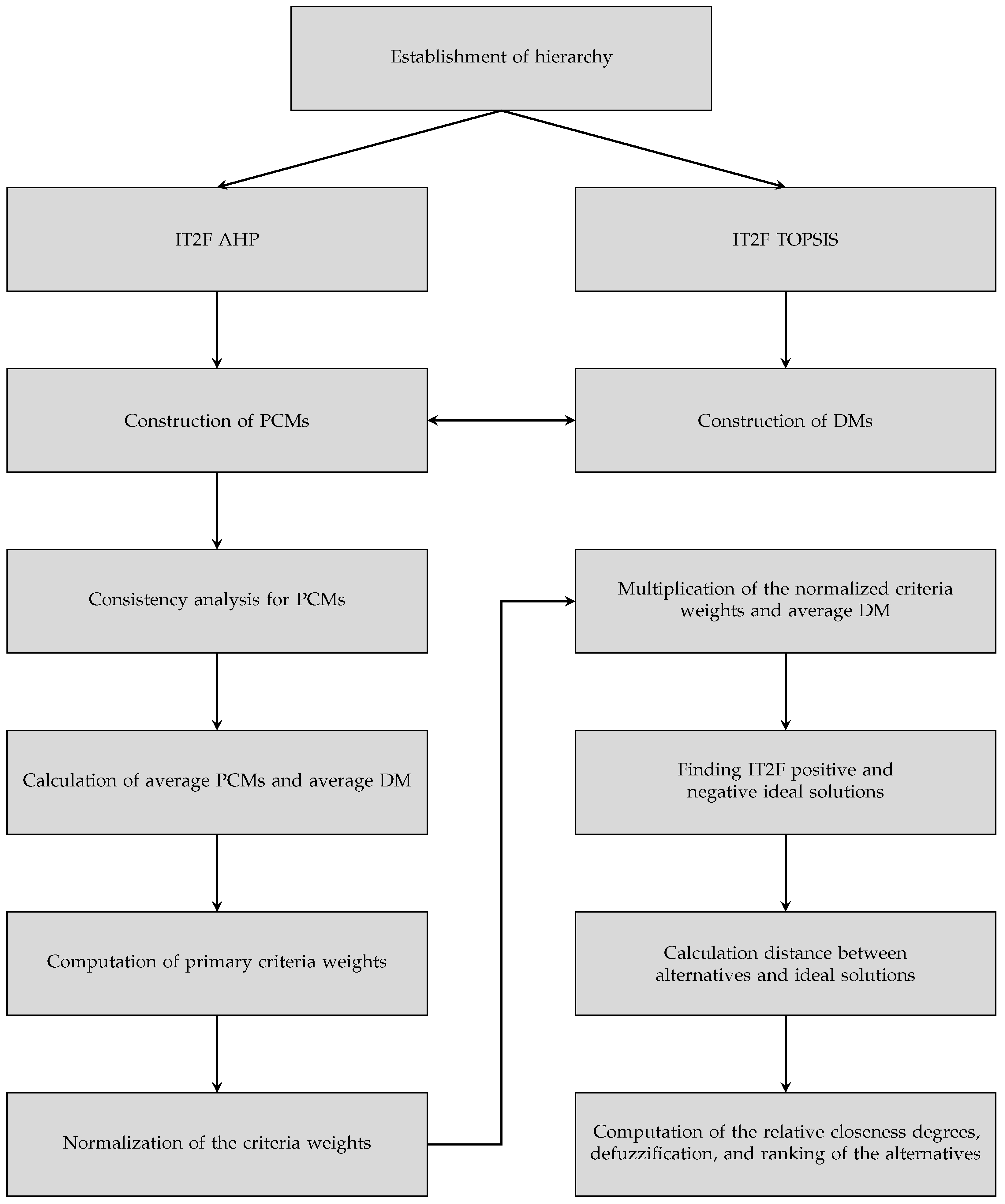
The theoretical procedure described above is summarized in Figure 2.
3. Application
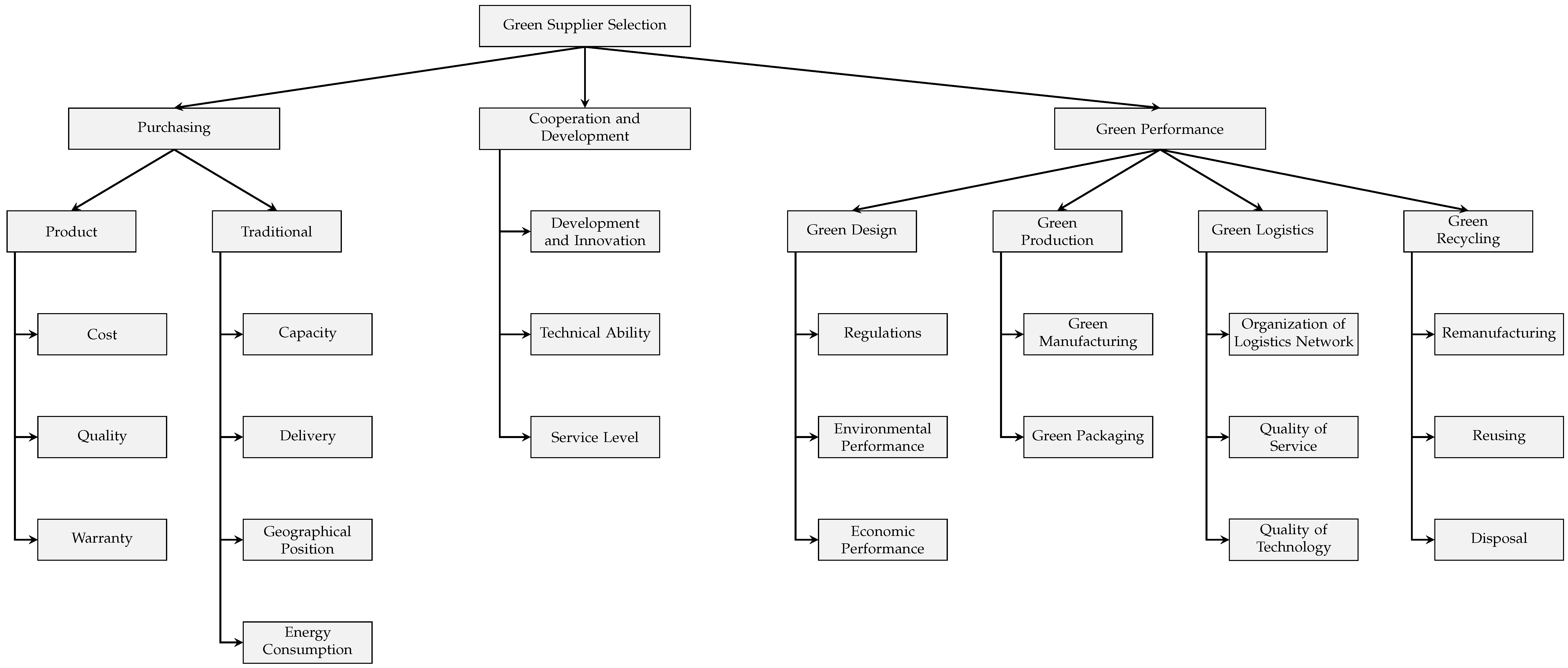
In this study, the GSS problem for the automotive industry will be discussed as an application. Twenty-one criteria shown in Table 1 have been derived from an extensive literature survey; these sub-sub-criteria have been merged into three main criteria and nine sub-criteria. Thus, a multi-level hierarchy has been built for the application to be comprehensive. There is a main criterion signifying “green” and numerous sub-criteria underneath it in the hierarchy. The established hierarchy is depicted in Figure 3. All criteria except “Cost” and “Energy Consumption” have been considered benefit-type criteria. Five alternatives, identified by the letters F to K, include firms operating within the automotive sector for the supplier and will be ranked via the hybrid methodology. The identities of the alternatives will not be disclosed in order to preserve the company’s and suppliers’ privacy. A committee comprising three professionals with different perspectives and over 15 years of professional experience within the industry in Türkiye has been formed to assess the criteria and score the alternatives. In addition, Table 2 provides comprehensive information on the committee.
As described in Section 2.2, first, weights of the criteria will be computed using the AHP process, and then, by aggregating the weights with the alternative scorings, the TOPSIS technique will be employed to produce the optimality rankings of the alternatives. Initially, experts with different perspectives will conduct pairwise comparisons to evaluate weight vectors for criteria at each level. Subsequently, the experts’ evaluations will be utilized to create DMs for each candidate supplier, focusing on the criteria at the lowest level. Proficient decision-makers are required to obtain the PCMs for the AHP method and DMs for the TOPSIS methodology. The MATLAB (version R2021a) package program has been used for all computations in this application.
Step 1:
PCMs have been constructed following the viewpoints of each expert by comparing the criteria in the same sections to each other in pairs. Again, the score of the alternatives under each criterion and DM has been established as a product of each expert’s analysis. While linguistic variables from Table 3 have been utilized to create PCMs, linguistic variables using Table 4 have been employed to generate DMs [39,55]. Due to the high number of criteria in the hierarchy, there are numerous matrices; for the sake of maintaining the readability of the article, matrices and calculations until the normalized weights have been included in Appendix A.
Step 2:
The PCMs that will be used to calculate criteria weights have been defuzzified. The matrices, which consist of crisp equivalents of IT2F elements, have all been confirmed to be consistent.
Step 3:
Step 4:
Step 5:
Normalized criteria weights for criteria at the bottom of the hierarchical structure have been provided via Table 5. Hence, the steps of the AHP technique have been finalized.
Step 6:
The acquired weighted decision matrix, using the final weights of the criteria, is given in Table A22.
Step 7:
Regarding the weighted DM, positive and negative ideal solutions have been acquired and provided via Table 6.
Step 8:
IT2F distances for both types of ideal solutions have been computed, and the obtained results have been presented in Table 7.
Step 9:
The calculated relative closeness degrees for alternatives are given in Table 8. Then, IT2F values have been defuzzified for the eventual classification. The results obtained and the ideal ordering of the alternatives are shown in Table 9. Moreover, the table includes the outcomes obtained from the IT2F AHP-TOPSIS approach for comparison purposes.
The scores from IT2F AHP-TOPSIS and FAHP-FTOPSIS techniques have been normalized to make the comparison more meaningful. As demonstrated by the result table, significant differences exist between the values produced using IT2FNs, and the superiority of the alternatives is evident. However, the data obtained utilizing fuzzy numbers have been conveniently close to each other, so it is impossible to discuss the definitive and indisputable superiority of alternatives over each other. As a natural outcome, the results of the FAHP-FTOPSIS method are untrustworthy and inadequate for making the final decision. Therefore, the IT2F AHP-TOPSIS approach validates that it has been a practical, easily interpretable, and reliable decision-making instrument.
Discussion with Sensitivity Analysis
In addition to the comparison with FAHP-FTOPSIS made at the end of the considered problem, the sensitivity analysis has also been included to assess the robustness of the findings to variations in subjective inputs. For this purpose, the fluctuations of the alternatives in the overall rankings when the importance valuations have been modified and monitored. By that, the criteria weights have been traded amongst each other mutually. Hence, nine additional circumstances have been formed in addition to the initial case. When developing the types of situations, attention has been paid to switching between criteria with dissimilar importance. The following are the scenarios that have been created:
- Scenario I: Weight alteration between “Product Quality” and “Capacity”,
- Scenario II: Weight alteration between “Technical Ability” and “Quality of Service”,
- Scenario III: Weight alteration between “Development and Innovation” and “Geographical Position”,
- Scenario IV: Weight alteration between “Cost” and “Regulations”,
- Scenario V: Weight alteration between “Environmental Performance” and “Delivery”,
- Scenario VI: Weight alteration between “Product Quality” and “Quality of Technology”,
- Scenario VII: Weight alteration between “Technical Ability” and “Disposal”,
- Scenario VIII: Weight alteration between “Development and Innovation” and “Capacity”,
- Scenario IX: Weight alteration between “Cost” and “Quality of Service”.
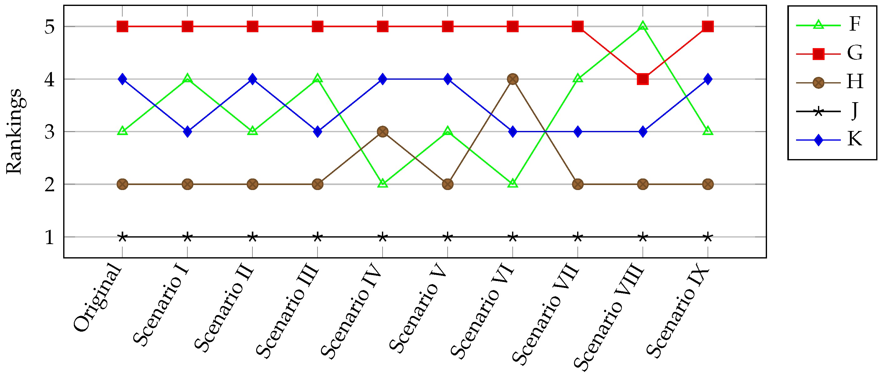
Revised rankings and scores for the various alternatives have been assessed for each redesigned scenario. The obtained data have been shown graphically in Figure 4 and have been listed in Table 10. In light of these findings, Alternative J has been insensitive to weight fluctuations and outperforms the other alternatives regardless of the relevance of the criterion. This points out that Alternative J is almost the best choice, even with the other weightings given to the criteria. Similarly, Alternative G ranks last in 9 out of 10 instances. It did, however, qualify in fourth place on one occasion. Regarding this, it implies that Alternative G has been almost insensitive to the importance levels of the criteria and trails other alternatives in expert assessments. From this point of view, it can be said that Alternative G is not preferable regarding different evaluations for the importance weightings of criteria. On the other hand, it is clear that the rating and positions of Alternatives F, H, and K are quite sensitive to shifts in criteria weights. Alternative H has been generally in the second position, whereas Alternative K remains third or fourth. Alternative F has been the most responsive to the importance assigned to the criterion and varied from second to last. In this case, expert opinions are effective for these three alternative evaluations and rankings. These three may outperform one another under various assessments with different expertise judgments.
4. Conclusions
This study emphasizes the importance of carefully analyzing the GSS process to improve environmental sustainability in supplier selection. It shows the need to define and utilize appropriate criteria and evaluation techniques. Selecting the correct green supplier allows companies to reduce their environmental footprint and gain a competitive advantage at the same time. A hybrid solution method has been proposed by presenting a comprehensive evaluation model that balances both ecological factors and commercial requirements. This model, which incorporates multi-sub-criteria and group decision-making, can guide companies in selecting green suppliers that meet their environmental sustainability goals.
This research utilizes an AHP-TOPSIS hybrid process based on the IT2FN framework to address a noteworthy problem type “GSS” in making a choice or decision-making in the context of ambivalence or unpredictability. A comprehensive hierarchy has been managed by applying the AHP algorithm to successfully determine the importance levels of the criteria with the opinions of a group of experts with different perspectives. While working with such a realistically detailed structure, it has shown the great importance of addressing the evaluation of experts with a framework capable of reflecting the mathematical reality, such as the IT2FNs. After the weightings of the criteria have been completed, to assess the quality of the alternatives successfully, a well-designed TOPSIS methodology that has the ability to maintain the IT2F fabric of the hybridized algorithm has been chosen. As a result, the scores of the alternatives have been obtained, and the best alternative could have easily emerged.
The data collected from the IT2FN variation and the sensitivity analysis have been used to illustrate the process’s validity. The comparison with FAHP-FTOPSIS and IT2F AHP-TOPSIS has revealed that the data gathered with the fuzzy numbers could not yield a clear outcome, while there has been a straightforward ordering in the procedure outlined with the IT2FN structure in this research. Furthermore, changes in the overall rankings of the alternatives were observed when the weights determined using the AHP framework were adjusted in the sensitivity analysis. Consequently, the findings have highlighted that the best evaluation of importance weights could significantly impact the designation of the ideal solution. From best to worst, the preferred ordering as the solution for the given case in this research is Alternative J, Alternative H, Alternative F, Alternative K, and Alternative G. Conclusively, it has been observed that the solution obtained for the thoroughly investigated GSS model is valid and can serve sustainable purposes.
The effectiveness of the proposed methodology in negotiating complicated hierarchical structures inherent in industry-specific contexts is demonstrated by its application in a real-world situation from the automotive industry. For future studies, thanks to the flexibility of the proposed hybrid methodology, any industrial GSS problem based on real data can be solved using the technique. Exploring an alternative MCDM technique to address the complex hierarchy presented in the study could be a potential research area.
Funding
This research received no external funding.
Institutional Review Board Statement
Not applicable.
Informed Consent Statement
Not applicable.
Data Availability Statement
Data are contained within the article.
Conflicts of Interest
The author declares no conflicts of interest.
Appendix A

Table A1.
Average pairwise comparison matrix for main criteria.
| Purchasing | Cooperation and Development | Green Performance | |
|---|---|---|---|
| Purchasing | ((1, 1, 1, 1; 1, 1), (1, 1, 1, 1; 1, 1)) | ((0.6934, 0.7631, 0.9086, 1; 1, 1), (0.7084, 0.7815, 0.891, 0.9811; 0.8, 0.8)) | ((0.5378, 0.6057, 0.8255, 1.0874; 1, 1), (0.5503, 0.6259, 0.7872, 1.0137; 0.8, 0.8)) |
| Cooperation and Development | ((1, 1.1006, 1.3104, 1.4422; 1, 1), (1.0192, 1.1224, 1.2796, 1.4116; 0.8, 0.8)) | ((1, 1, 1, 1; 1, 1), (1, 1, 1, 1; 1, 1)) | ((1.1856, 1.3867, 1.8171, 2.0801; 1, 1), (1.2274, 1.4357, 1.767, 2.0256; 0.8, 0.8)) |
| Green Performance | ((0.9196, 1.2114, 1.651, 1.8594; 1, 1), (0.9865, 1.2703, 1.5977, 1.8171; 0.8, 0.8)) | ((0.4807, 0.5503, 0.7211, 0.8434; 1, 1), (0.4937, 0.5659, 0.6965, 0.8148; 0.8, 0.8)) | ((1, 1, 1, 1; 1, 1), (1, 1, 1, 1; 1, 1)) |
Table A2.
Average pairwise comparison matrix for sub-criteria under Purchasing criterion.
| Product | Traditional | |
|---|---|---|
| Product | ((1, 1, 1, 1; 1, 1), (1, 1, 1, 1; 1, 1)) | ((1.71, 2.0801, 3.1748, 4.3267; 1, 1), (1.7793, 2.1627, 3.024, 4.0111; 0.8, 0.8)) |
| Traditional | ((0.2311, 0.315, 0.4807, 0.5848; 1, 1), (0.2493, 0.3307, 0.4624, 0.562; 0.8, 0.8)) | ((1, 1, 1, 1; 1, 1), (1, 1, 1, 1; 1, 1)) |
Table A3.
Average pairwise comparison matrix for sub-criteria under Cooperation and Development criterion.
Table A3.
Average pairwise comparison matrix for sub-criteria under Cooperation and Development criterion.
| Development and Innovation | Technical Ability | Service Level | |
|---|---|---|---|
| Development and Innovation | ((1, 1, 1, 1; 1, 1), (1, 1, 1, 1; 1, 1)) | ((0.8434, 1, 1.4422, 1.9129; 1, 1), (0.8736, 1.0339, 1.3814, 1.7828; 0.8, 0.8)) | ((4.2172, 5.2415, 7.2685, 8.2768; 1, 1), (4.423, 5.4452, 7.0665, 8.0753; 0.8, 0.8)) |
| Technical Ability | ((0.5228, 0.6934, 1, 1.1856; 1, 1), (0.5609, 0.7239, 0.9672, 1.1447; 0.8, 0.8)) | ((1, 1, 1, 1; 1, 1), (1, 1, 1, 1; 1, 1)) | ((2.7589, 4, 6, 6.8041; 1, 1), (3.0238, 4.2315, 5.7885, 6.6476; 0.8, 0.8)) |
| Service Level | ((0.4297, 0.5, 0.6934, 0.8434; 1, 1), (0.4429, 0.5156, 0.6691, 0.8087; 0.8, 0.8)) | ((0.147, 0.1667, 0.25, 0.3625; 1, 1), (0.1504, 0.1728, 0.2363, 0.3307; 0.8, 0.8)) | ((1, 1, 1, 1; 1, 1), (1, 1, 1, 1; 1, 1)) |
Table A4.
Average pairwise comparison matrix for sub-criteria under Green Performance criterion.
| Green Design | Green Production | Green Logistics | Green Recycling | |
|---|---|---|---|---|
| Green Design | ((1, 1, 1, 1; 1, 1), (1, 1, 1, 1; 1, 1)) | ((0.5848, 0.7937, 1.2599, 1.71; 1, 1), (0.63, 0.8335, 1.1998, 1.5874; 0.8, 0.8)) | ((1.4422, 2.5198, 4.5789, 5.5934; 1, 1), (1.6641, 2.7292, 4.3752, 5.3909; 0.8, 0.8)) | ((0.6934, 0.7937, 1, 1.1187; 1, 1), (0.7138, 0.8136, 0.978, 1.0935; 0.8, 0.8)) |
| Green Production | ((0.5848, 0.7937, 1.2599, 1.71; 1, 1), (0.63, 0.8335, 1.1998, 1.5874; 0.8, 0.8)) | ((1, 1, 1, 1; 1, 1), (1, 1, 1, 1; 1, 1)) | ((2.0801, 2.5198, 3.3019, 3.6593; 1, 1), (2.1715, 2.6032, 3.2281, 3.5893; 0.8, 0.8)) | ((0.4807, 0.7937, 1.3867, 1.71; 1, 1), (0.547, 0.8529, 1.3255, 1.6425; 0.8, 0.8)) |
| Green Logistics | ((0.1788, 0.2184, 0.3969, 0.6934; 1, 1), (0.1855, 0.2286, 0.3664, 0.6009; 0.8, 0.8)) | ((0.2733, 0.3029, 0.3969, 0.4807; 1, 1), (0.2786, 0.3098, 0.3841, 0.4605; 0.8, 0.8)) | ((1, 1, 1, 1; 1, 1), (1, 1, 1, 1; 1, 1)) | ((0.2811, 0.3816, 0.63, 0.8939; 1, 1), (0.3029, 0.4037, 0.595, 0.8221; 0.8, 0.8)) |
| Green Recycling | ((0.8939, 1, 1.2599, 1.4422; 1, 1), (0.9145, 1.0225, 1.2292, 1.401; 0.8, 0.8)) | ((0.5848, 0.7211, 1.2599, 2.0801; 1, 1), (0.6088, 0.7544, 1.1724, 1.8283; 0.8, 0.8)) | ((1.1187, 1.5874, 2.6207, 3.5569; 1, 1), (1.2164, 1.6807, 2.4771, 3.3019; 0.8, 0.8)) | ((1, 1, 1, 1; 1, 1), (1, 1, 1, 1; 1, 1)) |
Table A5.
Average pairwise comparison matrix for sub-criteria under Product sub-criterion.
| Cost | Quality | Warranty | |
|---|---|---|---|
| Cost | ((1, 1, 1, 1; 1, 1), (1, 1, 1, 1; 1, 1)) | ((0.4409, 0.5503, 0.9086, 1.3264; 1, 1), (0.4611, 0.5755, 0.8562, 1.2098; 0.8, 0.8)) | ((1.9129, 2.5198, 3.3019, 3.5569; 1, 1), (2.052, 2.6227, 3.2217, 3.5088; 0.8, 0.8)) |
| Quality | ((0.7539, 1.1006, 1.8171, 2.268; 1, 1), (0.8266, 1.1679, 1.7378, 2.1687; 0.8, 0.8)) | ((1, 1, 1, 1; 1, 1), (1, 1, 1, 1; 1, 1)) | ((2.924, 4.1602, 6.3496, 7.3986; 1, 1), (3.1895, 4.3894, 6.1375, 7.1901; 0.8, 0.8)) |
| Warranty | ((0.2811, 0.3029, 0.3969, 0.5228; 1, 1), (0.285, 0.3104, 0.3813, 0.4873; 0.8, 0.8)) | ((0.1352, 0.1575, 0.2404, 0.342; 1, 1), (0.1391, 0.1629, 0.2278, 0.3135; 0.8, 0.8)) | ((1, 1, 1, 1; 1, 1), (1, 1, 1, 1; 1, 1)) |
Table A6.
Average pairwise comparison matrix for sub-criteria under Traditional sub-criterion.
| Capacity | Delivery | Geographical Position | Energy Consumption | |
|---|---|---|---|---|
| Capacity | ((1, 1, 1, 1; 1, 1), (1, 1, 1, 1; 1, 1)) | ((0.4807, 0.5, 0.5503, 0.5848; 1, 1), (0.4844, 0.5042, 0.5443, 0.5772; 0.8, 0.8)) | ((0.6934, 0.7937, 1, 1.1187; 1, 1), (0.7138, 0.8136, 0.978, 1.0935; 0.8, 0.8)) | ((0.2811, 0.3816, 0.63, 0.8939; 1, 1), (0.3029, 0.4037, 0.595, 0.8221; 0.8, 0.8)) |
| Delivery | ((1.71, 1.8171, 2, 2.0801; 1, 1), (1.7325, 1.8371, 1.9832, 2.0646; 0.8, 0.8)) | ((1, 1, 1, 1; 1, 1), (1, 1, 1, 1; 1, 1)) | ((1.4422, 1.5874, 1.8171, 1.9129; 1, 1), (1.4736, 1.6134, 1.7967, 1.8945; 0.8, 0.8)) | ((0.6934, 0.9615, 1.4422, 1.71; 1, 1), (0.7528, 1.0164, 1.3904, 1.655; 0.8, 0.8)) |
| Geographical Position | ((0.8939, 1, 1.2599, 1.4422; 1, 1), (0.9145, 1.0225, 1.2292, 1.401; 0.8, 0.8)) | ((0.5228, 0.5503, 0.63, 0.6934; 1, 1), (0.5278, 0.5566, 0.6198, 0.6786; 0.8, 0.8)) | ((1, 1, 1, 1; 1, 1), (1, 1, 1, 1; 1, 1)) | ((0.4055, 0.4807, 0.7211, 1; 1, 1), (0.42, 0.5008, 0.6851, 0.9233; 0.8, 0.8)) |
| Energy Consumption | ((1.1187, 1.5874, 2.6207, 3.5569; 1, 1), (1.2164, 1.6807, 2.4771, 3.3019; 0.8, 0.8)) | ((0.5848, 0.6934, 1.04, 1.4422; 1, 1), (0.6042, 0.7192, 0.9839, 1.3283; 0.8, 0.8)) | ((1, 1.3867, 2.0801, 2.4662; 1, 1), (1.0831, 1.4597, 1.9968, 2.3811; 0.8, 0.8)) | ((1, 1, 1, 1; 1, 1), (1, 1, 1, 1; 1, 1)) |
Table A7.
Average pairwise comparison matrix for sub-criteria under Green Design sub-criterion.
| Regulations | Environmental Performance | Economic Performance | |
|---|---|---|---|
| Regulations | ((1, 1, 1, 1; 1, 1), (1, 1, 1, 1; 1, 1)) | ((0.1352, 0.1514, 0.2184, 0.3057; 1, 1), (0.138, 0.1565, 0.2076, 0.2813; 0.8, 0.8)) | ((0.2733, 0.3816, 0.63, 0.8221; 1, 1), (0.2961, 0.4029, 0.5995, 0.7768; 0.8, 0.8)) |
| Environmental Performance | ((3.2711, 4.5789, 6.6039, 7.3986; 1, 1), (3.555, 4.8181, 6.3893, 7.2442; 0.8, 0.8)) | ((1, 1, 1, 1; 1, 1), (1, 1, 1, 1; 1, 1)) | ((1.1187, 1.5874, 2.6207, 3.5569; 1, 1), (1.2164, 1.6807, 2.4771, 3.3019; 0.8, 0.8)) |
| Economic Performance | ((1.2164, 1.5874, 2.6207, 3.6593; 1, 1), (1.2873, 1.6682, 2.4821, 3.3776; 0.8, 0.8)) | ((0.2811, 0.3816, 0.63, 0.8939; 1, 1), (0.3029, 0.4037, 0.595, 0.8221; 0.8, 0.8)) | ((1, 1, 1, 1; 1, 1), (1, 1, 1, 1; 1, 1)) |
Table A8.
Average pairwise comparison matrix for sub-criteria under Green Production sub-criterion.
| Green Manufacturing | Green Packaging | |
|---|---|---|
| Green Manufacturing | ((1, 1, 1, 1; 1, 1), (1, 1, 1, 1; 1, 1)) | ((1.71, 2.2894, 3.1748, 3.5569; 1, 1), (1.841, 2.3893, 3.0948, 3.4826; 0.8, 0.8)) |
| Green Packaging | ((0.2811, 0.315, 0.4368, 0.5848; 1, 1), (0.2871, 0.3231, 0.4185, 0.5432; 0.8, 0.8)) | ((1, 1, 1, 1; 1, 1), (1, 1, 1, 1; 1, 1)) |
Table A9.
Average pairwise comparison matrix for sub-criteria under Green Logistics sub-criterion.
| Organization of Logistics Network | Quality of Service | Quality of Technology | |
|---|---|---|---|
| Organization of Logistics Network | ((1, 1, 1, 1; 1, 1), (1, 1, 1, 1; 1, 1)) | ((1.0874, 1.3867, 2.0801, 2.5372; 1, 1), (1.1462, 1.4489, 28, 2.4357; 0.8, 0.8)) | ((1, 1.2114, 1.651, 1.9129; 1, 1), (1.044, 1.2609, 1.6008, 1.8588; 0.8, 0.8)) |
| Quality of Service | ((0.3941, 0.4807, 0.7211, 0.9196; 1, 1), (0.4106, 0.4998, 0.6902, 0.8724; 0.8, 0.8)) | ((1, 1, 1, 1; 1, 1), (1, 1, 1, 1; 1, 1)) | ((0.5848, 0.63, 0.7937, 1; 1, 1), (0.5928, 0.6408, 0.7689, 0.941; 0.8, 0.8)) |
| Quality of Technology | ((0.5228, 0.6057, 0.8255, 1; 1, 1), (0.538, 0.6247, 0.7931, 0.9579; 0.8, 0.8)) | ((1, 1.2599, 1.5874, 1.71; 1, 1), (1.0627, 1.3006, 1.5605, 1.6869; 0.8, 0.8)) | ((1, 1, 1, 1; 1, 1), (1, 1, 1, 1; 1, 1)) |
Table A10.
Average pairwise comparison matrix for sub-criteria under Green Recycling sub-criterion.
| Remanufacturing | Reusing | Disposal | |
|---|---|---|---|
| Remanufacturing | ((1, 1, 1, 1; 1, 1), (1, 1, 1, 1; 1, 1)) | ((0.5228, 0.5503, 0.63, 0.6934; 1, 1), (0.5278, 0.5566, 0.6198, 0.6786; 0.8, 0.8)) | ((1.4422, 1.8171, 2.8845, 3.9791; 1, 1), (1.5135, 1.8994, 2.7397, 3.6808; 0.8, 0.8)) |
| Reusing | ((1.4422, 1.5874, 1.8171, 1.9129; 1, 1), (1.4736, 1.6134, 1.7967, 1.8945; 0.8, 0.8)) | ((1, 1, 1, 1; 1, 1), (1, 1, 1, 1; 1, 1)) | ((1.9129, 2.2894, 3.3019, 4.3267; 1, 1), (1.9832, 2.374, 3.1481, 4.0412; 0.8, 0.8)) |
| Disposal | ((0.2513, 0.3467, 0.5503, 0.6934; 1, 1), (0.2717, 0.365, 0.5265, 0.6607; 0.8, 0.8)) | ((0.2311, 0.3029, 0.4368, 0.5228; 1, 1), (0.2474, 0.3176, 0.4212, 0.5042; 0.8, 0.8)) | ((1, 1, 1, 1; 1, 1), (1, 1, 1, 1; 1, 1)) |
Table A11.
Average decision matrix for alternatives.
| Criteria | Alternatives | Average of the Rating |
|---|---|---|
| Cost | Alternative F | ((8.3333, 9.5, 9.6667, 10; 1, 1), (9, 9.5, 9.6667, 9.8333; 0.9, 0.9)) |
| Alternative G | ((1.3333, 3, 3.5, 5; 1, 1), (2.1667, 3, 3.5, 4; 0.9, 0.9)) | |
| Alternative H | ((3.6667, 5.5, 6, 7.3333; 1, 1), (4.6667, 5.5, 6, 6.5; 0.9, 0.9)) | |
| Alternative J | ((3.6667, 5.6667, 6.1667, 7.6667; 1, 1), (4.6667, 5.6667, 6.1667, 6.6667; 0.9, 0.9)) | |
| Alternative K | ((5.6667, 7.5, 8, 9.3333; 1, 1), (6.6667, 7.5, 8, 8.5; 0.9, 0.9)) | |
| Product Quality | Alternative F | ((7, 8.5, 8.8333, 9.6667; 1, 1), (7.8333, 8.5, 8.8333, 9.1667; 0.9, 0.9)) |
| Alternative G | ((0.6667, 2.3333, 2.8333, 4.3333; 1, 1), (1.5, 2.3333, 2.8333, 3.3333; 0.9, 0.9)) | |
| Alternative H | ((5.6667, 7.5, 8, 9.3333; 1, 1), (6.6667, 7.5, 8, 8.5; 0.9, 0.9)) | |
| Alternative J | ((5.6667, 7.5, 8, 9.3333; 1, 1), (6.6667, 7.5, 8, 8.5; 0.9, 0.9)) | |
| Alternative K | ((7, 8.5, 8.8333, 9.6667; 1, 1), (7.8333, 8.5, 8.8333, 9.1667; 0.9, 0.9)) | |
| Warranty | Alternative F | ((7, 8.5, 8.8333, 9.6667; 1, 1), (7.8333, 8.5, 8.8333, 9.1667; 0.9, 0.9)) |
| Alternative G | ((2.3333, 4.3333, 4.8333, 6.3333; 1, 1), (3.3333, 4.3333, 4.8333, 5.3333; 0.9, 0.9)) | |
| Alternative H | ((3.6667, 5.6667, 6.1667, 7.6667; 1, 1), (4.6667, 5.6667, 6.1667, 6.6667; 0.9, 0.9)) | |
| Alternative J | ((4.3333, 6.1667, 6.6667, 8; 1, 1), (5.3333, 6.1667, 6.6667, 7.1667; 0.9, 0.9)) | |
| Alternative K | ((4.3333, 6.1667, 6.6667, 8; 1, 1), (5.3333, 6.1667, 6.6667, 7.1667; 0.9, 0.9)) | |
| Capacity | Alternative F | ((1.3333, 2.6667, 3, 4.3333; 1, 1), (2, 2.6667, 3, 3.5; 0.9, 0.9)) |
| Alternative G | ((9, 10, 10, 10; 1, 1), (9.5, 10, 10, 10; 0.9, 0.9)) | |
| Alternative H | ((5, 6.8333, 7.3333, 8.6667; 1, 1), (6, 6.8333, 7.3333, 7.8333; 0.9, 0.9)) | |
| Alternative J | ((6.3333, 8, 8.5, 9.6667; 1, 1), (7.3333, 8, 8.5, 9; 0.9, 0.9)) | |
| Alternative K | ((6.3333, 7.8333, 8.1667, 9; 1, 1), (7.1667, 7.8333, 8.1667, 8.5; 0.9, 0.9)) | |
| Delivery | Alternative F | ((1.3333, 3, 3.5, 5; 1, 1), (2.1667, 3, 3.5, 4; 0.9, 0.9)) |
| Alternative G | ((8.3333, 9.5, 9.6667, 10; 1, 1), (9, 9.5, 9.6667, 9.8333; 0.9, 0.9)) | |
| Alternative H | ((6.3333, 8, 8.5, 9.6667; 1, 1), (7.3333, 8, 8.5, 9; 0.9, 0.9)) | |
| Alternative J | ((5, 6.8333, 7.3333, 8.6667; 1, 1), (6, 6.8333, 7.3333, 7.8333; 0.9, 0.9)) | |
| Alternative K | ((6.3333, 8, 8.3333, 9.3333; 1, 1), (7.1667, 8, 8.3333, 8.6667; 0.9, 0.9)) | |
| Geographical Position | Alternative F | ((2.3333, 4.3333, 4.8333, 6.3333; 1, 1), (3.3333, 4.3333, 4.8333, 5.3333; 0.9, 0.9)) |
| Alternative G | ((8.3333, 9.5, 9.6667, 10; 1, 1), (9, 9.5, 9.6667, 9.8333; 0.9, 0.9)) | |
| Alternative H | ((3.3333, 5, 5.5, 7; 1, 1), (4.1667, 5, 5.5, 6; 0.9, 0.9)) | |
| Alternative J | ((6.3333, 8, 8.5, 9.6667; 1, 1), (7.3333, 8, 8.5, 9; 0.9, 0.9)) | |
| Alternative K | ((5, 6.6667, 7, 8; 1, 1), (5.8333, 6.6667, 7, 7.3333; 0.9, 0.9)) | |
| Energy Consumption | Alternative F | ((5, 6.6667, 7, 8; 1, 1), (5.8333, 6.6667, 7, 7.3333; 0.9, 0.9)) |
| Alternative G | ((2, 3.6667, 4.1667, 5.6667; 1, 1), (2.8333, 3.6667, 4.1667, 4.6667; 0.9, 0.9)) | |
| Alternative H | ((2.3333, 4.3333, 4.8333, 6.3333; 1, 1), (3.3333, 4.3333, 4.8333, 5.3333; 0.9, 0.9)) | |
| Alternative J | ((1.6667, 3.6667, 4.1667, 5.6667; 1, 1), (2.6667, 3.6667, 4.1667, 4.6667; 0.9, 0.9)) | |
| Alternative K | ((4.3333, 6.3333, 6.8333, 8.3333; 1, 1), (5.3333, 6.3333, 6.8333, 7.3333; 0.9, 0.9)) | |
| Development and Innovation | Alternative F | ((7.6667, 9, 9.3333, 10; 1, 1), (8.5, 9, 9.3333, 9.6667; 0.9, 0.9)) |
| Alternative G | ((3, 5, 5.5, 7; 1, 1), (4, 5, 5.5, 6; 0.9, 0.9)) | |
| Alternative H | ((3, 5, 5.5, 7; 1, 1), (4, 5, 5.5, 6; 0.9, 0.9)) | |
| Alternative J | ((5, 6.8333, 7.3333, 8.6667; 1, 1), (6, 6.8333, 7.3333, 7.8333; 0.9, 0.9)) | |
| Alternative K | ((5.6667, 7.1667, 7.5, 8.3333; 1, 1), (6.5, 7.1667, 7.5, 7.8333; 0.9, 0.9)) | |
| Technical Ability | Alternative F | ((7.6667, 9, 9.3333, 10; 1, 1), (8.5, 9, 9.3333, 9.6667; 0.9, 0.9)) |
| Alternative G | ((2.3333, 4.3333, 4.8333, 6.3333; 1, 1), (3.3333, 4.3333, 4.8333, 5.3333; 0.9, 0.9)) | |
| Alternative H | ((4.3333, 6.3333, 6.8333, 8.3333; 1, 1), (5.3333, 6.3333, 6.8333, 7.3333; 0.9, 0.9)) | |
| Alternative J | ((6.3333, 8, 8.3333, 9.3333; 1, 1), (7.1667, 8, 8.3333, 8.6667; 0.9, 0.9)) | |
| Alternative K | ((5.6667, 7.3333, 7.8333, 9; 1, 1), (6.6667, 7.3333, 7.8333, 8.3333; 0.9, 0.9)) | |
| Service Level | Alternative F | ((6.3333, 7.8333, 8.1667, 9; 1, 1), (7.1667, 7.8333, 8.1667, 8.5; 0.9, 0.9)) |
| Alternative G | ((5, 6.8333, 7.3333, 8.6667; 1, 1), (6, 6.8333, 7.3333, 7.8333; 0.9, 0.9)) | |
| Alternative H | ((5.6667, 7.3333, 7.8333, 9; 1, 1), (6.6667, 7.3333, 7.8333, 8.3333; 0.9, 0.9)) | |
| Alternative J | ((6.3333, 8, 8.5, 9.6667; 1, 1), (7.3333, 8, 8.5, 9; 0.9, 0.9)) | |
| Alternative K | ((5.6667, 7.5, 8, 9.3333; 1, 1), (6.6667, 7.5, 8, 8.5; 0.9, 0.9)) | |
| Regulations | Alternative F | ((7, 8.5, 8.8333, 9.6667; 1, 1), (7.8333, 8.5, 8.8333, 9.1667; 0.9, 0.9)) |
| Alternative G | ((3, 5, 5.5, 7; 1, 1), (4, 5, 5.5, 6; 0.9, 0.9)) | |
| Alternative H | ((7.6667, 9, 9.3333, 10; 1, 1), (8.5, 9, 9.3333, 9.6667; 0.9, 0.9)) | |
| Alternative J | ((7, 8.5, 8.8333, 9.6667; 1, 1), (7.8333, 8.5, 8.8333, 9.1667; 0.9, 0.9)) | |
| Alternative K | ((2.3333, 4.3333, 4.8333, 6.3333; 1, 1), (3.3333, 4.3333, 4.8333, 5.3333; 0.9, 0.9)) | |
| Environmental Performance | Alternative F | ((0.6667, 2.3333, 2.8333, 4.3333; 1, 1), (1.5, 2.3333, 2.8333, 3.3333; 0.9, 0.9)) |
| Alternative G | ((1.6667, 3.6667, 4.1667, 5.6667; 1, 1), (2.6667, 3.6667, 4.1667, 4.6667; 0.9, 0.9)) | |
| Alternative H | ((5.6667, 7.5, 8, 9.3333; 1, 1), (6.6667, 7.5, 8, 8.5; 0.9, 0.9)) | |
| Alternative J | ((8.3333, 9.5, 9.6667, 10; 1, 1), (9, 9.5, 9.6667, 9.8333; 0.9, 0.9)) | |
| Alternative K | ((3, 5, 5.5, 7; 1, 1), (4, 5, 5.5, 6; 0.9, 0.9)) | |
| Economic Performance | Alternative F | ((4, 5.5, 6, 7.3333; 1, 1), (4.8333, 5.5, 6, 6.5; 0.9, 0.9)) |
| Alternative G | ((1.6667, 3.6667, 4.1667, 5.6667; 1, 1), (2.6667, 3.6667, 4.1667, 4.6667; 0.9, 0.9)) | |
| Alternative H | ((5, 6.8333, 7.3333, 8.6667; 1, 1), (6, 6.8333, 7.3333, 7.8333; 0.9, 0.9)) | |
| Alternative J | ((7, 8.5, 8.8333, 9.6667; 1, 1), (7.8333, 8.5, 8.8333, 9.1667; 0.9, 0.9)) | |
| Alternative K | ((0.6667, 2.3333, 2.8333, 4.3333; 1, 1), (1.5, 2.3333, 2.8333, 3.3333; 0.9, 0.9)) | |
| Green Manufacturing | Alternative F | ((5.3333, 6.5, 6.8333, 7.6667; 1, 1), (6, 6.5, 6.8333, 7.1667; 0.9, 0.9)) |
| Alternative G | ((0.3333, 1.6667, 2.1667, 3.6667; 1, 1), (1, 1.6667, 2.1667, 2.6667; 0.9, 0.9)) | |
| Alternative H | ((4.3333, 6.1667, 6.6667, 8; 1, 1), (5.3333, 6.1667, 6.6667, 7.1667; 0.9, 0.9)) | |
| Alternative J | ((6.3333, 7.8333, 8.1667, 9; 1, 1), (7.1667, 7.8333, 8.1667, 8.5; 0.9, 0.9)) | |
| Alternative K | ((0, 0.6667, 1, 2.3333; 1, 1), (0.3333, 0.6667, 1, 1.5; 0.9, 0.9)) | |
| Green Packaging | Alternative F | ((3, 5, 5.5, 7; 1, 1), (4, 5, 5.5, 6; 0.9, 0.9)) |
| Alternative G | ((1.6667, 3.6667, 4.1667, 5.6667; 1, 1), (2.6667, 3.6667, 4.1667, 4.6667; 0.9, 0.9)) | |
| Alternative H | ((4.3333, 6.3333, 6.8333, 8.3333; 1, 1), (5.3333, 6.3333, 6.8333, 7.3333; 0.9, 0.9)) | |
| Alternative J | ((5, 6.8333, 7.3333, 8.6667; 1, 1), (6, 6.8333, 7.3333, 7.8333; 0.9, 0.9)) | |
| Alternative K | ((1.6667, 3.6667, 4.1667, 5.6667; 1, 1), (2.6667, 3.6667, 4.1667, 4.6667; 0.9, 0.9)) | |
| Organization of Logistics Network | Alternative F | ((0.3333, 1.3333, 1.6667, 3; 1, 1), (0.8333, 1.3333, 1.6667, 2.1667; 0.9, 0.9)) |
| Alternative G | ((7, 8.5, 8.8333, 9.6667; 1, 1), (7.8333, 8.5, 8.8333, 9.1667; 0.9, 0.9)) | |
| Alternative H | ((4.3333, 6.1667, 6.6667, 8; 1, 1), (5.3333, 6.1667, 6.6667, 7.1667; 0.9, 0.9)) | |
| Alternative J | ((4.3333, 6.3333, 6.8333, 8.3333; 1, 1), (5.3333, 6.3333, 6.8333, 7.3333; 0.9, 0.9)) | |
| Alternative K | ((7.6667, 9, 9.1667, 9.6667; 1, 1), (8.3333, 9, 9.1667, 9.3333; 0.9, 0.9)) | |
| Quality of Service | Alternative F | ((5.6667, 7.3333, 7.8333, 9; 1, 1), (6.6667, 7.3333, 7.8333, 8.3333; 0.9, 0.9)) |
| Alternative G | ((7, 8.5, 8.8333, 9.6667; 1, 1), (7.8333, 8.5, 8.8333, 9.1667; 0.9, 0.9)) | |
| Alternative H | ((6.3333, 8, 8.5, 9.6667; 1, 1), (7.3333, 8, 8.5, 9; 0.9, 0.9)) | |
| Alternative J | ((6.3333, 8, 8.3333, 9.3333; 1, 1), (7.1667, 8, 8.3333, 8.6667; 0.9, 0.9)) | |
| Alternative K | ((5, 6.6667, 7, 8; 1, 1), (5.8333, 6.6667, 7, 7.3333; 0.9, 0.9)) | |
| Quality of Technology | Alternative F | ((6.3333, 7.6667, 7.8333, 8.3333; 1, 1), (7, 7.6667, 7.8333, 8; 0.9, 0.9)) |
| Alternative G | ((4.3333, 6.1667, 6.6667, 8; 1, 1), (5.3333, 6.1667, 6.6667, 7.1667; 0.9, 0.9)) | |
| Alternative H | ((1.6667, 2.6667, 3, 4.3333; 1, 1), (2.1667, 2.6667, 3, 3.5; 0.9, 0.9)) | |
| Alternative J | ((6.3333, 8, 8.3333, 9.3333; 1, 1), (7.1667, 8, 8.3333, 8.6667; 0.9, 0.9)) | |
| Alternative K | ((6.3333, 8, 8.5, 9.6667; 1, 1), (7.3333, 8, 8.5, 9; 0.9, 0.9)) | |
| Remanufacturing | Alternative F | ((6.3333, 7.6667, 7.8333, 8.3333; 1, 1), (7, 7.6667, 7.8333, 8; 0.9, 0.9)) |
| Alternative G | ((5, 6.8333, 7.3333, 8.6667; 1, 1), (6, 6.8333, 7.3333, 7.8333; 0.9, 0.9)) | |
| Alternative H | ((5.6667, 7.5, 8, 9.3333; 1, 1), (6.6667, 7.5, 8, 8.5; 0.9, 0.9)) | |
| Alternative J | ((3.6667, 5.6667, 6.1667, 7.6667; 1, 1), (4.6667, 5.6667, 6.1667, 6.6667; 0.9, 0.9)) | |
| Alternative K | ((3.6667, 5.6667, 6.1667, 7.6667; 1, 1), (4.6667, 5.6667, 6.1667, 6.6667; 0.9, 0.9)) | |
| Reusing | Alternative F | ((3.6667, 5.6667, 6.1667, 7.6667; 1, 1), (4.6667, 5.6667, 6.1667, 6.6667; 0.9, 0.9)) |
| Alternative G | ((7.6667, 9, 9.3333, 10; 1, 1), (8.5, 9, 9.3333, 9.6667; 0.9, 0.9)) | |
| Alternative H | ((6.3333, 8, 8.5, 9.6667; 1, 1), (7.3333, 8, 8.5, 9; 0.9, 0.9)) | |
| Alternative J | ((5.6667, 7.5, 8, 9.3333; 1, 1), (6.6667, 7.5, 8, 8.5; 0.9, 0.9)) | |
| Alternative K | ((6.3333, 7.8333, 8.1667, 9; 1, 1), (7.1667, 7.8333, 8.1667, 8.5; 0.9, 0.9)) | |
| Disposal | Alternative F | ((3.6667, 5.6667, 6.1667, 7.6667; 1, 1), (4.6667, 5.6667, 6.1667, 6.6667; 0.9, 0.9)) |
| Alternative G | ((6.3333, 8, 8.5, 9.6667; 1, 1), (7.3333, 8, 8.5, 9; 0.9, 0.9)) | |
| Alternative H | ((5, 6.6667, 7, 8; 1, 1), (5.8333, 6.6667, 7, 7.3333; 0.9, 0.9)) | |
| Alternative J | ((2.3333, 4.3333, 4.8333, 6.3333; 1, 1), (3.3333, 4.3333, 4.8333, 5.3333; 0.9, 0.9)) | |
| Alternative K | ((7, 8.5, 8.8333, 9.6667; 1, 1), (7.8333, 8.5, 8.8333, 9.1667; 0.9, 0.9)) |
Table A12.
Local weights of main criteria.
| Purchasing | ((0.1982, 0.234, 0.3247, 0.4049; 1, 1), (0.2054, 0.2434, 0.3111, 0.3847; 0.8, 0.8)) |
| Cooperation and Development | ((0.2914, 0.3485, 0.4772, 0.5678; 1, 1), (0.3029, 0.3621, 0.4595, 0.547; 0.8, 0.8)) |
| Green Performance | ((0.2097, 0.2644, 0.3788, 0.4574; 1, 1), (0.2212, 0.2767, 0.3628, 0.4392; 0.8, 0.8)) |
Table A13.
Local weights of sub-criteria under Purchasing criterion.
| Product | ((0.4597, 0.5827, 0.8894, 1.1631; 1, 1), (0.4846, 0.608, 0.8501, 1.0925; 0.8, 0.8)) |
| Traditional | ((0.169, 0.2267, 0.3461, 0.4276; 1, 1), (0.1814, 0.2377, 0.3324, 0.4089; 0.8, 0.8)) |
Table A14.
Local weights of sub-criteria under Cooperation and Development criterion.
| Development and Innovation | ((0.2941, 0.3807, 0.6115, 0.8221; 1, 1), (0.3111, 0.3994, 0.5811, 0.7681; 0.8, 0.8)) |
| Technical Ability | ((0.2177, 0.3079, 0.5077, 0.6566; 1, 1), (0.2364, 0.3261, 0.4828, 0.621; 0.8, 0.8)) |
| Service Level | ((0.0767, 0.0957, 0.1558, 0.2205; 1, 1), (0.0804, 0.1003, 0.147, 0.2034; 0.8, 0.8)) |
Table A15.
Local weights of sub-criteria under Green Performance criterion.
| Green Design | ((0.1419, 0.2206, 0.4214, 0.6098; 1, 1), (0.1578, 0.2369, 0.395, 0.5604; 0.8, 0.8)) |
| Green Production | ((0.1419, 0.2206, 0.4214, 0.6098; 1, 1), (0.1578, 0.2369, 0.395, 0.5604; 0.8, 0.8)) |
| Green Logistics | ((0.0555, 0.0783, 0.1526, 0.2491; 1, 1), (0.06, 0.0835, 0.1412, 0.2213; 0.8, 0.8)) |
| Green Recycling | ((0.1419, 0.2033, 0.3883, 0.6094; 1, 1), (0.1539, 0.2167, 0.3607, 0.5464; 0.8, 0.8)) |
Table A16.
Local weights of sub-criteria under Product sub-criterion.
| Cost | ((0.1968, 0.2681, 0.4596, 0.6494; 1, 1), (0.211, 0.2835, 0.4327, 0.5988; 0.8, 0.8)) |
| Quality | ((0.2711, 0.3993, 0.72, 0.9913; 1, 1), (0.297, 0.4261, 0.6791, 0.9239; 0.8, 0.8)) |
| Warranty | ((0.07, 0.0872, 0.1456, 0.2181; 1, 1), (0.0733, 0.0914, 0.1366, 0.1977; 0.8, 0.8)) |
Table A17.
Local weights of sub-criteria under Traditional sub-criterion.
| Capacity | ((0.1029, 0.1329, 0.205, 0.2686; 1, 1), (0.1092, 0.1394, 0.1954, 0.2525; 0.8, 0.8)) |
| Delivery | ((0.2127, 0.275, 0.4042, 0.496; 1, 1), (0.226, 0.2878, 0.3887, 0.4745; 0.8, 0.8)) |
| Geographical Position | ((0.1227, 0.1528, 0.2324, 0.3071; 1, 1), (0.1288, 0.1596, 0.2214, 0.2879; 0.8, 0.8)) |
| Energy Consumption | ((0.1673, 0.2368, 0.4123, 0.5792; 1, 1), (0.1813, 0.2518, 0.3869, 0.5347; 0.8, 0.8)) |
Table A18.
Local weights of sub-criteria under Green Design sub-criterion.
| Regulations | ((0.0654, 0.0902, 0.1629, 0.2452; 1, 1), (0.0705, 0.0959, 0.1521, 0.2227; 0.8, 0.8)) |
| Environmental Performance | ((0.3028, 0.4521, 0.816, 1.1559; 1, 1), (0.3332, 0.484, 0.7648, 1.0655; 0.8, 0.8)) |
| Economic Performance | ((0.1374, 0.1975, 0.3729, 0.5769; 1, 1), (0.1494, 0.2113, 0.3469, 0.5198; 0.8, 0.8)) |
Table A19.
Local weights of sub-criteria under Green Production sub-criterion.
| Green Manufacturing | ((0.4933, 0.6194, 0.859, 1.0262; 1, 1), (0.5212, 0.6424, 0.8321, 0.986; 0.8, 0.8)) |
| Green Packaging | ((0.2, 0.2298, 0.3186, 0.4161; 1, 1), (0.2058, 0.2362, 0.306, 0.3894; 0.8, 0.8)) |
Table A20.
Local weights of sub-criteria under Green Logistics sub-criterion.
| Organization of Logistics Network | ((0.2663, 0.3462, 0.5438, 0.6919; 1, 1), (0.282, 0.3641, 0.5191, 0.6575; 0.8, 0.8)) |
| Quality of Service | ((0.1588, 0.1956, 0.2993, 0.3974; 1, 1), (0.1659, 0.2038, 0.2851, 0.3722; 0.8, 0.8)) |
| Quality of Technology | ((0.2086, 0.2662, 0.3945, 0.4887; 1, 1), (0.2205, 0.2779, 0.3781, 0.4664; 0.8, 0.8)) |
Table A21.
Local weights of sub-criteria under Green Recycling sub-criterion.
| Remanufacturing | ((0.2199, 0.2733, 0.4055, 0.5195; 1, 1), (0.2308, 0.2845, 0.3885, 0.4908; 0.8, 0.8)) |
| Reusing | ((0.3389, 0.4202, 0.6039, 0.7492; 1, 1), (0.3556, 0.437, 0.5802, 0.713; 0.8, 0.8)) |
| Disposal | ((0.0936, 0.1289, 0.2066, 0.2641; 1, 1), (0.1011, 0.1362, 0.1971, 0.2508; 0.8, 0.8)) |
Table A22.
Weighted decision matrix for alternatives.
| Criteria | Alternatives | Average of the Rating |
|---|---|---|
| Cost | Alternative F | ((0.1494, 0.3474, 1.2828, 3.0581; 1, 1), (0.189, 0.3985, 1.1061, 2.4745; 0.8, 0.8)) |
| Alternative G | ((0.0239, 0.1097, 0.4645, 1.529; 1, 1), (0.0455, 0.1258, 0.4005, 1.0066; 0.8, 0.8)) | |
| Alternative H | ((0.0657, 0.2011, 0.7962, 2.2426; 1, 1), (0.098, 0.2307, 0.6866, 1.6357; 0.8, 0.8)) | |
| Alternative J | ((0.0657, 0.2072, 0.8184, 2.3445; 1, 1), (0.098, 0.2377, 0.7056, 1.6776; 0.8, 0.8)) | |
| Alternative K | ((0.1016, 0.2742, 1.0617, 2.8542; 1, 1), (0.14, 0.3146, 0.9154, 2.139; 0.8, 0.8)) | |
| Product Quality | Alternative F | ((0.1729, 0.4628, 1.8366, 4.5124; 1, 1), (0.2315, 0.5359, 1.5864, 3.5592; 0.8, 0.8)) |
| Alternative G | ((0.0165, 0.1271, 0.5891, 2.0228; 1, 1), (0.0443, 0.1471, 0.5089, 1.2943; 0.8, 0.8)) | |
| Alternative H | ((0.1399, 0.4084, 1.6634, 4.3568; 1, 1), (0.197, 0.4729, 1.4368, 3.3004; 0.8, 0.8)) | |
| Alternative J | ((0.1399, 0.4084, 1.6634, 4.3568; 1, 1), (0.197, 0.4729, 1.4368, 3.3004; 0.8, 0.8)) | |
| Alternative K | ((0.1729, 0.4628, 1.8366, 4.5124; 1, 1), (0.2315, 0.5359, 1.5864, 3.5592; 0.8, 0.8)) | |
| Warranty | Alternative F | ((0.0447, 0.1011, 0.3714, 0.9929; 1, 1), (0.0571, 0.1149, 0.3192, 0.7616; 0.8, 0.8)) |
| Alternative G | ((0.0149, 0.0515, 0.2032, 0.6505; 1, 1), (0.0243, 0.0586, 0.1747, 0.4431; 0.8, 0.8)) | |
| Alternative H | ((0.0234, 0.0674, 0.2593, 0.7875; 1, 1), (0.034, 0.0766, 0.2228, 0.5539; 0.8, 0.8)) | |
| Alternative J | ((0.0276, 0.0733, 0.2803, 0.8217; 1, 1), (0.0389, 0.0834, 0.2409, 0.5955; 0.8, 0.8)) | |
| Alternative K | ((0.0276, 0.0733, 0.2803, 0.8217; 1, 1), (0.0389, 0.0834, 0.2409, 0.5955; 0.8, 0.8)) | |
| Capacity | Alternative F | ((0.0046, 0.0188, 0.0691, 0.2015; 1, 1), (0.0081, 0.0215, 0.0606, 0.139; 0.8, 0.8)) |
| Alternative G | ((0.031, 0.0705, 0.2304, 0.465; 1, 1), (0.0386, 0.0806, 0.2021, 0.3972; 0.8, 0.8)) | |
| Alternative H | ((0.0172, 0.0482, 0.1689, 0.403; 1, 1), (0.0244, 0.0551, 0.1482, 0.3111; 0.8, 0.8)) | |
| Alternative J | ((0.0218, 0.0564, 0.1958, 0.4495; 1, 1), (0.0298, 0.0645, 0.1718, 0.3574; 0.8, 0.8)) | |
| Alternative K | ((0.0218, 0.0553, 0.1881, 0.4185; 1, 1), (0.0292, 0.0632, 0.165, 0.3376; 0.8, 0.8)) | |
| Delivery | Alternative F | ((0.0095, 0.0438, 0.159, 0.4294; 1, 1), (0.0182, 0.05, 0.1407, 0.2986; 0.8, 0.8)) |
| Alternative G | ((0.0594, 0.1386, 0.4391, 0.8587; 1, 1), (0.0758, 0.1582, 0.3885, 0.734; 0.8, 0.8)) | |
| Alternative H | ((0.0451, 0.1167, 0.3861, 0.8301; 1, 1), (0.0617, 0.1332, 0.3416, 0.6718; 0.8, 0.8)) | |
| Alternative J | ((0.0356, 0.0997, 0.3331, 0.7442; 1, 1), (0.0505, 0.1138, 0.2947, 0.5847; 0.8, 0.8)) | |
| Alternative K | ((0.0451, 0.1167, 0.3785, 0.8015; 1, 1), (0.0603, 0.1332, 0.3349, 0.6469; 0.8, 0.8)) | |
| Geographical Position | Alternative F | ((0.0096, 0.0351, 0.1262, 0.3367; 1, 1), (0.016, 0.04, 0.1107, 0.2416; 0.8, 0.8)) |
| Alternative G | ((0.0342, 0.077, 0.2524, 0.5317; 1, 1), (0.0432, 0.0877, 0.2213, 0.4454; 0.8, 0.8)) | |
| Alternative H | ((0.0137, 0.0405, 0.1436, 0.3722; 1, 1), (0.02, 0.0462, 0.1259, 0.2718; 0.8, 0.8)) | |
| Alternative J | ((0.026, 0.0649, 0.222, 0.514; 1, 1), (0.0352, 0.0739, 0.1946, 0.4076; 0.8, 0.8)) | |
| Alternative K | ((0.0205, 0.0541, 0.1828, 0.4254; 1, 1), (0.028, 0.0616, 0.1603, 0.3322; 0.8, 0.8)) | |
| Energy Consumption | Alternative F | ((0.028, 0.0838, 0.3243, 0.8022; 1, 1), (0.0394, 0.0971, 0.2801, 0.6169; 0.8, 0.8)) |
| Alternative G | ((0.0112, 0.0461, 0.193, 0.5682; 1, 1), (0.0191, 0.0534, 0.1667, 0.3926; 0.8, 0.8)) | |
| Alternative H | ((0.0131, 0.0545, 0.2239, 0.6351; 1, 1), (0.0225, 0.0631, 0.1934, 0.4486; 0.8, 0.8)) | |
| Alternative J | ((0.0093, 0.0461, 0.193, 0.5682; 1, 1), (0.018, 0.0534, 0.1667, 0.3926; 0.8, 0.8)) | |
| Alternative K | ((0.0243, 0.0796, 0.3166, 0.8356; 1, 1), (0.036, 0.0923, 0.2734, 0.6169; 0.8, 0.8)) | |
| Development and Innovation | Alternative F | ((0.657, 1.194, 2.7238, 4.6678; 1, 1), (0.801, 1.3019, 2.4924, 4.0614; 0.8, 0.8)) |
| Alternative G | ((0.2571, 0.6633, 1.6051, 3.2675; 1, 1), (0.3769, 0.7233, 1.4687, 2.5209; 0.8, 0.8)) | |
| Alternative H | ((0.2571, 0.6633, 1.6051, 3.2675; 1, 1), (0.3769, 0.7233, 1.4687, 2.5209; 0.8, 0.8)) | |
| Alternative J | ((0.4285, 0.9065, 2.1401, 4.0455; 1, 1), (0.5654, 0.9885, 1.9583, 3.2911; 0.8, 0.8)) | |
| Alternative K | ((0.4856, 0.9507, 2.1888, 3.8899; 1, 1), (0.6125, 1.0367, 2.0028, 3.2911; 0.8, 0.8)) | |
| Technical Ability | Alternative F | ((0.4863, 0.9657, 2.2615, 3.7282; 1, 1), (0.6087, 1.0628, 2.0708, 3.2838; 0.8, 0.8)) |
| Alternative G | ((0.148, 0.465, 1.1711, 2.3612; 1, 1), (0.2387, 0.5117, 1.0724, 1.8117; 0.8, 0.8)) | |
| Alternative H | ((0.2749, 0.6796, 1.6558, 3.1069; 1, 1), (0.382, 0.7479, 1.5161, 2.4912; 0.8, 0.8)) | |
| Alternative J | ((0.4017, 0.8584, 2.0192, 3.4797; 1, 1), (0.5133, 0.9447, 1.8489, 2.9441; 0.8, 0.8)) | |
| Alternative K | ((0.3594, 0.7869, 1.8981, 3.3554; 1, 1), (0.4774, 0.866, 1.738, 2.8309; 0.8, 0.8)) | |
| Service Level | Alternative F | ((0.1416, 0.2613, 0.6072, 1.127; 1, 1), (0.1745, 0.2845, 0.5518, 0.9458; 0.8, 0.8)) |
| Alternative G | ((0.1118, 0.2279, 0.5452, 1.0853; 1, 1), (0.1461, 0.2481, 0.4955, 0.8716; 0.8, 0.8)) | |
| Alternative H | ((0.1267, 0.2446, 0.5824, 1.127; 1, 1), (0.1623, 0.2663, 0.5293, 0.9273; 0.8, 0.8)) | |
| Alternative J | ((0.1416, 0.2669, 0.632, 1.2105; 1, 1), (0.1785, 0.2905, 0.5743, 1.0014; 0.8, 0.8)) | |
| Alternative K | ((0.1267, 0.2502, 0.5948, 1.1688; 1, 1), (0.1623, 0.2724, 0.5405, 0.9458; 0.8, 0.8)) | |
| Regulations | Alternative F | ((0.0136, 0.0447, 0.2296, 0.6613; 1, 1), (0.0193, 0.0535, 0.1925, 0.5026; 0.8, 0.8)) |
| Alternative G | ((0.0058, 0.0263, 0.143, 0.4788; 1, 1), (0.0098, 0.0314, 0.1199, 0.329; 0.8, 0.8)) | |
| Alternative H | ((0.0149, 0.0474, 0.2426, 0.6841; 1, 1), (0.0209, 0.0566, 0.2034, 0.53; 0.8, 0.8)) | |
| Alternative J | ((0.0136, 0.0447, 0.2296, 0.6613; 1, 1), (0.0193, 0.0535, 0.1925, 0.5026; 0.8, 0.8)) | |
| Alternative K | ((0.0045, 0.0228, 0.1256, 0.4332; 1, 1), (0.0082, 0.0273, 0.1053, 0.2924; 0.8, 0.8)) | |
| Environmental Performance | Alternative F | ((0.006, 0.0615, 0.369, 1.3972; 1, 1), (0.0174, 0.074, 0.3106, 0.8742; 0.8, 0.8)) |
| Alternative G | ((0.015, 0.0967, 0.5427, 1.8271; 1, 1), (0.031, 0.1164, 0.4567, 1.2239; 0.8, 0.8)) | |
| Alternative H | ((0.0511, 0.1977, 1.042, 3.0093; 1, 1), (0.0775, 0.238, 0.8769, 2.2293; 0.8, 0.8)) | |
| Alternative J | ((0.0751, 0.2505, 1.2591, 3.2242; 1, 1), (0.1047, 0.3015, 1.0596, 2.579; 0.8, 0.8)) | |
| Alternative K | ((0.027, 0.1318, 0.7164, 2.257; 1, 1), (0.0465, 0.1587, 0.6029, 1.5736; 0.8, 0.8)) | |
| Economic Performance | Alternative F | ((0.0164, 0.0633, 0.3571, 1.18; 1, 1), (0.0252, 0.0762, 0.2983, 0.8316; 0.8, 0.8)) |
| Alternative G | ((0.0068, 0.0422, 0.248, 0.9118; 1, 1), (0.0139, 0.0508, 0.2072, 0.5971; 0.8, 0.8)) | |
| Alternative H | ((0.0204, 0.0787, 0.4364, 1.3945; 1, 1), (0.0313, 0.0946, 0.3646, 1.0022; 0.8, 0.8)) | |
| Alternative J | ((0.0286, 0.0979, 0.5257, 1.5555; 1, 1), (0.0408, 0.1177, 0.4392, 1.1728; 0.8, 0.8)) | |
| Alternative K | ((0.0027, 0.0269, 0.1686, 0.6973; 1, 1), (0.0078, 0.0323, 0.1409, 0.4265; 0.8, 0.8)) | |
| Green Manufacturing | Alternative F | ((0.0783, 0.2348, 0.9369, 2.1945; 1, 1), (0.1091, 0.2738, 0.8149, 1.7394; 0.8, 0.8)) |
| Alternative G | ((0.0049, 0.0602, 0.2971, 1.0495; 1, 1), (0.0182, 0.0702, 0.2584, 0.6472; 0.8, 0.8)) | |
| Alternative H | ((0.0636, 0.2228, 0.914, 2.2899; 1, 1), (0.097, 0.2597, 0.795, 1.7394; 0.8, 0.8)) | |
| Alternative J | ((0.093, 0.283, 1.1197, 2.5761; 1, 1), (0.1304, 0.3299, 0.9739, 2.063; 0.8, 0.8)) | |
| Alternative K | ((, 0.0241, 0.1371, 0.6679; 1, 1), (0.0061, 0.0281, 0.1193, 0.3641; 0.8, 0.8)) | |
| Green Packaging | Alternative F | ((0.0179, 0.067, 0.2797, 0.8124; 1, 1), (0.0287, 0.0774, 0.2412, 0.5751; 0.8, 0.8)) |
| Alternative G | ((0.0099, 0.0491, 0.2119, 0.6577; 1, 1), (0.0192, 0.0568, 0.1827, 0.4473; 0.8, 0.8)) | |
| Alternative H | ((0.0258, 0.0849, 0.3475, 0.9672; 1, 1), (0.0383, 0.0981, 0.2997, 0.7029; 0.8, 0.8)) | |
| Alternative J | ((0.0298, 0.0916, 0.3729, 1.0059; 1, 1), (0.0431, 0.1058, 0.3216, 0.7508; 0.8, 0.8)) | |
| Alternative K | ((0.0099, 0.0491, 0.2119, 0.6577; 1, 1), (0.0192, 0.0568, 0.1827, 0.4473; 0.8, 0.8)) | |
| Organization of Logistics Network | Alternative F | ((0.001, 0.0096, 0.0524, 0.2365; 1, 1), (0.0031, 0.0112, 0.0443, 0.1385; 0.8, 0.8)) |
| Alternative G | ((0.0217, 0.061, 0.2777, 0.7621; 1, 1), (0.0293, 0.0715, 0.2348, 0.5858; 0.8, 0.8)) | |
| Alternative H | ((0.0134, 0.0442, 0.2096, 0.6307; 1, 1), (0.02, 0.0519, 0.1772, 0.458; 0.8, 0.8)) | |
| Alternative J | ((0.0134, 0.0454, 0.2148, 0.657; 1, 1), (0.02, 0.0533, 0.1817, 0.4687; 0.8, 0.8)) | |
| Alternative K | ((0.0238, 0.0645, 0.2881, 0.7621; 1, 1), (0.0312, 0.0757, 0.2437, 0.5965; 0.8, 0.8)) | |
| Quality of Service | Alternative F | ((0.0105, 0.0297, 0.1355, 0.4076; 1, 1), (0.0147, 0.0345, 0.1144, 0.3014; 0.8, 0.8)) |
| Alternative G | ((0.0129, 0.0344, 0.1528, 0.4377; 1, 1), (0.0172, 0.04, 0.129, 0.3316; 0.8, 0.8)) | |
| Alternative H | ((0.0117, 0.0324, 0.147, 0.4377; 1, 1), (0.0161, 0.0377, 0.1241, 0.3256; 0.8, 0.8)) | |
| Alternative J | ((0.0117, 0.0324, 0.1442, 0.4227; 1, 1), (0.0158, 0.0377, 0.1217, 0.3135; 0.8, 0.8)) | |
| Alternative K | ((0.0092, 0.027, 0.1211, 0.3623; 1, 1), (0.0128, 0.0314, 0.1022, 0.2653; 0.8, 0.8)) | |
| Quality of Technology | Alternative F | ((0.001, 0.0096, 0.0524, 0.2365; 1, 1), (0.0031, 0.0112, 0.0443, 0.1385; 0.8, 0.8)) |
| Alternative G | ((0.0217, 0.061, 0.2777, 0.7621; 1, 1), (0.0293, 0.0715, 0.2348, 0.5858; 0.8, 0.8)) | |
| Alternative H | ((0.0134, 0.0442, 0.2096, 0.6307; 1, 1), (0.02, 0.0519, 0.1772, 0.458; 0.8, 0.8)) | |
| Alternative J | ((0.0134, 0.0454, 0.2148, 0.657; 1, 1), (0.02, 0.0533, 0.1817, 0.4687; 0.8, 0.8)) | |
| Alternative K | ((0.0238, 0.0645, 0.2881, 0.7621; 1, 1), (0.0312, 0.0757, 0.2437, 0.5965; 0.8, 0.8)) | |
| Remanufacturing | Alternative F | ((0.0105, 0.0297, 0.1355, 0.4076; 1, 1), (0.0147, 0.0345, 0.1144, 0.3014; 0.8, 0.8)) |
| Alternative G | ((0.0129, 0.0344, 0.1528, 0.4377; 1, 1), (0.0172, 0.04, 0.129, 0.3316; 0.8, 0.8)) | |
| Alternative H | ((0.0117, 0.0324, 0.147, 0.4377; 1, 1), (0.0161, 0.0377, 0.1241, 0.3256; 0.8, 0.8)) | |
| Alternative J | ((0.0117, 0.0324, 0.1442, 0.4227; 1, 1), (0.0158, 0.0377, 0.1217, 0.3135; 0.8, 0.8)) | |
| Alternative K | ((0.0092, 0.027, 0.1211, 0.3623; 1, 1), (0.0128, 0.0314, 0.1022, 0.2653; 0.8, 0.8)) | |
| Reusing | Alternative F | ((0.0154, 0.0423, 0.1786, 0.464; 1, 1), (0.0205, 0.0492, 0.1517, 0.3627; 0.8, 0.8)) |
| Alternative G | ((0.0105, 0.034, 0.152, 0.4455; 1, 1), (0.0156, 0.0396, 0.1291, 0.3249; 0.8, 0.8)) | |
| Alternative H | ((0.0041, 0.0147, 0.0684, 0.2413; 1, 1), (0.0063, 0.0171, 0.0581, 0.1587; 0.8, 0.8)) | |
| Alternative J | ((0.0154, 0.0441, 0.19, 0.5197; 1, 1), (0.021, 0.0514, 0.1614, 0.3929; 0.8, 0.8)) | |
| Alternative K | ((0.0154, 0.0441, 0.1938, 0.5383; 1, 1), (0.0215, 0.0514, 0.1646, 0.408; 0.8, 0.8)) | |
| Disposal | Alternative F | ((0.0414, 0.1126, 0.4672, 1.2067; 1, 1), (0.055, 0.1308, 0.3983, 0.9425; 0.8, 0.8)) |
| Alternative G | ((0.0327, 0.1004, 0.4374, 1.2549; 1, 1), (0.0471, 0.1166, 0.3728, 0.9228; 0.8, 0.8)) | |
| Alternative H | ((0.0371, 0.1102, 0.4772, 1.3515; 1, 1), (0.0524, 0.128, 0.4067, 1.0014; 0.8, 0.8)) | |
| Alternative J | ((0.024, 0.0832, 0.3678, 1.1101; 1, 1), (0.0367, 0.0967, 0.3135, 0.7854; 0.8, 0.8)) | |
| Alternative K | ((0.024, 0.0832, 0.3678, 1.1101; 1, 1), (0.0367, 0.0967, 0.3135, 0.7854; 0.8, 0.8)) |
References
- Noci, G. Designing ‘green’ vendor rating systems for the assessment of a supplier’s environmental performance. Eur. J. Purch. Supply Manag. 1997, 3, 103–114. [Google Scholar] [CrossRef]
- Govindan, K.; Rajendran, S.; Sarkis, J.; Murugesan, P. Multi criteria decision making approaches for green supplier evaluation and selection: A literature review. J. Clean. Prod. 2015, 98, 66–83. [Google Scholar] [CrossRef]
- Tronnebati, I.; El Yadari, M.; Jawab, F. A Review of Green Supplier Evaluation and Selection Issues Using MCDM, MP and AI Models. Sustainability 2022, 14, 16714. [Google Scholar] [CrossRef]
- Dweiri, F.; Kumar, S.; Khan, S.A.; Jain, V. Designing an integrated AHP based decision support system for supplier selection in automotive industry. Expert Syst. Appl. 2016, 62, 273–283. [Google Scholar] [CrossRef]
- Barrios, M.A.O.; De Felice, F.; Negrete, K.P.; Romero, B.A.; Arenas, A.Y.; Petrillo, A. An AHP-TOPSIS integrated model for selecting the most appropriate tomography equipment. Int. J. Inf. Technol. Decis. Mak. 2016, 15, 861–885. [Google Scholar] [CrossRef]
- Yu, Q.; Hou, F. An approach for green supplier selection in the automobile manufacturing industry. Kybernetes 2016, 45, 571–588. [Google Scholar] [CrossRef]
- Zhu, S.; Li, D.; Feng, H.; Gu, T.; Zhu, J. AHP-TOPSIS-based evaluation of the relative performance of multiple neighborhood renewal projects: A case study in Nanjing, China. Sustainability 2019, 11, 4545. [Google Scholar] [CrossRef]
- Navarro, N.; Valverde, P.D.F.; Quesada, H.J.; Madrigal-Sánchez, J. A supplier selection model for the wood fiber supply industry. BioResources 2020, 15, 1959–1977. [Google Scholar] [CrossRef]
- James, A.T.; Vaidya, D.; Sodawala, M.; Verma, S. Selection of bus chassis for large fleet operators in India: An AHP-TOPSIS approach. Expert Syst. Appl. 2021, 186, 115760. [Google Scholar] [CrossRef]
- Gitelman, L.D.; Kozhevnikov, M.V. New approaches to the concept of energy transition in the times of energy crisis. Sustainability 2023, 15, 5167. [Google Scholar] [CrossRef]
- Zeng, F.; Li, J. Study on comprehensive evaluation and countermeasures of natural gas safety in EU. Energy Strategy Rev. 2023, 49, 101167. [Google Scholar] [CrossRef]
- Kannan, D.; de Sousa Jabbour, A.B.L.; Jabbour, C.J.C. Selecting green suppliers based on GSCM practices: Using fuzzy TOPSIS applied to a Brazilian electronics company. Eur. J. Oper. Res. 2014, 233, 432–447. [Google Scholar] [CrossRef]
- Keshavarz Ghorabaee, M.; Amiri, M.; Zavadskas, E.K.; Antucheviciene, J. Supplier evaluation and selection in fuzzy environments: A review of MADM approaches. Econ. Res.-Ekon. Istraživanja 2017, 30, 1073–1118. [Google Scholar] [CrossRef]
- Wang Chen, H.M.; Chou, S.-Y.; Luu, Q.D.; Yu, T.H.-K. A fuzzy MCDM approach for green supplier selection from the economic and environmental aspects. Math. Probl. Eng. 2016, 2016, 8097386. [Google Scholar] [CrossRef]
- Samanlioglu, F.; Taskaya, Y.E.; Gulen, U.C.; Cokcan, O. A fuzzy AHP-TOPSIS-based group decision-making approach to IT personnel selection. Int. J. Fuzzy Syst. 2018, 20, 1576–1591. [Google Scholar] [CrossRef]
- Jain, V.; Sangaiah, A.K.; Sakhuja, S.; Thoduka, N.; Aggarwal, R. Supplier selection using fuzzy AHP and TOPSIS: A case study in the Indian automotive industry. Neural Comput. Appl. 2018, 29, 555–564. [Google Scholar] [CrossRef]
- Venkatesh, V.; Zhang, A.; Deakins, E.; Luthra, S.; Mangla, S. A fuzzy AHP-TOPSIS approach to supply partner selection in continuous aid humanitarian supply chains. Ann. Oper. Res. 2019, 283, 1517–1550. [Google Scholar] [CrossRef]
- Pehlivan, N.Y.; Ünal, Y.; Kahraman, C. Player Selection for a National Football Team using Fuzzy AHP and Fuzzy TOPSIS. J. Mult.-Valued Log. Soft Comput. 2019, 32, 369. [Google Scholar]
- Li, J.; Fang, H.; Song, W. Sustainable supplier selection based on SSCM practices: A rough cloud TOPSIS approach. J. Clean. Prod. 2019, 222, 606–621. [Google Scholar] [CrossRef]
- Nasrollahi, H.; Ahmadi, F.; Ebadollahi, M.; Nobar, S.N.; Amidpour, M. The greenhouse technology in different climate conditions: A comprehensive energy-saving analysis. Sustain. Energy Technol. Assess. 2021, 47, 101455. [Google Scholar] [CrossRef]
- Ekmekcioğlu, Ö.; Koc, K.; Özger, M. Stakeholder perceptions in flood risk assessment: A hybrid fuzzy AHP-TOPSIS approach for Istanbul, Turkey. Int. J. Disaster Risk Reduct. 2021, 60, 102327. [Google Scholar] [CrossRef]
- Yildizbasi, A.; Arioz, Y. Green supplier selection in new era for sustainability: A novel method for integrating big data analytics and a hybrid fuzzy multi-criteria decision making. Soft Comput. 2022, 26, 253–270. [Google Scholar] [CrossRef]
- Bhattacherjee, A.; Kukreja, V.; Aggarwal, A. Stakeholders’ perspective towards employability: A hybrid fuzzy AHP-TOPSIS Approach. Educ. Inf. Technol. 2023, 29, 2157–2181. [Google Scholar] [CrossRef]
- Bozanic, D.; Tešić, D.; Komazec, N.; Marinković, D.; Puška, A. Interval fuzzy AHP method in risk assessment. Rep. Mech. Eng. 2023, 4, 131–140. [Google Scholar] [CrossRef]
- Ghazvinian, A.; Feng, B.; Feng, J.; Talebzadeh, H.; Dzikuć, M. Lean, Agile, Resilient, Green, and Sustainable (LARGS) Supplier Selection Using Multi-Criteria Structural Equation Modeling under Fuzzy Environments. Sustainability 2024, 16, 1594. [Google Scholar] [CrossRef]
- Erdoğan, M.; Kaya, I. A combined fuzzy approach to determine the best region for a nuclear power plant in Turkey. Appl. Soft Comput. 2016, 39, 84–93. [Google Scholar] [CrossRef]
- Mousakhani, S.; Nazari-Shirkouhi, S.; Bozorgi-Amiri, A. A novel interval type-2 fuzzy evaluation model based group decision analysis for green supplier selection problems: A case study of battery industry. J. Clean. Prod. 2017, 168, 205–218. [Google Scholar] [CrossRef]
- Celik, E.; Akyuz, E. An interval type-2 fuzzy AHP and TOPSIS methods for decision-making problems in maritime transportation engineering: The case of ship loader. Ocean Eng. 2018, 155, 371–381. [Google Scholar] [CrossRef]
- Alegoz, M.; Yapicioglu, H. Supplier selection and order allocation decisions under quantity discount and fast service options. Sustain. Prod. Consum. 2019, 18, 179–189. [Google Scholar] [CrossRef]
- Wu, Y.; Xu, C.; Zhang, B.; Tao, Y.; Li, X.; Chu, H.; Liu, F. Sustainability performance assessment of wind power coupling hydrogen storage projects using a hybrid evaluation technique based on interval type-2 fuzzy set. Energy 2019, 179, 1176–1190. [Google Scholar] [CrossRef]
- Mathew, M.; Chakrabortty, R.K.; Ryan, M.J. Selection of an optimal maintenance strategy under uncertain conditions: An interval type-2 fuzzy AHP-TOPSIS method. IEEE Trans. Eng. Manag. 2020, 69, 1121–1134. [Google Scholar] [CrossRef]
- Kiracı, K.; Akan, E. Aircraft selection by applying AHP and TOPSIS in interval type-2 fuzzy sets. J. Air Transp. Manag. 2020, 89, 101924. [Google Scholar] [CrossRef] [PubMed]
- Yılmaz, H.; Kabak, Ö. Prioritizing distribution centers in humanitarian logistics using type-2 fuzzy MCDM approach. J. Enterp. Inf. Manag. 2020, 33, 1199–1232. [Google Scholar] [CrossRef]
- Meniz, B.; Tiryaki, F. Mobile app evaluation application with AHP method based on interval type-2 fuzzy sets. Aip Conf. Proc. 2021, 2325, 20044. [Google Scholar]
- Ecer, F. Multi-criteria decision making for green supplier selection using interval type-2 fuzzy AHP: A case study of a home appliance manufacturer. Oper. Res. 2022, 22, 199–233. [Google Scholar] [CrossRef]
- Sari, I.U.; Tüysüz, N. COVID-19 Risk Assessment of Occupations Using Interval Type 2 Fuzzy Z-AHP & Topsis Methodology. J. Mult.-Valued Log. Soft Comput. 2022, 38, 575. [Google Scholar]
- Chen, S.M.; Lee, L.W. Fuzzy multiple attributes group decision-making based on the interval type-2 TOPSIS method. Expert Syst. Appl. 2010, 37, 2790–2798. [Google Scholar] [CrossRef]
- Meniz, B. An advanced TOPSIS method with new fuzzy metric based on interval type-2 fuzzy sets. Expert Syst. Appl. 2021, 186, 115770. [Google Scholar] [CrossRef]
- Kahraman, C.; Öztayşi, B.; Sarı, İ.U.; Turanoğlu, E. Fuzzy analytic hierarchy process with interval type-2 fuzzy sets. Knowl.-Based Syst. 2014, 59, 48–57. [Google Scholar] [CrossRef]
- Meniz, B.; Akin Bas, S.; Ahlatcioglu Ozkok, B.; Tiryaki, F. Multilevel AHP approach with interval type-2 fuzzy sets to portfolio selection problem. J. Intell. Fuzzy Syst. 2021, 40, 8819–8829. [Google Scholar] [CrossRef]
- Büyüközkan, G.; Çifçi, G. A novel fuzzy multi-criteria decision framework for sustainable supplier selection with incomplete information. Comput. Ind. 2011, 62, 164–174. [Google Scholar] [CrossRef]
- Awasthi, A.; Kannan, G. Green supplier development program selection using NGT and VIKOR under fuzzy environment. Comput. Ind. Eng. 2016, 91, 100–108. [Google Scholar] [CrossRef]
- Banaeian, N.; Mobli, H.; Nielsen, I.E.; Omid, M. Criteria definition and approaches in green supplier selection–a case study for raw material and packaging of food industry. Prod. Manuf. Res. 2015, 3, 149–168. [Google Scholar] [CrossRef]
- Torabzadeh Khorasani, S. Green supplier evaluation by using the integrated fuzzy AHP model and fuzzy copras. Process Integr. Optim. Sustain. 2018, 2, 17–25. [Google Scholar] [CrossRef]
- Wang, C.N.; Nguyen, T.L.; Dang, T.T. Two-Stage Fuzzy MCDM for Green Supplier Selection in Steel Industry. Intell. Autom. Soft Comput. 2022, 33, 1245–1260. [Google Scholar] [CrossRef]
- Chung, C.C.; Chao, L.C.; Lou, S.J. The establishment of a green supplier selection and guidance mechanism with the ANP and IPA. Sustainability 2016, 8, 259. [Google Scholar] [CrossRef]
- Jasch, C. Environmental performance evaluation and indicators. J. Clean. Prod. 2000, 8, 79–88. [Google Scholar] [CrossRef]
- Henri, J.F.; Journeault, M. Environmental performance indicators: An empirical study of Canadian manufacturing firms. J. Environ. Manag. 2008, 87, 165–176. [Google Scholar] [CrossRef]
- Wang, K.Q.; Liu, H.C.; Liu, L.; Huang, J. Green supplier evaluation and selection using cloud model theory and the QUALIFLEX method. Sustainability 2017, 9, 688. [Google Scholar] [CrossRef]
- Lee, A.H.; Kang, H.Y.; Hsu, C.F.; Hung, H.C. A green supplier selection model for high-tech industry. Expert Syst. Appl. 2009, 36, 7917–7927. [Google Scholar] [CrossRef]
- Mathiyazhagan, K.; Sudhakar, S.; Bhalotia, A. Modeling the criteria for selection of suppliers towards green aspect: A case in Indian automobile industry. Opsearch 2018, 55, 65–84. [Google Scholar] [CrossRef]
- Mohammadi, H.; Farahani, F.V.; Noroozi, M.; Lashgari, A. Green supplier selection by developing a new group decision-making method under type 2 fuzzy uncertainty. Int. J. Adv. Manuf. Technol. 2017, 93, 1443–1462. [Google Scholar] [CrossRef]
- Diabat, A.; Khodaverdi, R.; Olfat, L. An exploration of green supply chain practices and performances in an automotive industry. Int. J. Adv. Manuf. Technol. 2013, 68, 949–961. [Google Scholar] [CrossRef]
- Sahu, A.K.; Datta, S.; Mahapatra, S. Evaluation and selection of suppliers considering green perspectives: Comparative analysis on application of FMLMCDM and fuzzy-TOPSIS. Benchmarking Int. J. 2016, 23, 1579–1604. [Google Scholar] [CrossRef]
- Ghorabaee, M.K.; Amiri, M.; Zavadskas, E.K.; Turskis, Z.; Antucheviciene, J. A new multi-criteria model based on interval type-2 fuzzy sets and EDAS method for supplier evaluation and order allocation with environmental considerations. Comput. Ind. Eng. 2017, 112, 156–174. [Google Scholar] [CrossRef]
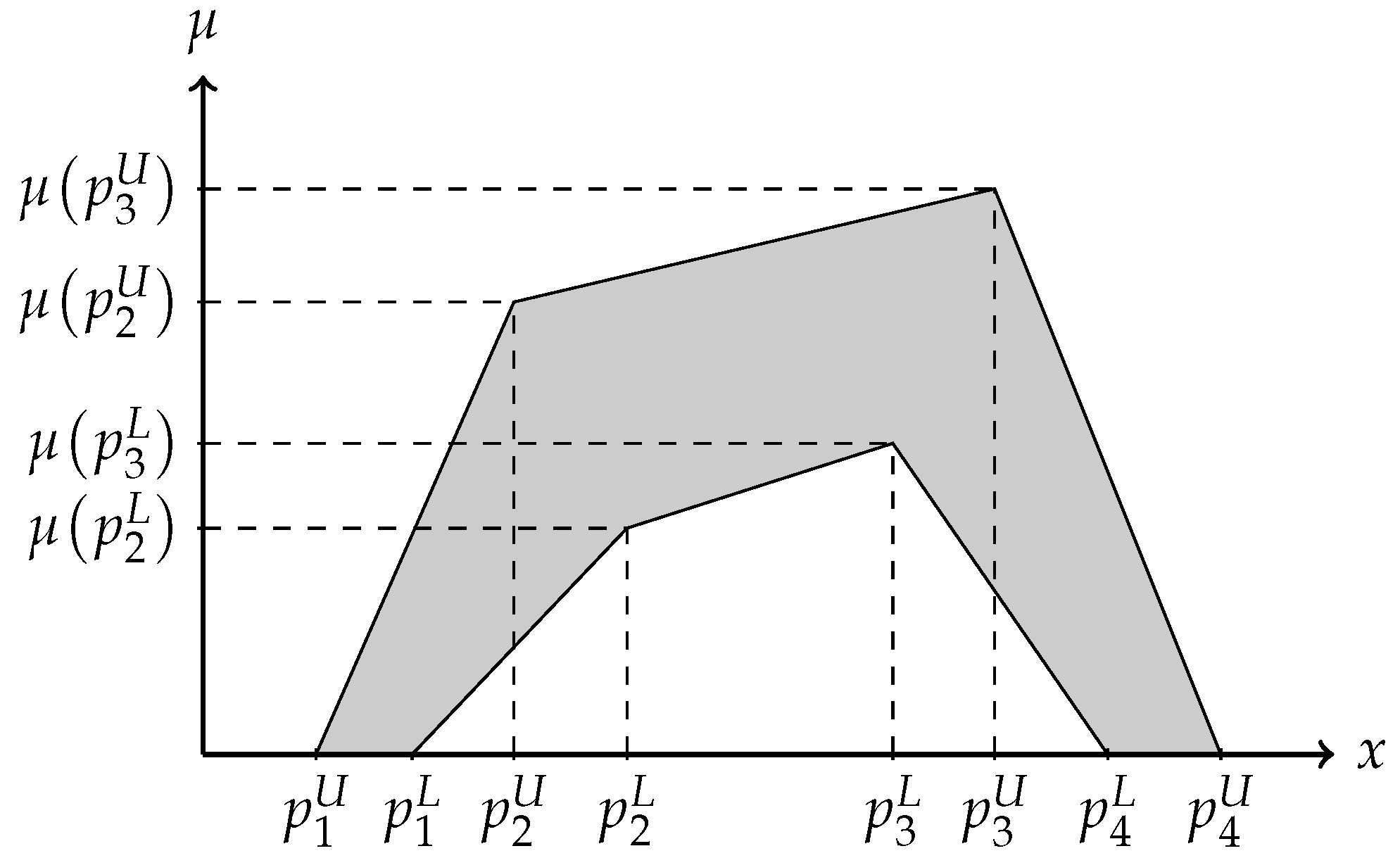
Figure 1.
Interval type-2 fuzzy number.

Figure 2.
Formal description of the methodology.

Figure 3.
Hierarchy proposed for the GSS problem.

Figure 4.
Optimal decision alterations with various weightings.

Table 1.
Description of GSS criteria, sub-criteria and sub-sub-criteria.
| Criteria (1st-Level) | Sub-Criteria (2nd-Level) | Sub-Sub-Criteria (3rd-Level) | Description | References |
|---|---|---|---|---|
| Purchasing () | Product () | Cost () | The cost of material, manufacturing, and inventory | [6,22,41,42] |
| Quality () | The procurable quality attributes by the supplier | [6,22,41,43] | ||
| Warranty () | The duration of the supplier’s warranty on the product that has been delivered | [44,45] | ||
| Traditional () | Capacity () | The product capacity of supplier | [46] | |
| Delivery () | The frequency of product delivery by the supplier on a certain date | [43,45,46] | ||
| Geographical Position () | The location of supplier affecting delivery time, transportation and production costs | [6] | ||
| Energy Consumption () | The total energy consumed by supplier during its operation | [42,44,47,48] | ||
| Cooperation and Development () | Development and Innovation () | The supplier’s ability to innovate in integrating economic and environmental performance | [6] | |
| Technical Ability () | The internal technical capability and the capacity to adapt to future changes in the firm’s requirements | [6,44] | ||
| Service Level () | The supplier ability of flexibility and information | [6] | ||
| Green Performance () | Green Design () | Regulations () | The ability of supplier to comply with government regulations | [49] |
| Environmental Performance () | The assessment of how to reduce its environmental impact taking into account aspects | [12,49] | ||
| such as energy efficiency, resource conservation, and waste reduction | ||||
| Economic Performance () | The assessment of the cost-effectiveness and financial viability of implementing sustainable practices | [49] | ||
| taking into account factors such as initial investment, operational costs, and long-term savings | ||||
| Green Production () | Green Manufacturing () | The environmentally friendly production | [35,49] | |
| Green Packaging () | The recyclable product packaging design | [35,49,50,51] | ||
| Green Logistics () | Organization of Logistics Network () | The logistics network organization’s scope | [49] | |
| Quality of Service () | The internal service quality for logistics | [41,49,52] | ||
| Quality of Technology () | The internal technology quality for logistics | [49] | ||
| Green Recycling () | Remanufacturing () | The efficient retrieval of recycled materials for the initial material production | [35,51,53,54] | |
| Reusing () | The reusability aspects for products | [22,35,51,53,54] | ||
| Disposal () | The elimination of scrap, excess, wastes, etc., without the intention to retrieve | [49,54] |
Table 2.
Detailed committee information.
| Expert | Title | Education | Experience (Years) |
|---|---|---|---|
| 1 | Procurement Manager | Masters in Finance | 19 |
| 2 | Supply Chain Manager | Masters in Industrial Engineering | 16 |
| 3 | Procurement Specialist | Masters in Business Administration | 15 |
Table 3.
IT2F scale for pairwise comparisons.
| Abbreviation | Corresponding IT2FN |
|---|---|
| AS | |
| E | |
| FS | |
| SS | |
| VS |
AS: Absolutely Strong, E: Equal, FS: Fairly Strong. SS: Slightly Strong, VS: Very Strong.
Table 4.
IT2F scale for rating alternatives.
| Abbreviation | Corresponding IT2FN |
|---|---|
| F | |
| G | |
| MG | |
| MP | |
| P | |
| VG | |
| VP |
F: Fair, G: Good, MG: Medium Good, MP: Medium Poor. P: Poor, VG: Very Good, VP: Very Poor.
Table 5.
Normalized weights for the lowest level criteria.
| Criteria | IT2F Weight |
|---|---|
| Cost | ((0.0179, 0.0366, 0.1327, 0.3058; 1, 1), (0.021, 0.0419, 0.1144, 0.2516; 0.8, 0.8)) |
| Product Quality | ((0.0247, 0.0545, 0.2079, 0.4668; 1, 1), (0.0296, 0.0631, 0.1796, 0.3883; 0.8, 0.8)) |
| Warranty | ((0.0064, 0.0119, 0.042, 0.1027; 1, 1), (0.0073, 0.0135, 0.0361, 0.0831; 0.8, 0.8)) |
| Capacity | ((0.0034, 0.0071, 0.023, 0.0465; 1, 1), (0.0041, 0.0081, 0.0202, 0.0397; 0.8, 0.8)) |
| Delivery | ((0.0071, 0.0146, 0.0454, 0.0859; 1, 1), (0.0084, 0.0167, 0.0402, 0.0746; 0.8, 0.8)) |
| Geographical Position | ((0.0041, 0.0081, 0.0261, 0.0532; 1, 1), (0.0048, 0.0092, 0.0229, 0.0453; 0.8, 0.8)) |
| Energy Consumption | ((0.0056, 0.0126, 0.0463, 0.1003; 1, 1), (0.0068, 0.0146, 0.04, 0.0841 ; 0.8, 0.8)) |
| Development and Innovation | ((0.0857, 0.1327, 0.2918, 0.4668; 1, 1), (0.0942, 0.1447, 0.267, 0.4201; 0.8, 0.8)) |
| Technical Ability | ((0.0634, 0.1073, 0.2423, 0.3728; 1, 1), (0.0716, 0.1181, 0.2219, 0.3397; 0.8, 0.8)) |
| Service Level | ((0.0224, 0.0334, 0.0743, 0.1252; 1, 1), (0.0243, 0.0363, 0.0676, 0.1113; 0.8, 0.8)) |
| Regulations | ((0.0019, 0.0053, 0.026, 0.0684; 1, 1), (0.0025, 0.0063, 0.0218, 0.0548; 0.8, 0.8)) |
| Environmental Performance | ((0.009, 0.0264, 0.1302, 0.3224; 1, 1), (0.0116, 0.0317, 0.1096, 0.2623; 0.8, 0.8)) |
| Economic Performance | ((0.0041, 0.0115, 0.0595, 0.1609; 1, 1), (0.0052, 0.0139, 0.0497, 0.1279; 0.8, 0.8)) |
| Green Manufacturing | ((0.0147, 0.0361, 0.1371, 0.2862; 1, 1), (0.0182, 0.0421, 0.1193, 0.2427; 0.8, 0.8)) |
| Green Packaging | ((0.006, 0.0134, 0.0509, 0.1161; 1, 1), (0.0072, 0.0155, 0.0439, 0.0959; 0.8, 0.8)) |
| Organization of Logistics Network | ((0.0031, 0.0072, 0.0314, 0.0788; 1, 1), (0.0037, 0.0084, 0.0266, 0.0639; 0.8, 0.8)) |
| Quality of Service | ((0.0018, 0.0041, 0.0173, 0.0453; 1, 1), (0.0022, 0.0047, 0.0146, 0.0362; 0.8, 0.8)) |
| Quality of Technology | ((0.0024, 0.0055, 0.0228, 0.0557; 1, 1), (0.0029, 0.0064, 0.0194, 0.0453; 0.8, 0.8)) |
| Remanufacturing | ((0.0065, 0.0147, 0.0596, 0.1448; 1, 1), (0.0079, 0.0171, 0.0508, 0.1178; 0.8, 0.8)) |
| Reusing | ((0.0101, 0.0226, 0.0888, 0.2088; 1, 1), (0.0121, 0.0262, 0.0759, 0.1711; 0.8, 0.8)) |
| Disposal | ((0.0028, 0.0069, 0.0304, 0.0736; 1, 1), (0.0034, 0.0082, 0.0258, 0.0602; 0.8, 0.8)) |
Table 6.
Positive and negative ideal solutions.
| Criteria | Positive Ideal Solution | Negative Ideal Solution |
|---|---|---|
| Cost | ((0.0239, 0.1097, 0.4645, 1.529; 1, 1), (0.0455, 0.1258, 0.4005, 1.0066; 0.8, 0.8)) | ((0.1494, 0.3474, 1.2828, 3.0581; 1, 1), (0.189, 0.3985, 1.1061, 2.4745; 0.8, 0.8)) |
| Product Quality | ((0.1729, 0.4628, 1.8366, 4.5124; 1, 1), (0.2315, 0.5359, 1.5864, 3.5592; 0.8, 0.8)) | ((0.0165, 0.1271, 0.5891, 2.0228; 1, 1), (0.0443, 0.1471, 0.5089, 1.2943; 0.8, 0.8)) |
| Warranty | ((0.0447, 0.1011, 0.3714, 0.9929; 1, 1), (0.0571, 0.1149, 0.3192, 0.7616; 0.8, 0.8)) | ((0.0149, 0.0515, 0.2032, 0.6505; 1, 1), (0.0243, 0.0586, 0.1747, 0.4431; 0.8, 0.8)) |
| Capacity | ((0.031, 0.0705, 0.2304, 0.465; 1, 1), (0.0386, 0.0806, 0.2021, 0.3972; 0.8, 0.8)) | ((0.0046, 0.0188, 0.0691, 0.2015; 1, 1), (0.0081, 0.0215, 0.0606, 0.139; 0.8, 0.8)) |
| Delivery | ((0.0594, 0.1386, 0.4391, 0.8587; 1, 1), (0.0758, 0.1582, 0.3885, 0.734; 0.8, 0.8)) | ((0.0095, 0.0438, 0.159, 0.4294; 1, 1), (0.0182, 0.05, 0.1407, 0.2986; 0.8, 0.8)) |
| Geographical Position | ((0.0342, 0.077, 0.2524, 0.5317; 1, 1), (0.0432, 0.0877, 0.2213, 0.4454; 0.8, 0.8)) | ((0.0096, 0.0351, 0.1262, 0.3367; 1, 1), (0.016, 0.04, 0.1107, 0.2416; 0.8, 0.8)) |
| Energy Consumption | ((0.0093, 0.0461, 0.193, 0.5682; 1, 1), (0.018, 0.0534, 0.1667, 0.3926; 0.8, 0.8)) | ((0.028, 0.0838, 0.3243, 0.8356; 1, 1), (0.0394, 0.0971, 0.2801, 0.6169; 0.8, 0.8)) |
| Development and Innovation | ((0.657, 1.194, 2.7238, 4.6678; 1, 1), (0.801, 1.3019, 2.4924, 4.0614; 0.8, 0.8)) | ((0.2571, 0.6633, 1.6051, 3.2675; 1, 1), (0.3769, 0.7233, 1.4687, 2.5209; 0.8, 0.8)) |
| Technical Ability | ((0.4863, 0.9657, 2.2615, 3.7282; 1, 1), (0.6087, 1.0628, 2.0708, 3.2838; 0.8, 0.8)) | ((0.148, 0.465, 1.1711, 2.3612; 1, 1), (0.2387, 0.5117, 1.0724, 1.8117; 0.8, 0.8)) |
| Service Level | ((0.1416, 0.2669, 0.632, 1.2105; 1, 1), (0.1785, 0.2905, 0.5743, 1.0014; 0.8, 0.8)) | ((0.1118, 0.2279, 0.5452, 1.0853; 1, 1), (0.1461, 0.2481, 0.4955, 0.8716; 0.8, 0.8)) |
| Regulations | ((0.0149, 0.0474, 0.2426, 0.6841; 1, 1), (0.0209, 0.0566, 0.2034, 0.53; 0.8, 0.8)) | ((0.0045, 0.0228, 0.1256, 0.4332; 1, 1), (0.0082, 0.0273, 0.1053, 0.2924; 0.8, 0.8)) |
| Environmental Performance | ((0.0751, 0.2505, 1.2591, 3.2242; 1, 1), (0.1047, 0.3015, 1.0596, 2.579; 0.8, 0.8)) | ((0.006, 0.0615, 0.369, 1.3972; 1, 1), (0.0174, 0.074, 0.3106, 0.8742; 0.8, 0.8)) |
| Economic Performance | ((0.0286, 0.0979, 0.5257, 1.5555; 1, 1), (0.0408, 0.1177, 0.4392, 1.1728; 0.8, 0.8)) | ((0.0027, 0.0269, 0.1686, 0.6973; 1, 1), (0.0078, 0.0323, 0.1409, 0.4265; 0.8, 0.8)) |
| Green Manufacturing | ((0.093, 0.283, 1.1197, 2.5761; 1, 1), (0.1304, 0.3299, 0.9739, 2.063; 0.8, 0.8)) | ((, 0.0241, 0.1371, 0.6679; 1, 1), (0.0061, 0.0281, 0.1193, 0.3641; 0.8, 0.8)) |
| Green Packaging | ((0.0298, 0.0916, 0.3729, 1.0059; 1, 1), (0.0431, 0.1058, 0.3216, 0.7508; 0.8, 0.8)) | ((0.0099, 0.0491, 0.2119, 0.6577; 1, 1), (0.0192, 0.0568, 0.1827, 0.4473; 0.8, 0.8)) |
| Organization of Logistics Network | ((0.0238, 0.0645, 0.2881, 0.7621; 1, 1), (0.0312, 0.0757, 0.2437, 0.5965; 0.8, 0.8)) | ((0.001, 0.0096, 0.0524, 0.2365; 1, 1), (0.0031, 0.0112, 0.0443, 0.1385; 0.8, 0.8)) |
| Quality of Service | ((0.0129, 0.0344, 0.1528, 0.4377; 1, 1), (0.0172, 0.04, 0.129, 0.3316; 0.8, 0.8)) | ((0.0092, 0.027, 0.1211, 0.3623; 1, 1), (0.0128, 0.0314, 0.1022, 0.2653; 0.8, 0.8)) |
| Quality of Technology | ((0.0154, 0.0441, 0.1938, 0.5383; 1, 1), (0.0215, 0.0514, 0.1646, 0.408; 0.8, 0.8)) | ((0.0041, 0.0147, 0.0684, 0.2413; 1, 1), (0.0063, 0.0171, 0.0581, 0.1587; 0.8, 0.8)) |
| Remanufacturing | ((0.0414, 0.1126, 0.4772, 1.3515; 1, 1), (0.055, 0.1308, 0.4067, 1.0014; 0.8, 0.8)) | ((0.024, 0.0832, 0.3678, 1.1101; 1, 1), (0.0367, 0.0967, 0.3135, 0.7854; 0.8, 0.8)) |
| Reusing | ((0.0773, 0.2032, 0.8289, 2.0884; 1, 1), (0.1029, 0.2359, 0.7087, 1.6542; 0.8, 0.8)) | ((0.037, 0.128, 0.5477, 1.6011; 1, 1), (0.0565, 0.1485, 0.4682, 1.1409; 0.8, 0.8)) |
| Disposal | ((0.0195, 0.0589, 0.2684, 0.7116; 1, 1), (0.027, 0.0694, 0.2279, 0.5518; 0.8, 0.8)) | ((0.0065, 0.03, 0.1469, 0.4662; 1, 1), (0.0115, 0.0354, 0.1247, 0.321; 0.8, 0.8)) |
Table 7.
Distances for positive and negative ideal solutions.
| Alternative | Positive IT2F Distance | Negative IT2F Distance |
|---|---|---|
| F | ((0.0204, 0.0889, 0.4133, 1.0523; 1, 1), (0.0449, 0.1299, 0.2452, 0.7216; 0.8, 0.8)) | ((0.0522, 0.1964, 0.6894, 1.4892; 1, 1), (0.1104, 0.2737, 0.446, 1.0831; 0.8, 0.8)) |
| G | ((0.0558, 0.2127, 0.7759, 1.7184; 1, 1), (0.1183, 0.2979, 0.4953, 1.2406; 0.8, 0.8)) | ((0.0168, 0.0727, 0.3269, 0.8231; 1, 1), (0.037, 0.1057, 0.1959, 0.5641; 0.8, 0.8)) |
| H | ((0.0422, 0.1515, 0.4952, 0.9814; 1, 1), (0.0879, 0.2084, 0.3275, 0.7519; 0.8, 0.8)) | ((0.0305, 0.1339, 0.6076, 1.5601; 1, 1), (0.0674, 0.1952, 0.3638, 1.0528; 0.8, 0.8)) |
| J | ((0.0243, 0.0864, 0.2863, 0.5823; 1, 1), (0.0504, 0.1187, 0.1881, 0.4419; 0.8, 0.8)) | ((0.0484, 0.199, 0.8164, 1.9592; 1, 1), (0.1049, 0.2849, 0.5032, 1.3628; 0.8, 0.8)) |
| K | ((0.0329, 0.133, 0.539, 1.28; 1, 1), (0.0709, 0.1897, 0.3331, 0.8979; 0.8, 0.8)) | ((0.0397, 0.1524, 0.5637, 1.2615; 1, 1), (0.0844, 0.2139, 0.3582, 0.9068; 0.8, 0.8)) |
Table 8.
IT2F closeness degrees.
| Alternative | IT2F Closeness Degree |
|---|---|
| F | ((0.0206, 0.1781, 2.4161, 20.4938; 1, 1), (0.0612, 0.3959, 1.1051, 6.9731; 0.8, 0.8)) |
| G | ((0.0066, 0.0659, 1.1456, 11.3266; 1, 1), (0.0205, 0.1529, 0.4854, 3.6318; 0.8, 0.8)) |
| H | ((0.012, 0.1214, 2.1291, 21.4698; 1, 1), (0.0374, 0.2824, 0.9013, 6.778; 0.8, 0.8)) |
| J | ((0.019, 0.1804, 2.8612, 26.9613; 1, 1), (0.0581, 0.4122, 1.2467, 8.774; 0.8, 0.8)) |
| K | ((0.0156, 0.1382, 1.9755, 17.3601; 1, 1), (0.0468, 0.3094, 0.8874, 5.8383; 0.8, 0.8)) |
Table 9.
Final scores and rankings for alternatives.
| IT2F AHP-TOPSIS | FAHP-FTOPSIS | |||||
|---|---|---|---|---|---|---|
| Alternative | Crisp Score | Normalized Score | Ranking | Crisp Score | Normalized Score | Ranking |
| F | 3.9180 | 0.2146 | 3 | 0.5183 | 0.1983 | 5 |
| G | 2.0885 | 0.1144 | 5 | 0.5286 | 0.2022 | 1 |
| H | 3.9368 | 0.2156 | 2 | 0.5224 | 0.1998 | 3 |
| J | 5.0226 | 0.2751 | 1 | 0.5219 | 0.1997 | 4 |
| K | 3.2915 | 0.1803 | 4 | 0.5227 | 0.2000 | 2 |
Table 10.
Results for different scenarios.
| Alternative F | Alternative G | Alternative H | Alternative J | Alternative K | Ranking | |
|---|---|---|---|---|---|---|
| Original | 3.9180 | 2.0885 | 3.9368 | 5.0226 | 3.2915 | J ⊳ H ⊳ F ⊳ K ⊳ G |
| Scenario I | 3.0188 | 2.9889 | 3.7471 | 4.9746 | 3.1134 | J ⊳ H ⊳ K ⊳ F ⊳ G |
| Scenario II | 3.7866 | 2.7714 | 4.4377 | 5.3548 | 3.1895 | J ⊳ H ⊳ F ⊳ K ⊳ G |
| Scenario III | 2.9098 | 2.9076 | 3.8242 | 5.0665 | 3.1153 | J ⊳ H ⊳ K ⊳ F ⊳ G |
| Scenario IV | 4.3231 | 1.6731 | 4.0851 | 5.1663 | 3.2262 | J ⊳ F ⊳ H ⊳ K ⊳ G |
| Scenario V | 3.9221 | 2.3874 | 3.9266 | 4.8512 | 3.4281 | J ⊳ H ⊳ F ⊳ K ⊳ G |
| Scenario VI | 3.8204 | 2.6698 | 3.2727 | 5.1482 | 3.3057 | J ⊳ F ⊳ K ⊳ H ⊳ G |
| Scenario VII | 3.4921 | 2.7622 | 4.0660 | 4.5693 | 3.5443 | J ⊳ H ⊳ K ⊳ F ⊳ G |
| Scenario VIII | 2.6722 | 3.0696 | 4.1823 | 4.9948 | 3.4102 | J ⊳ H ⊳ K ⊳ G ⊳ F |
| Scenario IX | 3.7866 | 2.7714 | 4.4377 | 5.3548 | 3.1895 | J ⊳ H ⊳ F ⊳ K ⊳ G |
Disclaimer/Publisher’s Note: The statements, opinions and data contained in all publications are solely those of the individual author(s) and contributor(s) and not of MDPI and/or the editor(s). MDPI and/or the editor(s) disclaim responsibility for any injury to people or property resulting from any ideas, methods, instructions or products referred to in the content. |
© 2024 by the author. Licensee MDPI, Basel, Switzerland. This article is an open access article distributed under the terms and conditions of the Creative Commons Attribution (CC BY) license (https://creativecommons.org/licenses/by/4.0/).
Share and Cite
MDPI and ACS Style
Bas, S.A. A Hybrid Approach Based on Consensus Decision Making for Green Supplier Selection in Automotive Industry. Sustainability 2024, 16, 3096. https://doi.org/10.3390/su16073096
AMA Style
Bas SA. A Hybrid Approach Based on Consensus Decision Making for Green Supplier Selection in Automotive Industry. Sustainability. 2024; 16(7):3096. https://doi.org/10.3390/su16073096
Chicago/Turabian StyleBas, Sema Akin. 2024. "A Hybrid Approach Based on Consensus Decision Making for Green Supplier Selection in Automotive Industry" Sustainability 16, no. 7: 3096. https://doi.org/10.3390/su16073096
Note that from the first issue of 2016, this journal uses article numbers instead of page numbers. See further details here.