
Long-Term Planning for a Mixed Urban Freight Fleet with EVs and ICEVs in the USA

Department of Civil & Environmental Engineering, University of Washington, 3760 Stevens Way NE, Seattle, WA 98195, USA
*
Author to whom correspondence should be addressed.
†
Current address: Wilson Ceramic Laboratory (WCL), Seattle, WA 98195, USA.
Sustainability 2024, 16(8), 3144; https://doi.org/10.3390/su16083144
Submission received: 24 February 2024
/
Revised: 2 April 2024
/
Accepted: 5 April 2024
/
Published: 10 April 2024
Abstract
:Commercial electric vehicles (EVs) have increasingly gained interest from urban freight companies in the past decade due to the introduction of economic and policy drivers. Although these factors promote urban freight electrification, some barriers hinder the transition to fully electric fleets, such as the significant monetary investment required to replace the current internal combustion engine vehicles (ICEV) and the lack of readily available electric freight vehicles. Due to these barriers, for the foreseeable future, urban freight companies will operate mixed fleets with a combination of EVs and ICEVs to balance their cost/benefit trade-offs. This intermediate operational stage will allow companies to adjust their operations, test EVs, and decide if a fully electric fleet is the best choice. This paper focuses on urban last-mile deliveries in the USA and proposes a long-term planning model to explore the effects of external factors (i.e., fuel costs) on planning decisions (i.e., EV share) for a mixed fleet. In the context of this paper long-term planning is the planning for the infrastructure needed for the introduction of EVs (i.e., fleet composition and charging station location). The goal of the proposed model is to minimize the fuel, EV, ICEV, and EV charger costs. The results show that the EV share of a mixed fleet is affected by gasoline and electricity prices and the distances traveled in a given network. This paper shows that the EV share of a mixed fleet increases when the gasoline cost increases and the electricity cost decreases.
1. Introduction
Freight fleets, such as freight carriers, and delivery and shipping companies, are considering or have started transitioning to electric vehicle (EV) fleets [1,2,3,4]. The introduction of public regulations such as urban parking restrictions that favor EVs and low emissions zones [5] and companies’ desire to move towards carbon neutrality [1] lead to an increase in urban freight EV adoption, and a reduction in gasoline- and diesel-powered vehicles. EV purchasing incentives, such as tax rebates help companies acquire more EVs. Research has shown that incentives for using EVs will increase the purchase rate of hybrid and electric vehicles as long as there are high gasoline prices and high vehicle utilization [6]. Subsidies are the most effective way of increasing EV adoption and general economic growth compared to the effects of fuel prices. Additionally, the combination of increasing fuel prices and improved productivity in battery manufacturing with subsidies can provide a further boost in EV adoption [7]. A major decision during the long-term planning of a fleet transitioning to EVs is investing in new infrastructure and incorporating it into existing operations. In this study, we consider EV-related infrastructure the EVs themselves, and the charging stations required to recharge the vehicles. Freight operators face the challenge of incorporating the new infrastructure into the existing one, which currently comprises internal combustion engine vehicles (ICEVs) and hub locations. Refueling/recharging needs, vehicle characteristics (e.g., vehicle range), and associated costs vary for EVs and ICEVs and affect fleet operations. The urban freight companies balance the cost/benefit trade-off when introducing EVs to their fleet by deciding the most appropriate EV share. This decision is based on each company’s goals and external factors, such as costs and city network. This work provides a method that can help companies make the best EV share decision for their goals considering external costs (i.e., fuel, electricity, and EV cost).
Several barriers are hindering commercial EV adoption in urban freight companies, one of these barriers is the lack of a large-scale change in the existing recharging infrastructure, i.e., a widespread charging network. At the same time, charging service providers will not invest heavily in infrastructure until there is a high enough demand for EVs. Another challenge for transitioning to fully electric fleets is that EV service providers and charging infrastructure companies do not offer enough supply to meet the demand for using commercial EVs [8]. There is also unreliability of EV suppliers for sourcing vehicle parts for production [9]. Some of the main EV elements that need to be improved for freight operations are charging times and vehicle range. An additional barrier in transitioning to fully electric fleets is that operators of freight vehicle fleets are not able or willing to invest financially in changing their whole fleet to electric [8]. Furthermore, the high cost of manufacturing batteries creates a need for additional resources to keep EVs operational [10]. Interrelated public policies are still being developed for incentivizing and supporting the use of EVs by urban freight operators [8], while there is a lack of universal standards and regulations for EV markets and electric facilities [10]. All the barriers mentioned above result in a transitional period where carriers have to operate with fleets that include both EVs and ICEVs.
For the past twenty years sustainability has been a focus for companies operating in the freight sector, due to the high environmental impact of freight transport and increasing regulations for greener approaches in transportation. Many studies focus on moving to fully electric fleets and how EVs can be beneficial for companies in terms of costs, emissions, and business. Feng and Figliozzi [11] identify break-even points where EVs become competitive. They use a deterministic integer programming model to analyze the competitiveness of commercial EVs and mention that it is important for fleet operators interested in replacing ICEVs with EVs to understand how the operating and maintenance (O&M) costs and salvage values change over time. The authors compare a conventional and an electric truck in a similar size category under different utilization and fuel efficiency scenarios. The results show that electric trucks outperform diesel trucks when fuel prices are considered and the diesel trucks’ efficiency is low and utilization is high. Additionally, Figliozzi et al. [6] evaluate environmental and policy issues, such as greenhouse gas (GHG) taxes, by using an integer programming vehicle replacement model (VRM). The authors provide a study of the monetary, emissions, and energy consumption trade-offs associated with distinct vehicle technologies (conventional fossil fuel, hybrid, and electric) using real-world market and efficiency data. This study shows that tax incentives are needed for EVs to be economically competitive with moderate fuel prices (fuel prices are representative of the market at the time of publication), higher initial purchase costs for EVs, and no carbon taxes. Hub placement and resource allocation are other challenges freight operators face during the long-term planning process. Establishing hubs to improve the urban freight network is a well-studied problem. Laporte and Nobert [12] introduce the problem of selecting the location of a single depot while minimizing the depot operating and total routing costs. Murtagh proposes a large-scale nonlinear programming algorithm [13] for the solution of the multi-depot location-allocation problem. Gendron and Crainic [14] propose a branch-and-bound algorithm to solve the multi-commodity location problem for a heterogeneous fleet of containers. Campbell [15] proposes optimization formulations for the single and multiple allocation p-hub median problems and presents two heuristics for the solution of the single allocation problems. Recent studies introduce new frameworks and solutions based on [15] using new objectives and applications [12,13,14,15,16]. For example, Taherkhani et al. [17] develop mathematical models to find how many hubs to locate and where, how to allocate demand nodes to the hubs, the optimal design of the hub network, and optimal routes with the objective of maximizing profit. New hub location approaches have been developed to pivot to more sustainable solutions, such as identifying the impact of depot location, fleet composition, and routing decisions on vehicle emissions in city logistics [18], minimizing air and noise pollution [19], and including the cost of environmental and social aspects in the decision-making process [20].
Additionally, an important part of planning for the introduction of EVs in a freight fleet is the charging strategy. The fleet charging strategy can be based on the time of day the vehicles are charged. The three charging scenarios, in this case, are charging any time during the day, daytime charging, and overnight charging. Although when implementing the anytime strategy the initial cost per vehicle is lower because all vehicles do not charge at the same time and fewer charging stations are needed, overnight charging is favorable in terms of scheduling. The reason overnight charging is preferable to anytime charging in terms of scheduling is that daily operations and costs are predictable and the charging schedule does not have to be adjusted based on routes and time windows. Additionally, overnight charging can be less costly in the long term due to utility charging rates. Finally, daytime charging is the most costly option because of both the initial installation cost and the utility charging rates during the day [21].
Few studies have focused on planning for mixed fleets with both ICEVs and EVs. Authors in [22] present an optimization framework for deriving an optimal combination of EVs with ICEVs in urban freight transportation (UFT) using portfolio optimization techniques. This framework can be used by a UFT operator interested in replacing ICEVs with EVs in their fleet. The objective function is a combination of the total cost and the variance of some uncertain parameters, such as the purchase cost of EVs and the price fluctuation of fossil fuels.
This work builds upon existing studies [23,24,25] that focus on refueling/recharging a mixed freight fleet with EVs and ICEVs. To date, there are no studies that focus on the long-term planning decisions for mixed freight fleets while examining how changes in external factors affect these planning decisions. In this study, we assume that a freight carrier plans to purchase EVs and utilize them along with its existing ICEV fleet.
The goal of this study is to provide a simple long-term model for freight EV adoption and understand how the model is affected by the delivery network and fuel/electricity costs. The applicability of our methodology is achieved by proposing a model that is easy to implement and requires data that most companies already have (e.g., demand data, hub locations, customer locations) or can be found online (e.g., vehicle and charger costs, lifetime, and maintenance costs). To understand the effects of the delivery network and fuel/electricity costs on the EV share, we test the model in 5 different U.S. cities with different delivery networks and fuel/electricity costs.
While we present results for 5 different U.S. cities, the goal of this work is not to compare the results between cities but to deeply understand what we can expect from the model application in different markets. EV share results should not be compared between cities because multiple factors change between cities, such as the local demand, the delivery network, as well as, the fuel and/or electricity costs. It is important to note that we do not consider EV adoption factors that cannot be modeled by most companies, like EV market availability, EV regulations and incentives, and willingness to change vehicle operations.
This study proposes a linear optimization model that identifies the EV share of the fleet, assigns the selected EVs and ICEVs to demand nodes, and decides the number and location of the new EV charging stations. The proposed model minimizes the total cost of operating a mixed fleet under a variety of constraints. For identifying the fleet composition, we consider that the freight carrier already owns ICEVs and will not purchase more, and will purchase the appropriate number of EVs, as determined by the optimization model. The selected EVs and ICEVs are allocated to each hub and assigned to the customers. The customers in this case are aggregated in demand nodes located at the centers of the neighborhoods in the study areas. The EV charging stations are located in the hubs where EVs are assigned and all hubs are delivery stations that already exist and are owned by the freight carrier. The EVs are charged during the night at the hub locations. The costs under consideration are fuel costs for refueling/recharging the fleet, ICEV, EV, and EV charger maintenance costs, and the initial investment costs for purchasing EVs and EV charging stations. We assume that companies will apply the model annually to review their planning decisions, hence the model is used to estimate the best fleet compositions based on the costs of the next year. Five scenarios (including a baseline scenario) are applied to test the model and explore the effects of external changes on the planning decisions, These scenarios explore how changes in gasoline and electricity costs, as well as, EV purchasing incentives affect the mixed fleet composition. The model is used to explore the vehicle share results in 4 US cities with different electricity and gasoline costs, and hub-demand node networks.
The contribution of this work lies in the fact that it proposes a long-term infrastructure and fleet planning model with an evaluation of how external factors affect private and public planning. The proposed model can be used by most freight delivery companies because it does not require extensive data sources that small companies might not have access to.
2. Materials and Methods
2.1. Methodology
In this section, we present the methodology followed for developing the proposed linear optimization long-term planning model. First, we present the assumptions made for the model formulation. Then, we present the model formulation, the network, the parameters, the decision variables, the objective function, and the constraints.
2.1.1. Assumptions
For the formulation of the long-term planning model, we make the following assumptions:
- The EV and ICEV fleets are homogeneous. This means that all EVs and ICEVs have the same characteristics (e.g., load capacity).
- The EVs charge fully charge overnight, and do not recharge during the day.
- The available grid capacity is enough to accommodate all charging stations.
- The available grid capacity is cumulative and distributed equally across all hub locations.
- The demand nodes represent aggregate demand points and not specific client locations, and are located at the center of the neighborhoods of the study area.
- The demand at each demand node is the same.
- The hub locations already exist and are owned by the freight carrier.
- We consider the existing customer demand for each of the hubs based on the outbound number of vehicles on an average day.
- We do not take into account any degradation of the lithium-ion batteries used in the freight EVs for the lifetime costs of these vehicles.
2.1.2. Model Formulation
The proposed model aims to create the most appropriate plan for a company that wants to operate a mixed fleet of EVs and ICEVs and deploy these vehicles from its hubs. We consider a fleet composed of EVs and ICEVs, a set of demand nodes, and a set of hub locations for the placement of the EV charging stations and the mixed fleet (Figure 1). Using a mixed integer programming (MIP) formulation we want to find (i) which hubs should have EV charging stations, (ii) the share of EVs and ICEVs in the mixed fleet, i.e., the total number of EVs and ICEVs needed to meet the customer demand, and (iii) how to distribute the EV and ICEV fleets to minimize total costs.
Finding the best hubs for EV charging stations is considered part of the infrastructure for EV adoption since the establishments will be planned once for the particular fleet size and composition, and the customer demand (at least for the next year). We aim to find the optimal locations for charging stations, and which hubs will accommodate EVs (i.e., have charging stations) while minimizing the fuel cost, EV cost, ICEV cost, and EV charging station cost.
Notation and definitions
set containing all demand nodes, number of demand nodes
set of candidate hubs, number of candidate hubs
set of charging stations, number of charging stations per hub
set of EVs, max number of EVs
set of ICEVs, max number of ICEVs
Parameters
Network inputs
, max distance traveled from hub k to demand node i in miles
, demand at demand node i in number of vehicles
, EV lifetime (years)
, ICEV lifetime (years)
, EV charging station lifetime (years)
Budgets
, annual available electric grid capacity in kWh,
Costs
, the cost of establishing one Level 2 EV charging station in USD
, the cost of purchasing one EV Ford E-transit in USD
, electricity expenditure in kWh of a charging station for one overnight charge per EV per day for one year
, gasoline cost per mile (USD/mile),
, electricity cost per mile (USD/mile)
, maintenance cost for the lifetime of one EV in USD
, maintenance cost for the lifetime of one ICEV in USD
, the cost of purchasing one ICEV Mercedes-Benz Metris Cargo Van
, maintenance cost for the lifetime of one EV charging station in USD
Variables
The decision variables for the model are set to answer the questions for the long-term planning of a mixed freight fleet. The questions we aim to answer are; What is the best fleet composition?; Where EV chargers should be placed?; and What is the best vehicle assignment to the customer demand?
The model decision variables are:
, 1 if EV is assigned to demand node i from hub k. 0, otherwise.
, 1 if ICEV is assigned to demand node i from hub k, 0, otherwise.
, 1 if charging station t is established at hub k, 0.
Objective
The objective of the proposed model is to minimize fuel (f), EV (e), ICEV (q), and EV charger costs (g). These costs are included in the objective of the model because they represent the different costs of a mixed fleet. Specifically, the fuel cost includes the electricity and gasoline costs for EVs and ICEVs respectively, and the EV, ICEV, and charger costs include the maintenance and purchase cost of EVs/ICEVs/chargers. The fuel cost is calculated as the maximum distance traveled in a year by each vehicle multiplied by the cost of the electricity needed to charge an EV for traveling one mile added to the cost of gasoline needed to refuel an ICEV for traveling one mile. The EV, ICEV, and charger costs are calculated as the maintenance and purchase costs, each multiplied by the number of EVs/ICEVs/chargers chosen by the model and divided by the respective lifetime. All the costs are calculated to represent the costs for a year. This is achieved by calculating the distances traveled for a year for the fuel cost, and by dividing the purchase and maintenance costs by the vehicle and charger lifetime for the EV, ICEV, and charger costs.
Costs
Fuel costs
EV cost
ICEV cost
Charger cost
Constraints
Electric capacity constraint—The cumulative energy expenditure of all the established chargers at all hubs should be less or equal to the electric grid capacity.:
Demand and supply constraint—The supply of vehicles at all hubs should be more or equal to the demand of vehicles at all the demand nodes. The total supply and demand includes both EVs and ICEVs.:
The number of EV charging stations t at hub k must be less or equal to the number of EV charging stations capacity at hub k:
Maximum number of EVs constraint—The number of all EVs assigned from hub k to demand node i must be less or equal to the maximum number of EVs available.:
The maximum number of ICEVs constraint—The number of all ICEVs assigned from hub k to demand node i must be less or equal to the maximum number of EVs available.:
The maximum number of charging stations constraint—The maximum number of charging stations at each hub is equal to the number of EVs allocated to that hub.:
Distance constraint for EVs—The distance traveled by each EV has to be less or equal to the range of the vehicle with one full charge.:
where is the maximum distance an EV can travel annually with a single recharge per day.
Distance constraint for ICEVs—The distance traveled by each ICEV has to be less or equal to the range of the vehicle with one full tank.:
where is the maximum distance an ICEV can travel annually with a single refill per day.
Hub utilization constraint—All available hubs have to be utilized by either EVs or ICEVs
Binary variable constraints—The following constraints ensure that all variables are binary.
2.2. Data
The proposed long-term planning model was tested using hub location and demand data from a large online retail and distribution company. The data were used to define the locations of the distribution hubs, the maximum number of freight vehicles (both electric and internal combustion) operating from all distribution hubs, and the demand for vehicles for each of the hubs. Using Seattle as an example, the dataset was filtered to keep only the distribution hub locations that are located closest to the major market area of Seattle with more than 2 inbound trucks per day, more than 0 packages shipped on an average day, and are located less than 50 miles away from the center of Seattle. The filtering process ensures that the chosen distribution centers are located from the center of Seattle within a distance that is enough for an EV to travel to and from its destination based on its range. The EV of interest is a commonly used Ford Transit [26] with an assumed range of (126 miles). Additionally, we ensure that the chosen locations are operating and have packages shipped from them daily. The resulting number of hub locations is 11 distribution hubs. The same process was followed to choose the hubs serving the 4 US cities across the US.
An additional data source was the King County dataset for the King County neighborhood centers [27]. The shapefile includes all the King County neighborhood centers as points and it was filtered to only include Seattle neighborhoods. The Seattle neighborhood centers (32 in total) are used as demand points for each neighborhood. Using the distribution hub locations and the neighborhood centers we calculated the maximum distance traveled from each hub to each demand node. The data used to create the distance matrices for the testing of the additional 4 US cities were neighborhood shapefiles sourced from the cities’ open GIS portals [28]. The distance between hubs and demand points was calculated in miles using the haversine formula; Equations (18)–(20) [29]. This formula is mainly used to find distances on earth between two points using latitude and longitude.
The values of the inputs for the baseline scenario are based on the assumptions made for the structure and testing of the proposed model and respective data sources (Table 1). The information for the demand at each demand node is the cumulative number of outbound vehicles from the distribution centers divided equally by the number of demand nodes. We assume that the demand at eachd node is the same and the demand is equally distributed. The available electricity grid capacity () for one year is calculated as the total Washington net electricity generation (kWh) for January 2023 [30] minus the total energy consumption (kWh) for January 2023 [30], multiplied by 12 months. The cost of buying one EV () is considered to be the cost of one new Ford E-Transit in USD [26]. The cost of establishing one Level 2 connected charging station () includes the charger hardware cost, labor, materials, permit, and tax in USD [31]. The electricity expenditure () in kWh of a charging station for one overnight charge per EV per day for one year is calculated as the hours needed for a Ford E-Transit to charge from to (8 h) [26] multiplied by the EV Level 2 charger power (13 kW) [32]. The resulting number is multiplied by 365 days to get the power needed for one year of charging the selected EVs. The EV charging cost () per mile traveled by one vehicle is calculated as the current business electricity rate for medium demand charging in King County ( USD/kWh) [33] multiplied by the vehicle battery capacity for one EV (68 kWh) [32] divided by the maximum miles traveled per day by one EV (126 miles EV range) [26] ((USD/kWh) × (kWh/mile)/miles). The gasoline cost () per mile traveled by ICEVs is calculated as the average gasoline rate in USD for the state of Washington ($ per gallon) [34] divided by the maximum miles traveled (19 miles per gallon) by the selected ICEV (Mercedes-Benz Metris Cargo Van) on a full tank [35]. The EV (), ICEV (), and EV charger () maintenance costs for the lifetime () of each infrastructure component are derived from online sources [36,37,38]. For the testing of the additional 4 US cities, the electricity rates were derived from the US Energy Information Administration [39] while the gasoline prices were derived from AAA [40].
3. Solution Approach
The optimization problem is written in Python using the Google OR Tools library and is solved using a Google OR Tools solver, called Solving Constraint Integer Programs (SCIP) [43]. This solver was chosen because it is one of the fastest non-commercial solvers for linear programming (LP) and MIP, and provides a constraint programming framework. An MIP solver was the most appropriate choice for the solution approach of the long-term model because it is an MIP and the solver can solve the problem in 5 min on average.
4. Model Testing
The model is tested in different scenarios to compare the vehicle share decisions for various external costs in the case study of Seattle, WA, and to conduct a sensitivity analysis. In each scenario, all parameters are kept the same while changing only a single cost. The external costs considered are the gasoline cost, the electricity cost, and the EV purchasing cost (determined by an EV purchasing incentive). These costs were chosen because fuel and vehicle prices are usually the main determinants for a company transitioning to EVs. The scenarios tested are listed in Table 2. In the Baseline scenario, all inputs are based on the data described in Section 2.2 and the assumptions presented in Section 2.1.1. Scenarios 1 and 2 are used to test the variability in electricity and gasoline costs, respectively. The electricity and gasoline prices tested in each scenario range from to from the baseline electricity value. Scenario 3 is a combination of Scenarios 1 and 2, where we test the model’s response when both gasoline and electricity prices are variable. Scenario 4 tests how subsidizing freight EVs can affect fleet composition. The applied incentive in this scenario ranges from to from the baseline EV cost value.
5. Results
In this section, we present the Baseline scenario results and review the effects of the changes introduced in Scenarios 1 through 4 on the fleet composition and charging station locations. In the first subsection, we present the results of the sensitivity analysis that aims to show the response of the model to the change in external costs. In the second subsection, we present the model decisions on the optimal vehicle share for each scenario.
5.1. Sensitivity Analysis
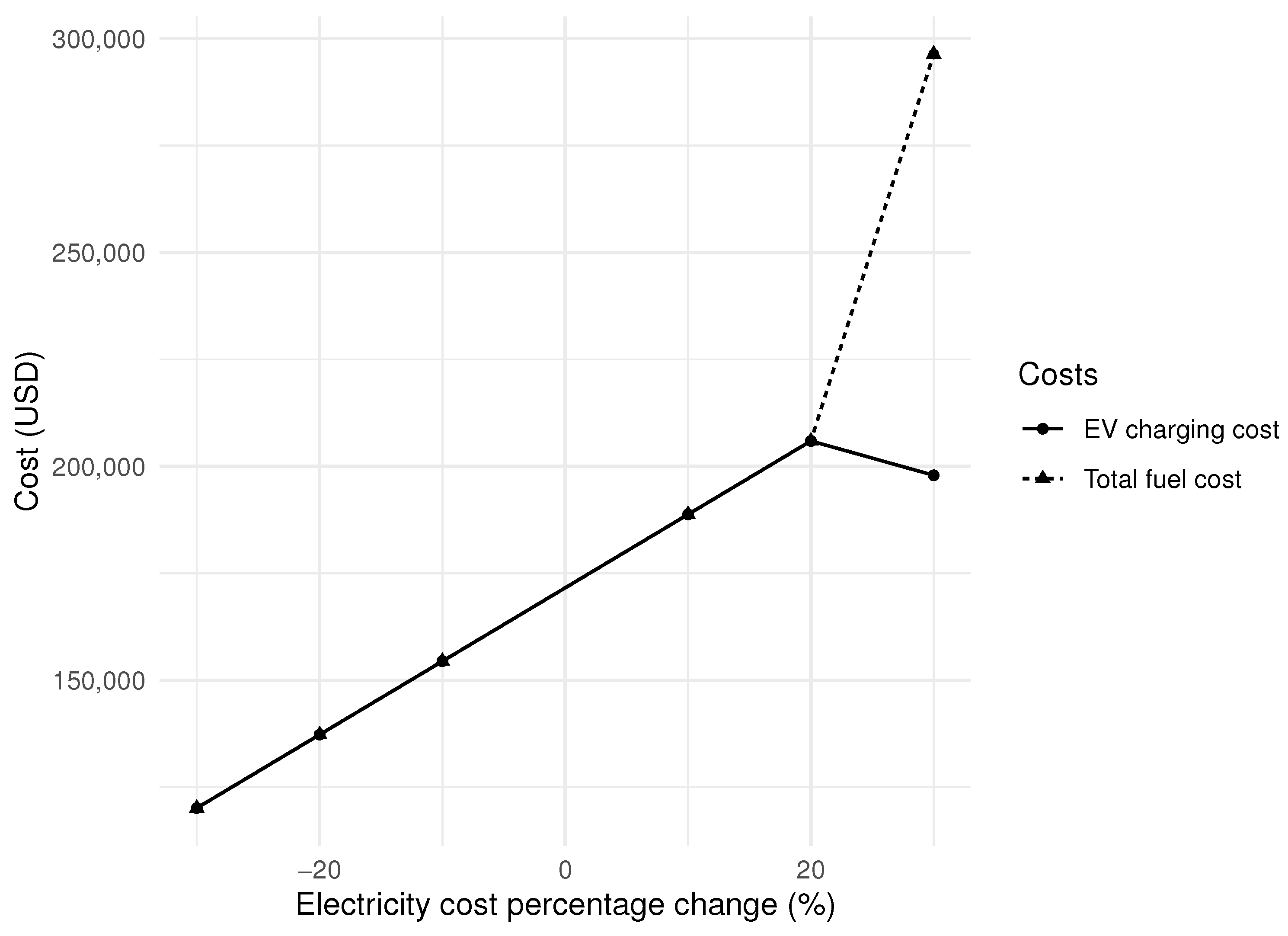
The results of each scenario for the respective cost range are compared to the Baseline scenario costs. In scenario 1 we test the effects of applying a variable electricity cost for EV charging. The change in the electricity cost ranges from to compared to the Baseline electricity cost. Table 3 shows that the model is responsive to the electricity cost change since the total fuel cost changes similarly to the electricity cost change. For example, when the electricity cost is decreased by 30% the total fuel cost is decreased by 30%. As seen in Figure 2 at the 30% increase in the electricity cost the total fuel cost increases by 73%, which is not equivalent to the electricity cost change. That difference occurs because at this cost change the number of ICEVs increases from 0 to 30, which leads to the introduction of the gasoline cost.
In scenario 2, we test the effects of applying a variable gasoline cost for ICEV refueling. The change in the gasoline cost ranges from to compared to the Baseline gasoline cost. Table 4 shows that the model is responsive to the gasoline cost change since the total fuel cost decreases when the gasoline cost decreases. The total fuel cost decreases more than the gasoline cost because the number of ICEVs, that use gasoline, increases compared to the baseline when the gasoline cost decreases. In this scenario, the increase in the gasoline cost stabilizes the total fuel cost and the ICEV refueling cost (Figure 3). Specifically, when the gasoline cost increases the model chooses zero ICEVs and hence the ICEV refueling cost becomes zero. This leads to having a stable total fuel cost that consists only of the EV charging cost, which does not change because in this scenario the electricity cost stays the same. The reason the total fuel cost does not change when the gasoline cost increases is that the model chooses 0 ICEVs because the gasoline cost is too high. This choice leads to the total fuel cost being equal to the electricity cost, which does not change in this scenario.
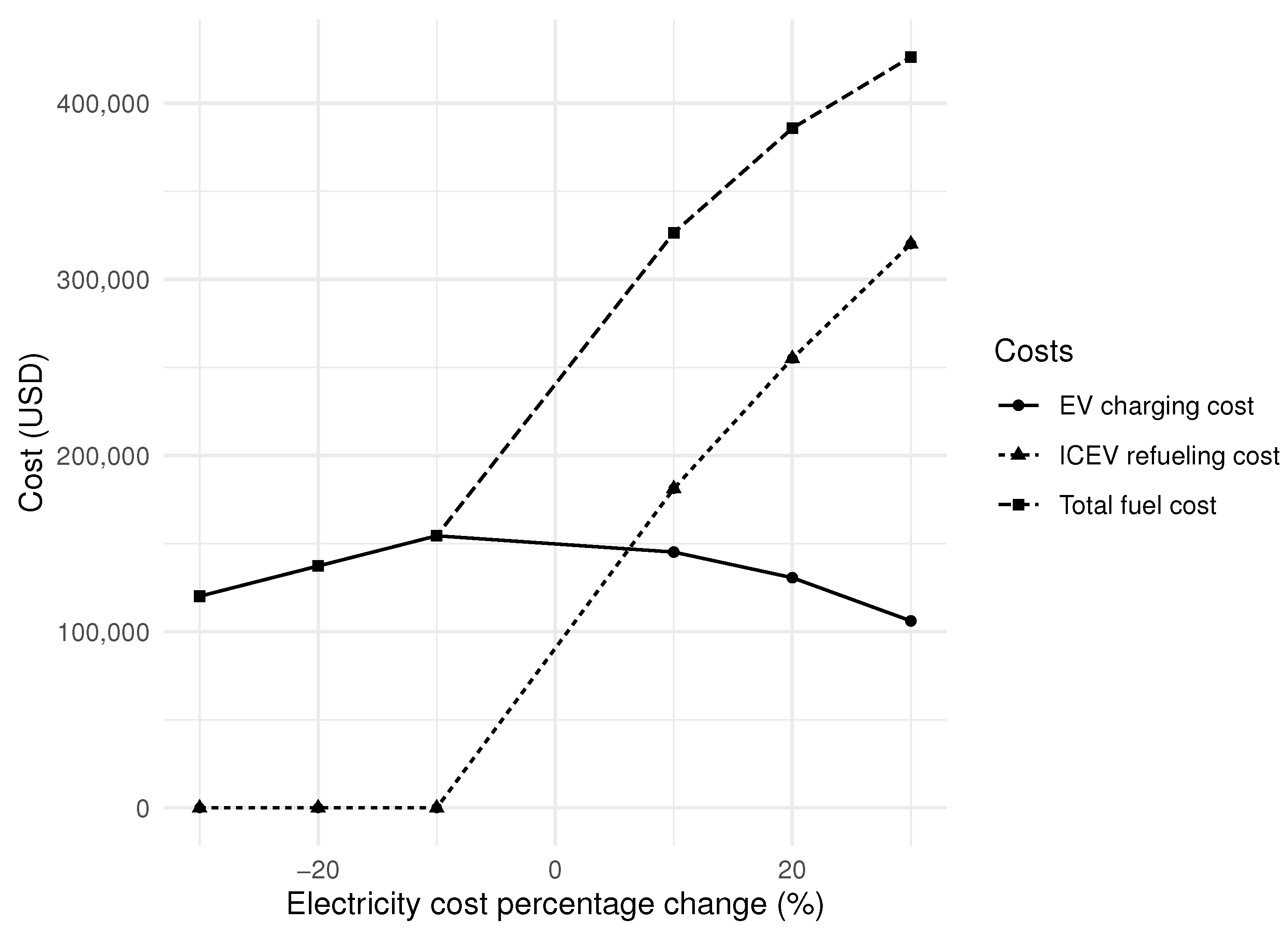
In scenario 3, we test the effects of applying simultaneously variable gasoline and electricity costs for EV recharging and ICEV refueling. The change in the gasoline electricity costs ranges from to compared to the Baseline costs. In this scenario the gasoline cost increases while the electricity cost decreases. Table 5 shows that the model is responsive to the gasoline and electricity cost change since the total fuel cost changes similarly to the gasoline and electricity cost change. When the gasoline cost is increased by 30% and the electricity cost is decreased by 30% the total fuel cost is decreased by 30% because in this case, the model chooses 0 ICEVs. When the electricity cost increases and gasoline cost decreases the total fuel cost increases because the recharging cost increases and the refueling cost is included because ICEVs are introduced in the fleet (Figure 4). Figure 4 shows that the increase in the electricity cost, and simultaneous decrease in gasoline cost, results in an increase in the ICEV refueling and the total fuel costs and a decrease in the EV charging cost. This change happens because the model chooses fewer EVs and more ICEVs.
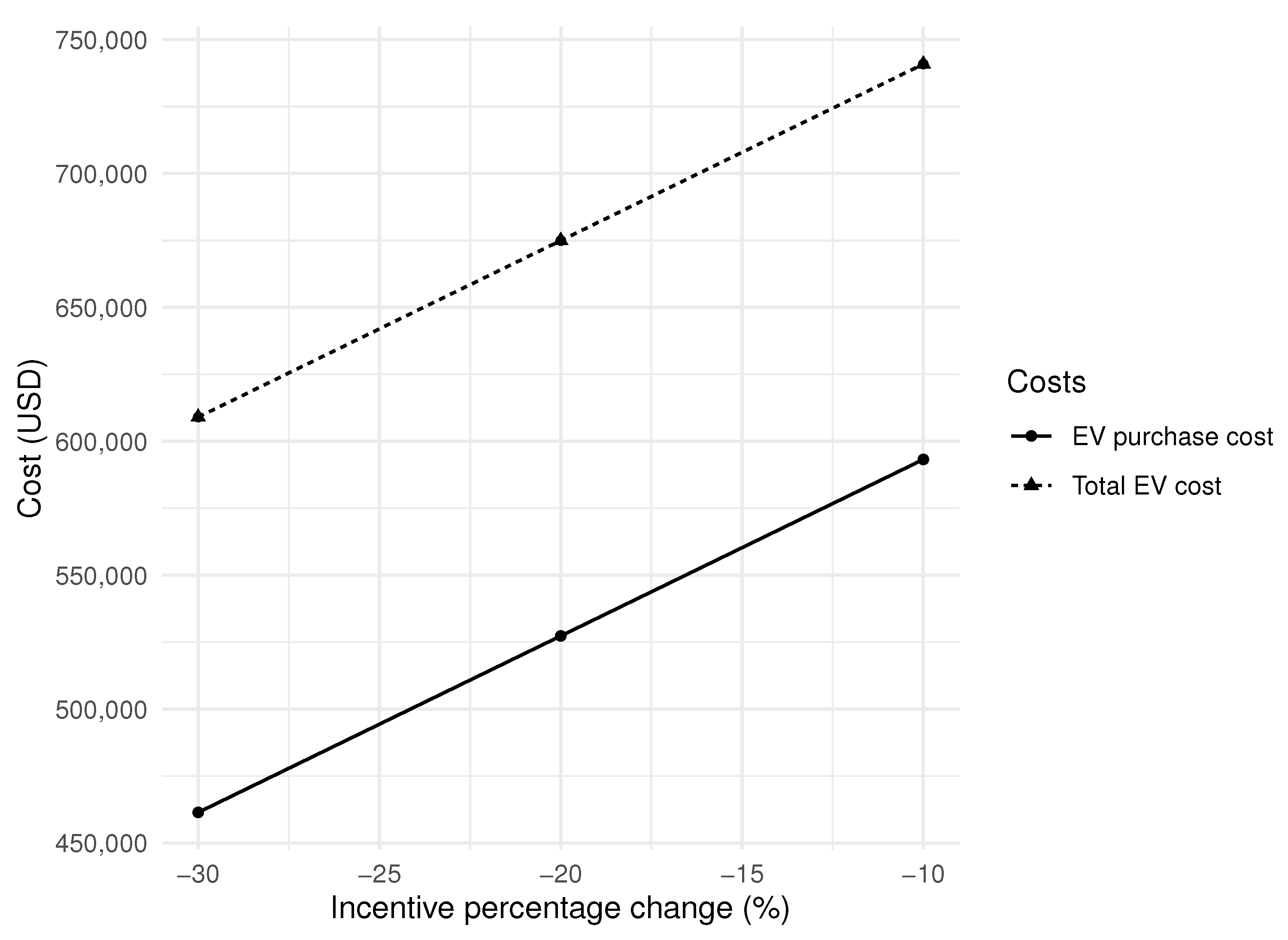
Scenario 4 tests the effects of applying a variable incentive that decreases the EV purchase cost. The change in the EV purchase cost ranges from to compared to the Baseline EV purchase cost. Table 6 shows that the model is responsive to the incentive change since the total EV cost changes similarly to the EV purchase cost change. Specifically, the total EV cost change is decreased by 25% when the EV purchase cost is decreased by 30%. Figure 5 shows that the total EV cost increases accordingly to the EV purchase cost.
5.2. Planning Decisions
The planning decisions shown in this study are the vehicle share and the allocation of the chosen vehicles, as well as the allocation of the charging stations. Table 7 shows that vehicle share changes depending on the scenario and the tested variable external costs (i.e., gasoline, electricity, EV purchase costs). In the Baseline the model optimal EV share is 100% because in Seattle the gasoline cost is high, the electricity cost is low, and the distances are short enough for EVs to complete with a single full charge. In Scenario 1, the EV share decreases to 84.4% only when the electricity cost increases by 30%. In Scenario 2, the EV share decreases as the gasoline cost decreases and it stays the same as the Baseline as the gasoline cost increases. The lower gasoline cost makes ICEVs competitive against the initial investment cost needed for EVs. In Scenario 3, the EV share decreases when the electricity cost increases and the gasoline cost decreases, while it stays the same for the rest of the cost changes.
Furthermore, in both Scenarios 2 and 3, the increase in the gasoline cost does not change the EV share because it is already 100% and cannot increase any further. This shows that the electricity cost in Seattle is low enough to be competitive against the high price of gasoline for ICEVs. This is an expected result because although the cost of purchasing EVs and EV chargers is high compared to the purchase cost of ICEVs, the large difference between the electricity and gasoline costs (Table 1) does not favor ICEVs for the annual mileage of vans that operate in last mile. In Scenario 4, the EV share remains 100% because the incentive would only reinforce the adoption of EVs.
The vehicle share change for the different electricity and gasoline prices shows that the model decisions for the optimal number of EVs and ICEVs will vary according to the fuel prices in different states. Table 8 shows the example of the states with the lowest and highest gasoline prices in the U.S. The gasoline price difference from Mississippi to Washington is . Table 9 shows the example of the states with the lowest and highest electricity prices in the U.S. The electricity price difference from Hawaii to Washington is .
5.3. Model Application across the US
In this section, we test the model in 4 additional US cities to understand how city-specific conditions affect the optimal number of EVs. The goal of the model application across the US is not to compare the results for each city but to understand the changes in EV share. The selected cities represent a selection of different ranges of fuel costs and hub-to-demand node distances. We chose four cities in the US that have different combinations of high miles vs. low miles (i.e., hub-to-demand node distances) and high price spread vs. low price spread. Price spread is the difference between the gasoline price and electricity price in a city. The cities we chose to test and represent these categories are Dallas, New York City, Portland, and San Diego (Table 10). Table 11 shows the gasoline price per gallon, the electricity price per kWh, and the price spread for each city. The gasoline price ranges from $3.42/gallon in Dallas to $5.79/gallon in Portland, while the electricity price ranges from $0.0194/kWh in Dallas to $0.1965 in Portland. The cities with a higher price spread are San Diego (4.6005) and Portland (5.5935)., and the cities with the lower price spread are Dallas (3.3286) and New York City (3.7689) Table 12 shows the average hub-to-demand node distance for each city. The cities with longer distances are San Diego (19 miles) and Dallas (18.5 miles) while the cities with shorter distances are New York City (9.1 miles) and Portland (9.4 miles).
Table 13, Table 14, Table 15 and Table 16 show the optimal number of EVs and ICEVs chosen by the model and the EV share in all the scenarios for each of the cities tested.
In the case of Dallas, which is a city with high miles and low price spread, the baseline EV share is 2.1%. The EV share for Dallas is low because the low gasoline price favors ICEVs and EVs cannot cover the whole network. The reason EVs cannot cover the whole network is that the hub-to-demand node distances are long and the range of the EVs with one full charge is not enough to travel to all the demand nodes. In scenario 1, we see that the EV share for Dallas increases compared to the baseline when the electricity cost decreases, and decreases when the electricity cost increases. In scenario 2, we see that the EV share decreases compared to the baseline when the gasoline cost decreases, and increases when the gasoline cost increases. The increase of the EV share is bigger in scenario 2 compared to scenario 1, when the gasoline and electricity costs change respectively. The reason for the difference in the EV share change is that the gasoline cost is significantly higher than the electricity cost and therefore has a higher effect on the results. In scenario 3, the increase of the EV share is bigger compared to scenarios 1 and 2, when the gasoline cost increases and the electricity cost decreases. The reason for this change is that both the gasoline and electricity costs change at the same time, leading to even smaller charging costs compared to refueling costs. In scenario 4, the EV share increases compared to the baseline as the incentive increases (i.e., EV purchasing cost decreases), because the lower EV purchasing cost along with the low electricity price makes EVs more competitive.
In the case of New York City, which is a city with low miles and a low price spread, the baseline EV share is 0%. The EV share for New York City is 0 because it has a combination of low gasoline prices and relatively high electricity prices. Although, EVs can cover the shorter hub-to-demand node distances the high price spread does not favor EVs. In scenario 1, we see that the EV share increases compared to the baseline when the electricity cost decreases, and stays the same when the electricity cost increases. In scenario 2, we see that the EV share increases when the gasoline cost increases. Again, the increase of the EV share is bigger in scenario 2 compared to scenario 1, when the gasoline and electricity costs change respectively. In scenario 3, the increase of the EV share is bigger compared to scenarios 1 and 2, when the gasoline cost increases and the electricity cost decreases. The EV share stays the same with the baseline when the electricity cost increases and gasoline cost decreases because it is already 0 and cannot decrease any further. In scenario 4, the EV share increases compared to the baseline as the incentive increases (i.e., EV purchasing cost decreases). Specifically, the decrease of the EV purchasing cost by 30% produces one of the highest EV shares for New York City.
In the case of Portland, which is a city with low miles and a high price spread, the baseline EV share is 4.3%. The EV share for Portland is higher compared to the rest of the cities tested because it has the highest gasoline prices and shorter hub-to-demand node distances. The EVs can cover the shorter hub-to-demand node distances with low charging prices. Although the EV share in Portland is higher it is still low because the initial investment cost (EV purchasing and EV charger purchasing costs) for EVs is high. In scenario 1, we see that the EV share increases compared to the baseline when the electricity cost decreases, and stays the same when the electricity cost increases. In scenario 2, we see that the EV share increases when the gasoline cost increases and decreases when the gasoline cost decreases. In scenario 3, the EV share increases when the gasoline cost increases and the electricity cost decreases. For Portland, the change in the electricity and gasoline costs leads to 100% EV share for low electricity and high gasoline costs and 0% for high electricity and low gasoline costs. The reason is that Portland has a low price spread and low miles, which means that a change in fuel prices can have a greater effect on the results. Specifically, the total fuel cost has a lower spread for moving ICEVs and EVs in a network with shorter distances. In scenario 4, the model chooses only EVs when an incentive is introduced (i.e., EV purchasing cost decreases). When the EV purchase cost decreases EVs become competitive against ICEVs, because the cost to refuel EVs is the highest in the cities examined.
In the case of San Diego, which is a city with high miles and a high price spread, the baseline EV share is 0.8%. The EV share for San Diego is low because it has a high gasoline price and longer hub-to-demand node distances. In scenario 1, we see that the EV share increases compared to the baseline when the electricity cost decreases, and decreases when the electricity cost increases. In scenario 2, we see that the EV share increases when the gasoline cost increases and decreases when the gasoline cost decreases. In scenario 3, the EV share increases when the gasoline cost increases and the electricity cost decreases. For San Diego, the change in the electricity and gasoline costs leads to 100% EV share for any increase in the gasoline cost and 0% for any decrease in the gasoline costs. In scenario 4, the model chooses only EVs when an incentive is introduced (i.e., EV purchasing cost decreases). Similarly to Portland, when the EV purchase cost decreases EVs become competitive against ICEVs, because the cost to refuel EVs is the second highest in the cities examined.
6. Discussion
In the discussion section, we aim to show how the changes in external costs affect the optimal EV share, present the factors that can affect EV share but are not included in this study, and mention the public implications of the application of the proposed model by delivery companies.
The results of this study show that changes in electricity and gasoline costs can change the optimal EV share. This is apparent in Table 7 and Table 13, Table 14, Table 15 and Table 16, where we see that the EV share increases when the gasoline cost increases and the electricity cost decreases. While this is true for all cities, the EV share changes vary for different cost changes in each city. For example, in Seattle, the EV share decreases only when the electricity cost increases by 30%, while in Portland the EV share decreases at a 10% electricity cost increase. Although the EV share changes when the fuel cost changes, it is not only based on external costs but also on the distances traveled by vehicles. The effect of the traveled distances can be seen in the testing of Dallas, New York City, Portland, and San Diego, which represent different networks with long and short distances. In these results, we see that in the context of our study, where EVs charge only once overnight, longer distances (e.g., Dallas, San Diego) favor ICEVs, since they have enough fuel capacity (traveling range) to travel in the network. This is seen both in the Baseline and the scenarios because the changes in the EV share are not the same as the changes in the gasoline and electricity costs. The vehicle share decisions made by the proposed model, in both the Seattle case study and the 4 US cities, show that transitioning to EVs is beneficial in terms of cost for freight companies that operate in the last mile when the gasoline cost is high, the electricity cost is low, or there are EV purchasing incentives. Depending on the network the effect of these costs can have a different magnitude on the EV share. Specifically, for cities with shorter hub-to-demand node distances (e.g., New York City, Portland) the gasoline and electricity costs have a smaller effect on the EV share (Table 14 and Table 15).
It is important to note that there are factors, other than EV and EV charging station costs, that hinder EV adoption and are not captured in this model. These factors are the low EV freight supply compared to the demand [9,44], the reliability of EVs in terms of vehicle range for companies that have hubs located further away from the demand compared to the tested case study [8], the uncertainty on which sustainable transportation solutions will be supported in the future by regulations and local conditions [45], and making new operational decisions such as routing and vehicle allocation to support EVs [45].
Understanding how EV-related policies can affect EV adoption by last-mile delivery companies can help federal and local entities (i.e., DOTs, utility companies, etc.) make informed decisions about the initiatives they want to provide. The cases of Dallas, New York City, Portland, and San Diego (Table 13, Table 14, Table 15 and Table 16) show that the EV share is increased when vehicle purchasing incentives are applied. This result means that EV adoption can be increased when EV incentives are introduced. An example of EV-related planning decisions by local entities is that utility companies will need to identify their freight vehicle electrification support goals. They can achieve that by deciding if they plan to support further freight fleet electrification and the purchasing of more EVs. This decision is essential because it can determine the pricing schemes and incentives set by utilities for commercial EVs.
7. Conclusions
More and more commercial fleets have started purchasing EVs or are interested in using EVs for their transportation operations. Most of the companies that use or plan to use EVs will have a mixed fleet with a combination of EVs and ICEVs. Many reasons contribute to the introduction of mixed freight fleets, such as wanting to test a smaller number of vehicles before changing the whole fleet, the high cost of EVs, and EV availability in the market. Operating a mixed freight fleet with EVs and ICEVs will require freight companies to make planning decisions based on their operations. One of the main decisions the companies have to make is how to plan for the long-term effects of mixed fleets, which in this study is the infrastructure changes needed to accommodate the new vehicles.
This study proposes an optimization model that answers the questions (Table 17): What is the best fleet composition?; At which hubs should we assign the new EVs and charging stations? Additionally, we explore the effects of changes in external factors on the long-term planning decisions for mixed fleets. The inputs for the case study network (distribution hubs and demand nodes) are derived from a dataset from an online retail and distribution company operating in Seattle, the King County neighborhood centers dataset. To explore the effects of external factors on the model choices on the fleet composition and EV charger assignment we tested four scenarios. In each scenario, we tested either a change in one of the cost inputs or a change in the charging strategies. Furthermore, we applied the model in 4 cities across the US to understand the effects of the network and fuel costs on the EV share. The model is simple enough to be adopted by most freight companies, regardless of their size, because it is easy to solve and requires the use of easily accessible data.
The results of the study show that EVs are beneficial for last-mile freight companies when gasoline costs are high, electricity costs are low, or there are EV purchasing incentives but there are still barriers that hinder EV adoption. Additionally, the results show that the EV share is affected by both the fuel and purchasing costs and the network distances. The insights from the results of this study can help freight companies identify what are the best long-term planning decisions for a mixed fleet when considering the changes in strategies and costs. Furthermore, the results can be useful for utilities to understand how incentives and gasoline/charging costs can affect EV fleet share and EV charger spatial distribution. This could help utilities prepare for surges in electricity demand in certain locations or estimate how their strategies will affect commercial EV purchases.
Future work on this topic can explore more scenarios, such as changes in customer demand and grid capacity based on location. Testing these additional scenarios could help explore the effects of external factors in combination with spatial changes. Another suggestion for future studies is to explore more solution approaches for the optimization model, other than a commercial solver. A heuristic can be applied to decrease the time the model needs to find the optimal solution.
Author Contributions
Conceptualization, P.G., A.R. and A.G.; methodology, P.G., A.R. and A.G.; analysis, P.G.; data curation, P.G.; writing—original draft preparation, P.G.; writing—review and editing, P.G., A.R. and A.G. All authors have read and agreed to the published version of the manuscript.
Funding
This research received no external funding.
Institutional Review Board Statement
Not applicable.
Informed Consent Statement
Not applicable.
Data Availability Statement
3rd Party Data Restrictions apply to the availability of these data. Data was obtained from a third party and there is no permission to make them available to the public.
Conflicts of Interest
The authors declare no conflict of interest.
References
- Amazon’s 2021 Sustainability Report. 2021. Available online: https://sustainability.aboutamazon.com/2021-sustainability-report.pdf (accessed on 5 April 2024).
- FedEx, Charged up about Our Future. 2022. Available online: https://www.fedex.com/en-us/sustainability/electric-vehicles.html (accessed on 7 May 2023).
- UPS, Sustainable Services, Electrifying Our Future. 2022. Available online: https://about.ups.com/us/en/social-impact/environment/sustainable-services/electric-vehicles—about-ups.html (accessed on 7 May 2023).
- USPS Intends to Deploy over 66,000 Electric Vehicles by 2028, Making One of the Largest Electric Vehicle Fleets in the Nation. 2022. Available online: https://about.usps.com/newsroom/national-releases/2022/1220-usps-intends-to-deploy-over-66000-electric-vehicles-by-2028.htm (accessed on 7 May 2023).
- Gonzalez, J.N.; Gomez, J.; Vassallo, J.M. Do urban parking restrictions and Low Emission Zones encourage a greener mobility? Transp. Res. Part D Transp. Environ. 2022, 107, 103319. [Google Scholar] [CrossRef]
- Figliozzi, M.A.; Boudart, J.A.; Feng, W. Economic and Environmental Optimization of Vehicle Fleets: Impact of Policy, Market, Utilization, and Technological Factors. Transp. Res. Rec. 2011, 2252, 1–6. [Google Scholar] [CrossRef]
- Chen, Z.; Carrel, A.L.; Gore, C.; Shi, W. Environmental and economic impact of electric vehicle adoption in the U.S. Environ. Res. Lett. 2021, 16, 045011. [Google Scholar] [CrossRef]
- İmre, Ş.; Çelebi, D.; Koca, F. Understanding barriers and enablers of electric vehicles in urban freight transport: Addressing stakeholder needs in Turkey. Sustain. Cities Soc. 2021, 68, 102794. [Google Scholar] [CrossRef]
- Tarei, P.K.; Chand, P.; Gupta, H. Barriers to the adoption of electric vehicles: Evidence from India. J. Clean. Prod. 2021, 291, 125847. [Google Scholar] [CrossRef]
- Mehar, S.; Zeadally, S.; Rémy, G.; Senouci, S.M. Sustainable Transportation Management System for a Fleet of Electric Vehicles. IEEE Trans. Intell. Transp. Syst. 2015, 16, 1401–1414. [Google Scholar] [CrossRef]
- Feng, W.; Figliozzi, M.A. Conventional vs. Electric Commercial Vehicle Fleets: A Case Study of Economic and Technological Factors Affecting the Competitiveness of Electric Commercial Vehicles in the USA. Procedia-Soc. Behav. Sci. 2012, 39, 702–711. [Google Scholar] [CrossRef]
- Laporte, G.; Nobert, Y. An exact algorithm for minimizing routing and operating costs in depot location. Eur. J. Oper. Res. 1981, 6, 224–226. [Google Scholar] [CrossRef]
- Murtagh, B.A.; Niwattisyawong, S.R. An Efficient Method for the Multi-Depot Location-Allocation Problem. J. Oper. Res. Soc. 1982, 33, 629–634. [Google Scholar]
- Gendron, B.; Crainic, T.G. A branch-and-bound algorithm for depot location and container fleet management. Locat. Sci. 1995, 3, 39–53. [Google Scholar] [CrossRef]
- Campbell, J.F. Hub Location and the p-Hub Median Problem. Oper. Res. 1996, 44, 923–935. [Google Scholar] [CrossRef]
- Bourbeau, B.; Gabriel Crainic, T.; Gendron, B. Branch-and-bound parallelization strategies applied to a depot location and container fleet management problem. Parallel Comput. 2000, 26, 27–46. [Google Scholar] [CrossRef]
- Taherkhani, G.; Alumur, S.A. Profit maximizing hub location problems. Omega 2019, 86, 1–15. [Google Scholar] [CrossRef]
- Çağrı, K.; Bektaş, T.; Jabali, O.; Laporte, G. The impact of depot location, fleet composition and routing on emissions in city logistics. Transp. Res. Part B Methodol. 2016, 84, 81–102. [Google Scholar] [CrossRef]
- Mohammadi, M.; Torabi, S.; Tavakkoli-Moghaddam, R. Sustainable hub location under mixed uncertainty. Transp. Res. Part E Logist. Transp. Rev. 2014, 62, 89–115. [Google Scholar] [CrossRef]
- Anderluh, A.; Hemmelmayr, V.C.; Rüdiger, D. Analytic hierarchy process for city hub location selection—The Viennese case. Transp. Res. Procedia 2020, 46, 77–84. [Google Scholar] [CrossRef]
- Charting the Course for Early Truck Electrification. 2022. Available online: https://rmi.org/insight/electrify-trucking (accessed on 6 April 2024).
- Ahani, P.; Arantes, A.; Melo, S. A portfolio approach for optimal fleet replacement toward sustainable urban freight transportation. Transp. Res. Part D Transp. Environ. 2016, 48, 357–368. [Google Scholar] [CrossRef]
- Sayarshad, H.R.; Mahmoodian, V.; Bojović, N. Dynamic Inventory Routing and Pricing Problem with a Mixed Fleet of Electric and Conventional Urban Freight Vehicles. Sustainability 2021, 13, 6703. [Google Scholar] [CrossRef]
- Hiermann, G.; Hartl, R.F.; Puchinger, J.; Vidal, T. Routing a Mix of Conventional, Plug-in Hybrid, and Electric Vehicles. HAL 2019, 272, 235–248. [Google Scholar] [CrossRef]
- Goeke, D.; Schneider, M. Routing a mixed fleet of electric and conventional vehicles. Eur. J. Oper. Res. 2015, 245, 81–99. [Google Scholar] [CrossRef]
- All-New, All-Electric E-Transit Custom from Ford Pro Is Set to Spark the EV Revolution for Small Businesses. 2022. Available online: https://media.ford.com/content/fordmedia/feu/en/news/2022/09/08/all-new–all-electric-e-transit-custom-from-ford-pro-is-set-to-s. (accessed on 16 December 2022).
- Metro Neighborhoods in King County. 2012. Available online: https://www5.kingcounty.gov/sdc/Metadata.aspx?Layer=neighborhood (accessed on 6 March 2023).
- Koordinates US Cities GIS Data. 2023. Available online: https://koordinates.com/data/ (accessed on 28 October 2023).
- Distance on a Sphere: The Haversine Formula. 2017. Available online: https://community.esri.com/t5/coordinate-reference-systems-blog/distance-on-a-sphere-the-haversine-formula (accessed on 6 March 2023).
- Washington State Profiles and Energy Estimates. 2023. Available online: https://www.eia.gov/state/?sid=WA#tabs-4 (accessed on 1 May 2023).
- Nicholas, M. Estimating Electric Vehicle Charging Infrastructure Costs Across Major U.S. Metropolitan Areas; ICCT: Washington, DC, USA, 2019. [Google Scholar]
- Electric Vehicle Charging Speeds—U.S. Department of Transportation. 2023. Available online: https://www.transportation.gov/rural/ev/toolkit/ev-basics/charging-speeds (accessed on 1 May 2023).
- Business Rates—City of Seattle. 2023. Available online: https://www.seattle.gov/city-light/business-solutions/business-billing-and-account-information/business-rates#burienseatacshorelineandunincorporatedkingcountybusinesses (accessed on 1 May 2023).
- Petroleum and Other Liquids—U.S. Energy Information Administration. 2023. Available online: https://www.eia.gov/dnav/pet/hist/LeafHandler.ashx?n=pet&s=emm_epmru_pte_y48se_dpg&f=m (accessed on 1 May 2023).
- Fuel Economy—U.S. Department of Energy. 2022. Available online: https://www.fueleconomy.gov/feg/noframes/44952.shtml (accessed on 1 May 2023).
- How Many Miles & Years Do Ford Transits Last? (8 Important Facts). 2020. Available online: https://motorandwheels.com/do-ford-transits-last-long/ (accessed on 7 June 2023).
- Electric Vehicle Charger Maintenance Basics. 2022. Available online: https://www.365pronto.com/blog/electric-vehicle-charger-maintenance (accessed on 7 June 2023).
- How Many Miles Will A Mercedes Metris Last? 2023. Available online: https://vehq.com/how-many-miles-will-a-mercedes-metris-last/ (accessed on 7 June 2023).
- US Electricity Profile 2021. 2022. Available online: https://www.eia.gov/electricity/state/ (accessed on 1 August 2023).
- State Gas Price Averages. 2023. Available online: https://gasprices.aaa.com/state-gas-price-averages/ (accessed on 1 August 2023).
- 2017 Mercedes-Benz Metris Passenger Van Review. 2017. Available online: https://www.automoblog.net/2017-mercedes-benz-metris-passenger-van-review/ (accessed on 7 July 2023).
- Amazon.com Announces Fourth Quarter Results. 2023. Available online: https://ir.aboutamazon.com/news-release/news-release-details/2023/Amazon.com-Announces-Fourth-Quarter-Results/default.aspx (accessed on 25 July 2023).
- Bestuzheva, K.; Besançon, M.; Chen, W.K.; Chmiela, A.; Donkiewicz, T.; van Doornmalen, J.; Eifler, L.; Gaul, O.; Gamrath, G.; Gleixner, A.; et al. The SCIP Optimization Suite 8.0. arXiv 2021, arXiv:2112.08872. [Google Scholar]
- Alp, O.; Tan, T.; Udenio, M. Transitioning to sustainable freight transportation by integrating fleet replacement and charging infrastructure decisions. Omega 2022, 109, 102595. [Google Scholar] [CrossRef]
- Melander, L.; Nyquist-Magnusson, C.; Wallström, H. Drivers for and barriers to electric freight vehicle adoption in Stockholm. Transp. Res. Part D Transp. Environ. 2022, 108, 103317. [Google Scholar] [CrossRef]
Figure 1.
Visual outline for the long-term planning network.

Figure 2.
Sensitivity analysis for Scenario 1—EV charging and total fuel costs change over the electricity cost change.
Figure 2.
Sensitivity analysis for Scenario 1—EV charging and total fuel costs change over the electricity cost change.

Figure 3.
Sensitivity analysis for Scenario 2—ICEV refueling and total fuel costs change over the gasoline cost change.
Figure 3.
Sensitivity analysis for Scenario 2—ICEV refueling and total fuel costs change over the gasoline cost change.
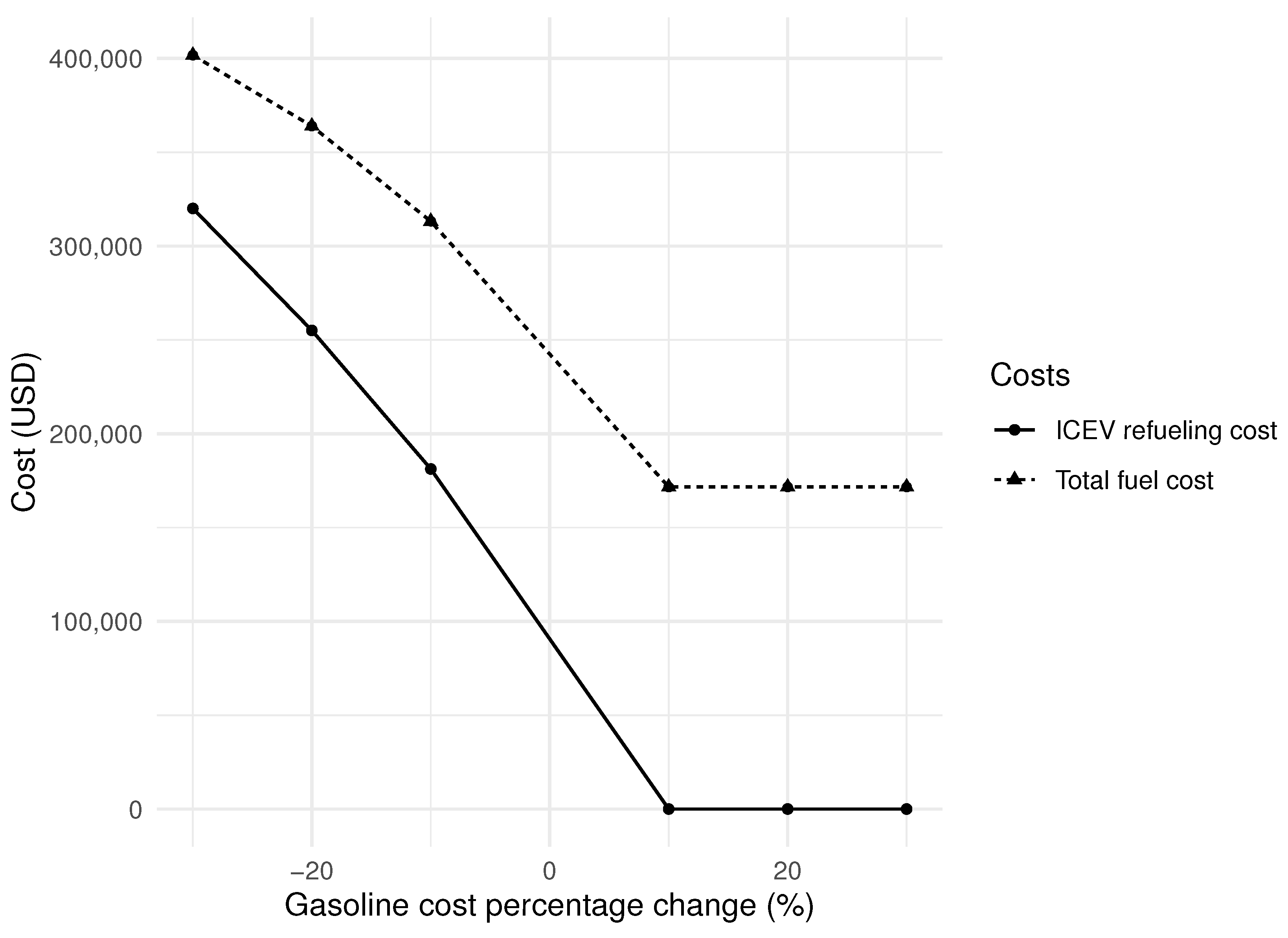
Figure 4.
Sensitivity analysis for Scenario 3—EV charging, ICEV refueling, and total fuel costs change over the electricity cost change.
Figure 4.
Sensitivity analysis for Scenario 3—EV charging, ICEV refueling, and total fuel costs change over the electricity cost change.

Figure 5.
Sensitivity analysis for Scenario 4—EV purchase and total EV costs change over the incentive change.
Figure 5.
Sensitivity analysis for Scenario 4—EV purchase and total EV costs change over the incentive change.


Table 1.
Data inputs.
| Parameters | Values | Units | Source |
|---|---|---|---|
| 15 | years | [36] | |
| 14 | years | [38] | |
| 10 | years | [37] | |
| 7,548,000,000 × 12 | kWh/year | [30] | |
| 5432 | USD | [31] | |
| 49,575 | USD/vehicle | [26] | |
| 37,960 | kWh/one full charge per day for a year | [26] | |
| USD/mile | [33] | ||
| USD/mile | [34] | ||
| 14,205 | USD/vehicle | [36] | |
| 25,200 | USD/vehicle | [38] | |
| 33,000 | USD/vehicle | [41] | |
| 4000 | USD/charger | [37] | |
| 5500 | USD | [42] |
Table 2.
Long-term planning model testing scenarios.
| Scenario | Description | |
|---|---|---|
| Baseline | All inputs are used as presented in the Section 2.2 | |
| External cost | Scenario 1 | Electricity cost is variable |
| External cost | Scenario 2 | Gasoline cost is variable |
| External cost | Scenario 3 | Electricity and gasoline costs are variable |
| Incentive | Scenario 4 | EV purchase cost incentive is variable |
Table 3.
Long-term planning model sensitivity analysis—Scenario 1.
| Scenario | EV Charging Cost (USD) | ICEV Refueling Cost (USD) | Total Fuel Cost (USD) | Total Fuel Cost Change (%) |
|---|---|---|---|---|
| Baseline | 171,622.9 | 0 | 171,622.9 | 0 |
| Scenario 1 | ||||
| Electricity cost change (%) | ||||
| −30 | 120,136.0 | 0 | 120,136.0 | −30 |
| −20 | 137,298.3 | 0 | 137,298.3 | −20 |
| −10 | 154,460.6 | 0 | 154,460.6 | −10 |
| +10 | 188,785.2 | 0 | 188,785.2 | +10 |
| +20 | 205,947.4 | 0 | 205,947.4 | +20 |
| +30 | 197,929.0 | 98,444.3 | 296,373.2 | +73 |
Table 4.
Long-term planning model sensitivity analysis—Scenario 2.
| Scenario | EV Charging Cost (USD) | ICEV Refueling Cost (USD) | Total Fuel Cost (USD) | Total Fuel Cost Change (%) |
|---|---|---|---|---|
| Baseline | 171,622.9 | 0 | 171,622.9 | 0% |
| Scenario 2 | ||||
| Gasoline cost change (%) | ||||
| −30 | 81,651.0 | 320,088.2 | 401,739.2 | −134 |
| −20 | 108,884.0 | 255,088.7 | 363,972.8 | −112 |
| −10 | 132,003.9 | 181,222.0 | 313,225.8 | −83 |
| +10 | 171,622.9 | 0 | 171,622.9 | 0 |
| +20 | 171,622.9 | 0 | 171,622.9 | 0 |
| +30 | 171,622.9 | 0 | 171,622.9 | 0 |
Table 5.
Long-term planning model sensitivity analysis—Scenario 3.
| Scenario | EV Charging Cost (USD) | ICEV Refueling Cost (USD) | Total Fuel Cost (USD) | Total Fuel Cost Change (%) | |
|---|---|---|---|---|---|
| Baseline | 171,622.9 | 0 | 171,622.9 | 0% | |
| Scenario 3 | |||||
| Electricity cost change (%) | Gasoline cost change (%) | ||||
| −30 | +30 | 120,136.0 | 0 | 120,136.0 | −30 |
| −20 | +20 | 137,298.3 | 0 | 137,298.3 | −20 |
| −10 | +10 | 154,460.6 | 0 | 154,460.6 | −10 |
| +10 | −10 | 145,204.3 | 181,222.0 | 326,426.2 | +90 |
| +20 | −20 | 130,660.8 | 255,088.7 | 385,749.6 | +125 |
| +30 | −30 | 106,146.3 | 320,088.2 | 426,234.5 | +148 |
Table 6.
Long-term planning model sensitivity analysis—Scenario 4.
| Scenario | EV Maintenance Cost (USD) | EV Purchase Cost (USD) | Total EV Cost (USD) | Total EV Cost Change (%) |
|---|---|---|---|---|
| Baseline | 147,648 | 659,136 | 806,784 | 0 |
| Scenario 4 | ||||
| Incentive—EV cost change (%) | ||||
| −30 | 147,648.0 | 461,395.2 | 609,043.2 | −25 |
| −20 | 147,648.0 | 527,308.8 | 674,956.8 | −16 |
| −10 | 147,648.0 | 593,222.4 | 740,870.4 | −8 |
Table 7.
Vehicle share for all scenarios—Seattle.
| Scenario | Number of EVs | Number of ICEVs | EV Share (%) | |
|---|---|---|---|---|
| Baseline | 192 | 0 | 100 | |
| Scenario 1 | ||||
| Electricity cost change (%) | ||||
| −30 | 192 | 0 | 100 | |
| −20 | 192 | 0 | 100 | |
| −10 | 192 | 0 | 100 | |
| +10 | 192 | 0 | 100 | |
| +20 | 192 | 0 | 100 | |
| +30 | 162 | 30 | 84.4 | |
| Scenario 2 | ||||
| Gasoline cost change (%) | ||||
| −30 | 72 | 120 | 37.5 | |
| −20 | 102 | 90 | 53.1 | |
| −10 | 132 | 60 | 68.8 | |
| +10 | 192 | 0 | 100 | |
| +20 | 192 | 0 | 100 | |
| +30 | 192 | 0 | 100 | |
| Scenario 3 | ||||
| Electricity cost change (%) | Gasoline cost change (%) | |||
| −30 | +30 | 192 | 0 | 100 |
| −20 | +20 | 192 | 0 | 100 |
| −10 | +10 | 192 | 0 | 100 |
| +10 | −10 | 132 | 60 | 68.8 |
| +20 | −20 | 102 | 90 | 53.1 |
| +30 | −30 | 72 | 120 | 37.5 |
| Scenario 4 | ||||
| Incentive—EV cost change (%) | ||||
| −30 | 192 | 0 | 100 | |
| −20 | 192 | 0 | 100 | |
| −10 | 192 | 0 | 100 | |
Table 8.
Highest and lowest gasoline prices in the U.S. compared to WA [40].
Table 8.
Highest and lowest gasoline prices in the U.S. compared to WA [40].
| State | Gasoline Prices per Gallon | Difference to WA (%) |
|---|---|---|
| Washington | $4.950 | 0 |
| Mississippi | $3.253 | −41.38 |
| California | $4.998 | +0.97 |
Table 9.
Highest and lowest electricity prices in the U.S. compared to WA [39].
Table 9.
Highest and lowest electricity prices in the U.S. compared to WA [39].
| State | Electricity Prices per kWh | Difference to WA (%) |
|---|---|---|
| Washington | $0.0875 | 0 |
| Idaho | $0.0817 | −6.86 |
| Hawaii | $0.3031 | +110.39 |
Table 10.
US cities examined.
| High Miles | Low Miles | |
|---|---|---|
| High price spread | San Diego | Portland |
| Low price spread | Dallas | New York City |
Table 11.
Price spread for each city.
| City | Gasoline Price ($/gallon) | Electricity Price ($/kWh) | Price Spread |
|---|---|---|---|
| Dallas | 3.42 | 0.0914 | 3.3286 |
| New York City | 3.93 | 0.1611 | 3.7689 |
| Portland | 5.79 | 0.1965 | 5.5935 |
| San Diego | 4.69 | 0.0895 | 4.6005 |
Table 12.
Average hub-to-demand node distances for each city.
| City | Average Distance (Miles) |
|---|---|
| Dallas | 18.5 |
| New York City | 9.1 |
| Portland | 9.4 |
| San Diego | 19.0 |
Table 13.
Vehicle share for all scenarios—Dallas.
| Scenario | Number of EVs | Number of ICEVs | EV Share (%) | |
|---|---|---|---|---|
| Baseline | 3 | 137 | 2.1 | |
| Scenario 1 | ||||
| Electricity cost change (%) | ||||
| −30 | 20 | 120 | 14.3 | |
| −20 | 20 | 120 | 14.3 | |
| −10 | 3 | 137 | 2.1 | |
| +10 | 3 | 137 | 2.1 | |
| +20 | 2 | 138 | 1.4 | |
| +30 | 1 | 139 | 0.7 | |
| Scenario 2 | ||||
| Gasoline cost change (%) | ||||
| −30 | 0 | 140 | 0 | |
| −20 | 0 | 140 | 0 | |
| −10 | 1 | 139 | 0.7 | |
| +10 | 20 | 120 | 14.3 | |
| +20 | 50 | 90 | 35.7 | |
| +30 | 110 | 30 | 78.6 | |
| Scenario 3 | ||||
| Electricity cost change (%) | Gasoline cost change (%) | |||
| −30 | +30 | 140 | 0 | 100 |
| −20 | +20 | 80 | 60 | 57.1 |
| −10 | +10 | 20 | 120 | 14.3 |
| +10 | −10 | 0 | 140 | 0 |
| +20 | −20 | 0 | 140 | 0 |
| +30 | −30 | 0 | 140 | 0 |
| Scenario 4 | ||||
| Incentive—EV cost change (%) | ||||
| −30 | 140 | 0 | 100 | |
| −20 | 80 | 60 | 57.1 | |
| −10 | 20 | 120 | 14.3 | |
Table 14.
Vehicle share for all scenarios—New York City.
| Scenario | Number of EVs | Number of ICEVs | EV Share (%) | |
|---|---|---|---|---|
| Baseline | 0 | 116 | 0 | |
| Scenario 1 | ||||
| Electricity cost change (%) | ||||
| −30 | 2 | 114 | 1.7 | |
| −20 | 2 | 114 | 1.7 | |
| −10 | 0 | 116 | 0 | |
| +10 | 0 | 116 | 0 | |
| +20 | 0 | 116 | 0 | |
| +30 | 0 | 116 | 0 | |
| Scenario 2 | ||||
| Gasoline cost change (%) | ||||
| −30 | 0 | 116 | 0 | |
| −20 | 0 | 116 | 0 | |
| −10 | 0 | 116 | 0 | |
| +10 | 2 | 114 | 1.7 | |
| +20 | 2 | 114 | 1.7 | |
| +30 | 26 | 90 | 22.4 | |
| Scenario 3 | ||||
| Electricity cost change (%) | Gasoline cost change (%) | |||
| −30 | +30 | 86 | 30 | 74.1 |
| −20 | +20 | 26 | 90 | 22.4 |
| −10 | +10 | 2 | 114 | 1.7 |
| +10 | −10 | 0 | 116 | 0 |
| +20 | −20 | 0 | 116 | 0 |
| +30 | −30 | 0 | 116 | 0 |
| Scenario 4 | ||||
| Incentive—EV cost change (%) | ||||
| −30 | 86 | 30 | 74.1 | |
| −20 | 2 | 114 | 1.7 | |
| −10 | 1 | 115 | 0.9 | |
Table 15.
Vehicle share for all scenarios—Portland.
| Scenario | Number of EVs | Number of ICEVs | EV Share (%) | |
|---|---|---|---|---|
| Baseline | 4 | 90 | 4.3 | |
| Scenario 1 | ||||
| Electricity cost change (%) | ||||
| −30 | 94 | 0 | 100 | |
| −20 | 94 | 0 | 100 | |
| −10 | 34 | 60 | 36.2 | |
| +10 | 4 | 90 | 4.3 | |
| +20 | 4 | 90 | 4.3 | |
| +30 | 4 | 90 | 4.3 | |
| Scenario 2 | ||||
| Gasoline cost change (%) | ||||
| −30 | 0 | 94 | 0 | |
| −20 | 0 | 94 | 0 | |
| −10 | 1 | 93 | 1.1 | |
| +10 | 94 | 0 | 100 | |
| +20 | 94 | 0 | 100 | |
| +30 | 94 | 0 | 100 | |
| Scenario 3 | ||||
| Electricity cost change (%) | Gasoline cost change (%) | |||
| −30 | +30 | 94 | 0 | 100 |
| −20 | +20 | 94 | 0 | 100 |
| −10 | +10 | 94 | 0 | 100 |
| +10 | −10 | 1 | 93 | 1.1 |
| +20 | −20 | 0 | 94 | 0 |
| +30 | −30 | 0 | 94 | 0 |
| Scenario 4 | ||||
| Incentive—EV cost change (%) | ||||
| −30 | 94 | 0 | 100 | |
| −20 | 94 | 0 | 100 | |
| −10 | 94 | 0 | 100 | |
Table 16.
Vehicle share for all scenarios—San Diego.
| Scenario | Number of EVs | Number of ICEVs | EV Share (%) | |
|---|---|---|---|---|
| Baseline | 1 | 123 | 0.8 | |
| Scenario 1 | ||||
| Electricity cost change (%) | ||||
| −30 | 124 | 0 | 100 | |
| −20 | 124 | 0 | 100 | |
| −10 | 34 | 90 | 27.4 | |
| +10 | 1 | 123 | 0.8 | |
| +20 | 0 | 124 | 0 | |
| +30 | 0 | 124 | 0 | |
| Scenario 2 | ||||
| Gasoline cost change (%) | ||||
| −30 | 0 | 124 | 0 | |
| −20 | 0 | 124 | 0 | |
| −10 | 0 | 124 | 0 | |
| +10 | 124 | 0 | 100 | |
| +20 | 124 | 0 | 100 | |
| +30 | 124 | 0 | 100 | |
| Scenario 3 | ||||
| Electricity cost change (%) | Gasoline cost change (%) | |||
| −30 | +30 | 124 | 0 | 100 |
| −20 | +20 | 124 | 0 | 100 |
| −10 | +10 | 124 | 0 | 100 |
| +10 | −10 | 0 | 124 | 0 |
| +20 | −20 | 0 | 124 | 0 |
| +30 | −30 | 0 | 124 | 0 |
| Scenario 4 | ||||
| Incentive—EV cost change (%) | ||||
| −30 | 124 | 0 | 100 | |
| −20 | 124 | 0 | 100 | |
| −10 | 124 | 0 | 100 | |
Table 17.
Summary of study results.
| Research Question | Study Conclusions/Results |
|---|---|
| What is the best fleet composition? | The fleet composition is affected by the gasoline and electricity costs, and the distances traveled by vehicles. |
| At which hubs should we assign the new EVs and charging stations? | The hubs selected for the placement of EV chargers and EVs are the ones closest to demand nodes. |
Disclaimer/Publisher’s Note: The statements, opinions and data contained in all publications are solely those of the individual author(s) and contributor(s) and not of MDPI and/or the editor(s). MDPI and/or the editor(s) disclaim responsibility for any injury to people or property resulting from any ideas, methods, instructions or products referred to in the content. |
© 2024 by the authors. Licensee MDPI, Basel, Switzerland. This article is an open access article distributed under the terms and conditions of the Creative Commons Attribution (CC BY) license (https://creativecommons.org/licenses/by/4.0/).
Share and Cite
MDPI and ACS Style
Goulianou, P.; Regan, A.; Goodchild, A. Long-Term Planning for a Mixed Urban Freight Fleet with EVs and ICEVs in the USA. Sustainability 2024, 16, 3144. https://doi.org/10.3390/su16083144
AMA Style
Goulianou P, Regan A, Goodchild A. Long-Term Planning for a Mixed Urban Freight Fleet with EVs and ICEVs in the USA. Sustainability. 2024; 16(8):3144. https://doi.org/10.3390/su16083144
Chicago/Turabian StyleGoulianou, Panagiota, Amelia Regan, and Anne Goodchild. 2024. "Long-Term Planning for a Mixed Urban Freight Fleet with EVs and ICEVs in the USA" Sustainability 16, no. 8: 3144. https://doi.org/10.3390/su16083144
Note that from the first issue of 2016, this journal uses article numbers instead of page numbers. See further details here.