Soft Actor-Critic and Risk Assessment-Based Reinforcement Learning Method for Ship Path Planning

Abstract

Ship path planning is one of the most important themes in waterway transportation, which is deemed as the cleanest mode of transportation due to its environmentally friendly and energy-efficient nature. A path-planning method that combines the soft actor-critic (SAC) and navigation risk assessment is proposed to address ship path planning in complex water environments. Specifically, a continuous environment model is established based on the Markov decision process (MDP), which considers the characteristics of the ship path-planning problem. To enhance the algorithm’s performance, an information detection strategy for restricted navigation areas is employed to improve state space, converting absolute bearing into relative bearing. Additionally, a risk penalty based on the navigation risk assessment model is introduced to ensure path safety while imposing potential energy rewards regarding navigation distance and turning angle. Finally, experimental results obtained from a navigation simulation environment verify the robustness of the proposed method. The results also demonstrate that the proposed algorithm achieves a smaller path length and sum of turning angles with safety and fuel economy improvement compared with traditional methods such as RRT (rapidly exploring random tree) and DQN (deep Q-network).

1. Introduction

Waterway transportation is an important mode of transportation with the advantages of low costs and strong capacity, which is different from road and railway transportation. With the trend of globalization, maritime containerized trade has been rapidly increasing over the past two decades [1]. Concurrently, inland waterway transportation has also developed rapidly, becoming a competitive alternative to and complement of road and rail transport [2]. However, there are frequent safety accidents in water transportation [3]. According to statistics, the Suez Canal carries 30% of the world’s container traffic, and about 12% of the world’s trade passes through this waterway. In January 2023, the cargo ship “MV GLORY” ran aground on the canal due to errors in route planning and improper operation by the operator. The heavy cargo ship “Ever Given” also ran aground in the canal in March 2021, causing a major blockage that affected about USD 60 billion in trade. Path-planning failures can cause significant damage, not only leading to ship’s hull damage and obstructing or even blocking waterways, but also resulting in oil spills and environmental pollution [4], and may even lead to casualties. These failures result in major safety and economic losses.

Ship path planning must ensure the safety of waterway transportation while taking into account the factors of efficiency, economy, etc. As the logistics industry accelerates its transformation and upgrading to digitalization and intelligence, waterway transportation is also gradually moving toward modernization and intelligence, and intelligent navigation of ships is one of the important issues. The intelligent navigation system of a ship consists of several modules, such as a perception and situation understanding module, a decision and planning module, a motion control and execution module, and a communication module [5]. Path planning is the key sub-module of the decision and planning module. Reasonable ship path planning considering navigation safety and economy can reduce costs and improve transportation efficiency at the same time.

The ship path-planning problem aims at finding the optimal path from a start point to a target point in each navigational environment under various constraints and environmental limitations. Current research on path planning mainly uses traditional methods, which make it difficult to learn a generalized planning strategy, and the deep reinforcement learning methods which are popular in the robotics field are rarely applied to the ship path-planning problem. Therefore, the research in this paper has practical value and theoretical reference significance for improving the ship’s path-planning ability. The contributions of this study can be specified as follows.

(1) Aiming at the ship path-planning problem under a continuous environment, this study constructs a state-continuous environment model based on the Markov decision process to avoid errors caused by the discrete processing of maps.

(2) The risk assessment model is applied to improve the state space and convert the absolute bearing information into relative information. And the action space considers the limitations of the ship course, which guides the path-planning strategy to optimize towards high smoothness.

(3) The SAC algorithm framework based on maximum entropy reinforcement learning is used to design the path-planning algorithm, balancing exploration and utilization in a continuous environment, designing distance and angle potential rewards based on sparse rewards, and introducing a risk penalty term to ensure path safety.

2. Related Works

According to the principle of the method, path-planning methods can be divided into search mechanism-based, bionic evolution-based, sampling mechanism-based, and reinforcement learning methods. As one of the classical heuristic search algorithms, the A-star algorithm is widely used in path planning. However, the traditional A* algorithm has shortcomings, including a long search time and too many redundant nodes [6]. Therefore, He et al. [7] improved the A-star algorithm by considering the dynamic search mechanism of the time factor so that the ship can generate a more reasonable dynamic obstacle avoidance path. Zhen et al. [8] analyzed the factors that affect ship navigation safety and designed the turning model and smoothing method to improve the A-star algorithm so that the path could effectively avoid the shallow water area. Liang et al. [9] improved the A-star algorithm by setting a safe distance from obstacles and removing unnecessary waypoints. Song et al. [10] introduced the weights of distance, energy, and time to generate paths with different costs, using attraction and repulsion fields to improve the cost estimation function of the A* algorithm. The evolutionary algorithm is a global path-planning method with high adaptability and robustness. Huang et al. [11] established a mathematical model for ship route planning with the target point of the shortest ship sailing time and used the ant colony algorithm to optimize the initial ship path. Zhao et al. [12] proposed a hybrid ship path-planning method based on an improved particle swarm optimization–genetic algorithm, which not only has fast convergence, but also improves the diversity of solutions. Tsou et al. [13] and Dong et al. [14] utilized ant algorithms to develop ship path-planning techniques with the aim of achieving optimal energy consumption. Search-based methods can only optimize paths in a finite search space, and evolutionary algorithms need to encode the space. Thus, these two types of methods both have limitations and are only applicable to discretized environments.

The sampling-based method is suitable for solving path-planning problems in continuous environments as it avoids the need for environment discretization processing. Cao et al. [15] proposed an improved RRT algorithm including path shearing and smoothing modules which considered the safe distance between a moving ship and an obstacle. The algorithm’s feasibility was verified through experiments in two kinds of inland river scenarios. However, the research did not address the limitation of turning angles during ship navigation, which resulted in poor path smoothing. Liu et al. [16] presented a hybrid probabilistic roadmap (HPRM) algorithm for ship route planning, which improves the utilization of sampling points via the sampling point reset (SPR) function and reduces the number of ship turns via the Douglas–Peucker (D-P) algorithm.

The above traditional path-planning methods are unable to fully utilize the historical experience and have difficulty learning a generalized strategy due to the lack of autonomous learning capability without a data replay mechanism. In recent years, with the development and application of artificial intelligence technology, reinforcement learning has provided a new method for path planning that confronts the unsatisfactory results of traditional methods, does not rely on accurate environment models, and has a significant advantage in solving efficiency. Zhao et al. [17] proposed a Q-learning path-planning algorithm for autonomous underwater vehicles (AUVs) using a potential-game-based optimal rigid graph method to balance the trade-off between energy consumption and network robustness. Chen et al. [18] regularized distances, obstacles, and prohibited areas as rewards or penalties, and used Q-learning to learn an action-reward model that allows ships to find navigation strategies.

Deep reinforcement learning is suitable for path-planning problems through function approximation and representation learning of path-planning strategies using deep neural networks [19]. Guo et al. [20] modeled the environment using the grid method and optimized the reward function of DQN by setting the potential energy reward of the target to the ship, adding a reward region near the target and a danger region near the obstacles, which allowed the ship to avoid obstacles and reach the target point faster. Luo et al. [21] proposed a reinforcement learning algorithm for single AGV path planning. The algorithm uses the A* algorithm to guide the DQN algorithm, leading to a faster training process and less time needed for decision making compared with using only the A* algorithm. However, this method requires pre-gridding of the environment and the state space is discrete, which makes it simple to implement but will cause some loss of accuracy compared with continuous environments. Li et al. [22] improved the action space and reward function of the DQN algorithm by using the artificial potential field method based on the continuous state space, which learns an effective strategy. Zheng et al. [23] proposed an improved dense reward of the PPO method for ship route guidance. The method has high training efficiency and decision accuracy, enabling safe and efficient path decisions in complex and uncertain environments. The disadvantage of the above methods is that they only consider the minimization of distance in the evaluation index, without fully investigating the generalization of the model. Dong et al. [24] addressed the robot path-planning problem using the DDPG algorithmic framework and an adaptive exploration method based on the ε-greedy algorithm to improve exploration efficiency. Zhao et al. [25] improved the stability of the robot’s path-planning algorithm by normalizing the state and adding a Batch Norm layer to the strategy network, but the study only addressed the robot’s path-planning problem.

3. Problem Description and Environmental Modeling

3.1. Ship Path-Planning Problem Description

The ship path-planning problem contains two elements, the map and the ship. The map consists of water boundaries, obstacles, a start point, and a target point. The ship has elements such as the domain of the ship, the safety distance, etc. The water area is represented by rectangular areas of length $L$ and width $W$. A right-angle coordinate system is established with the left boundary of the water area as the $y$-axis and the lower boundary of the water area as the $x$-axis. The water area is represented as $S_{map}=\left\{\left(x,y\right)\right|0<x<L,0<y<W\}$. And the area outside the water area is represented as $S_{out}=\left\{\left(x,y\right)\right|x\le 0 \mathrm{o}\mathrm{r} x\ge L,y\le 0 \mathrm{o}\mathrm{r} y\ge W\}$, which is defined as a restricted navigation area. Obstacles are simplified as circles, and each irregular obstacle expands into a circle of radius $r_i$ whose position in waters is ${(x}_{ri},y_{ri}\left)\right(i\in B=\{\mathrm{0,1},2,\dots ,n\})$, where $B$ is the set of obstacles in the map. The space occupied by the obstacle is also a restricted navigation area for ships, and a path is invalid if it crosses this area.

The ship is the subject of the path-planning problem. The ship domain is simplified as a circle with radius of the safe distance $d$ during ship navigation. Considering that the actual ship is not a particle and will be affected by uncertain environmental factors such as weather, weaves, etc. during navigation, the ship may deviate from the planned trajectory, setting a safe distance to avoid accidents is necessary. Therefore, the solution for ship path planning is a safe path zone rather than a separate path. The center trajectory of the ship’s path at time $t$ is $P=\left\{\left(p_{xt},p_{yt}\right)|t\in \left\{\mathrm{0,1},2,\dots ,T_{end}\right\}\right\}$.

3.2. Markov Decision Processes for the Ship Path-Planning Problem

Reinforcement learning consists of two parts, the agent and the environment. The agent learns the optimal strategy in constant interaction with the environment. The agent is the subject of actions, and various characteristics of the agent in the environment are denoted as state, while the agent can take different actions to obtain a new state after interacting with the environment [26]. The reward mechanism drives the state to make transfers by taking sensible actions so that the agent receives a larger reward value in the environment. The environment in reinforcement learning can generally be described by a Markov decision process (MDP) [27].

The ship path-planning problem can be described as a Markov decision process, represented by $\left(S,A,R,P_{{ss}^{\prime }}^a,\gamma ,\pi \left(a_t|s_t\right),v_{\pi }\left(s\right)\right),$ where $S$ is the set of states and $A$ is the set of actions. After taking the action $a$, the state transitions to $s$, and an instant reward $R\left(s,a\right)$ is obtained. $P_{{ss}^{\prime }}^a$ represents the probability that the state is transferred from $S$ to $S^{\prime }$ when action $a$ is chosen. The cumulative reward of state $S_t$ at moment $t$ is called the return $G_t$. The calculation function is shown as follows, including the instant reward $R_t$ of $S_t$ and the rewards of the subsequent k steps, where $\gamma$ is a discount factor characterizing the degree of reward decay. Agents explore the environment and learn strategy $\pi \left(a_t|s_t\right)$ by interacting with the environment. The value function $v_{\pi }\left(s\right)$ is used to evaluate the merits of the state.

$$G={\sum }_{k=0}^{\infty }{\gamma }^k{R}_{t+k}$$

(1)

The state of the ship in navigation can be described by position and course. Considering the mission objectives of path planning, information on the target point and obstacles should also be included. When an action is taken, the state of the ship’s position and course is updated; meanwhile, the ship is reasonably rewarded for guiding itself toward the target point. The objective of the ship’s path-planning scenario is to optimize the path-planning scheme, i.e., the policy $\pi \left(a_t|s_t\right)$, specifically to maximize the expectation of cumulative return $J\left(\pi \right)$ of the policy. The objective function is calculated as follows:

$$J\left(\pi \right)={\mathbb{E}}_{\pi }\left[{\sum }_{t}r\left(s_t,a_t\right)\right]$$

(2)

3.3. Risk Assessment Model

To guide the algorithm in finding a safer path more quickly in path-planning scenarios with known or unknown obstacles, the restricted navigation information is fully exploited by evaluating the collision risk of the restricted navigation area. The state space is updated using direction and distance information of the restricted navigation area through the restricted navigation area detection strategy. And the reward function is improved based on a risk assessment model in which the path safety factor is increased by introducing a risk penalty.

3.3.1. Detection of Restricted Navigation Area Information

The restricted navigation area includes the area outside the water boundary and the space occupied by the obstacles. Obtaining the position and bearing of the restricted navigation area facilitates the correct decision making in path planning, enabling the ship to avoid obstacles while avoiding entering the shoal area and running aground.

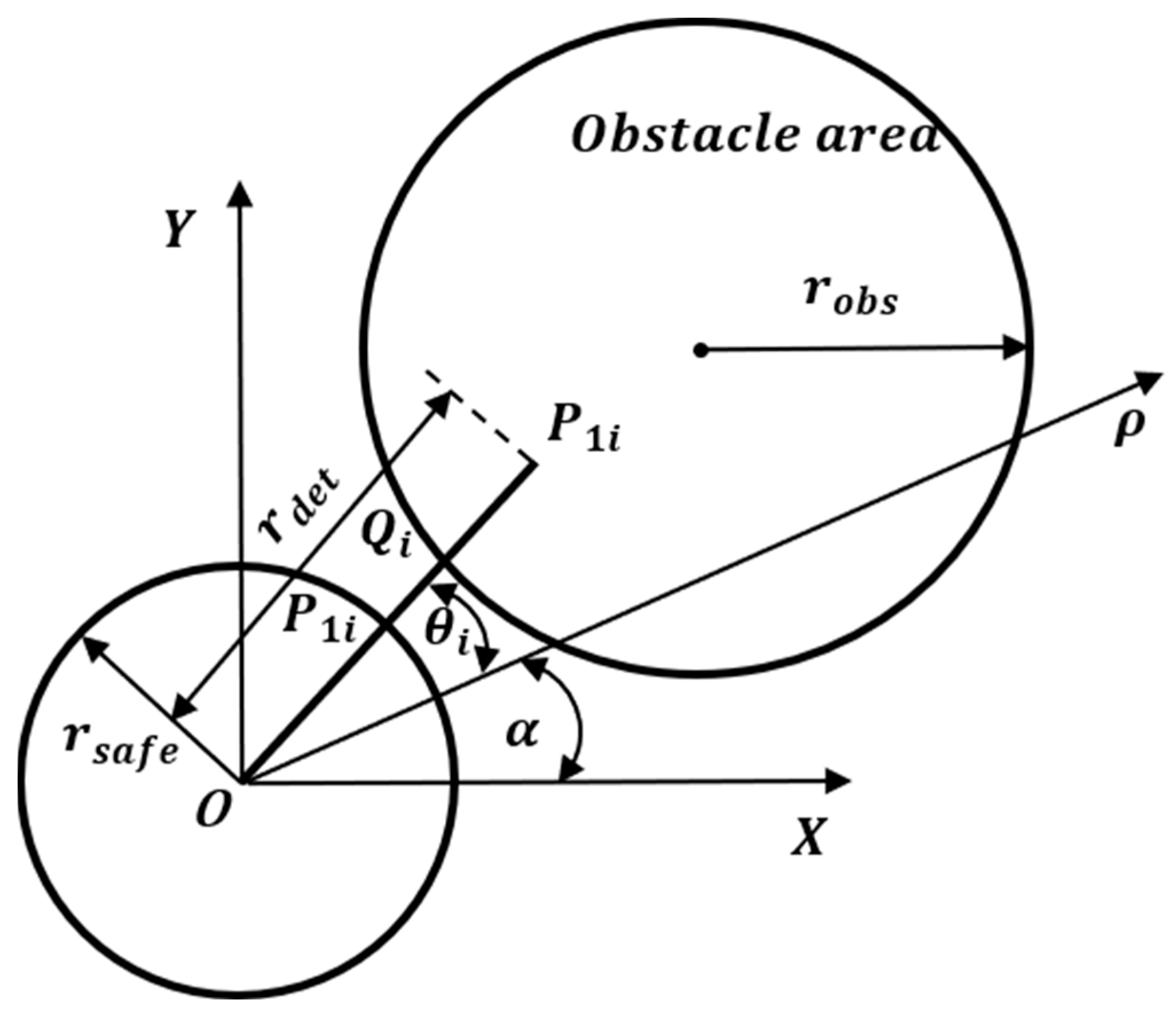
Firstly, the current center position is denoted by $O$, and the current course is denoted by $\mathsf{\alpha }$. A ray $L_o$ is drawn out from the direction of $\mathsf{\alpha }$ with $O$ as the pole and $L_o$ as the polar axis, so that a polar coordinate system $\mathsf{\rho }~\mathsf{\theta }$ is established. Five line segments are utilized to detect the restricted navigation area. The polar equations for the ship safety domain boundary, the detection line segments, and the obstacle boundaries are as follows:

$$\rho =r_{safe}$$

(3)

$$\left\{\begin{array}{c}{r}_{safe}\le \rho \le r_{det}\\ \theta ={\theta }_i,i=\mathrm{1,2},3,\dots ,n\end{array}\right.$$

(4)

$${\rho }^2-2a\cos \theta -2b\sin \theta +a^2+b^2-{r_{obs}}^2=0$$

(5)

In this function, parameter $r_{safe}$ denotes the radius of the ship safety domain; parameter $r_{det}$ denotes the length of the detection line segment; and parameter ${\mathsf{\theta }}_i$ denotes the angle relative to the ship’s course, where $I=\{\mathrm{0,1},2,\dots ,n\}$. Parameter $a$ and parameter $b$ are the location parameters of the center point of the obstacle, and parameter $r_{obs}$ is the radius of the obstacle.

We assume that the two endpoints of the line segment are $P_{1i}$ and $P_{2i}$. If there is an intersection between $L_i$ and the obstacle’s boundary, the intersection point is denoted as $Q_i$, and $l_i$ is returned, which takes the value of the length of the line segment $P_{1i}{Q}_i$. If the line segment $L_i$ does not intersect with the obstacle’s boundary, returning directly to the length $l_i$ of the line segment $L_i$ will result in the same value as the endpoint $P_{2i}$ and intersection point $Q_i$ coincide with each other. This can be easily confused with the case where there is an intersection. As a result, $k_i$ is used as the return value in the end, and it is defined as follows.

$$k_i=\left\{\begin{array}{c}{l}_i,restrictednavigationareadetected\hfill \\ l_i+\epsilon ,norestrictednavigationareadetected\hfill \end{array}\right.$$

(6)

In this formula, parameter $\mathsf{\epsilon }$ is a small positive number relative to $l_i$. The range of values for $\mathsf{\epsilon }$ is $0<\mathsf{\epsilon }\le 0.05l_i$.

The method for detecting information regarding restricted navigation areas outside the boundary is the same as that for obstacle detection. The diagram in Figure 1 shows how to acquire distance information of the restricted navigation area $\left(k_1,k_2,\dots ,k_i,{\dots ,k}_n\right)$ and bearing information $\left({\theta }_1,{\theta }_2,\dots ,{\theta }_i,{\dots ,\theta }_n\right)$.

3.3.2. Navigation Risk Assessment Model

Distance information from different directions can be obtained by detecting restricted navigation areas. To make full use of this information, the data are first normalized. Then, the coefficients of each direction’s information are determined. Finally, a linear summation is performed to obtain a comprehensive risk assessment model. The level of collision risk faced by the ship increases with the assessment value and decreases vice versa. The risk assessment process consists of the following steps:

Step 1: The traversal judgment determines whether there is an intersection between the set of line segments $L_{all}=\left\{{L_1,L_2,\dots ,L}_i,\dots ,L_n\right\}$ and the boundary. If an intersection exists, return $k_i$ and proceed to Step 3. If not, proceed to Step 2.

Step 2: To determine whether the set of detected line segments $L_{all}$ intersects with the obstacle or not, the traversal is performed and $k_i$ is obtained. After this, proceed to Step 3.

Step 3: The risk of collision is calculated using the risk assessment function, which is based on the obtained $K=\left\{{k_{1,}{k}_{2,}\dots ,k}_n\right\}$, with the following formula:

$$A=-{\sum }_{i=1}^n{{\vartheta }_{i}k}_i,$$

(7)

In this formula, the parameter ${\vartheta }_i$ represents the coefficient that corresponds to $k_i$.

It is a great challenge to solve the continuous environment model in reinforcement learning. The ship path-planning model in this study utilizes MDP with continuous state space and considers the safe distance between the ship and obstacles to determine a safe path area. Additionally, a risk assessment model is constructed to evaluate the navigational risk of the ship based on the direction and position of the restricted navigation area obtained from detection. By incorporating the risk assessment model into the path-planning method, the safety of the path can be improved.

4. Path-Planning Algorithm Design

Based on the SAC algorithm framework, a novel path-planning algorithm is proposed, in which this paper specifically considers the limitations of the ship course during navigation when designing the action space so that the safety and smoothness of the path can be increased. To improve the generalization of the model, the ship’s position coordinates relative to the target point, the sine and cosine values of the course angle, and restricted navigation area information are used to construct a continuous state space, which can reduce errors caused by state discretization. Considering the size of the ship domain and the risk assessment model, the reward function is improved by introducing the risk penalty into the sparse reward. Additionally, distance potential energy and angle potential energy rewards are designed to guide path optimization reasonably, which ensures the avoidance of navigation risks and guarantees the quality of the path.

4.1. Action Space Design

A discretization approach is used for the design of the action space in the form of a discrete action space, which is a finite number of actions. To prevent a large turning angle in the path from exceeding the ship’s steering operating range and producing unnecessary fuel consumption, a turning angle limit of ${\theta }_{res}$ is set for each step. The two-dimensional path-planning problem addressed in this paper involves a discrete action space comprising three actions: turning left by ${\theta }_{res}$, maintaining the current state, and turning right by ${\theta }_{res}$. The actions are mutually exclusive, have no temporal correlation, and are limited in number, so the action space can be coded using a three-dimensional one-hot vector, which allows for the conversion of the three categorical variables into numerical vectors. Each action category is represented by a dedicated column or feature in the numerical vector and is converted into a vector consisting of 0 and 1. The encoding positions, respectively, indicate whether the actions have been adopted, where $a_1={\left[\mathrm{1,0,0}\right]}^{\mathrm{T}}$, $a_2={\left[\mathrm{0,1,0}\right]}^{\mathrm{T}}$, and $a_3={\left[\mathrm{0,0,1}\right]}^{\mathrm{T}}$.

4.2. State Space Design

The direct information describing the current position of the ship mainly includes its absolute coordinates, course, the absolute coordinates of the target point, and information on any restricted navigation areas. However, it is difficult to learn the path-planning strategy efficiently if direct information is used as the state. Deep reinforcement learning can fully fit the characteristics of each position and plan paths on a specific map by learning the relationship between absolute location and action selection through a large amount of exploration. But when the target point position changes, the relationship between absolute position and action selection will also change. This leads to the learned strategy becoming invalid and the model losing its generalization ability. To improve the transferability of the state and the generalization of the model, the original state is reprocessed again to create a more concise and efficient representation that still maintains a strong correlation with the reward function. The information processing involves the following three aspects:

• Transform absolute position data into relative target point position data, including relative coordinates, relative distance, and relative direction.
• Set three measuring lines to obtain the information of bearing and distance using the strategy for detecting restricted navigation area information that integrates itself into the state space and combines with the designed action space. The bearing information consists of the directions of the three measuring lines, each corresponding to an angle in the action space. The distance information includes the values obtained by the three measuring lines, representing the restricted navigation area detection information.
• Use the sine and cosine values to represent the course angle data adequately, which are constrained to the range of [−1,1]. The benefits of the above method include not only avoiding standardization processing, but also directly using sine and cosine values to calculate other information, such as the angle between the heading angle and the target guidance line.

4.3. Reward Function Design

In reinforcement learning, the feedback signals received by the agent through interaction with the environment are called rewards, which can be used to improve the strategy through the reward mechanism constantly [28]. In the path-planning task, sparse rewards are designed for the two subtasks, i.e., avoiding restricted navigation areas and reaching the target point from the start point. The reward $R_{goal}$ is obtained when the ship reaches the target point; the penalty $R_{out}$ is obtained when the ship enters the restricted navigation area. And if the ship does not reach the target point and does not enter the restricted navigation area, it continues to navigate and obtains the step penalty $R_{step}$. The ship is encouraged to avoid restricted navigation areas and to reach its target in as few steps as possible.

$$R_s=\left\{\begin{array}{c}{R}_{goal},reachingtarget\hfill \\ R_{out},enteringrestrictednavigationarea\hfill \\ R_{step},keepsailing\hfill \end{array}\right.$$

(8)

This paper designs a potential-guided reward, including a distance potential and an angle potential, to densify the reward. When the ship’s state changes, the reward function can respond quickly to obtain an instant reward so that each state transition of the ship is fully learned, and it helps to avoid excessive exploration. The risk assessment model is also incorporated into the reward function, which imposes penalties on high-risk paths to improve the safety of the algorithm.

1.

Distance Potential Reward

A simpler form of determining the reward is based on the distance of the current position from the target point, but it lacks immediate feedback. The distance potential reward in this paper is defined as a reward if the ship’s current position is closer to the target than its previous position, or a penalty if it is farther away. This form better describes the instant change in distance potential energy and encourages the ship to be more proactive in its approach to the target. The distance potential energy reward expression is shown as follows:

$$R_{dis}={-\omega }_{dis}\left({dis}_{now}-{dis}_{pre}\right)$$

(9)

In this formula, ${dis}_{now}$ and ${dis}_{pre}$ represent the relative distance of the current state and the previous state, respectively. ${\omega }_{dis}$ is the factor of $R_{dis}$.

2.

Angular Potential Reward

The potential energy of the angle is calculated based on the angle $\phi$ between the target guideline and the current course angle, which is in the range of [$0,\pi$], where the target guidance line is the line connecting the ship’s current position and the target, representing the ship’s expected course. The formula for this reward is as follows:

$$R_{angel}={\omega }_{angel}\mathsf{\Delta }\varphi ={\omega }_{angel}\left(\cos {\phi }_{now}-\cos {\phi }_{pre}\right)$$

(10)

In this formula, ${\phi }_{now}$ represents the angle of the current state, while ${\phi }_{pre}$ represents the angle of the previous state. The variable $\mathsf{\Delta }\varphi$ represents the difference in cosine values between the two given angles. ${\omega }_{angel}$ is the factor of $R_{angel}$. If $∆\varphi >0$, it means that the current angular potential energy is greater than the angular potential energy of the previous moment and should be rewarded. And if $∆\varphi <0$, it means that the current angular potential energy is smaller than the angular potential energy of the previous moment and should be punished.

3.

Penalty for risk assessment

Due to the restricted navigation area information introduced to the state space, the corresponding reward function must be added based on the principle of state and reward co-design. According to the risk assessment model, the risk assessment penalty function is designed as follows:

$$R_{ra}=-\sum _{i=1}^3{{\omega }_{i}s}_i$$

(11)

In this formula, $s_i$ corresponds to the distance data of the restricted navigation area. When the distance is larger, the navigation risk is greater and the penalty should be imposed, and in the end, the restricted navigation area penalty is obtained. And ${\omega }_i$ is the factor of $s_i$. Compared with sparse rewards, the risk penalty $R_{ra}$ enables the ship to learn the strategy of staying away from restricted navigation areas in advance, and the resulting path is safer.

4.4. Algorithmic Framework Based on SAC

The concept of entropy is employed to quantify the level of disorder in system variables [29], and the entropy, i.e., $H\left(\pi \left(·|s_t\right)\right),$ characterizes the extent of randomness in the stochastic strategy $\pi$. There are three advantages of SAC introducing entropy into reinforcement learning: it increases the degree of the strategy’s randomness, strengthens the degree of algorithmic exploration, and prevents the algorithm from becoming trapped in a local optimum or even losing the ability to learn. The parameter of the strategy function is denoted as $\theta$. The entropy value is added to the objective function, which is calculated as follows:

$$J\left(\pi \left(\theta \right)\right)={\mathbb{E}}_{\pi }\left[\sum _{t}r\left(s_t,a_t\right)+\alpha H\left(\pi \left(·|s_t\right)\right)\right]$$

(12)

Policy ${\pi }^{\ast }\left(\theta \right)$ can be obtained from $J\left(\pi \left(\theta \right)\right)$. SAC is an off-policy reinforcement learning method. It stores each step’s state, action, and reward in a replay buffer and approximates the value using randomly selected samples. This process is called experience replay [30]. SAC adopts the actor-critic framework. The actor collects data by interacting with the environment [31], while the critic’s value function directs the actor in learning a more efficient strategy by using a policy-based gradient optimizer [32]. The critic learns a value function to measure the quality of state–action pairs from the data collected by the actor, and then helps the actor to update the policy.

To avoid overestimation of value, one actor network (${\pi }_{\theta }$) and two critic networks ($Q_{{\omega }_1}$ and $Q_{{\omega }_2}$) are constructed. The algorithm’s instability, caused by repeated updates of TD error targets, can be avoided by introducing target networks $Q_{{\omega }_1^{-}}$ and $Q_{{\omega }_2^{-}}$, corresponding to $Q_{{\omega }_1}$ and $Q_{{\omega }_2}$. The target networks all utilize the soft update mechanism [33], which gradually brings the parameters of the critic target network closer to the critic network. This ensures a more reliable convergence of the algorithm. The parameters of the target networks are updated as follows:

$${\omega }_{new}^{-}=\tau \omega +\left(1-\tau \right){\omega }_{old}^{-}$$

(13)

In this formula, $\tau$ represents the soft update factor. ${\omega }_{old}^{-}$ and ${\omega }_{new}^{-}$, respectively, represent the parameters of the target network before and after updating. And $\omega$ represents the parameter of the training network. To prevent inefficiency in the algorithm, this paper’s method uses fully connected neural networks instead of overly complex networks. The ship path-planning algorithm that combines SAC with navigational risk assessment is abbreviated as RA-SAC.

5. Simulation Experiment

5.1. Experimental Setup

The simulation experiment’s hardware platform configuration is Intel Core i7-9700K CPU @ 3.60 GHz (8 CPUs) (Intel, Santa Clara, CA, USA). The programming was implemented on the PyCharm 2021.1.2 platform. The simulation experiment’s map size is 50 × 50, and the algorithm’s parameters are determined through repeated testing. The specific parameter values are listed in

Table 1. Parameters for experiments.

Parameter	Meaning	Value
${lr}_{actor}$	Actor network learning rate	10−4
${lr}_{critic}$	Critic network learning rate	10−3
${dim}_h$	Number of neurons in the hidden layer	128
$\gamma$	Discount factor	0.95
$\tau$	Soft update factor	0.005
$N$	Number of samples for batch gradient descent	128
$L$	Length of detection line in restricted navigation area	2.0
$D$	Radius of ship domain	0.5

.

5.2. Algorithm Validation Experiment

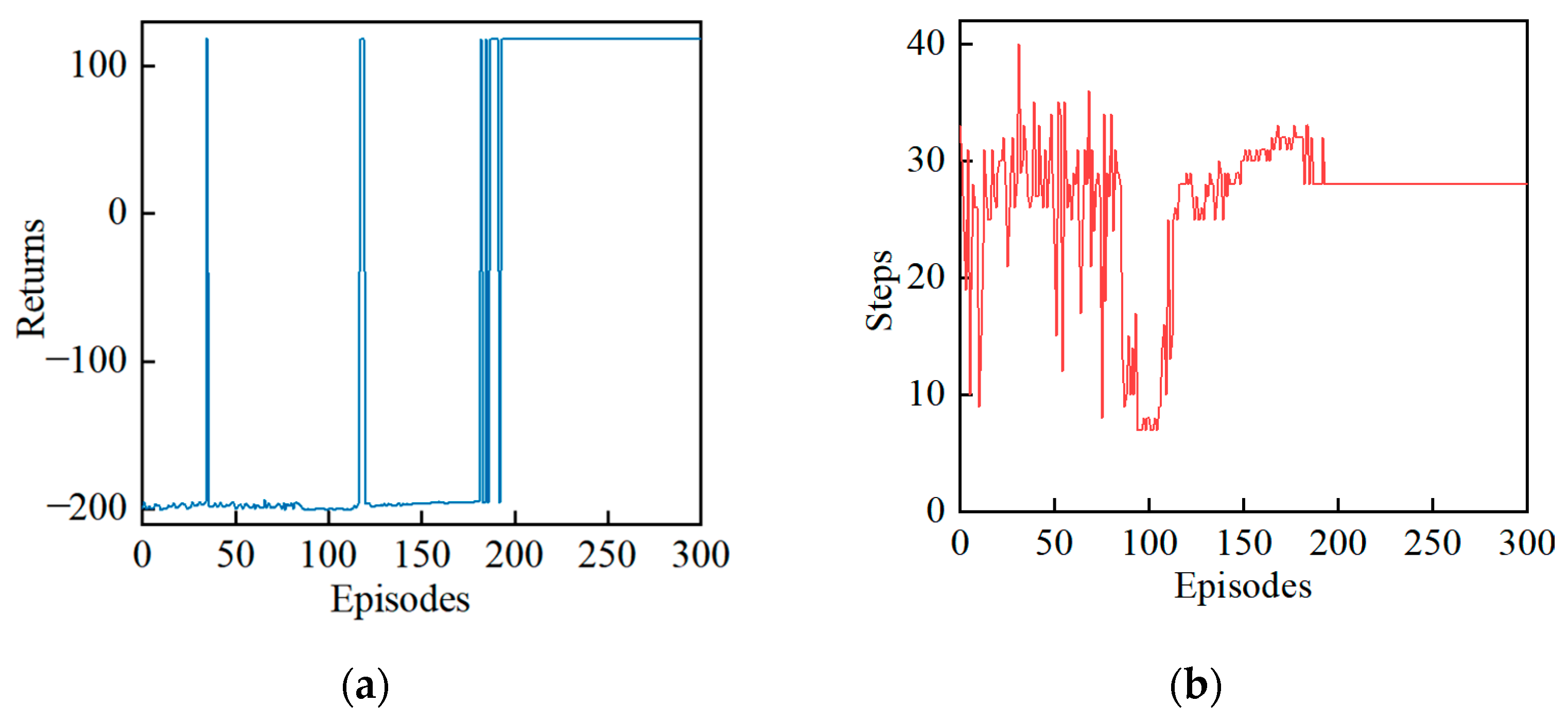
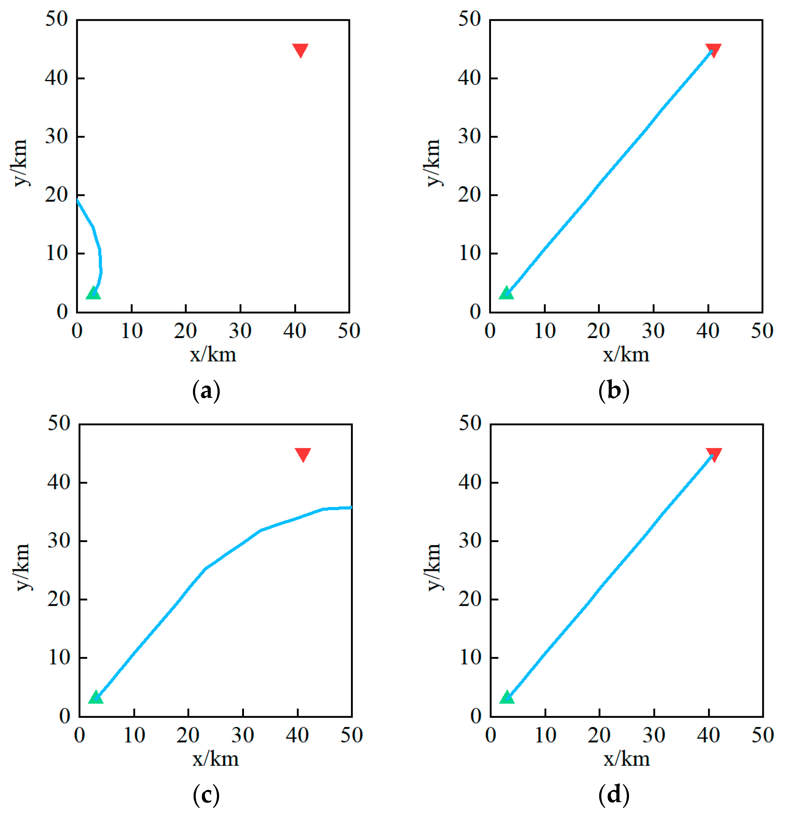
To examine the algorithm’s effectiveness throughout the training process, experiments were conducted in an obstacle-free environment. In Figure 2, the horizontal axis represents the number of training episodes, and the vertical axis represents the return and the number of steps, respectively. Figure 3 shows the trajectory changes after different episodes. The return before training was −200, which means that the ship had not yet learned the path-planning strategy, and at this time, the model used randomly initialized parameters. As the algorithm gradually learned the strategy, the model parameters were continuously optimized, and there was some volatility in the return curve.

After 10 episodes, the ship tried to approach the target point, but it ended up reaching the boundary near the starting point, resulting in a significant penalty and the end of the episode. This shows that the algorithm was still exploring and had not yet explored positive samples. Due to the exploratory mechanism of reinforcement learning, the agent obtains different training samples by continuously interacting with the environment.

After 117 episodes, the ship successfully reached the goal from the starting point and the algorithm collected positive samples that brought a positive return of 118, which helped the agent to learn good strategies. After 150 episodes, the ship reached the boundary near the goal with more steps than in the tenth episode. In this stage, the policy continued to explore based on positive samples, which may have resulted in better or worse samples. These samples were used by the algorithm to learn the path-planning strategy. After 193 episodes, the return curve and step curve converged, and the optimal solution for path planning was obtained. The validation experiments demonstrate the dynamic refinement process of the path-planning policy, which consists of four stages: the exploration stage without positive samples in the early stage, the stage in which positive samples are collected, the exploration stage with positive samples in the later stage, and the stage where the positive samples are utilized with the negative samples to learn the converged strategy.

5.3. Algorithm Performance Comparison Experiments

To verify the effectiveness of RA-SAC in solving the path-planning problem, path-planning comparison experiments with RRT and DQN methods were conducted. The methods can be categorized into deep reinforcement learning-based methods (DQN) and traditional methods (RRT) based on their characteristics. The complexity of the environment could be increased by adding more obstacles while keeping the same map size. Two indicators, path length and turning angle sum, were used to evaluate the path-planning results. Path length characterized the quality of the path-planning result, with shorter paths indicating better economy. Turning angle sum, on the other hand, characterized the safety and economy of the path.

5.3.1. Scenario 1

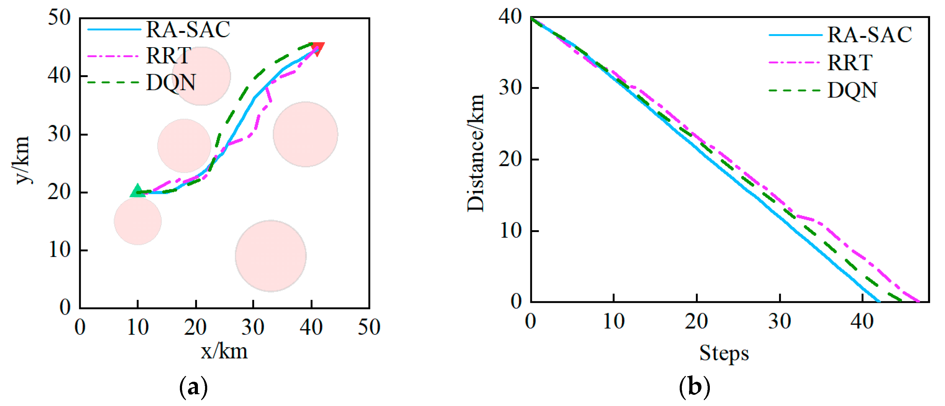
In Scenario 1, five obstacles are randomly generated, with start and target points located at coordinates (10, 20) and (41, 45), respectively. Figure 4 displays the experimental results, which include the trajectory change and the distance curve between the ship and the target. The experimental results indicate that the paths obtained through the three methods were in the same region. However, the path obtained through the RRT algorithm had larger turning angles, while the paths obtained through the other two deep reinforcement learning algorithms were smoother.

This is because RRT expands paths based on the principle of sampling, which makes it difficult to generate paths with excellent smoothness. In the early stage of path planning, the RRT algorithm approaches the target more quickly, but the superiority of RA-SAC and DQN is quickly reflected in step 8, since the latter two algorithms approach the target more smoothly and faster. To accomplish the same path-planning task, RRT requires the greatest number of steps, and the curve is more volatile, while RA-SAC requires the least number of steps and the curve is smooth with the largest slope, which shows that the improved state space and reward function of RA-SAC are more efficient in directing ship path planning than those of DQN.

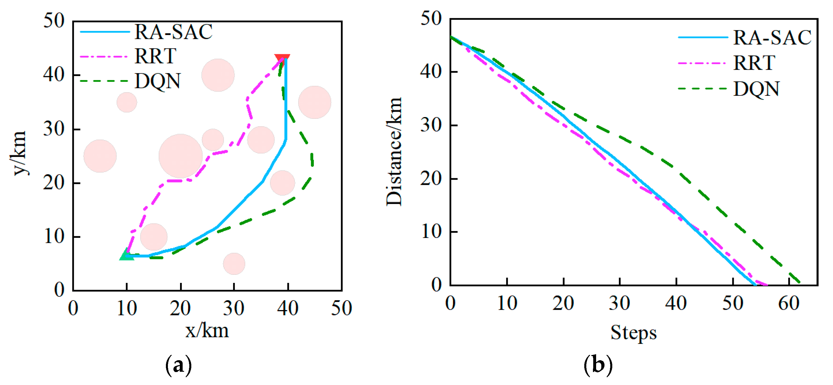
5.3.2. Scenario 2

Compared with Scenario 1, Scenario 2 increases the complexity of the environment by setting 10 obstacles with start and target point coordinates of (10, 6.5) and (39, 43), respectively. The three methods were tested under the same experimental conditions, and the results are presented in Figure 5. The planned paths of the three methods fell into different regions. When facing the first obstacle, RRT chose to find its path in the positive direction of the y-axis, while RA-SAC and DQN found their paths in the positive direction of the x-axis. Resembling Scenario 1, RRT was faster than the deep reinforcement learning methods in approaching the target in the early stage of path planning, but the path had more turning points and was closer to the obstacle boundary.

When facing the second obstacle, RA-SAC and DQN used different strategies to navigate the ship around obstacles. In the later stages of path planning, RA-SAC outperformed DQN significantly, suggesting that RA-SAC can effectively achieve a balance between risk assessment rewards and potential rewards of distance and angle. When the number of steps was 42, the path planned by RA-SAC approached the target more quickly than RRT. The ship’s approach to the target was expedited by the reward function while considering the constraints of the path turning angles in the action space, thereby facilitating smoother and more efficient path planning.

To eliminate contingency, 10 experiments were conducted using the RA-SAC, RRT, and DQN methods in the same scenario. The comparison results are shown in

Table 2. Comparison of results of repeated experiments.

Algorithm	Scenario 1		Scenario 2
	Average Path Length/km	Sum of Average Turning Angles/rad	Average Path Length/km	Sum of Average Turning Angles/rad
RA-SAC	42.07	1.65	54.53	1.68
RRT	49.71	26.21	58.20	29.38
DQN	50.74	6.96	63.59	9.11

, and each index is averaged. Compared to RRT and DQN, RA-SAC showed performance improvement, as evidenced by the minimum path length achieved and the sum of average turning angles. RA-SAC and DQN outperformed the RRT algorithm in the evaluation of the turning angle and this index, which indicates that the smoothness of the paths planned by the deep reinforcement learning method was better. The smaller the turn of the ship, the safer it is and the more fuel it saves. Simultaneously, RA-SAC had the smallest polar deviation, which means its stability was the best.

5.3.3. Experiments on Model Generalizability

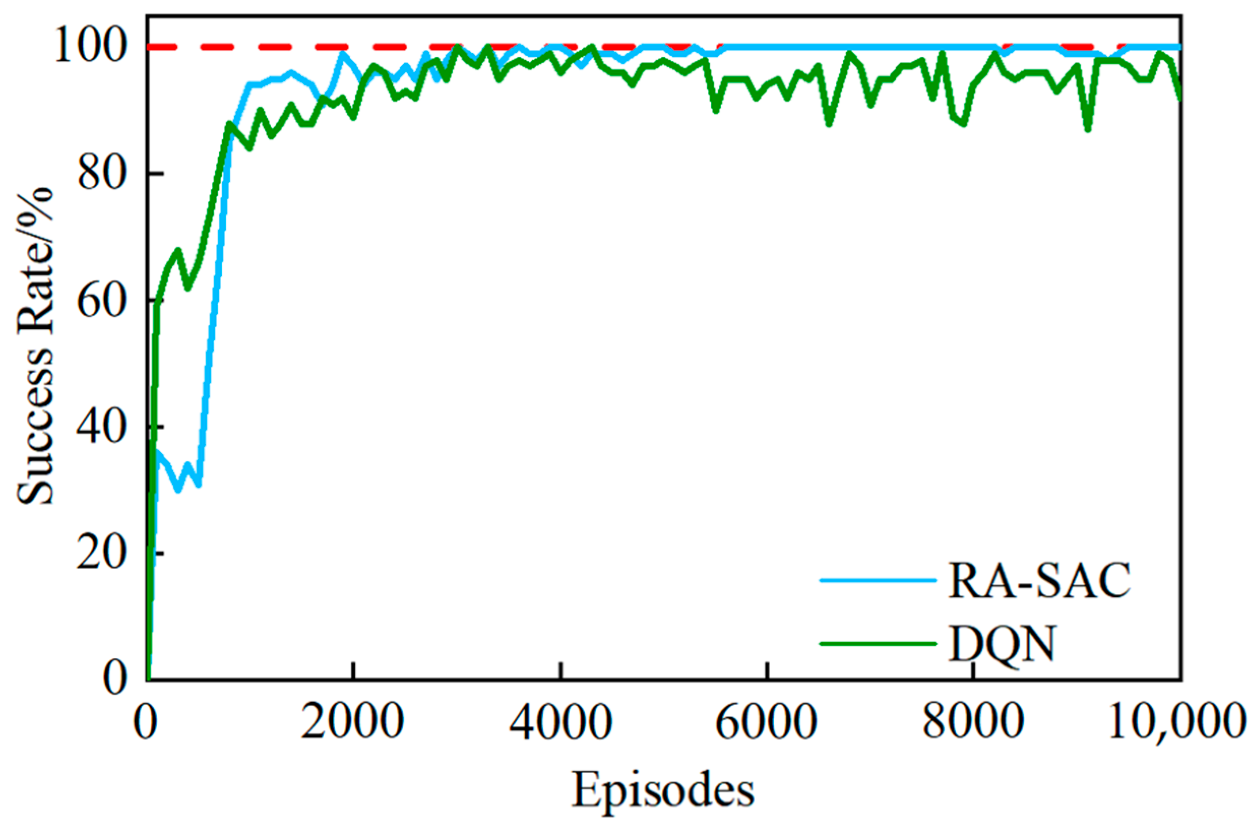
To validate the generalization and robustness of the model, a random start point and a random target point were set to train the algorithm. The random values of the position coordinates of the start and target points were treated as dynamic changes in the model inputs. Due to the randomness of the start point and the target point, different combinations of the start point and target point corresponded to different optimal trajectories and, hence, different return values. Thus, the planning success rate was used as an index to evaluate the generalization and robustness of the algorithm. The proportion of ships arriving at a random target point from a random start point and avoiding restricted navigation areas in every 100 experiments was taken as the success rate, and a higher success rate indicated better robustness of the model.

The curve of the success rate changing with the number of iterations is shown in Figure 6, which shows that in the early stage, the success rates of both methods of training tended to increase with the number of iterations, and it can be observed that the performance of DQN improved more rapidly. However, when the number of iterations reached 900, the success rate of RA-SAC exceeded that of DQN, and the curve converged more quickly. In the later stage of training, the curve was smoother and the success rate was close to 100%, indicating that the performance of RA-SAC was more stable.

The results of the generalization experiments with the algorithm are shown in

Table 3. Results of generalizability experiments.

Algorithm	Success Rate	Range of Success Rate
RA-SAC	99.56%	3.00%
DQN	95.77%	13.00%

. The total success rate represents the proportion of the ship completing the path-planning task after convergence, and the range of success rates represents the difference between the maximum success rate and the minimum success rate, which characterizes the robustness of the model. The total success rate of the paths obtained by the RA-SAC solution was 99.56%, which is an improvement of 3.96% compared with DQN; the range of the success rate after convergence of the algorithm was 3%, which is smaller than that of DQN, indicating that the generalization and robustness of the model are better than that of DQN. This is because SAC is based on maximum entropy deep reinforcement learning, which adds an entropy regularization term to the objective and is more exploratory compared to DQN, so the subsequent policy learning is faster and the performance with the policy network is more stable.

6. Conclusions

In this paper, a deep reinforcement learning-based RA-SAC path-planning method is proposed for the ship path-planning problem, considering the collision risk during ship navigation. The main conclusions are as follows:

(1)

The ship path-planning problem was modeled based on a Markov decision process and was combined with the limitations of the ship’s course to improve action space. Based on the distance and bearing data of restricted navigation areas obtained from the restricted navigation area information detection strategy, a continuous state space was constructed to improve the convergence speed and model generalization of the algorithm.

(2)

This paper proposes a path-planning algorithm that integrates SAC and navigation risk assessment. It improves sparse rewards based on the risk assessment model by introducing risk penalties to improve path safety. It also introduces distance potential rewards and angle potential rewards to effectively guide the ship to the target while avoiding restricted navigation areas.

(3)

The effectiveness of the algorithm was verified through simulation experiments, which were measured with the indicator of the path length and the sum of the turning angle. Compared with RRT and DQN, the RA-SAC algorithm showed a superior performance in scenarios of two levels of complexity. Under the environment setting of random start and target points, the success rate of the RA-SAC algorithm path planning was 99.56%, 3.96% higher than that of DQN, indicating that the model has good generalization and robustness.

This study realizes ship path-planning in a continuous environment by using the maximum entropy deep reinforcement learning method SAC, which is combined with a risk assessment model to improve the state space and reward function, and considers the limitations of the ship course to ensure smoother paths. Therefore, the planned path is both safe and economical, and the learned strategy gains a degree of generality due to the experience replay mechanism. Given the complexity of the ship’s actual navigation environment, additional uncertainties like weather, currents, wind, and waves can be taken into account in future research.