An Economic Cost/Benefit Tool to Assess Bee Pollinator Conservation, Pollination Strategies, and Sustainable Policies: A Lowbush Blueberry Case Study

Abstract

Lowbush blueberry is a mass-flowering plant species complex that grows in both unmanaged wild landscapes and managed agricultural fields in northeastern regions of both the USA and Canada. During pollination, more than 120 native bee species are associated with lowbush blueberry ecosystems in Maine, USA, in addition to three commercially managed bees. Over a 29-year period, we sampled 209 lowbush blueberry fields using quadrat and transect sampling, recording both native bee and honey bee densities, honey bee hive stocking density, and native bees as a proportion of total bees. These data were used to simulate economic uncertainty in pollination. We developed a novel algorithm, the Economic Pollinator Level (EPL), to estimate bee densities that economically warrant pollination investments such as rented hives and planting bee pastures. Statistical modeling indicated both native bee and honey bee activity density predicted proportion fruit set in fields. Honey bee activity density was well predicted by hive stocking density. Proportion fruit set adequately predicted yield. EPL was most sensitive to fruit set/m²/bee and less dependent on berry weight, rented hive stocking density, hive rental cost, lowbush blueberry price, and the annual cost of planting/maintaining pollinator pastures. EPL can be used to sustainably balance economical pollination investments/decisions with bee conservation in lowbush blueberry crops and potentially other pollinator-dependent crops.

1. Introduction

1.1. Bee Pollinator Decline—A Significant Concern

More than a decade ago, concern about the population decline of native bees and honey bees was brought to public attention globally. This drop in bee numbers is currently a major phenomenon affecting bee communities and subsequently, pollination worldwide [1,2,3,4,5]. Population decline is occurring in both managed bees such as the Western Honey Bee and many species of native wild bees. A review of the literature suggests that bee population decline is due to a lot of interacting factors such as an increase in incidence and/or virulence of bee diseases due to pathogens and parasites, climate change, pesticide exposure, low genetic diversity, limited access to forage plant resources due to declines in flowering landscapes, and altered plant–pollinator networks [3,4,5,6,7,8,9].

Some bee population decline is characterized by species extirpations, both local and regional [4,5,10,11,12,13,14,15]; although, regional extinctions have been difficult to document [16]. More commonly, there are reductions in the abundance of individual bees from a given species within a locale or sometimes over a broad geographic region [4,5,7,10,11,14]. Even the decline in abundance is difficult to prove due to the long-term oscillatory cycles that characterize the population dynamics of most bee species [17]. However, most bee experts consider the decline of bee communities a worldwide phenomenon that has been occurring over the past three to four decades [3,8,12,13,15]. This has been accompanied by concern regarding the productivity of both agricultural and natural ecosystems [18,19].

1.2. Economics of Pollination—Not Thoroughly Studied

Given the concern over both commercially managed and wild bee population declines, several studies have estimated the economic value of both bees and the ecosystem service value of bee pollination [20,21,22,23,24,25,26]. These studies suggest that the economic value of bees as pollinators often makes them the most significant input (either as a capital investment or a natural resource) in production of bee-pollinated crops. As an example, in lowbush blueberry, Asare et al. [26] found that honey bees can be the single most costly production input. In addition, they estimated that if honey bee rental prices increase by three-fold, high-input conventional production systems will break even with the currently less profitable low-input conventional production systems.

Assessment of the economic value of pollinators is challenging because often there is a mixture of native wild bees along with commercially managed bees, such as honey bees and bumble bees. This is the case in the two bee-pollinated native crops in northeastern North America, lowbush blueberry and cranberry [26,27]. In our study system, lowbush blueberry, native wild bees are more efficient than honey bees [26]. A per bee density increase in native wild bees results in an increase in fruit set of 14.9%, whereas a per bee increase in honey bee density during bloom will result in a 6.1% increase in fruit set. However, because honey bees are rented by blueberry growers, their numbers can be increased easily by increasing the capital outlay for pollination in a given year. In Maine lowbush blueberry, Hoshide et al. [27] found that the attributable net income for native wild bees is USD 613/ha, and for honey bees it is USD 913/ha. These authors [27] also found that for cranberry growers in Massachusetts, the attributable net income for native wild bees is USD 689/ha, and for honey bees it is USD 1320/ha. Consumers of bee-pollinated produce also affect the economics of bee-pollinated crops and are willing to pay 6.7 times more than growers for native bee-pollinated cranberries. This is similar to a finding of consumer willingness to pay for blueberries [27].

Therefore, the economics of bee pollination is dependent upon individual crops, mixtures of bee pollinator species in those crops, and the consumers that buy foods produced from these crops. Some studies have focused on how to evaluate this economic metric, as well as strategies that can be implemented to increase agricultural crop resilience and robustness given trends of declining bee numbers [27,28,29,30,31,32,33,34,35,36,37,38,39]. These strategies involve planting flowering plant reservoirs, minimizing pesticide exposure to bees by relying on insect pest management for crop protection, conserving bee habitat as non-fragmented areas, constructing and/or protecting existing nesting habitat for bees, and reducing transmission of bee diseases by limiting commercial production and use of exotic pollinators.

1.3. Sustainable Pollinator or Pollination Protection Policies—A Global Perspective

Along with the development of economic values of bees and their ecosystem service of pollination, policies have been formulated to protect this economically valuable resource and halt or even reverse the decline in both wild native bee and commercially managed bee populations, such as the honey bee. Senapathi et al. [40] formulate a debate that should be heeded. The authors suggest that before policy is formulated, it is important to determine if policy should address conserving bee diversity or maintaining the ecosystem service of pollination. They argue that the policies for each of these objectives may not be the same. Because the ecosystem service of pollination is dependent upon conservation of species diversity in all habitats, policies seeking to conserve bee biodiversity should focus on both managed agricultural and natural habitats.

The development of public policies to prevent declines in both bee populations and pollination is complex and needs participation by multiple stake holders and experts, in addition to educated government legislatures and regulators [41,42]. These policies also should be designed to work on multiple scales: spatial, temporal, actor (stake holders), social, and sector scales [43], with the involvement of beekeepers as policy formulators [44]. Additionally, urban landscapes are often ignored as bee habitats, and should be included in public policy for conserving bee diversity [45]. From a global perspective, another forgotten sector tends to be developing countries, which are often left out of policy think tanks [46,47]. Successfully enhancing pollination security globally can address three out of seventeen of the United Nation’s Sustainable Development Goals, namely ensuring responsible consumption and production (Goal #12). This can balance decent work and economic growth (Goal #8) in farming communities, while better conserving life on the land (Goal #15) found in pollinator habitats [48].

Much discussion and policy formulation on conservation of bee biodiversity has occurred in the European Union (EU) [49,50,51,52,53,54]. These policies are usually designed for conservation over a large geographic area, often involving habitat conservation, protection of wild bees on farms, reduction in pesticide use through farm adoption of integrated pest management, banning of highly toxic pesticides, city planning, support of organic agriculture, research on apicultural practices, enhancing crop diversity on farms, and improving public awareness, just to name a few strategies. The United States of America (USA) has a much more incentive-driven approach with government programs that subsidize both farmers for establishing pollinator plantings and state municipalities for establishing roadside floral resource plantings, pesticide certification programs, and apiary programs [55,56].

Federal programs in the USA also fund research and demonstration projects conserving bee diversity [41,56]. Between 2000 and 2017, 109 USA state policy laws were developed and written for pollinator conservation [57]. The objectives of these policies were to conserve bee habitat, provide integrated pest management in order to minimize the impact of pesticides on pollinators, monitor bees, move at-risk commercial pollinators from stressful environments, enhance pollination, improve pesticide standards, increase critical research funding, and to improve public awareness of pollinators [42]. The strategies supported and developed into policy objectives are similar for both the USA and the EU. Another focal area when structuring policy is agricultural landscapes [49,52,53]. The advantage of this approach is that many agricultural landscapes are concentrated within geographic regions and are imbedded in specifically managed and natural ecosystems that are characterized by unique regional pollinator complexes and specific stressors that might be impacting the pollinator communities. Threats to pollinator communities may be well defined, and thus can be more easily addressed with specific regional strategies. This approach has been taken in our study of the Maine lowbush blueberry agroecosystem, where it is critical to understand if the increase in lowbush blueberry yield and revenues from using particular pollination strategies warrants the cost of investing in these strategies, using economic risk analysis.

1.4. Lowbush Blueberry—A Unique Native North American Wild Crop

A brief description of the lowbush blueberry cropping system is described here to provide background for those not familiar with this regional cropping system. Yarborough [58] has written a detailed description of lowbush blueberry production and the overall industry which we have summarized. Lowbush blueberry describes several North American native ericaceous plants in the genus Vaccinium, the most abundant being the sweet lowbush blueberry, Vaccinium angustifolium Aiton. The crop has not been improved through breeding and it is not planted. Lowbush blueberry plants are natural understory plants in the Acadian and Boreal forests in Maine, Quebec, and the Canadian Maritime provinces. To initiate a field, a forest is clear-cut harvested and the understory blueberry plants are released from plant competition by periodic burning or the application of selective herbicides. Once established, fields are usually managed on a biennial cycle, the first year of a two-year cycle is characterized by pruning through burning or mowing. In this first year, the plants grow vegetatively and produce flower buds. During the second year, the plants bloom. After being pollinated mostly by bees, the plants produce fruit that is harvested at the end of the summer. In the fall of this second year or during the spring of the following year, the field is pruned again. Growers rely upon the native bee community for pollination, but many producers supplement the native bee community with managed bees, mostly honey bees, but sometimes commercially produced bumble bees (Bombus impatiens Cresson). For more details about this native North American cropping system and its pollination ecology and requirements, please see Bushmann and Drummond [59].

1.5. Goals and Objectives for Lowbush Blueberry Sustainable Pollination

We have been studying the bee community and pollination in Maine for more than 30 years, since before 1992 (see [59] for references). Between 1993 and 2021, we sampled 209 commercial lowbush blueberry fields and quantified the relative densities of managed (Western Honey Bee) and native wild pollinators, as well as lowbush blueberry fruit set and yield. Bee sampling methods have been developed, as well as both farm field-level and landscape-level tools for bee conservation and pollination decision making. In this study, we summarize the data collected during our farm surveys over a 29-year period.

Using these data, our goal was to conduct a risk assessment of the economics of pollination in Maine lowbush blueberry along with the development of a tool that can be used by growers, pollination researchers, economists, and policy makers to assess the viability and robustness of novel pollination tactics. Our objectives are as follows:

(1)

Determine that both native bees and managed honey bees contribute, in part, to fruit set;

(2)

Determine the relationship between honey bee hive stocking density and honey bee forager populations in the field;

(3)

Estimate the relationship between fruit set and yield;

(4)

Propose, formulate, and use an “Economic Pollinator Level” (EPL) metric for evaluating future conservation and pollination policies and strategies using case study examples;

(5)

Conduct Monte Carlo simulations on the economic uncertainty or risk in lowbush blueberry pollination by way of using the EPL to test pollination tactics.

Change is occurring at a rapid rate in global markets, climate, pollinator community diversity, and abundance. These changes are already beginning to impact lowbush blueberry production and economics. One of the critical inputs to the existence of lowbush blueberry production is the continued sustainability of pollination. Long-term data of the impact of pollinators on crop fruit set and yield, as well as metrics such as the EPL, can be used help producers focus their limited resources more efficiently to optimize the impacts of pollination strategies. This is extremely important, specifically in light of how climate change may alter pollinator community diversity and abundance, as well as the yields and economics of lowbush blueberry production, as is occurring in other cropping systems.

2. Materials and Methods

2.1. Lowbush Blueberry Sites Sampled

Two hundred and nine commercial lowbush blueberry fields were sampled between 1993 and 2021 (more details regarding these sites can be found in [26,31,59]). These fields were located in the major lowbush blueberry growing regions in Hancock, Knox, Penobscot, Sagadahoc, Waldo, and Washington counties in Maine, USA. In each field during bloom, bee densities and fruit set were assessed. Prior to harvest, yield was estimated either by manually raking or obtaining yield estimates from cooperating growers.

Bee sampling in these 209 fields measured bee population activity densities expressed as bees/m²/min. This metric of bee density was estimated for each field two to three times during lowbush blueberry floral bloom. At each sample date from 1993 to 2021, 10–20 m² quadrats of blooming crop were arbitrarily selected. Each sampled quadrat represented 10–20 clones, where each clone is a unique plant. For 1 min, the number of honey bees (Western Honey Bee, Apis mellifera (L.)) and wild native bees foraging on the lowbush blueberry bloom were counted and recorded. Bee abundance for each of the 10–20 m² sampling quadrats was averaged for each visit and over all the visits for each field.

In 1993, for the first sampling period, five to seven 100 m by 1 m belt transects were used to estimate native bee and honey bee relative density. Bees were counted and the time taken to survey the transect length was recorded. The abundance of bees from these transects were converted to bees/m²/min, so that they could be averaged with square quadrat counts. Both quadrat and belt transect sampling of bee abundance were only conducted between 0900 and 1500 h and when the weather was at least partly sunny and warmer than 10 °C, with average wind speed of less than 30 km/hr.

Bees were only identified as honey bees or wild native bees, although separate hand collections and bowl trapping enabled species to be identified by family and species [26,31,59,60]. There are over 90 species of wild native bees associated with lowbush blueberry [59,60] ranging from 5 to 42 species per field [58]. The relative abundances of the major bee taxa groups found in Maine lowbush blueberry fields during this study are bumble bee (Bombus spp.) queens (8–22%), digger bees or Andrenidae (15–45%), sweat bees or Halictidae (12–24%), leafcutting and mason bees or Megachilidae (2–5%), and cellophane or yellow-faced bees or Colletidae (1–3%) [26,59]. During bee sampling, the number and stocking density (hives/hectare) of honey bee hives in a field were recorded.

Fruit set was estimated during bloom in the same 209 fields that bee relative density was measured. In early- to mid-May of each year, six to nine representative clones (genetically distinct plants) were selected in each field. Clones typically range in size from <1 m² to >500 m², with a mean of 43.3 m² [61]. Two to three clones were selected near the field center, two to three about halfway between the edge and center, and two to three near the field edge. To compensate for micro-regional growth differences, clones were selected throughout the field. Clones were not selected directly near honey bee hives.

Four to six stems were arbitrarily chosen and tagged for each clone. Stems were visited two to three times. The first visit involved a count and recording of the number of flowers per stem. A second visit, in early June, involved counting and recording set fruit as a measure of fruit set, which we refer to as early fruit set. In late June, a final count of developing fruit was conducted and recorded. The proportion of fruit at the final count that developed from the initial flowers is a measure of late fruit set, after some of the premature fruit drop has occurred. Late fruit set is a good measure of pollination intensity, but not necessarily a measure of harvestable fruit as harvest typically occurs 3 to 6 weeks later, a time period during which environmental conditions can further reduce fruit number. In all cases, the proportion fruit set/stem was calculated, and the stem estimates were averaged to provide a clone estimate of proportion fruit set. Clone estimates were subsequently averaged to provide a field-level estimate of proportion fruit set.

Yields were obtained from the same fields in which bee density and fruit set were measured. Most yields were obtained from lowbush blueberry producers immediately after harvest. In 1993, a few fields were sampled with a hand rake using ten 1 m² quadrats or using two to three 10 m² quadrats. All yields were converted to kilograms of fruit harvested per hectare. Yields were obtained for 199 of the 209 fields sampled.

2.2. Statistical, Theoretical, and Monte Carlo Analyses

All statistical and probability modeling was conducted using the statistical software JMP Pro version 17 [62]. Economic Monte Carlo simulations were conducted using the @Risk software version 7.6 from Palisade [63]. Monte Carlo simulations compared different pollination systems (e.g., honey bee versus native bee pollination for lowbush blueberries in Maine) by contrasting the distribution of outcomes of an agricultural metric (e.g., EPL) and determining factor(s) that have a great impact on outcomes such as input quantities and prices [64].

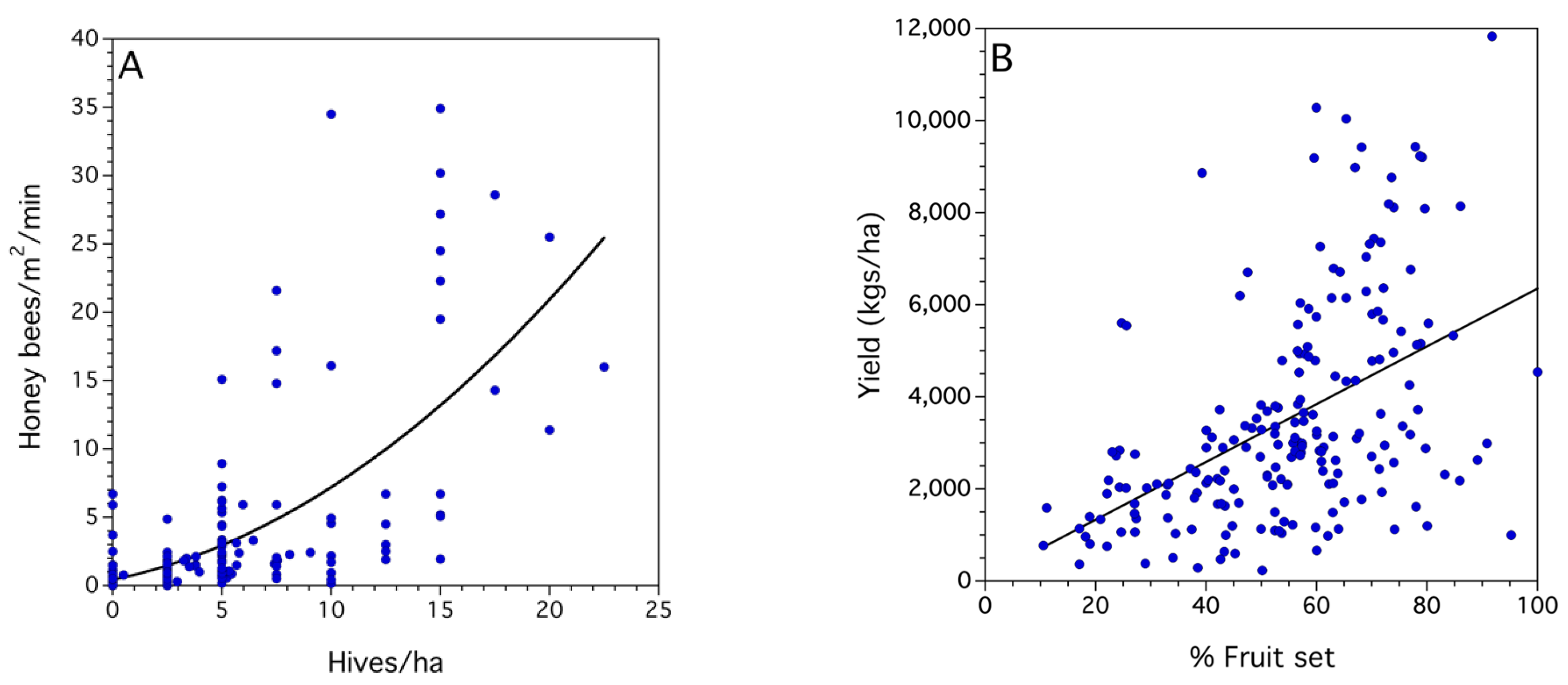
2.2.1. Modeling Relationships between Bee Activity Density, Hive Stocking Density, Proportion Fruit Set, and Yield

General mixed linear models were used to estimate bee-to-bee and bee-to-pollination relationships. Use of these models can directly model correlations between and within predictors, account for unbalanced designs, and often does not require transformations upon the dependent variable [65]. These models have also been shown to have power in complex systems with much noise and interacting factors, such as field and pollination ecology [66]. Random effects were study and year within study. A study represents a series of years in which fields were sampled for a specific project. The data consisted of 209 fields sampled over 29 years, represented by 4 studies. The fixed effects were the hypothesized causal or predictor variables of interest. Fixed effects were tested with the Satterthwaite adjusted error degrees of freedom [62]. Random effects were tested with the Wald test [62]. The coefficient of determination calculated was the conditional r². These models were used to determine that the fixed effects or predictors do indeed determine the average trend in the dependent variable. They were not used to predict individual year data in fruit set or yield.

Least squares linear regression [62] was used to determine the relationship between grower investment in rental of honey bee hives on a per hectare basis and the monetary value of the blueberry crop yield (kg/ha). The cost of renting hives was set at USD 100/hive and the value of the harvested berries was set at USD 2.50/kg blueberries. Both values are on the high end of costs and values witnessed by one of the authors (F.A. Drummond) over the past two decades. The cost of hives was square root transformed so that the pattern of residuals was homogeneously distributed. Another regression model was constructed to determine the relationship between honey bee stocking density (hives/ha) and the ratio of blueberry crop value (USD) to the dollar value (USD) invested in honey bee hives by growers. The honey bee hive stocking density was transformed to the power of stocking density (X^a) in order to improve the pattern of residuals around the regression line.

To estimate long-term trends in relative abundance of native bees in lowbush blueberry fields from 1992 to 2021, a least squares linear regression was compared to a smooth spline fit of the square root transformed native bee activity density. In both models, we used the square root transformation of the data to construct a data set that demonstrated homogeneity of variance and a reduction in temporal autocorrelation (r_t = 0.367, p < 0.05) across the time series. Because we did not sample bee activity density in every year and there were several years with missing data, time series analysis was not used for modeling these data [67].

2.2.2. Development of an Economic Pollinator Level

The economic threshold for pest decision making was developed by Stern et al. [68]. These authors conceptualized the economic threshold as “The lowest population density of a pest that will cause economic damage; or the amount of pest injury which will justify the cost of control”. With pollinators, one could also ask the question, what is the bee population or community-level activity density that will increase economic gain such that this gain justifies the cost of pollination management. Pollination management costs can include the rental fee paid for importing honey bee or bumble bee hives to a farm, the cost of establishing pollinator reservoirs (plantings) to enhance forage and build up native bee community densities, the cost of least toxic pesticides to conserve native bee numbers, or the cost of providing nests or nest habitat for soil- or twig-nesting bees.

The economic injury level, a term first proposed by Pedigo et al. [69] defines a threshold that provides a buffer. It is the pest level where the cost of pest control is greater than its benefits. This is lower than the economic threshold or “action threshold” where the benefits of control are greater than its cost.

The simplest model of the economic injury level is represented in Equation (1):

$$\mathrm{EIL}=\frac{\mathrm{C}}{\left(\mathrm{V}\times \mathrm{L}\right)}$$

(1)

where C is the cost of pest control, V is the monetary value of the crop per unit measure, and L is the monetary value of the loss due to an individual pest per unit measure. In a similar manner we can design an operational model for the “Economic Pollinator Level” or EPL. One formulation of the model is Equation (2):

$$\mathrm{EPL}=\frac{\mathrm{C}}{\left(\mathrm{V}\times \mathrm{P}\times \mathrm{B}\right)}$$

(2)

where C is the monetary cost of pollination management on a per m² or per hectare unit basis; V is the monetary crop value per unit (for example, per kg of fruit); P is the number of flowers set by an “individual bee” during bloom that will become harvestable fruit; and B is the weight of a single set flower as a fruit, the unit of benefit from pollination.

The monetary value of C can be actual dollars that are spent either renting hives or planting bee forage, discounted on an annual basis. The value of C can also be the intrinsic conservation value of wild native bees. Arriving at the monetary crop value is fairly straight-forward. It can be a forecasted value for the future or derived from the previous year or a past long-term average.

The next two variables, P and B, are more difficult to estimate and averages or “back of the envelope estimates” might be the best and only measure available for such a complicated system as crop pollination. The number of flowers set (P) by an individual bee is generally dependent upon bee species in the lowbush blueberry system. In the laboratory, Javorek et al. [70] show that honey bees are much less efficient than several species of wild native bees in placing pollen tetrads on lowbush blueberry stigma. This has been confirmed in the field by Asare et al. [26]. In one of the following examples, we use an average for “native bees.” An average can also be obtained for a commercial bee such as the Western Honey Bee. If one assumes independence and no co-linearity among bee activity density predictors, then the slope coefficient (b) from estimating a linear relationship between bee activity density (D_ba) and proportion fruit set (FS_p) can be used, where the intercept (a) is the FS_p without any bees. Here, the default value for D_ba = 1, prior to adjustment by b:

FS_p = a + b(D_ba)

(3)

Depending upon the crop, one needs to assume or have previously determined the proportion of set flowers that results in a known number of harvestable and marketable fruit [71]. So in essence, fruit set is used as a proxy for harvestable fruit. This is usually a more direct estimate of harvestable fruit than an indirect relationship between pollinator density and marketable yield due to weather stress conditions, pests and weed competition, and various harvesting and packing losses.

The last variable, B, is highly consistent and standard for some fruit, but for other fruit it may be quite variable. Lowbush blueberry fruit mass is dependent upon plant genotype, soil moisture, air temperature, soil fertility, pollination efficacy (number of ovules fertilized), compensatory growth as a function of fruit density per stem due to fruit drop, and/or pest attack. In the case studies presented in the results section, we used the average mass of 0.4 g per single berry for harvested ripe lowbush blueberries [60,61].

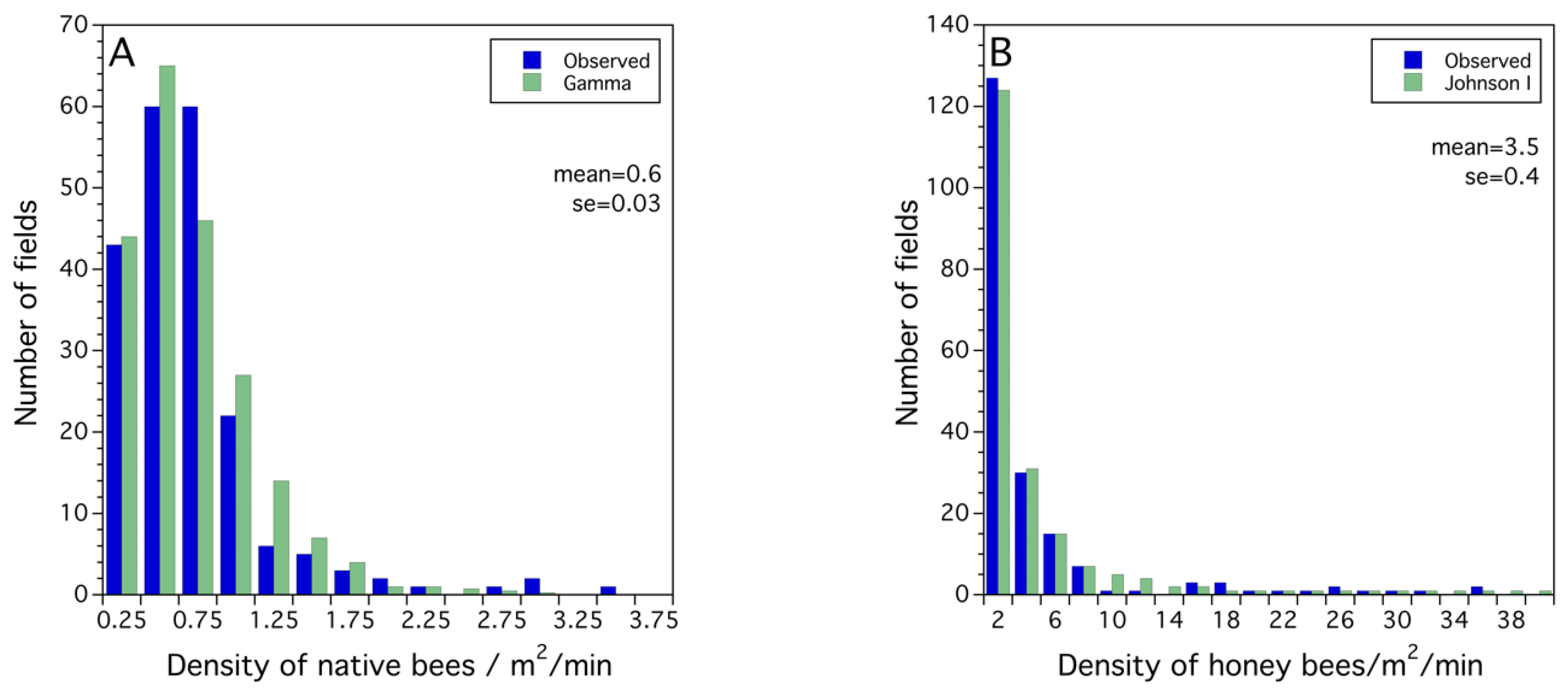
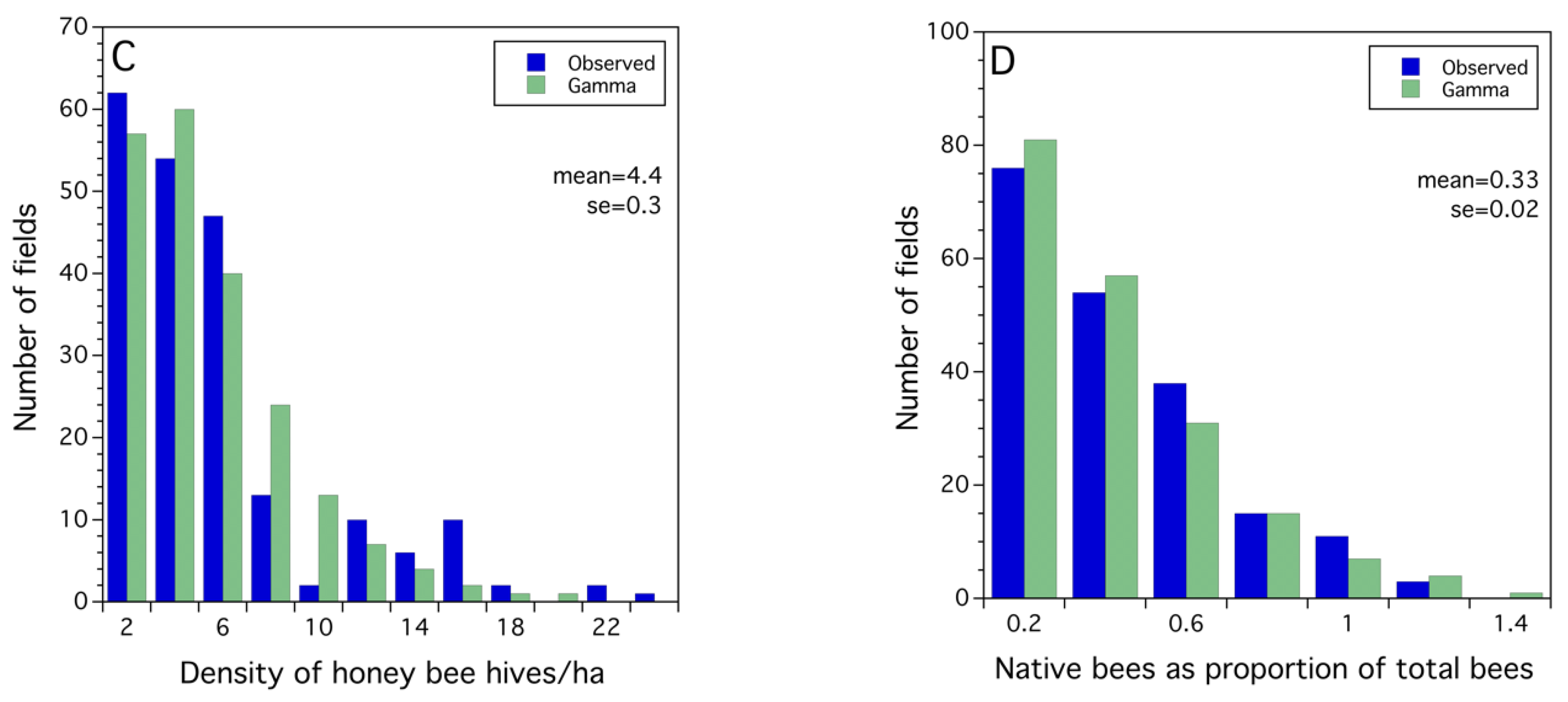
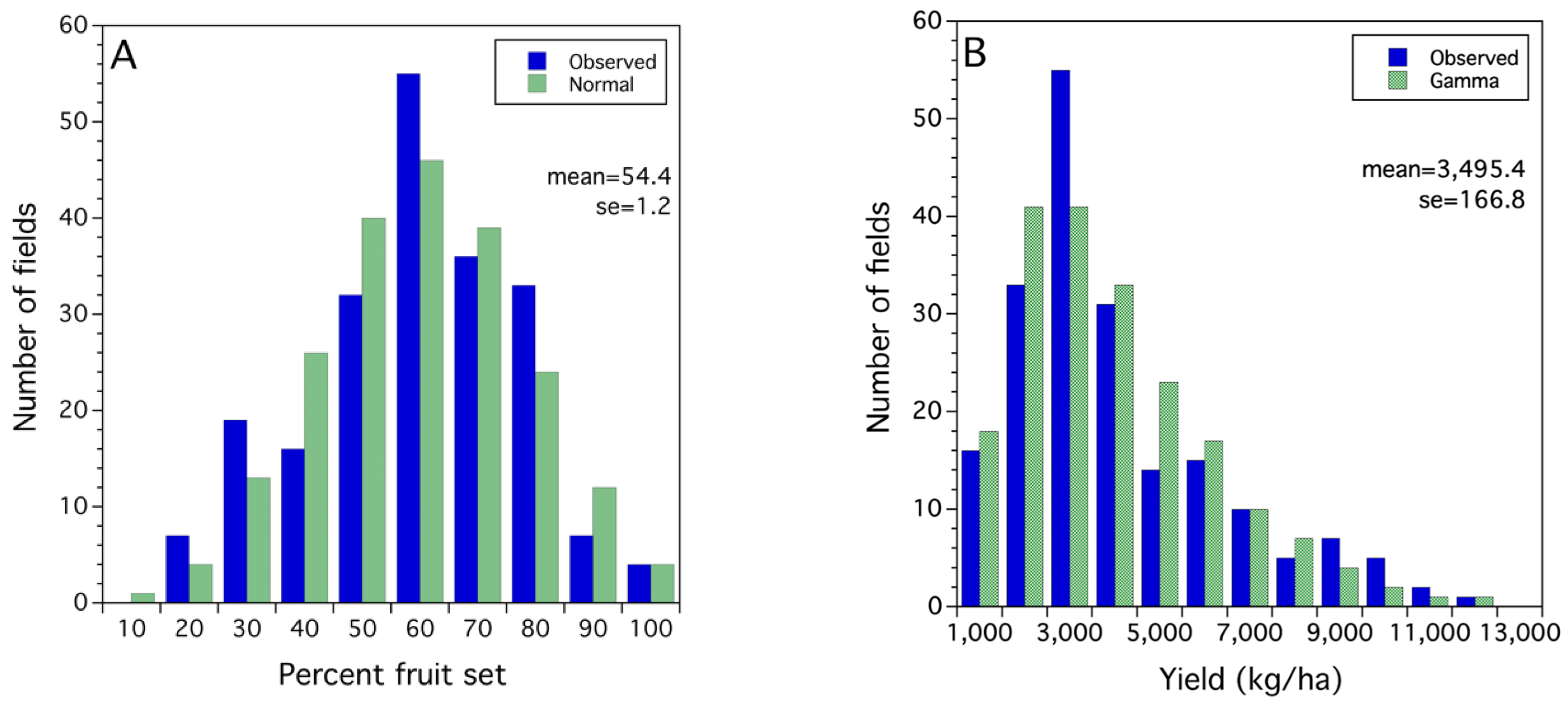
2.2.3. Probability Modeling—Fitting Probability Density Functions to Observed Frequency Distributions

Probability density functions were used for input by the Monte Carlo software, @Risk version 7.6 (Palisades software). Frequency distributions of six measures recorded in each field were constructed: (1) the observed activity density of native wild bees (bees/m²/min/field), (2) activity density of honey bees (bees/m²/min/field), (3) proportion of native bees (native bees/total bees) per field, (4) honey bee hive stocking density (hives/ha) per field, (5) mean proportion fruit set/field, and (6) yield (kilograms of berries/ha/field). A diversity of probability density functions were fit to and selected as models for the observed frequency distributions, when goodness of fit tests provided evidence that there was no significant difference (p > 0.05) between observed and model frequency distributions. The goodness of fit tests utilized were the Cramer–von Mises W test, Shapiro–Wilk W test, Kolmogorov D test, and Anderson–Darling test [62], depending upon the probability density function being evaluated. Probability modeling was conducted with JMP [62].

2.2.4. Monte Carlo Simulation of Economic Uncertainty or Risk of Lowbush Blueberry Pollination and Yield

Economic uncertainty or risk of the Economic Pollinator Level (EPL) for both honey bees and native bees can be modeled by stochastically changing key variables used to calculate EPL when there is historical time series data available for these variables. This Monte Carlo approach to assessing economic pollination risk determines not only the probability distributions of EPL outcomes, but also the sensitivity of EPL to specific variables (for sensitivity analysis in lowbush blueberry, see [61]). Tornado diagrams can be generated that indicate this sensitivity of the EPL to various impact factors or the range of the EPL given stochastic variation in each variable. The largest range of variable variation is at the top of the tornado diagram followed by ranges that become narrower toward the bottom of the diagram [63]. The variables with the largest EPL range denote those variables to which the EPL is most sensitive.

Variables used to calculate EPL for honey bees and native bees that had available times series data included the monetary cost of pollination (C), the value (V) of lowbush blueberries (USD/kg) in Maine, the number of flowers set per m² per bee (P), and B which is the weight of one marketable individual lowbush blueberry in kg (equation 2). In order to run stochastic Monte Carlo simulations in @Risk [63], historical data for C, V, P, and B were fitted to functional forms for probability distributions (Table 1). The values of C and V were calculated in U.S. dollars (USD).

For Monte Carlo simulations of EPL, the variable C for native bees was based on pollinator pasture cost budgets developed for the University of New Hampshire (UNH) in 2016 (see Appendix A,

Table A1. Native bee pasture budget for Maine, USA, lowbush blueberries with costs in USD.

Annual Pollination Pasture Budget	Scale:	0.067	Hectares	5.953	Year Stand Life
Characteristic/Costs	Total		Per Hectare		Per Square Meter
Number of Acres of Pasture	0.164		-		-
Number of Hectares of Pasture	0.067		-		-
Annual Operating Expenses (USD)
Lime	0		0		0
Seedlings	0		0		0
Seeds	77		1160.28		0.116
Seed Amendments	12		184.49		0.018
Labor
Establishment Year 1	50		745.30		0.075
Ensure Establishment Years 1 to 3	8		114.74		0.011
Annual	41		614.72		0.061
Diesel Fuel
Establishment Year 1	10		147.52		0.015
Ensure Establishment Years 1 to 3	0.40		6.06		0.001
Annual	0		0		0
Oil	3		38.10		0.004
Maintenance and Upkeep	111		1673.65		0.167
Utilities	0		0		0
Total Operating Expenses	312		4684.86		0.468
Annual Ownership Expenses (USD)
Depreciation and Interest
Buildings and Structures	116		1746.74		0.175
Bee Pasture Equipment	120		1803.84		0.180
Repair and Management	16		239.57		0.024
Tractors and Vehicles	422		6341.48		0.634
Land	17		252.03		0.025
Interest on Loans	0		0		0
Insurance	0		0		0
Taxes	195		2930.90		0.293
Total Ownership Expenses	886		13,314.57		1.331
Total Annual Cost (USD)	1197		17,999.43		1.800

). Variable costs such as labor, fuel, and seed, as well as fixed costs such as depreciation on equipment used were stochastically varied using historical time series data for these input costs (see Appendix A, Table A1). These nominal values were then adjusted for inflation to derive real values using appropriate producer price indexes (PPI’s) from the U.S. Bureau of Labor Statistics (BLS) [72]. The PPIs are unitless indexes that track the changes in input prices exclusively due to monetary inflation over time [73].

Table 1. Data sources for Economic Pollinator Level variables used for honey bees and native bees in Maine, USA.

Economic Pollinator Level Variables	Pollination System	Years	Data Source	Producer Price Index Adjust for Inflation [73]	Function Form for Probability Distribution Fit
(1) Monetary cost of pollination (C)	Native Bee Pasture	2002–2023	Various ( Table A2. Data sources for cost line items used for native bee pasture budget for Maine, USA. Native Bee Pasture Cost Line Items Data Source(s) Years Producer Price Index Used to Adjust for Inflation [74] Function Form for Probability Distribution Fit Variable Costs   Seeds (wildflower mix) Neal 2019 [109]; OPN Seed [110]; Wong 2017 [111] 2003–2022 Hay, hayseeds and oilseeds Triangular   Vermiculite U.S. Geological Survey, National Minerals Information Center [112] 2002–2022 Nonmetallic mineral products Triangular   Labor U.S. Economic Research Service [113] 2002–2022 Already adjusted for inflation Pareto   Diesel Fuel USDA, ARS [114]; Hoshide et al., 2006 [115]; Asare et al., 2017 [26] 2002–2023 No. 2 diesel fuel Triangular   Oil Asare et al., 2017 [26] 2002–2022 Finished lubricants Uniform   Maintenance and Upkeep Adjusted in proportion to total capital used 2002–2022 Repair and maintenance services (partial) Uniform Fixed Costs   Depreciation     Equipment Storage Asare et al., 2017 [26] 2002–2022 Farm service buildings and other prefab./portable Triangular     Tiller (for tractor) University of Minnesota Extension [116] 2002–2022 Farm plows, harrows, rollers, pulverizers, etc., and attachments Uniform     Landscaping Rake Venturini et al., 2017 [31] 2002–2022 All other farm machinery Uniform     Paint bucket (seed) Venturini et al., 2017 [31] 2002–2022 All other farm machinery Uniform     Culti-Packer Venturini et al., 2017 [31] 2002–2022 Farm plows, harrows, rollers, pulverizers, etc., and attachments Uniform     Flail Mower (tractor) Asare et al., 2017 [26] 2002–2022 Farm dairy equipment, sprayers and dusters, farm blowers, and attachments Triangular     Hand Clippers Venturini et al., 2017 [31] 2002–2022 All other farm machinery Uniform     Computer Asare et al., 2017 [26] 2002–2022 Personal computers and workstations Uniform     Tractor University of Minnesota Extension [116] 2002–2022 Total tractors Triangular   Land U.S. Economic Research Service [117] 2002–2020 Already adjusted for inflation Triangular   Property Tax Maine State Government [118] 2012–2021 Not adjusted since no PPI available Triangular )	Various (Table A2)	Various (Table A2)
	Rented Honey Bees	2003–2022	Cooperating producer [26]	Lumber and plywood	Uniform
(2) Value of wild blueberries (V)
(a) Frozen	Native Bee Pasture and Rented Honey Bees	2002–2021	USDA, NASS [74]	Frozen fruits/vegis	Extreme value
(b) Freshpack	Same as above	Same	Same	Fresh blueberries	Laplace
(3) Number of flowers set per m2 per bee (P)	Native Bee Pasture and Rented Honey Bees	2005, 2013, and 2015	[26,59,61]	Not used	Gamma Gamma
(4) Lowbush blueberry single berry weight (B)	Native Bee Pasture and Rented Honey Bees	2006, 2007, and 2011	[59,61,71]	Not used	Weibull

Table 1. Data sources for Economic Pollinator Level variables used for honey bees and native bees in Maine, USA.

Economic Pollinator Level Variables	Pollination System	Years	Data Source	Producer Price Index Adjust for Inflation [73]	Function Form for Probability Distribution Fit
(1) Monetary cost of pollination (C)	Native Bee Pasture	2002–2023	Various (Table A2)	Various (Table A2)	Various (Table A2)
	Rented Honey Bees	2003–2022	Cooperating producer [26]	Lumber and plywood	Uniform
(2) Value of wild blueberries (V)
(a) Frozen	Native Bee Pasture and Rented Honey Bees	2002–2021	USDA, NASS [74]	Frozen fruits/vegis	Extreme value
(b) Freshpack	Same as above	Same	Same	Fresh blueberries	Laplace
(3) Number of flowers set per m2 per bee (P)	Native Bee Pasture and Rented Honey Bees	2005, 2013, and 2015	[26,59,61]	Not used	Gamma Gamma
(4) Lowbush blueberry single berry weight (B)	Native Bee Pasture and Rented Honey Bees	2006, 2007, and 2011	[59,61,71]	Not used	Weibull

For honey bees, the variable C equals the number of hives used per hectare multiplied by the cost per hive (USD/hive). The number of hives used per hectare was based on a past socio-demographic survey of lowbush blueberry producer practices conducted from 2012 to 2013, using honey bee stocking densities from 21 of 38 surveyed producers [26]. The cost per hive from 2003 to 2022 was provided by a cooperating lowbush blueberry producer. Costs per hive over this time period were adjusted with the PPI for lumber and plywood used to make Langstroth box hives, since BLS does not keep a PPI for rented honey bee hives [72].

The variable V for Maine lowbush blueberries (2002 to 2021) was obtained from the U.S. Department of Agriculture (USDA), National Agriculture Statistics Service (NASS) [74]. As shown in Table 1, all monetary costs and values were converted from nominal values to real (inflation adjusted) values (2022 USD) using PPI’s similar to inflation adjustments made for C for honey bees [72]. Using nominal monetary values over multiple years without adjusting for inflation can cause distortion because variation in short-term rates of inflation for agricultural inputs can be highly variable [75].

EPL for honey bees and native bees used the same data sources for stochastic simulations for both the variables P and B. Calculations for the variable P (flowers set per m²) used 388 field observations of flowers/m² for Maine lowbush blueberries collected during 2005, 2013, and 2015 in the blueberry production regions of Midcoast and Downeast Maine [26,59,61]. These observations of flowers/m² were multiplied by assumed percentages of flowers that result in set fruit for native bees (10%) and honey bees (1%) [61], and then were adjusted for the distribution of lowbush blueberry flowers that are available daily for bee visitation and thus pollination, where flowers are viable for 5 days once a flower is open [71]. The distribution of berry weight (B) relied on 714 observations from studies conducted in Downeast Maine [61,71].

The @Risk software from Palisade [63] also graphs the sensitivity of input parameters to variables (e.g., EPL, cost of pollinator pasture) using tornado diagrams. Tornado diagrams are composed of horizontal bars indicating the minimum to maximum range of values of a variable subject to stochastic changes in input parameters. The input parameter resulting in the widest range is at the top of tornado diagrams with subsequent input parameter ranges that become narrower toward the bottom of the diagram. This arrangement makes the diagram look like a tornado. Tornado diagrams were evaluated for EPL for both managed honey bee and wild native bee pollination of lowbush blueberries, as well as for the cost of installing pollinator pasture for native bees.

3. Results

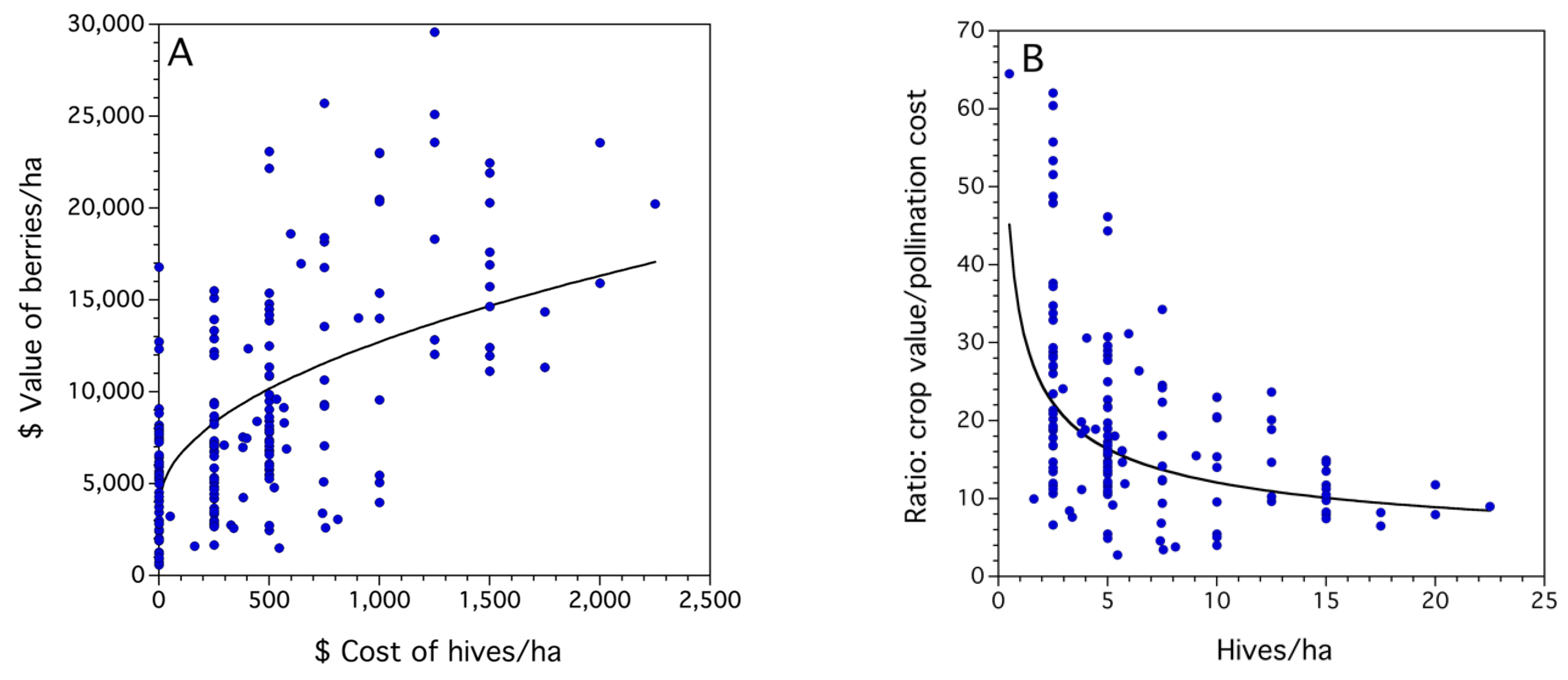
3.1. Frequency Distributions of Sampled Bee and Crop Pollination and Production Metrics

The frequency of native bee activity densities (bees/m²/minute) in lowbush blueberry (Vaccinium angustifolium Aiton) fields (n = 209) is depicted in Figure 1A. Native bees were from the genera Bombus, Andrenidae, Halictidae, Megachilidae, and Colletidae. The mean activity density was 0.57 ± 0.03 (se) bees/m²/min. This translates to 5686 ± 335 native bees/hectare (ha)/min. The range was 0 to 3.25 bees/m²/min which is 0 to 32,500 bees/ha/min. The Gamma probability density function described the observed data (Cramer–von Mises W test, W² = 0.177, p > 0.25). The parameters of the Gamma function are α = 2.065 (shape), σ = 0.275 (scale), and θ = 0.0 (threshold parameter).

The frequency of honey bee (Apis mellifera (L.)) activity densities between fields (n = 209, not all fields had hives deployed) is depicted in Figure 1B. The mean activity density was 3.46 ± 0.45 bees/m²/min. This translates to 34,600 native bees/ha/min. The range was 0 to 34.85 bees/m²/min, equivalent to 0 to 348,500 bees/hectare/min. The Johnson SL probability density function fit the observed data well (Shapiro–Wilk W test, W = 0.989, p = 0.172). The Johnson SL function parameters are γ = −0.165 (shape), δ = 0.691 (dispersion), θ = −0.027 (location), and σ = 1.000 (scale parameter). Both native bee and honey bee distributions are highly skewed, with the distribution for honey bees being more skewed than that for native bees (Fisher’s G1 statistic, HB = 3.18, NB = 2.71).

The frequency of honey bee hives/ha between fields (n = 209) is depicted in Figure 1C. The mean hive density was 4.40 ± 0.32 hives/ha. The range was 0 to 22.5 hives/ha. The Gamma probability density function marginally fit the observed data but was the best probability density function describing the observed frequency distribution (Cramer–von Mises W test, W² = 0.263, p = 0.08). The parameters of the Gamma function are α = 1.612 (shape parameter), σ = 0.273 (scale parameter), and θ = 0.0 (threshold parameter).

The frequency distribution of the proportion of native bees between fields (n = 209) is depicted in Figure 1D. The mean proportion was 0.33 ± 0.02. The range in proportion was 0 to 1. The Gamma probability density function fit the observed data but was the best probability density function describing the observed frequency distribution (Cramer–von Mises W test, W² = 0.184, p > 0.25). The parameters of the Gamma function are α = 1.336 (shape parameter), σ = 0.245 (scale parameter), and θ = 0.0 (threshold parameter).

The frequency distribution of the percentage of fruit set between fields (n = 209) is depicted in Figure 2A. The mean fruit set was 54.4 ± 1.2%. The range in the fruit set was 8% to 100%. The Normal or Gaussian probability density function fit the observed data (Shapiro–Wilk W test, W = 0.998, p = 0.072). The parameters of the Normal function are α = 54.446 (mean), σ = 17.925 (dispersion parameter).

The frequency distribution of yield between fields (n = 199) is depicted in Figure 2B. The mean yield was 3495.4 kg/ha. The range in yield was 237.7 to 11,832 kg/ha. The Gamma probability density function fit the observed yields (Cramer–von Mises W test, W² = 0.118, p > 0.25). The parameters of the Gamma function are α = 2.256 (shape parameter), σ = 1549.293 (scale parameter), and θ = 0.0 (threshold parameter).

3.2. Statistical Models for Bee, Pollination and Crop Production Metrics

A mixed model provided evidence that honey bee density activity in a field did not affect the density activity of native bees. There was no detrimental or antagonistic effect of foraging honey bees on native bees (mixed model: F_(1,159.9) = 0.049, p = 0.825). Honey bee activity density was predicted by the number of hives/ha deployed in fields (mixed model: F_(1,190.9) = 170.357, p < 0.0001, r² = 0.425). However, a quadratic relationship of honey bee activity density improved the evenness of the spread of residuals around the regression line. However, this quadratic relationship of honey bee activity density did not improve the proportion of honey bee activity density residuals explained by hive density (Figure 3A). A quadratic relationship suggests that a positive synergy exists between the foraging population of honey bees in the field per hectare and the number of hives/ha in the field, possibly due to inter-colony competition when deploying high hive densities.

The percentage of fruit set was well predicted with both native bee and honey bee activity densities independently as fixed effects (

Table 2. Mixed model results for prediction of lowbush blueberry % fruit set and yield (kg/ha) in Maine, USA.

Model a and r2	Effects	DF b (Num, Den)	F Ratio	p-Values c	Coefficients d
1. Fruit set (%)	Study—random			<0.0001
r2 = 0.42	Year (Study)—random			<0.0001
	Native bee density—fixed	1, 206	11.191	0.0002	$10.078 \pm$2.676
	Honey bee density—fixed	1, 206	21.779	<0.0001	$1.173 \pm$0.185
2. Yield (kg/ha)	Study—random			0.511
r2 = 0.52	Year (Study)—random			0.028
	% Fruit set—fixed	1, 11,870	83.039	<0.0001	$65.289 \pm 7.164$

^a Coefficient of determination reported is the conditional r². ^b Degrees of freedom are the numerator (effect) and the denominator (Satterthwaite adjusted error) df. ^c Probabilities for fixed effects are from F test based on mean square and error mean square. Probabilities for random effects are based on the Wald test. ^d Coefficients and standard errors for fixed effects (slopes) are reported. Random effect coefficients are not reported.

). The slope for native bee activity density was 8.6 times larger than that of the slope for honey bee activity density (Table 2). The slope parameters suggest that native bees are much more efficient pollinators on a per bee basis than honey bees. The fruit set was a good predictor of yield (Table 2, Figure 3B). Thus, bee activity density was a significant predictor of fruit set and fruit set was a significant predictor of yield. When fields with no detected honey bees (n = 15) were modeled to assess the contribution of native bees to fruit set, a similar relationship was found compared to the fruit set model with both honey bees and native bees present, except that the slope coefficient (efficiency) for native bees was higher (mixed model, F_(1,13) = 763.093, p < 0.0001, β = 17.624 ± 3.241, r² = 0.214).

The square root transformed cost of hives/ha determined the values of yield (berries/ha) (F_(1,197) = 107.020, p < 0.0001, β = 274.273 ± 26.512, r² = 0.352, Figure 4A). The cost of hives was square root transformed due to the better pattern of residuals relative to that of a linear fit. This model indicates that although crop value increases with increasing honey bee hive investment, it does so at a decreasing rate. When the hive density per field was used to determine the cost/benefit of renting hives to the value of the resulting crop, a curve of depreciating value with increasing investment of hives is observed (F_(1,141) = 48.427, p < 0.0001). This depreciating value is described by a power relationship using the following equation (Figure 4B):

Ratio of crop value/pollination cost = 33.281 + hives/ha^−0.440

(4)

Figure 4B shows a steep decline in the benefit ratio of crop value compared to the cost of pollination from 50 at a very low investment in hives. However, even at the highest investment of 23 hives/hectare, the benefit is still almost 10 times in favor of the value of the crop relative to the pollination cost of hives. There is justification for using a depreciating non-linear curve (Figure 4B) to fit data, as shown in Figure 4A. Figure 4B has little predictive value as the dependent variable is autocorrelated with the independent variable. The residuals around the several fitted regression models suggest that a geometric power curve was the best fit model to explain the variance in the ratio of crop value to pollination cost as a function of stocking density (hives/hectare). Therefore, the best working hypothesis for the relationship between crop value (value of berries/hectare) and the hive rental cost that growers invest for pollination is a curvilinear relationship with increasing crop value at a decreasing rate. To quantify our hypothesis, we used crop value regressed against cost of hive rental/hectare, which was square root transformed (Figure 4B).

Figure 5 depicts the native bee activity density over the years of sampling (1993–2021). The densities were square root transformed to construct a time series where the variances in each year were homogeneous over time. Figure 5A shows a linear fit to the data which was significant (F_(1,207) = 20.525, p < 0.0001) with a negative slope, −0.010 ± 0.002, and a coefficient of determination of 0.09. This suggests that bee activity density has been declining over time in a linear manner. However, the pattern of the residuals does not support a linear trend. Figure 5B depicts a non-linear spline fit to the data. Visual inspection of the residuals shows they are well balanced around the fitted curve. The coefficient of determination is 0.373 with a sum of squares error of 10.438 and a lambda equal to 10 (tuning parameter [67]). If this relationship is a better description of the native bee activity density between 1993 and 2021, then it can be concluded that native bee activity density has remained the same over time, albeit oscillating significantly.

All of the models (both general linear mixed models and least square regression models) show high variance in the dependent variables. The coefficient of determinations varied from 0.21 to 0.53, suggesting low to moderate levels of variation explained in the dependent variable by the independent variable(s). Therefore, the ability to predict individual data points is not likely, but this was expected as the data represents sampled fields representing many years, sites, management practices, and exposure to different weather conditions. However, significant F statistics suggested that average trends in the dependent variables such as fruit set or yield could be reasonably predicted [76].

3.3. Case Studies Demonstrating Use of Economic Pollinator Level Model

3.3.1. Case Study 1: Native Bee Economic Pollinator Level—A Tool for Economic and Ecological Sustainability

Model parameter estimation (units are USD for monetary value, m² for crop field area, and kg for fruit yield):

C =

Annual cost of a pollinator planting = USD 17,999/hectare (ha) (see Appendix A, Table A1), therefore cost/m² = USD 17,999/ha divided by 10,000 m²/ha = USD 1.80/m².

V =

Value of fruit/kg, USD 1.50/kg (2018–2021 average inflation adjusted price or real price for frozen lowbush blueberries in Maine) versus an average real price of USD 3.10/kg for fresh lowbush blueberries over the same time period [72,74]. However, conventional road side prices for fresh fruit can be USD 5–6/kg, and fresh organic fruit is USD 10–14/kg [61].

P =

Flowers set per native bee/m² = 22.9 flowers/stem × 738.4 stems/m² = 16,909.4 flowers/m² [61] and 10% fruit set/native bee/m² [61], therefore 0.1 × 16,909.4 = 1690.9 fruits assuming a dropped proportion of 0.364 (median) are dropped [71], then 1690.9 × (1 − 0.364) = 1075.4 flowers/m² set by a bee that become marketable fruit. However, lowbush blueberry plants and stems within plants do not initiate floral opening of all the flowers at the start of the bloom period [71]. Flowers open in an asymptotic sigmoidal pattern up until peak bloom [69], after which the number of flowers decreases due to flower stigma viability and successful pollination [70]. Flowers are usually only viable for 5–7 days [71]. Therefore, the distributed bloom over the bloom period and a floral viability of 6.5 days after opening over a typical 26-day bloom period means that bees do not have the total available number of flowers per m² at any one point in time. The number of flowers that can be set by a single bee per day over the 26-day bloom period is a linear approximation derived by the average number of flowers available for visitation by the bee per day. Based upon these bloom dynamics, the number of flowers per m² available for a bee to transform into marketable fruit after fruit drop is accounted for (see above) and is the number of flowers/m² divided by 6.5. This is equivalent to the integral of a Gaussian bloom distribution over time (days) resulting in the total flower × days divided by the 6.5-day residence time of a viable flower. This results in a daily flower availability to foraging bees. This factor determines the daily flowers available for visitation and thus, pollination per day, given the distributed bloom and a viability duration of 6.5 days once a flower is open. Therefore, in this case study, 1075.4 flowers/m²/6.5 = 165.5 flowers/m².

B =

Weight of one marketable berry is 0.0004 kg.

• The equation becomes:

  $$\mathrm{EPL}=\frac{\mathrm{C}}{\left(\mathrm{V}\times \mathrm{P}\times \mathrm{B}\right)}$$

  $$\mathrm{EPL}=\frac{\mathrm{USD} 1.80/{\mathrm{m}}^2}{\left(\mathrm{USD} 1.50/\mathrm{kg} \mathrm{of} \mathrm{fruit}\times 165.5 \mathrm{fruits}/\mathrm{bee}/{\mathrm{m}}^2\times 0.0004 \mathrm{kg} \mathrm{of} \mathrm{fruit}\right)}$$

  EPL = 18.13 native bees/m²

  (5)

  This equation could be used to economically justify planting a pollinator planting from a bee activity density perspective, as a before and after comparison.

3.3.2. Case Study 2: Honey Bee Economic Pollinator Level—A Tool for Economic Sustainability

Model parameter estimation: (units are USD) for monetary value, m² for crop field area, and kg for fruit yield):

C =

Annual cost of deploying 5 hives/hectare (ha) × USD 150/hive (inflation adjusted 2003 to 2022 average price) = USD 750/ha therefore cost/m² = USD 750/ha divided by 10,000 m²/ha = USD 0.075/m².

V =

Value of fruit/kg, identical to EPL calculation for native bees at inflation-adjusted real price of USD 1.50/kg for frozen berries [72,74], while conventional road side prices for fresh fruit can be higher at USD 5–6/kg, and fresh organic fruit is USD 10–14/kg [62].

P =

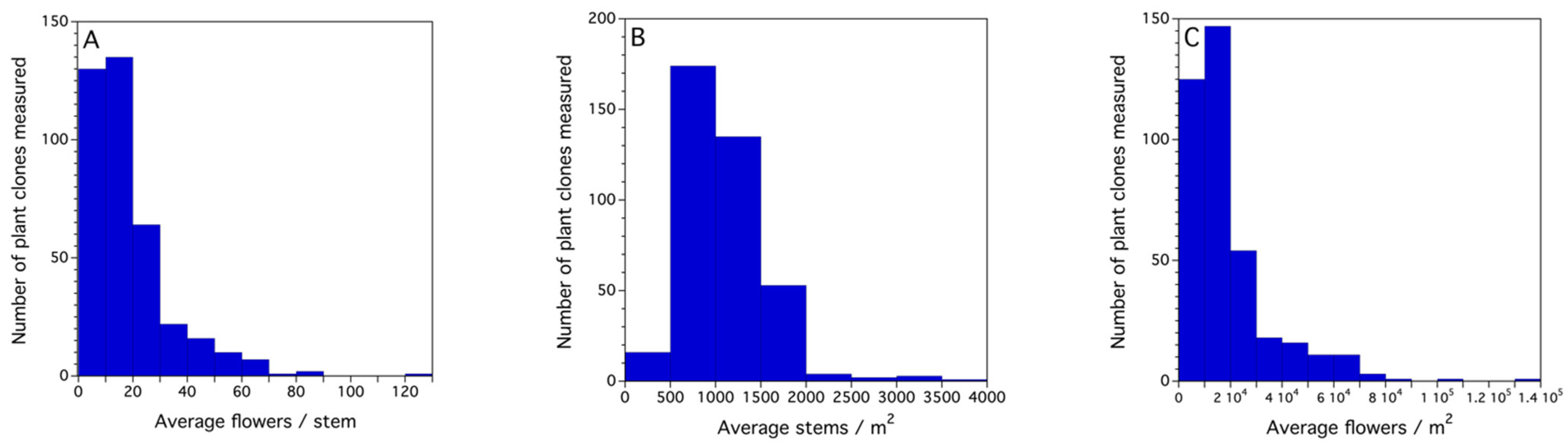
Flowers set per native bee/m² = as in case study 1, 22.9 flowers/stem × 738.4 stems/m² = 16,909.4 flowers /m². However, for honey bees, only a 1% fruit set/ bee/m² is expected [62], therefore 0.01 × 16,909.4 = 169.1 fruits, assuming a proportion of 0.364 (median) are dropped as in case study 1, thus 169.1 × (1 − 0.364) = 107.5 flowers/m². This number of flowers/m² is divided by 6.5. This factor determines the daily flowers available for visitation and thus, pollination per day, given the distributed bloom and the viability duration of 5 days once a flower is open. Therefore, in this case study, 107.5 flowers/m²/6.5 = 16.5 flowers/m² that will end up as marketable fruit at the end of the season. The observed frequency distributions of flowers/stem (Figure A1A), stems/m² (Figure A1B), and the derived estimate of flowers/m² (Figure A1C) are in Appendix A.

B =

Weight of one marketable berry is 0.0004 kg.

The equation becomes:

$$\mathrm{EPL}=\frac{\mathrm{USD} 0.075/{\mathrm{m}}^2}{\left(\mathrm{USD}1.50/\mathrm{kg} \mathrm{of} \mathrm{fruit}\times 16.5 \mathrm{fruits}/\mathrm{bee}/{\mathrm{m}}^2\times 0.0004 \mathrm{kg} \mathrm{of} \mathrm{fruit}\right)}$$

EPL = 7.6 honey bees/m²

(6)

The use of this equation with honey bees could be used to analyze the benefit of stocking honey bee colonies at 5 hives/ha. About 7.6 honey bees/m²/min would suggest that the stocking rate pays for itself in marketable fruit harvested, while less than this EPL suggests that the stocking rate is not paying for itself in returns from potential harvestable yield.

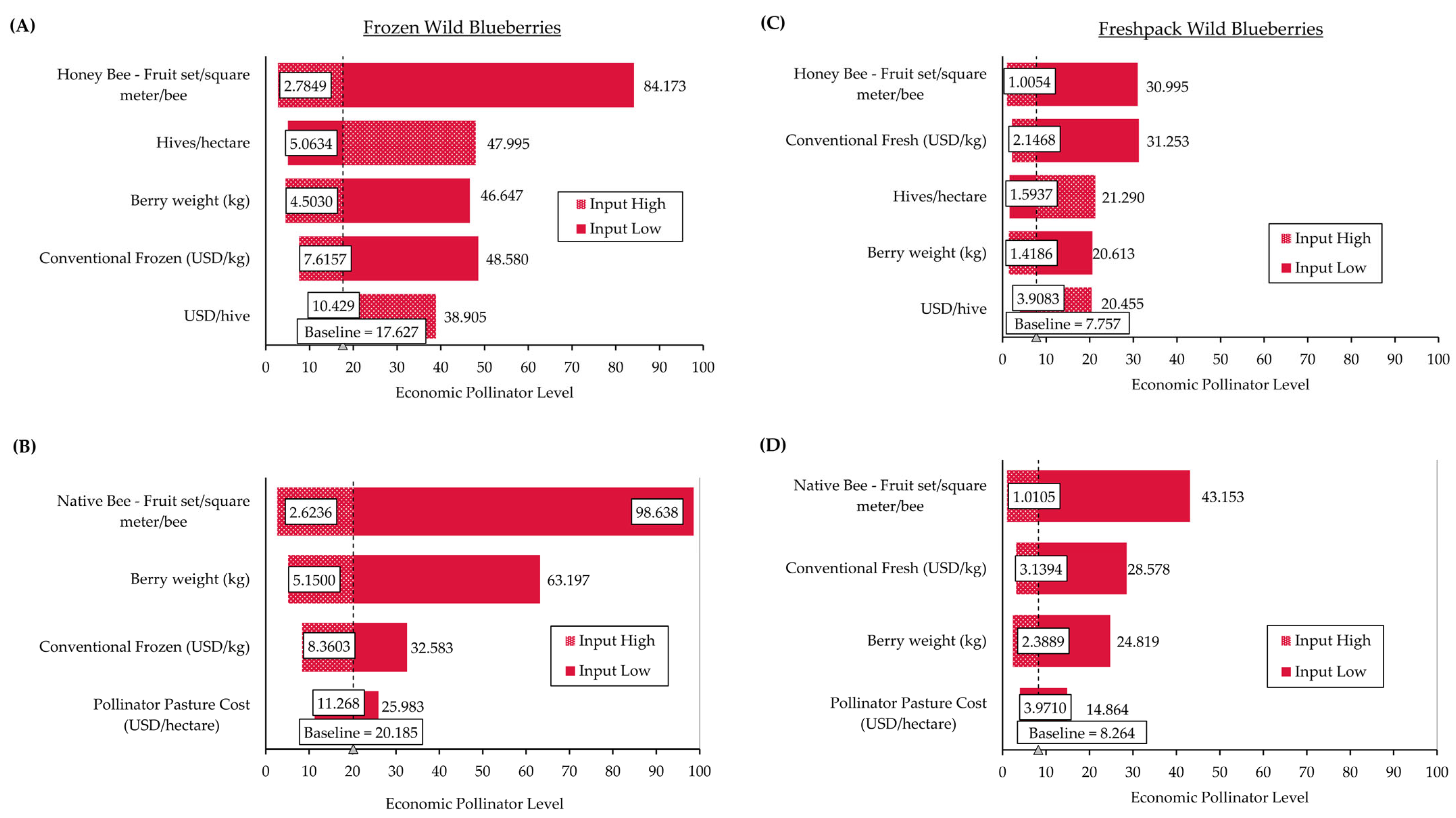
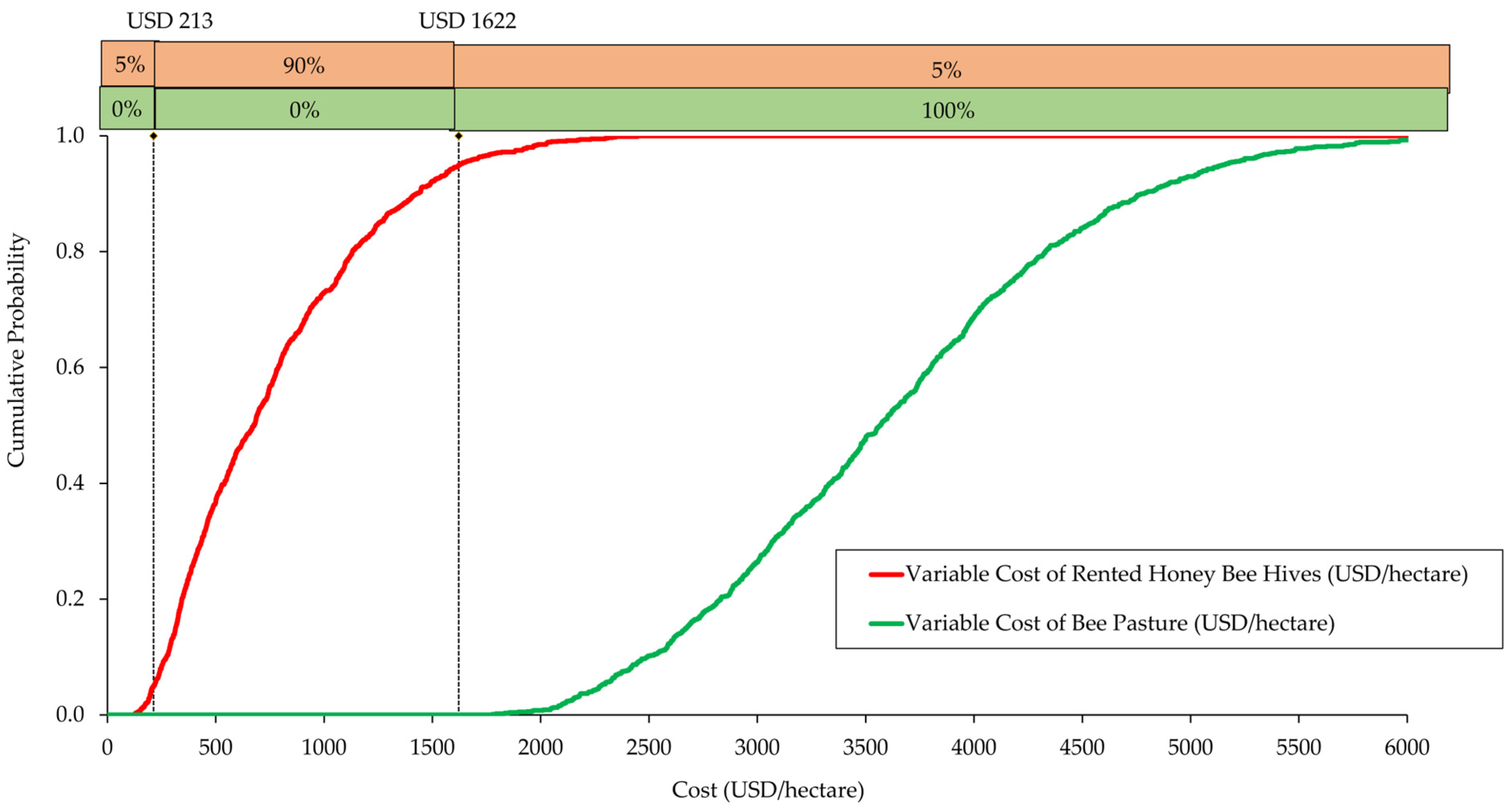
3.4. Monte Carlo Economic Simulations

The Economic Pollinator Level (EPL) is most sensitive to changes in fruit set by both honey bees and native bees regardless of frozen- or fresh-pack utilization for lowbush blueberries (Figure 6). There is greater sensitivity for frozen lowbush blueberries with EPL ranging from 2.785 to 84.173 for honey bees and ranging from 2.624 to 98.638 for native bees given stochastic changes in fruit set for both types of bees (Figure 6A,B). The sensitivity of EPL to changes in measured fruit set is less for both honey bees (1.005 to 30.995) and native bees (1.011 to 45.153) for fresh-pack lowbush blueberries (Figure 6C,D).

For honey bees pollinating lowbush blueberries, EPL is progressively less sensitive to stocking density (hives/hectare), berry weight (kg), and cost of rented hives (USD/hive), while lowbush blueberry prices impact EPL values more for fresh-pack versus frozen (Figure 6A,C). Similarly for native bee pollination of lowbush blueberries, EPL is less sensitive to berry weight (kg) and the cost of installing pollinator pasture (USD/hectare), while fresh-pack prices have a greater impact on EPL compared to frozen lowbush blueberry prices (Figure 6B,D).

4. Discussion

4.1. Interplay between Honey Bees and Native Bees in Lowbush Blueberry

Our research has shown that native bees (from genera Bombus, Andrenidae, Halictidae, Megachilidae, and Colletidae) and honey bees (Apis mellifera (L.)) are integral to the sweet lowbush blueberry (Vaccinium angustifolium Aiton) pollination system. Both wild native bees and commercially managed bees provide pollination services to lowbush blueberry, although different taxa of native wild bees have different spatial distributions within blueberry fields and different occurrences throughout bloom [77]. Different native bee species also vary in their explanatory power of fruit set in fields between years and studies [59,77,78,79]. Cutler et al. [77] studied lowbush blueberry pollination in Nova Scotia, Canada. They found more than 90% of the wild native bee community comprised individuals belonging to the genera Andrena and Lasioglossum. They also found that larger native bees were found in the interiors of fields, whereas smaller species were found along field edges.

Efficiency of pollination also varies by bee taxon. In our study, on a per bee basis, native bees are estimated to be about 10 times greater at setting fruit in lowbush blueberry (see mixed model coefficients in Table 2). This is greater than that reported by Asare et al. [26] who determined that wild native bees were 2.6 times more efficient lowbush blueberry pollinators on a per bee basis. Bushmann and Drummond [59] determined that wild native bees were about 5.5 times more efficient than honey bees as pollinators of lowbush blueberry in terms of the percentage of fruit set on a per bee basis. These different results for fruit set by bee taxon are supported by both field and laboratory experiments [71].

About 24% of growers in Maine rely extensively on native bees for their pollination needs, while the rest rely upon both honey bees and wild native bees [26]. Cutler et al. [77] found that, in Nova Scotia, most growers rely on honey bees for their pollination, similar to Maine. Bushmann and Drummond [59] determined that 36% of all foraging bees in lowbush blueberry fields are wild native bees. Those growers who rely only on wild native bees often have honey bees from neighboring growers foraging in their fields [26]. Those growers that rely upon wild native bees and who also supplement their foraging force with rented honey bee colonies benefit from their capital expenditure because most of their honey bees appear to forage within their fields. This is reflected by 42.5% of the variation in honey bee foragers counted in a field being explained by the hive density within that field. Asare et al. [26] showed a similar relationship with 55.5% of honey bee forager density being explained by hive density.

Both wild native bees and managed bees such as the honey bee are components of Maine lowbush blueberry pollination. The species co-occur and appear to complement each other in regard to providing a total fruit set that is a function of both types of bees together [26,59,61]. Previously, we found that honey bees do not appear to detrimentally affect native bee activity densities. Asare et al. [26], using a smaller collection of Maine bee community data for lowbush blueberry fields, found that the evidence of a negative interaction between honey bees and wild native bees is weak (p = 0.089), while Eaton and Nams [79] found evidence of a significant negative effect of honey bee populations on wild native bee abundance. However, it is difficult to know whether this negative interaction was because honey bees are often stocked in fields that have a historic low yield due to low wild native bee abundance.

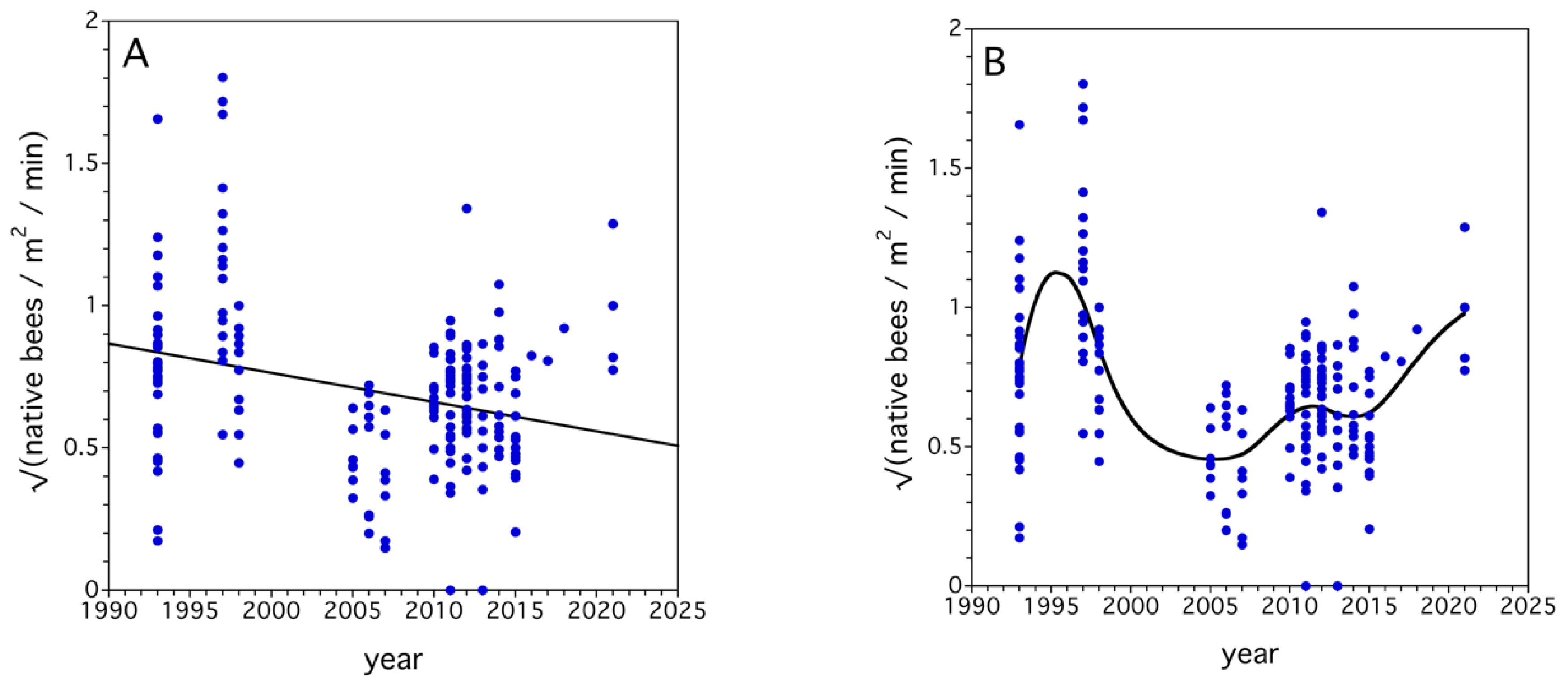
4.2. Long-Term Trends in Native Bee Communities

Our analysis provides evidence that when study project and year are accounted for as random effects, fruit set explains 52% of the variation in yield. Therefore, bees are potentially the most important input in lowbush blueberry production in Maine (see Yarborough et al. [80] for a quantification of the factors that affect lowbush blueberry yield). Bushmann and Drummond [59] found that a disruption of the supply of honey bees would result in a 30% reduction in yield. Estimates of the sole effect of wild native bees on the percentage of fruit set at the field level have been documented in several studies in both Maine and Canada, and range from 28% to 56% [26,59,81,82]. Based upon the importance of both honey bees and wild native bees in lowbush blueberry production, their conservation and enhancement should be a priority to growers.

However, bees appear to be in decline globally [83]. Population levels of honey bees are also in decline and without intensive management their survival rate is low [84]. Multiple causes of bee decline have been suggested, ranging from pesticide exposure, land-use changes, habitat destruction and reduction in natural bee forage, decline in genetic diversity, increase in disease and parasite virulence and incidence, and climate change [3,85]. Our study provides evidence that wild native bee abundance (Figure 5) may not be in decline, but that annual fluctuations can be extreme, making this natural resource and lowbush blueberry yields unpredictable from year to year. We do not have a long-term data set suggesting that bee species richness is declining in Maine lowbush blueberry. However, a five-year bumble bee survey throughout Maine suggests that some observed bumble bee species in the state no longer exist or are at densities difficult to detect (Maine Bumble Bee Atlas [86]) and that the decline of native pollinators is serious and should not be ignored, even if conclusive data do not exist for some areas, because they do exist for others [83,85,86].

4.3. Conservation of Honey Bees and Native Bees

Because of the global decline of wild native bee species richness, the annual and spatial variation in bee community abundances, and the decline in honey bee populations, conservation practices in agricultural cropping systems dependent upon bees are being formulated and implemented to sustain production [31,87,88,89]. The University of Maine Cooperative Extension Service has provided lowbush blueberry growers with guidance and technical bulletins on several approaches to conserving bee populations [90]. These approaches involve providing nest materials for Osmia spp. leafcutting and mason bees, reduction in pesticide risk to both wild native bees and honey bees by selecting the least toxic pesticides for application and reducing exposure [91,92], as well as planting pollinator pastures [31]. While these strategies have been shown to enhance bee abundance [31,93], there are still factors not in the control of growers that can result in the reduction in bee abundance or pollination in some years such as diseases and weather extremes [3,84,93].

4.4. Tools for Pollination Strategies

The University of Maine Cooperative Extension has also developed and provided training and tools for managing pollination on lowbush blueberry farms [88,90]. These involve recognition of wild native bee taxa, measuring bee foraging abundances in fields, measuring fruit set as a means of categorizing specific fields yield potential, and utilizing a spatial geographic mapping software tool which can identify bee habitats adjacent to specific blueberry fields and the size of associated wild native bee community abundance and predicted fruit set. These trainings and tools can not only be used to provide growers with the information they need to successfully conserve native bees, but they also allow them to determine levels of wild native bee abundances and then make decisions on whether honey bee rental is prudent and the stocking densities that can be considered. This knowledge of native bee and honey bee foraging abundances can also be used with the Economic Pollinator Level (EPL) tool developed in this study. The use of the EPL, as we have demonstrated, can allow lowbush blueberry growers to evaluate the economic rationale behind their pollination management plan.

4.5. Using Predictive Pollination Tools to Guide Pollinator Public Policy

Fruit set for lowbush blueberry was the primary driver of EPL (Figure 6). Fruit set in blueberry systems can be impacted by weather conditions during the May pollination window by affecting the number of pollination days, or more directly stated, the number of days that bees will be actively flying and visiting flowers [61,94]. While factors such as weather are beyond the control of lowbush blueberry producers, the decision to integrate pollinator pastures to provide floral resources for both managed and native bees is clearly within the control of producers. Despite the high total cost of planting pollinator pastures of ~USD 18,000/hectare (see Appendix A, Table A1) with the variable cost of planting ranging from USD 2000/ha to USD 6000/ha (Figure 7), the cost per hectare to plant these pastures has relatively low impact on variability of EPL values. The range of EPL values for pollinator pasture cost is lower compared to the range of EPL values for the cost of rented honey bee hives. This indicates greater efficiency of pollination investment for pollinator pastures compared to rented hives (Figure 6A versus Figure 6B and Figure 6C versus Figure 6D). This suggests that investing in native pollinator pastures can be a favorable investment in terms of EPL compared to renting migratory honey bee hives.

Although pollinator pastures may be an efficient EPL investment from a pollination perspective [31], there are challenges for lowbush blueberry producers to transition from renting honey bee hives to investing in pollinator pastures. Surveyed lowbush blueberry producers’ that planted pollinator pastures (15%) were smaller scale and less profitable than those that rent honey bee hives (77%) from migratory bee keepers [95]. Compared to other crops that have greater initial responsiveness to pollination from managed honey bees (e.g., cranberries), lowbush blueberries have more modest marginal returns to increasing rented hive stocking density, so lowbush blueberry producers are less willing to invest in on-farm wild bee habitats (USD 140/hectare) compared to USD 188/hectare for cranberry growers in Massachusetts, USA [27]. Potential adopters of pollinator enhancements such as those installing pollinator pasture in Maine’s lowbush blueberry industry, have been characterized as those who are more educated, use bumblebees, monitor bees, value the importance of native bees, rent fewer honey bee hives due to spillover pollination from neighbors, and those with farm landscapes that are more favorable to pollinators [96].

The total cost of pollinator pastures is most influenced by the ratio of pollinator pasture to lowbush blueberry crop area, as well as the stand life of the pollinator pasture, and is not influenced by variable input costs or the values of equipment used to install pastures (see Appendix A, Figure A2). Pollinator pastures become more costly if (1) more area has to be planted relative to lowbush blueberry crop area; or (2) pastures have to be re-seeded more often (e.g., pasture stand life of 2 to 3 years versus 10 years). Encouraging lowbush blueberry producers to invest in pollinator pastures may require subsidies of USD 2000 to USD 6000/hectare (Figure 7). Assuming that planted pollinator pastures comprise 10% of lowbush blueberry land area of 21,000 hectares [75] which equals 2100 hectares, the variable costs of installing pollinator pastures at this scale would range from USD 1.7 to 5 million. The variable cost range (USD 2000 to USD 6000/hectare) of pollinator pastures stochastically simulated in this study is consistent with recent increases in USDA-NRCS cost-share (60% to 75%) that would cover USD 1945 to USD 4411/ha for installing pollinator hedgerows on farms which increased participation in Maine, USA by 600% [27].

Our EPL results and stochastic simulations support arguments that pollination management should be based on direct measurement of pollinator activity [94]. While public policies around the world have focused on conservation of native pollinator habitat surrounding farms and/or pesticide regulation [97,98], such as in Brazil [42,99], Canada [100], and the United States of America [101], the focus in the European Union has shifted to Common Agricultural Policies [49,102] to encourage provision of ecosystem services such as pollination [103] by actively planting bee pastures [104]. Enhancing global pollination security using public policies directed at improving on-farm bee forage and habitat [54] is critical, not only in developed nations but also in developing nations [47]. Despite the recent introduction of public policies to improve pollination security over the past decade in the USA, these policies have been variable by state and region [105]. For example, 31 of 50 states in the USA have pollinator plans, with only Connecticut’s being legally binding [106]. Clearly there is room for improvement by better integrating data-driven pollination management (e.g., using EPL) to better guide regional pollinator plans and policies.

5. Conclusions

The lowbush blueberry production system in Maine and Canada is unique and requires a sustainable pollination force so that it remains economically viable or sustainable. Lowbush blueberry fields in Maine, USA, were surveyed for bees from 1993 to 2021 for honey bee and native bee activity densities, fruit set, and crop yield. Managed honey bee hive stocking density was also recorded if these pollinators were used. There were 209 lowbush blueberry fields in Maine sampled over these 29 years. As far as we know, this data set is the most extensive pollinator, fruit set, and yield survey in fields representing a single crop that exists globally. We statistically summarized these long-term data.

The proportion of fruit set in a field was predicted by both native bee and honey bee activity density. This relationship being highly statistically significant with a relatively high coefficient of determination shows how important foraging bee activity density is to fruit set, considering all of the other factors that affect fruit set in lowbush blueberry such as annual weather, regional climate differences, soil fertility, field-level blueberry genotype composition, pests and diseases, and crop management [26]. Honey bee activity density was well explained by hive stocking density. This is important because conduct of economic analyses or implementation of pollination tactics involving honey bee activity density goals must be performed using the unit of honey bee pollination, the hive [26,27,59,61]. The proportion of fruit set adequately predicted yield. Similar to the relationship between bee activity density and fruit set, there are many factors that affect yield in addition to fruit set [26,69,80,107,108]. These factors include the following: drought, pests and diseases, harvest method, intensity of pollination, soil fertility, fruit drop, method of harvest, and crop management.

We proposed and developed a novel indicator, the Economic Pollinator Level (EPL), to estimate bee densities that economically justify pollination investments such as rented hives and planting bee pastures given recent global declines in pollinators. The EPL equation determines adequate lowbush blueberry crop value (V), fruit set by pollinators (P), and the individual berry weight (B) that is sufficient to cover the cost (C) of either rented honey bee hives or establishing and maintaining pollinator pastures.

In order to determine the economic risk of pollination we used the EPL as a tool. Native bee and honey bee activity densities, honey bee hive stocking density, and native bees as a proportion of total bees in-field were all best fit to right-skewed distributions across sampled fields. The fruit set proportion was distributed as a symmetric Gaussian distribution across fields. Lowbush blueberry yield was best fit to a right-skewed Gamma probability distribution. These frequency distributions were the basis of the Monte Carlo simulations for assessing economic risk of pollination by way of the EPL. So, we stochastically varied V, P, and B from field surveyed and observational data, the EPL was found to be most sensitive to fruit set/m²/bee. Variation in berry weight, rented hive stocking density and price, lowbush blueberry prices, and annual cost of planting/maintaining pollinator pastures had less of an impact on EPL. The main contribution of this research demonstrates that the EPL can be used to better economize investments in managed honey bees, pollinator habitat, or any other pollinator tactic involving either or both wild native bees and managed bees. This can lead to agricultural systems, economic growth, employment opportunities, and invertebrate conservation investments that are more sustainable and durable over time. Future research could focus on using EPL for pollinator-dependent crops with adequate field data sets to better guide decisions on economically prudent investments in optimizing managed bee hive rentals, as well as planting bee pastures, selecting the least toxic pesticides, and constructing and maintaining wild bee nesting bare-ground habitats or twig-nesting bee habitats.

References

1. Pettis, J.S.; Delaplane, K.S. Coordinated responses to honey bee decline in the USA. Apidologie 2010, 41, 256–263. [Google Scholar] [CrossRef]
2. Tepedino, V.J.; Durham, S.; Cameron, S.A.; Goodell, K. Documenting bee decline or squandering scarce resources. Conserv. Biol. 2015, 29, 280–282. [Google Scholar] [CrossRef] [PubMed]
3. Goulson, D.; Nicholls, E.; Botías, C.; Rotheray, E.L. Bee declines driven by combined stress from parasites, pesticides, and lack of flowers. Science 2015, 347, 1255957. [Google Scholar] [CrossRef] [PubMed]
4. Soroye, P.; Newbold, T.; Kerr, J. Climate change contributes to widespread declines among bumble bees across continents. Science 2020, 367, 685–688. [Google Scholar] [CrossRef] [PubMed]
5. Mathiasson, M.E.; Rehan, S.M. Wild bee declines linked to plant-pollinator network changes and plant species introductions. Insect Conserv. Divers. 2020, 13, 595–605. [Google Scholar] [CrossRef]
6. Cariveau, D.P.; Winfree, R. Causes of variation in wild bee responses to anthropogenic drivers. Curr. Opin. Insect Sci. 2015, 10, 104–109. [Google Scholar] [CrossRef] [PubMed]
7. Scheper, J.; Reemer, M.; van Kats, R.; Ozinga, W.A.; van der Linden, G.T.; Schaminée, J.H.; Siepel, H.; Kleijn, D. Museum specimens reveal loss of pollen host plants as key factor driving wild bee decline in The Netherlands. Proc. Natl. Acad. Sci. USA 2014, 111, 17552–17557. [Google Scholar] [CrossRef] [PubMed]
8. Zayed, A. Bee genetics and conservation. Apidologie 2009, 40, 237–262. [Google Scholar] [CrossRef]
9. LeBuhn, G.; Luna, J.V. Pollinator decline: What do we know about the drivers of solitary bee declines? Curr. Opin. Insect Sci. 2021, 46, 106–111. [Google Scholar] [CrossRef]
10. Jacobson, M.M.; Tucker, E.M.; Mathiasson, M.E.; Rehan, S.M. Decline of bumble bees in northeastern North America, with special focus on Bombus terricola. Biol. Conserv. 2018, 217, 437–445. [Google Scholar] [CrossRef]
11. Bowers, M.A. Bumble Bee Colonization, Extinction, and Reproduction in Subalpine Meadows in Northeastern Utah: Ecological Archives E066-001. Ecology 1985, 66, 914–927. [Google Scholar] [CrossRef]
12. Buchmann, S.; Ascher, J.S. The plight of pollinating bees. Bee World 2005, 86, 71–74. [Google Scholar] [CrossRef]
13. Zattara, E.E.; Aizen, M.A. Worldwide occurrence records suggest a global decline in bee species richness. One Earth 2021, 4, 114–123. [Google Scholar] [CrossRef]
14. Colla, S.R.; Ascher, J.S.; Arduser, M.; Cane, J.; Deyrup, M.; Droege, S.; Gibbs, J.; Griswold, T.; Hall, H.G.; Henne, C.; et al. Documenting persistence of most eastern North American bee species (Hymenoptera: Apoidea: Anthophila) to 1990–2009. J. Kans. Entomol. Soc. 2012, 85, 14–22. [Google Scholar] [CrossRef]
15. Hamblin, A.L.; Youngsteadt, E.; Frank, S.D. Wild bee abundance declines with urban warming, regardless of floral density. Urban Ecosyst. 2018, 21, 419–428. [Google Scholar] [CrossRef]
16. Lebuhn, G.; Droege, S.; Connor, E.F.; Gemmill-Herren, B.; Potts, S.G.; Minckley, R.L.; Griswold, T.; Jean, R.; Kula, E.; Roubik, D.W.; et al. Detecting insect pollinator declines on regional and global scales. Conserv. Biol. 2013, 27, 113–120. [Google Scholar] [CrossRef] [PubMed]
17. Roubik, D.W. Ups and downs in pollinator populations: When is there a decline? Conserv. Ecol. 2001, 5. Available online: https://www.jstor.org/stable/26271795 (accessed on 2 November 2023). [CrossRef]
18. Decourtye, A.; Alaux, C.; Le Conte, Y.; Henry, M. Toward the protection of bees and pollination under global change: Present and future perspectives in a challenging applied science. Curr. Opin. Insect Sci. 2019, 35, 123–131. [Google Scholar] [CrossRef] [PubMed]
19. Otto, C.R.; Zheng, H.; Gallant, A.L.; Iovanna, R.; Carlson, B.L.; Smart, M.D.; Hyberg, S. Past role and future outlook of the Conservation Reserve Program for supporting honey bees in the Great Plains. Proc. Natl. Acad. Sci. USA 2018, 115, 629–7634. [Google Scholar] [CrossRef]
20. Winfree, R.; Gross, B.J.; Kremen, C. Valuing pollination services to agriculture. Ecol. Econ. 2011, 71, 80–88. [Google Scholar] [CrossRef]
21. Carreck, N.; Williams, I. The economic value of bees in the UK. Bee World 1998, 79, 115–123. [Google Scholar] [CrossRef]
22. Southwick, E.E.; Southwick, L., Jr. Estimating the economic value of honey bees (Hymenoptera: Apidae) as agricultural pollinators in the United States. J. Econ. Entomol. 1992, 85, 621–633. [Google Scholar] [CrossRef]
23. Calderone, N.W. Insect pollinated crops, insect pollinators and US agriculture: Trend analysis of aggregate data for the period 1992–2009. PLoS ONE 2012, 7, e37235. [Google Scholar] [CrossRef] [PubMed]
24. Losey, J.E.; Vaughan, M. The economic value of ecological services provided by insects. Bioscience 2006, 56, 311–323. [Google Scholar] [CrossRef]
25. Garibaldi, L.A.; Aizen, M.A.; Klein, A.M.; Cunningham, S.A.; Harder, L.D. Global growth and stability of agricultural yield decrease with pollinator dependence. Proc. Natl. Acad. Sci. USA 2011, 108, 5909–5914. [Google Scholar] [CrossRef] [PubMed]
26. Asare, E.; Hoshide, A.K.; Drummond, F.A.; Chen, X.; Criner, G.K. Economic risk of bee pollination in Maine wild blueberry, Vaccinium angustifolium Aiton. J. Econ. Entomol. 2017, 110, 1980–1992. [Google Scholar] [CrossRef] [PubMed]
27. Hoshide, A.K.; Drummond, F.A.; Stevens, T.H.; Venturini, E.M.; Hanes, S.P.; Sylvia, M.M.; Loftin, C.S.; Yarborough, D.E.; Averill, A.L. What is the value of wild bee pollination for wild blueberries and cranberries and who values it? Environments 2018, 5, 98. [Google Scholar] [CrossRef]
28. Khalifa, S.A.; Elshafiey, E.H.; Shetaia, A.A.; El-Wahed, A.A.A.; Algethami, A.F.; Musharraf, S.G.; AlAjmi, M.F.; Zhao, C.; Masry, S.H.; Abdel-Daim, M.M.; et al. Overview of bee pollination and its economic value for crop production. Insects 2021, 12, 688. [Google Scholar] [CrossRef]
29. Gallai, N.; Salles, J.M.; Settele, J.; Vaissière, B.E. Economic valuation of the vulnerability of world agriculture confronted with pollinator decline. Ecol. Econ. 2009, 68, 810–821. [Google Scholar] [CrossRef]
30. Lippert, C.; Feuerbacher, A.; Narjes, M. Revisiting the economic valuation of agricultural losses due to large-scale changes in pollinator populations. Ecol. Econ. 2021, 180, 106860. [Google Scholar] [CrossRef]
31. Venturini, E.M.; Drummond, F.A.; Hoshide, A.K.; Dibble, A.C.; Stack, L.B. Pollination reservoirs in Maine lowbush blueberry (Ericales: Ericaceae). J. Econ. Entomol. 2017, 110, 333–346. [Google Scholar] [CrossRef] [PubMed]
32. Albrecht, M.; Kleijn, D.; Tschumi, M.; Blaauw, B.R.; Bommarco, R.; Campbell, A.; Dainese, M.; Drummond, F.A.; Entling, M.; Ganser, D.; et al. A quantitative synthesis reveals flower plantings underpinning ecological intensification through enhanced pest control services and identifies drivers of increased crop pollination services. Ecol. Lett. 2020, 23, 1488–1498. [Google Scholar] [CrossRef] [PubMed]
33. Egan, P.A.; Dicks, L.V.; Hokkanen, H.M.; Stenberg, J.A. Delivering integrated pest and pollinator management (IPPM). Trends Plant Sci. 2020, 25, 577–589. [Google Scholar] [CrossRef] [PubMed]
34. McDougall, R.; DiPaola, A.; Blaauw, B.; Nielsen, A.L. Managing orchard groundcover to reduce pollinator foraging post-bloom. Pest Manag. Sci. 2021, 77, 3554–3560. [Google Scholar] [CrossRef] [PubMed]
35. Habel, J.C.; Samways, M.J.; Schmitt, T. Mitigating the precipitous decline of terrestrial European insects: Requirements for a new strategy. Biodivers. Conserv. 2019, 28, 1343–1360. [Google Scholar] [CrossRef]
36. Papanikolaou, A.D.; Kühn, I.; Frenzel, M.; Schweiger, O. Semi-natural habitats mitigate the effects of temperature rise on wild bees. J. Appl. Ecol. 2017, 54, 527–536. [Google Scholar] [CrossRef]
37. Klaus, F.; Tscharntke, T.; Bischoff, G.; Grass, I. Floral resource diversification promotes solitary bee reproduction and may offset insecticide effects–evidence from a semi-field experiment. Ecol. Lett. 2021, 24, 668–675. [Google Scholar] [CrossRef] [PubMed]
38. Kline, O.; Joshi, N.K. Mitigating the effects of habitat loss on solitary bees in agricultural ecosystems. Agriculture 2020, 10, 115. [Google Scholar] [CrossRef]
39. Durant, J.L.; Otto, C.R. Feeling the sting? Addressing land-use changes can mitigate bee declines. Land Use Policy 2019, 87, 104005. [Google Scholar] [CrossRef]
40. Senapathi, D.; Biesmeijer, J.C.; Breeze, T.D.; Kleijn, D.; Potts, S.G.; Carvalheiro, L.G. Pollinator conservation—The difference between managing for pollination services and preserving pollinator diversity. Curr. Opin. Insect Sci. 2015, 12, 93–101. [Google Scholar] [CrossRef]
41. Hall, D.M.; Steiner, R. Policy content analysis: Qualitative method for analyzing sub-national insect pollinator legislation. MethodsX 2020, 7, 100787. [Google Scholar] [CrossRef]
42. Hipólito, J.; Coutinho, J.; Mahlmann, T.; Santana, T.B.R.; Magnusson, W.E. Legislation and pollination: Recommendations for policymakers and scientists. Perspect. Ecol. Conserv. 2021, 19, 1–9. [Google Scholar] [CrossRef]
43. Faichnie, R.; Breeze, T.D.; Senapathi, D.; Garratt, M.P.; Potts, S.G. Scales matter: Maximising the effectiveness of interventions for pollinators and pollination. Adv. Ecol. Res. 2021, 64, 105–147. [Google Scholar] [CrossRef]
44. Maderson, S.; Wynne-Jones, S. Beekeepers’ knowledges and participation in pollinator conservation policy. J. Rural Stud. 2016, 45, 88–98. [Google Scholar] [CrossRef]
45. Baldock, K.C.R. Opportunities and threats for pollinator conservation in global towns and cities. Curr. Opin. Insect Sci. 2020, 38, 63–71. [Google Scholar] [CrossRef]
46. Breeze, T.D.; Gallai, N.; Garibaldi, L.A.; Li, X.S. Economic measures of pollination services: Shortcomings and future directions. Trends Ecol. Evol. 2016, 31, 927–939. [Google Scholar] [CrossRef]
47. Porto, R.G.; de Almeida, R.F.; Cruz-Neto, O.; Tabarelli, M.; Viana, B.F.; Peres, C.A.; Lopes, A.V. Pollination ecosystem services: A comprehensive review of economic values, research funding and policy actions. Food Secur. 2020, 12, 1425–1442. [Google Scholar] [CrossRef]
48. United Nations (U.N.). The 17 Goals: Sustainable Development Goals. Department of Economic and Social Affairs, Sustainable Development. Available online: https://sdgs.un.org/goals (accessed on 16 January 2024).
49. Cole, L.J.; Kleijn, D.; Dicks, L.V.; Stout, J.C.; Potts, S.G.; Albrecht, M.; Balzan, M.V.; Bartomeus, I.; Bebeli, P.J.; Bevk, D.; et al. A critical analysis of the potential for EU common agricultural policy measures to support wild pollinators on farmland. J. Appl. Ecol. 2020, 57, 681–694. [Google Scholar] [CrossRef] [PubMed]
50. Potts, S.G.; Biesmeijer, J.C.; Bommarco, R.; Felicioli, A.; Fischer, M.; Jokinen, P.; Kleijn, D.; Klein, A.M.; Kunin, W.E.; Neumann, P.; et al. Developing European conservation and mitigation tools for pollination services: Approaches of the STEP (Status and Trends of European Pollinators) project. J. Apic. Res. 2011, 50, 152–164. [Google Scholar] [CrossRef]
51. Dicks, L.V.; Baude, M.; Roberts, S.P.; Phillips, J.; Green, M.; Carvell, C. How much flower-rich habitat is enough for wild pollinators? Answering a key policy question with incomplete knowledge. Ecol. Entomol. 2015, 40, 22–35. [Google Scholar] [CrossRef]
52. Potts, S.G.; Ngo, H.T.; Biesmeijer, J.C.; Breeze, T.D.; Dicks, L.V.; Garibaldi, L.A.; Hill, R.; Settele, J.; Vanbergen, A. The assessment report of the Intergovernmental Science-Policy Platform on Biodiversity and Ecosystem Services on pollinators, pollination and food production. In IPBES (2016): Summary for Policymakers of the Assessment Report of the Intergovernmental Science-Policy Platform on Biodiversity and Ecosystem Services on Pollinators, Pollination and Food Production; Secretariat of the Intergovernmental Science-Policy Platform on Biodiversity and Ecosystem Services: Bonn, Germany, 2016; 36p, ISBN 978-92-807-3568-0. [Google Scholar]
53. Williams, I.H. Insect pollination and crop production: A European perspective. In Pollinating Bees–The Conservation Link between Agriculture and Nature; Kevan, P., Imperatriz, F.V.L., Eds.; Ministry of the Environment: Brasilia, Brazil, 2002; pp. 59–65. Available online: https://grist.org/wp-content/uploads/2012/01/livro_02_willians.pdf (accessed on 8 January 2024).
54. Dicks, L.V.; Viana, B.; Bommarco, R.; Brosi, B.; Arizmendi, M.; Cunningham, S.A.; Galetto, L.; Hill, R.; Lopes, A.V.; Pires, C.; et al. Ten policies for pollinators. Science 2016, 354, 975–976. [Google Scholar] [CrossRef] [PubMed]
55. Rose, T.; Kremen, C.; Thrupp, A. Policy Analysis Paper: Policy Mainstreaming of Biodiversity and Ecosystem Services with a Focus on Pollination; FAO: Rome, Italy, 2014; Available online: https://escholarship.org/uc/item/4p8419st (accessed on 2 November 2023).
56. Bloom, E.H.; Graham, K.K.; Haan, N.L.; Heck, A.R.; Gut, L.J.; Landis, D.A.; Milbrath, M.O.; Quinlan, G.M.; Wilson, J.K.; Zhang, Y.; et al. Responding to the US national pollinator plan: A case study in Michigan. Front. Ecol. Environ. 2022, 20, 84–92. [Google Scholar] [CrossRef]
57. Garibaldi, L.A.; Pérez-Méndez, N.; Garratt, M.P.; Gemmill-Herren, B.; Miguez, F.E.; Dicks, L.V. Policies for ecological intensification of crop production. Trends Ecol. Evol. 2019, 34, 282–286. [Google Scholar] [CrossRef] [PubMed]
58. Yarborough, D.E. Establishment and management of the cultivated lowbush blueberry (Vaccinium angustifolium). Internat. J. Fruit Sci. 2012, 12, 14–22. [Google Scholar] [CrossRef]
59. Bushmann, S.A.; Drummond, F.A. Analysis of Pollination Services Provided by Wild and Managed Bees (Apoidea) in Wild Blueberry (Vaccinium angustifolium Aiton) Production in Maine, USA, with a Literature Review. Agronomy 2020, 10, 1413. [Google Scholar] [CrossRef]
60. Drummond, F.A. Wild Blueberry Annual Research Reports; University of Maine: Orono, ME, USA, 2024. [Google Scholar]
61. Qu, H.; Drummond, F.A. Simulation-based modeling of wild blueberry pollination. Comput. Electron. Agric. 2018, 144, 94–101. [Google Scholar] [CrossRef]
62. SAS Institute. JMP(R), Version 16; SAS Institute Inc.: Cary, NC, USA, 2022.
63. Palisade. Guide to Using @Risk: Risk Analysis and Simulation Add-In for Microsoft Excel; Version 7.5; Palisade Corporation: New Field, NY, USA, 2016. [Google Scholar]
64. Hardaker, J.B.; Huirne, R.B.M.; Anderson, J.R.; Lien, G. Coping with Risk in Agriculture, 3rd ed.; CAB International Publishing: Oxfordshire, UK, 2015; pp. 1–289. [Google Scholar]
65. Hummel, R.M.; Claassen, E.A.; Wolfinger, R.D. JMP for Mixed Models; SAS Institute Incorporated; SAS Campus Drive: Cary, NC, USA, 2021; pp. 1–243. Available online: https://www.jmp.com/en_us/whitepapers/book-chapters/jmp-for-mixed-models.html (accessed on 5 April 2024).
66. Boker, B.M.; Brooks, M.E.; Clark, C.J.; Geange, S.W.; Poulsen, J.R.; Stevens, M.H.H.; White, J.-S.S. General linear mixed models: A practical guide for ecology and evolution. Trends Ecol. Evol. 2009, 24, 127–135. [Google Scholar] [CrossRef] [PubMed]
67. Box, G.E.; Jenkins, G.M.; Reinsel, G.C.; Ljung, G.M. Time Series Analysis: Forecasting and Control, 5th ed.; John Wiley & Sons: Hoboken, NJ, USA, 2015; 712p, ISBN 978-1-118-67502-1. [Google Scholar]
68. Stern, V.M.; Smith, R.F.; Van Den Bosch, R.; Hagen, K.S. The integrated control concept. Hilgardia 1959, 29, 81–101. [Google Scholar] [CrossRef]
69. Pedigo, K.P.; Hutchins, S.H.; Higley, L.G. Economic injury levels in theory and practice. Annu. Rev. Entomol. 1986, 31, 341–368. [Google Scholar] [CrossRef]
70. Javorek, S.K.; MacKenzie, K.E.; Kloet, S.P.V. Comparative Pollination Effectiveness among Bees (Hymenoptera: Apoidea) on Lowbush Blueberry (Ericaceae: Vaccinium angustifolium). Ann. Entomol. Soc. Am. 2002, 95, 345–351. [Google Scholar] [CrossRef]
71. Drummond, F.A. Reproductive biology of wild blueberry (Vaccinium angustifolium Aiton). Agriculture 2019, 9, 69. [Google Scholar] [CrossRef]
72. U.S. Bureau of Labor Statistics. Data Tools, Data Retrieval Tools, Series Report. Available online: https://data.bls.gov/cgi-bin/srgate (accessed on 10 November 2023).
73. International Monetary Fund. Producer Price Index Manual: Theory and Practice. Manuals and Guides. 2004. Available online: https://www.imf.org/en/Publications/Manuals-Guides/Issues/2016/12/30/Producer-Price-Index-Manual-Theory-and-Practice-16966 (accessed on 7 December 2023).
74. U.S. Department of Agriculture, National Agricultural Statistics Service. Quick Stats. Available online: https://quickstats.nass.usda.gov/results/A2524626-1096-3EF6-A6D7-CF842A803783 (accessed on 10 November 2023).
75. Langemeier, M. Trends in General Inflation and Farm Input Prices. Center for Commercial Agriculture, Purdue University. 2022. Available online: https://ag.purdue.edu/commercialag/home/wp-content/uploads/2022/04/20220429_Langemeier-TrendsInGeneralInflationAndFarmInputPrices.pdf (accessed on 7 December 2023).
76. David, A. Freedman. Statistical Models: Theory and Practice; Cambridge University Press: Cambridge, UK, 2009; pp. 1–458. ISBN 978-1-139-47731-4. [Google Scholar]
77. Cutler, G.C.; Nams, V.O.; Craig, P.; Sproule, J.M.; Sheffield, C.S. Wild bee pollinator communities of lowbush blueberry fields: Spatial and temporal trends. Basic Appl. Ecol. 2015, 16, 73–85. [Google Scholar] [CrossRef]
78. Eaton, L.J.; Murray, J.E. Relationships of pollinator numbers in blueberry fields to fruit development and yields. Acta Hortic. 1997, 446, 181–188. [Google Scholar] [CrossRef]
79. Eaton, L.J.; Nams, V.O. Honeybee stocking numbers and wild blueberry production in Nova Scotia. Can. J. Plant Sci. 2012, 92, 1305–1310. [Google Scholar] [CrossRef]
80. Yarborough, D.; Drummond, F.; Annis, S.; D’Appollonio, J. Maine Wild blueberry systems analysis. Acta Hort. 2017, 1180, 151–160. [Google Scholar] [CrossRef]
81. Boulanger, L.W. Blueberry pollination and solitary bees. Maine Farm Res. 1964, 12, 5–11. [Google Scholar]
82. Desjardins, E.; de Oliveira, D. Commercial bumble bee Bombus impatiens (Hymenoptera: Apidae) as a pollinator in lowbush blueberry (Ericale: Ericaceae) fields. J. Econ. Entomol. 2006, 99, 443–449. [Google Scholar] [CrossRef] [PubMed]
83. Potts, S.G.; Imperatriz-Fonseca, V.; Ngo, H.T.; Aizen, M.A.; Biesmeijer, J.C.; Breeze, T.D.; Dicks, L.V.; Garibaldi, L.; Hill, R.; Settele, J.; et al. Safeguarding Pollinators and Their Values to Human Well-being. Nature 2016, 540, 220–229. [Google Scholar] [CrossRef]
84. Evans, J.D.; Chen, Y. Colony collapse disorder and honey bee health. In Honey Bee Medicine for the Veterinary Practitioner, 1st ed.; Kane, T.R., Faux, C.M., Eds.; John Wiley & Sons, Inc.: New York, NY, USA, 2021; Chapter 19; pp. 229–234. ISBN 9781119583417. [Google Scholar] [CrossRef]
85. Kerr, J.T.; Pindar, A.; Galpern, P.; Packer, L.; Potts, S.G.; Roberts, S.M.; Rasmont, P.; Schweiger, O.; Colla, S.R.; Richardson, L.L. Climate Change Impacts on Bumblebees Converge Across Continents. Science 2015, 349, 177–180. [Google Scholar] [CrossRef]
86. Maine Bee Atlas. Available online: https://mainebumblebeeatlas.umf.maine.edu (accessed on 16 January 2024).
87. Scheper, J.A. Promoting wild bees in European agricultural landscapes. Alterra Sci. Contrib. 2015, 47, 1–176. Available online: https://www.wur.nl/upload_mm/c/b/a/a738b550-9f10-48ba-aa17-ef1755804127_Scheper_2015_PhD%20thesis_Promoting%20wild%20bees%20in%20European%20agricultural%20landscapes.pdf (accessed on 5 January 2024).
88. Isaacs, R.; Williams, N.; Ellis, J.; Pitts-Singer, T.L.; Bommarco, R.; Vaughan, M. Integrated crop pollination: Combining strategies to ensure stable and sustainable yields of pollination-dependent crops. Basic Appl. Ecol. 2017, 22, 44–60. [Google Scholar] [CrossRef]
89. Cortés-Rivas, B.; Monzón, V.H.; Rego, J.O.; Mesquita-Neto, J.N. Pollination by native bees achieves high fruit quantity and quality of highbush blueberry: A sustainable alternative to managed pollinators. Front. Sustain. Food Syst. 2023, 7, 1142623. [Google Scholar] [CrossRef]
90. Cooperative Extension Wild Blueberries. Available online: https://extension.umaine.edu/blueberries/ (accessed on 15 January 2024).
91. Fanning, P.; Collins, J. 2023 Insect Pest Management Guide: Insects. University of Maine Cooperative Extension, Maine Wild Blueberries. Available online: https://extension.umaine.edu/blueberries/wp-content/uploads/sites/41/2022/02/2022-insecticide-chart.pdf (accessed on 13 January 2024).
92. Markuson, J. Integrated Pest Pollinator Management. In Proceedings of the NRCS Bee Conservation Presentation, 2020 Wild Blueberry Conference, Bangor, ME, USA, 22 February 2020; Available online: https://extension.umaine.edu/blueberries/integrated-pest-and-pollinator-management-ippm/ (accessed on 13 December 2023).
93. Blaauw, B.R.; Isaacs, R. Flower plantings increase wild bee abundance and the pollination services provided to a pollination-dependent crop. J. Appl. Ecol. 2014, 51, 890–898. [Google Scholar] [CrossRef]
94. Tuell, J.K.; Isaacs, R. Weather during bloom affects pollination and yield of highbush blueberry. J. Econ. Entomol. 2010, 103, 557–562. [Google Scholar] [CrossRef] [PubMed]
95. Hanes, S.P.; Collum, K.K.; Hoshide, A.K.; Asare, E. Grower perceptions of native pollinators and pollination strategies in the lowbush blueberry industry. Renew. Agric. Food Syst. 2015, 30, 124–131. [Google Scholar] [CrossRef]
96. Hanes, S.P.; Collum, K.K.; Drummond, F.A.; Hoshide, A.K. Assessing Wild Pollinators in Conventional Agriculture: A Case Study from Maine’s Blueberry Industry. Hum. Ecol. Rev. 2018, 24, 97–113. [Google Scholar] [CrossRef]
97. Gemmill-Herren, B.; Garibaldi, L.A.; Kremen, C.; Ngo, H.T. Building effective policies to conserve pollinators: Translating knowledge into policy. Curr. Opin. Insect Sci. 2021, 46, 64–71. [Google Scholar] [CrossRef] [PubMed]
98. Nicholls, A.A.; Epstein, G.B.; Colla, S.R. Understanding public and stakeholder attitudes in pollinator conservation policy development. Environ. Sci. Policy 2020, 111, 27–34. [Google Scholar] [CrossRef]
99. Galetto, L.; Aizen, M.A.; Arizmendi, M.D.C.; Freitas, B.M.; Garibaldi, L.A.; Giannini, T.C.; Lopes, A.V.; Santo, M.M.D.E.; Maués, M.M.; Nates-Parra, G.; et al. Risks and opportunities associated with pollinators’ conservation and management of pollination services in Latin America. Ecol. Austral 2022, 32, 55–76. [Google Scholar] [CrossRef]
100. Nalepa, R.; Colla, S.R. Toward a wild pollinator strategy for Canada: Expert-recommended solutions and policy levers. FACETS 2023, 8, 1–18. [Google Scholar] [CrossRef]
101. Vanegas, M. The Silent Beehive. Ecol. Law Q. 2017, 44, 311–342. [Google Scholar] [CrossRef]
102. Giovanetti, M.; Bortolotti, L. Pollinators and policy: The intersecting path of various actors across an evolving CAP. Renew. Agric. Food Syst. 2023, 38, e27. [Google Scholar] [CrossRef]
103. Ratamäki, O.; Jokinen, P.; Sørensen, P.B.; Breeze, T.D.; Potts, S. A multilevel analysis on pollination-related policies. Ecosyst. Serv. 2015, 14, 133–143. [Google Scholar] [CrossRef]
104. Steele, D.J.; Baldock, K.C.R.; Breeze, T.D.; Brown, M.J.F.; Carvell, C.; Dicks, L.V.; Garratt, M.P.; Norman, H.; Potts, S.G.; Senapathi, D.; et al. Management and Drivers of Change of Pollinating Insects and Pollination Services. National Pollinator Strategy: For Bees and Other Pollinators in England, Evidence Statements and Summary of Evidence; Project Report; Department for Environment, Food and Rural Affairs: London, UK, 2019; pp. 1–91. Available online: https://nrl.northumbria.ac.uk/id/eprint/42117/ (accessed on 7 January 2024).
105. Hall, D.M.; Steiner, R. Insect pollinator conservation policy innovations at subnational levels: Lessons for lawmakers. Environ. Sci. Policy 2019, 93, 118–128. [Google Scholar] [CrossRef]
106. Whitney, K.S.; Stringer, B.B. Evaluation of US state pollinator plans using 3 evidence-based policymaking frameworks. bioRxiv 2021. [Google Scholar] [CrossRef]
107. Drummond, F.A. Factors that affect yield in wild blueberry, Vaccinium angustifolium Aiton. Agric. Res. Technol. 2019, 22, 556212. [Google Scholar] [CrossRef]
108. Drummond, F.A. Wild blueberry fruit drop: A consequence of seed set? Special Issue: Pollinator Diversity and Pollination in Agricultural Systems. Agronomy 2020, 10, 939. [Google Scholar] [CrossRef]
109. Neal, C. University of New Hampshire Cooperative Extension. Planting for Pollinators: Establishing a Wildflower Meadow from Seed. Fact Sheet. 2019. Available online: https://extension.unh.edu/sites/default/files/migrated_unmanaged_files/Resource007652_Rep11219.pdf (accessed on 10 November 2023).
110. OPN Seed. Eastern Great Lakes Native Pollinator Seed Mix. Available online: https://www.opnseed.com/products/eastern-great-lakes-native-pollinator-mix?variant=40552977694918 (accessed on 10 November 2023).
111. Wong, D. Peace Region Forage Seed Association. Historical Grass and Legume Seed Prices: 1970 to 2016. White Paper, 2017; pp. 1–4. Available online: http://www.peaceforageseed.ca/pdf/markets_2013_onwards/2017/Historical_prices_to_2016.pdf (accessed on 10 November 2023).
112. U.S. Geological Survey, National Minerals Information Center. Vermiculite–Historical Statistics (Data Series 140). 2020. Available online: https://www.usgs.gov/media/files/vermiculite-historical-statistics-data-series-140 (accessed on 10 November 2023).
113. U.S. Department of Agriculture, Economic Research Service. Real Wages for U.S. Nonsupervisory Farm and Nonfarm Workers, 1990–2022. Available online: https://www.ers.usda.gov/webdocs/charts/63462/wagerates2022linesbar_d.html?v=5868.1 (accessed on 10 November 2023).
114. U.S. Department of Agriculture, Agricultural Marketing Service. Historical Diesel Fuel Prices, Annual Average U.S. On-Highway Diesel Fuel Prices ($/gallon). Available online: https://agtransport.usda.gov/Fuel/Historical-Diesel-Fuel-Prices/u2kh-s8ke (accessed on 10 November 2023).
115. Hoshide, A.K.; Dalton, T.J.; Smith, S.N. Profitability of coupled potato and dairy farms in Maine. Renew. Agric. Food Sys. 2006, 21, 261–272. [Google Scholar] [CrossRef]
116. Lazarus, W.F. Machinery Cost Estimates (2004, 2008, 2012, 2013, 2021, and 2023). University of Minnesota Extension. Available online: https://wlazarus.cfans.umn.edu/william-f-lazarus-farm-machinery-management (accessed on 10 November 2023).
117. U.S. Department of Agriculture, Economic Research Service. Average U.S. Farm Real Estate Value, Nominal and Real (Inflation Adjusted), 1970–2020. Available online: https://www.ers.usda.gov/webdocs/charts/55910/farmrealestatevalue2020_d.html?v=9097.6 (accessed on 10 November 2023).
118. Maine Revenue Services. Estimated Full Value Tax Rates (2012–2021). Available online: https://www.maine.gov/revenue/sites/maine.gov.revenue/files/inline-files/fullvaluerates.pdf (accessed on 10 November 2023).
Figure 1. Observed frequency distributions (blue bars) and best fitting probability density functions (green bars) to bee community measures in 209 lowbush blueberry fields, activity density of (A) native bees, activity density of (B) honey bees, (C) hives/ha, and (D) proportion of native bee activity density to total bee activity density in Maine, USA.
Sustainability 16 03242 g001aSustainability 16 03242 g001b
Figure 2. Observed frequency distributions (blue bars) and best fitting probability density functions (green bars) to pollination measures in 209 lowbush blueberry fields for (A) fruit set and (B) yield in Maine, USA.
Sustainability 16 03242 g002
Figure 3. The (A) relationship between honey bee hive stocking density and honey bee activity density (honey bees/m2/min), and the (B) relationship between percentage of fruit set and yield (kg/ha) in Maine, USA.
Sustainability 16 03242 g003
Figure 4. The (A) relationship between the square root transformed cost of honey bee hives/hectare that farmers will invest in increasing hive stocking density and the resulting monetary value (USD) of the harvested crop (berries) per hectare; and (B) the relationship between the stocking density of honey bee hives/hectare (power transformed, xa) and the ratio of blueberry crop value (USD) to the dollar value (USD) of investment in honey bee hive rental by growers in Maine, USA.
Sustainability 16 03242 g004
Figure 5. Native bee activity density time series in Maine, USA, where densities are square root transformed using (A) linear regression and (B) non-linear spline smoothing fit.
Sustainability 16 03242 g005
Figure 6. Tornado diagram for Economic Pollinator Level (EPL) comparisons for Maine, USA, lowbush blueberries for frozen market pollinated by (A) honey bees and (B) native bees and for fresh-pack utilization pollinated by (C) honey bees and (D) native bees.
Sustainability 16 03242 g006
Figure 7. Cumulative distribution function comparisons of the variable cost of rented honey bee hives versus variable costs of bee pastures (USD/hectare) in Maine, USA.
Sustainability 16 03242 g007