Enhancing Electric Bus Charging Scheduling: An Energy-Integrated Dynamic Bus Replacement Strategy with Time-of-Use Pricing

Abstract

Existing studies on electric bus (EB) scheduling mainly focus on the arrangement of bus charging at the bus terminals, which may lead to inflexible charging plans, high scheduling costs, and low utilization of electricity energy. To address these challenges, this paper proposes a dynamic bus replacement strategy. When the power of an in-service EB is insufficient, a standby EB stationed at nearby charging stations is dispatched in advance to replace this in-service EB at a designated bus stop. Passengers then transfer to the standby bus to complete their journey. The replaced bus proceeds to the charging station and transitions into a “standby bus” status after recharging. A mixed-integer nonlinear programming (MINLP) model is established to determine the dispatching plan for both standby and in-service EBs while also designing optimal charging schemes (i.e., the charging time, location, and the amount of charged power) for electric bus systems. Additionally, this study also incorporates the strategy of time-of-use electricity prices to mitigate the adverse impact on the power grid. The proposed model is linearized to the mixed-integer linear programming (MILP) model and efficiently solved by commercial solvers (e.g., GUROBI). The case study demonstrates that EBs with different energy levels can be dynamically assigned to different bus lines using bus replacement strategies, resulting in reduced electricity costs for EB systems without compromising on scheduling efficiency.

1. Introduction

The large-scale emissions of greenhouse gases and the diminishing reserves of natural energy sources have prompted global authorities to adopt substantial measures to control the usage of energy resources. A pivotal approach to addressing these challenges revolves around minimizing dependence on non-renewable energy while maximizing the utilization of renewable energy sources [1]. In the transportation sector, it is vital to accelerate the electrification of transportation systems, considering its responsibility for approximately one-fourth of global greenhouse gas emissions [2]. According to the report from the International Energy Agency, the energy consumption of the transportation sector has recently reached a historic high at 1251 Mtoe, marking its fourth consecutive yearly increase [2]. This trend not only affirms long-term patterns but also cements the sector’s position as the foremost energy consumer. In particular, the electrification of large fleets of buses plays a vital role in mitigating external emissions and improving traffic efficiency since the electric bus (EB) constitutes an indispensable component of urban public transportation systems [3,4,5].

However, due to the limited on-board battery capacity, electric buses (EBs) require one or more charging sessions during daily operation [6,7,8,9]. Conventional diesel bus scheduling timetables are inapplicable to electric buses [10,11]. Therefore, it is imperative to optimize the scheduling of electric bus fleets to facilitate the widespread adoption and implementation of EBs [12,13,14]. In recent years, many scholars have conducted extensive research on the optimization of charging scheduling for EBs [15,16,17,18,19]. Existing literature can be divided into two categories: post-route charging scheduling and en-route charging scheduling.

Post-route charging scheduling involves EBs charging at terminal bus stops, depots, or charging stations after completing their scheduled trips. This method makes full use of the idle time between two successive trips under a predetermined timetable and has little interference with passengers [2,20,21,22]. As a result, numerous studies have been conducted based on the post-route charging scheduling method. For example, the study in [23] established a two-stage stochastic program for the planning of battery-swapping stations, which are strategically located at bus terminals or depots to minimize the combined costs of station construction and electric bus operation. Subsequently, the study in [24] developed a stochastic integer program to jointly optimize the locations of terminal charging stations and bus fleet size under random bus charging demand. The study in [12] studied the multi-depot and multi-vehicle-type electric vehicle scheduling problem under the partial mixed-route strategy and partial recharging policy. The study in [25] optimized the charging schedule of EBs by using their idle time at the terminal stations for charging. They also developed an energy consumption estimation model by considering the stochastic volatilities in trip travel time and energy consumption.

In summary, post-route charging is a widely adopted practice that reduces the interference of bus charging on bus operations. However, the limited charging time at terminals may cause delays for EVs due to their extended recharge duration, impacting departure schedules.

To maintain the punctuality of EBs, it becomes imperative to deploy additional standby buses, resulting in an expanded fleet size and elevated scheduling costs for electric bus operations [26]. Fortunately, recent advancements in fast-charging and dynamic wireless charging (DWC) technology offer promising solutions to address these challenges. By enabling “charging while driving” through fast-charging piles installed at bus stops or conductive coils buried underground, the en-route charging method has garnered extensive attention as an innovative approach for enhancing the efficiency of electric bus operations [27,28].

En-route charging scheduling facilitates the strategic deployment of pantograph fast charging and wireless charging at scheduled bus stops to recharge EBs while passengers load and unload. This approach provides the advantage of short and frequent power supplements, enabling EBs to be equipped with low-capacity batteries while achieving higher operational efficiency and reducing battery costs [29]. In this context, EBs can be charged during their serving trip, thereby minimizing the need for deadheading trips to nearby charging facilities, such as depots or battery-swapping charging stations. The en-route charging scheduling method has shown promising potential in elevating the operational efficiency of EBs [30]. However, it is important to acknowledge that this approach also comes with certain drawbacks:

(i) The expenses linked to purchasing, installing, and maintaining a wireless charging facility or pantograph fast charger are notably higher compared to a conventional plug-in charger typically deployed at a bus depot or charging station [31,32].

(ii) EBs often require frequent charging during a single trip to maintain the battery at a medium state of charge (SOC). This frequent charging could accelerate battery aging and potentially compromise battery longevity [33,34].

(iii) The short charging times at a bus stop may lead to situations where EBs experience insufficient charging. Consequently, additional waiting times are required, potentially causing delays at bus stops and reducing the overall passenger travel experience [35].

Moreover, the incorporation of EBs into the power grid may potentially give rise to negative effects on the electricity power system due to their unique characteristics as a new type of large load. The uncoordinated charging of EBs may exacerbate load peak–valley disparities, cause voltage drops in specific busbars, accelerate line losses, and potentially lead to transformer overloads [36,37]. According to reports, uncoordinated charging of electric vehicles will lead to an increase of 153 million kilowatts in peak load for the State Grid by 2030, equivalent to around 11% of the regional peak load that year. In local distribution networks, when the proportion of private vehicles electrified exceeds 50% and the simultaneous charging rate exceeds 20%, most distribution transformers will face overload risks [38]. Furthermore, charging efficiency stands out as a continual and significant concern for transit agencies due to the substantial portion of electricity costs incurred in their operational expenses [39]. The implementation of suboptimal charging scheduling can lead to avoidable financial burdens for bus companies. Reports suggest that during peak hours of electricity energy utilization, electricity costs are projected to rise by 75.2% due to the impact of excessive charging practices [40]. As a result, numerous researchers have devoted their efforts to devising charging scheduling schemes under time-of-use (TOU) electricity pricing to balance the grid side and transit agency side [40,41]. In these schemes, the day is partitioned into multiple periods, and electricity consumption is billed differently for each period. Higher costs are incurred during on-peak load periods, while lower costs are applied during off-peak load periods. The underlying intention is to encourage EBs to charge during periods of low-priced electricity, effectively achieving the objective of “peak shaving and valley filling” for the power grid [42,43]. Existing research has validated the effectiveness of time-of-use (TOU) electricity pricing [44,45,46]. For instance, Zhang et al. [47] integrated TOU pricing into the EB scheduling optimization and conducted field applications in Nanjing, China, and the results indicated that it was possible to achieve a substantial reduction in operational costs, with savings of up to 22%.

This paper introduces a novel bus replacement strategy for electric bus charging scheduling systems aimed at minimizing the overall costs associated with vehicle scheduling and electricity energy usage. When an in-service electric bus (EB) faces power insufficiency, a standby EB stationed at the nearby charging station is dispatched to replace this in-service bus at a designated bus stop. Passengers then transfer to the standby bus to complete their journey. The replaced bus proceeds to the charging station and transitions into the status of “standby bus” after recharging. It is worth noting that the bus substitution strategy was first proposed by the Champaign-Urbana Mass Transit District (CUMTD), a public transportation agency in the United States. They utilize this strategy to mitigate the occurrence of “bus bunching” by dispatching a standby bus to take over the late buses’ driving tasks, and the late bus should continue the rest of its driving trip as well [48,49]. In this study, we introduce a novel bus replacement management approach aimed at replacing low-battery in-service buses with standby buses. Unlike the previously mentioned bus substitution strategy, the replaced bus is directed to a charging station to be recharged and then designated as another standby bus, instead of continuing to operate along its initial bus route. Furthermore, this paper presents a more comprehensive model capable of handling electric bus systems with multiple bus lines. The proposed model optimizes bus charging schedules by leveraging a time-of-use electricity pricing policy, effectively mitigating the adverse impact on the electrical grid caused by energy consumption. A fleet of standby buses, equipped with varying power levels, is dynamically dispatched to different bus lines, thereby further reducing the demand for electricity during peak periods. This approach contributes to more efficient and cost-effective electric bus operations, providing a practical solution for integrated multi-line electric bus systems within the grid.

The remainder of this paper is organized as follows. In Section 2, we present an overview of the problem and provide an intuitive explanation of the key aspects investigated in this study. Section 3 presents the formulation of an electric bus charging and scheduling model under bus replacement management considering the time-of-use electricity pricing policy. Section 4 solves the model. Section 5 verifies and analyzes the effectiveness of the model. Section 6 concludes this paper.

2. Problem Description

Figure 1 illustrates the dynamic bus fleet allocation and scheduling plan under the replacement strategy. We divide the daytime operation horizon into multiple homogeneous slots. Let $T=\left\{t:t=t_1,t_2,\cdots ,t_{max}\right\}$ denote the set of all time slots. Electric bus fleets can be dynamically utilized to provide regular service or serve as standby buses. In each time slot, $t$, electric bus fleets can be dispatched flexibly among a set of bus lines and available charging stations/depots. The bus line set is denoted by $N=\left\{n:n=1,2,\cdots ,N\right\}$, and the charging station set is denoted by $P=\left\{p:p=p_1,p_2,\cdots ,P_{max}\right\}$. Let $I=\left\{i:i=1,2,\cdots ,I_n\right\}$ denote operating buses driving on bus line $n\in N$. Let $K=\left\{k:k=1,2,\cdots ,K_{max}\right\}$ denote the set of all standby EBs, where $K_{max}$ is the total number of available standby buses.

In Figure 1, a spatiotemporal three-dimensional graph illustrates the trajectory of EBs. The in-service bus with insufficient power and the charging stations are represented by red circles and blue rectangles, respectively. The driving trajectory of the standby bus, $k\in K$, is denoted by solid lines with arrows. For example, the standby bus $k$ departs from the charging station $p_2$ and advances to a designated bus stop on line $\mathrm{A}$ to take over the in-service bus during a time slot $t_1$. Then, the replaced bus will substitute standby bus $k$ and drive to the nearby charging station $p_1$ to replenish energy. In the next time slot, $t_2$, recharged bus $k$ continues to take over another in-service bus on line $B$.

The bus replacement management depicted in Figure 1 primarily focuses on the scheduling cost of EBs while ignoring their charging costs. The charging system of EBs is illustrated in Figure 2. As depicted in Figure 2, the omission of electricity costs can lead to disorderly charging in the electric bus system, resulting in avoidable and expensive electricity expenditures. In the scenario of disordered charging, a higher number of vehicles tend to charge during peak hours, leading to instances of “buses waiting for electricity”. Conversely, during off-peak hours, there are fewer charging vehicles, leading to instances of “electricity waiting for buses”. To address this issue, we propose the implementation of a time-of-use policy that incentivizes buses to charge during low-priced electricity periods, specifically during off-peak hours, through well-considered charging scheduling decisions. The optimization goal is to achieve “peak shaving and valley filling” for the power company, thereby reducing electricity costs for electric bus (EB) systems.

The primary theoretical challenges in the electric bus charging scheduling system under dynamic replacement strategies can be summarized as follows:

(i) Optimizing the charging plan involves considering the TOU policy to minimize the total electricity cost while promoting peak shaving and valley filling for the power grid. This involves deciding when, where, and how long each bus should be charged [50,51].

(ii) Making appropriate bus replacement decisions and replaced bus repositioning decisions to minimize the total scheduling cost [48,49].

(iii) Dynamically allocating buses with different electricity power levels to multiple bus lines to minimize the overall system cost [28,29].

3. Model Formulation

This paper establishes an electric bus scheduling optimization model under the bus replacement strategy by considering TOU electricity prices. The objectives of the model are to minimize the weighted sum of total scheduling and electricity costs. The decision variables include the dispatch plan of standby buses (i.e., determining the routes from charging stations to specific bus stops), the charging schedule of in-service buses (i.e., identifying the routes from bus stops to charging stations), and the charging plans of each bus at charging stations (i.e., specifying when, where, and how long each bus should be charged).

3.1. Model Constraints

This paper discusses different constraints for establishing this model, as follows.

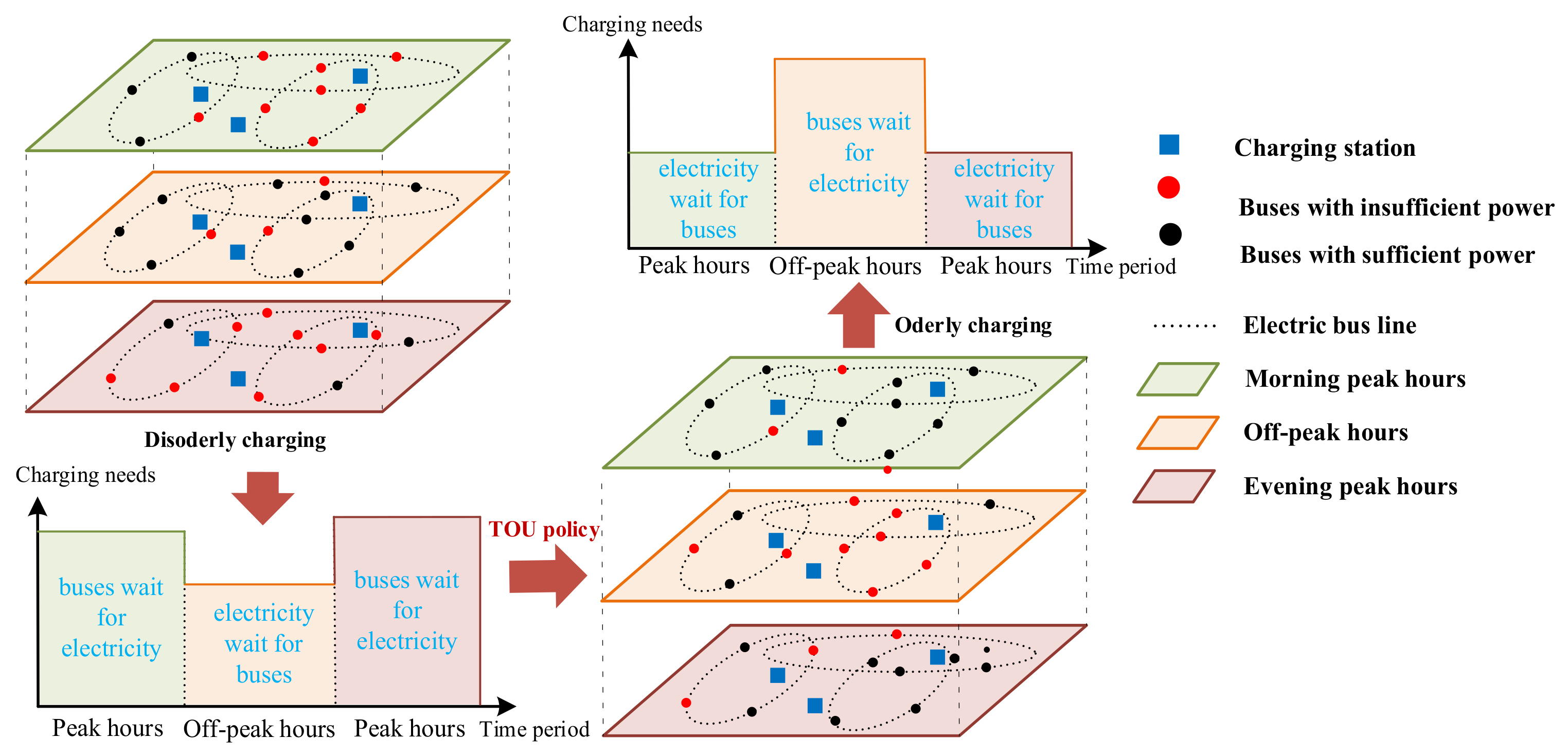
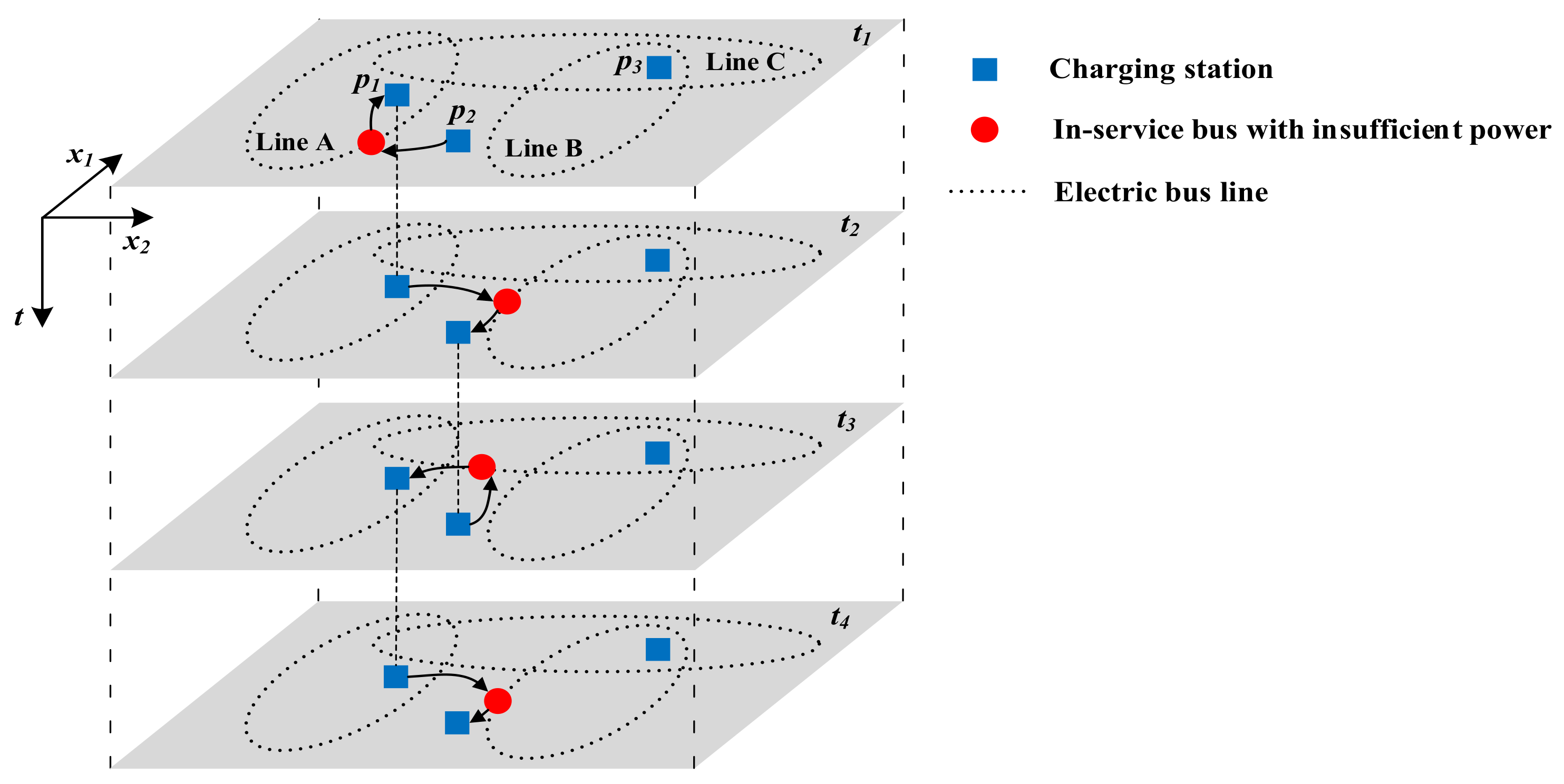
3.1.1. The Bus Replacement Strategy

This paper divides the EB’s operating time horizon $\left[t_s, t_e\right]$ into multiple time slots of equal length. The set of time slots is denoted by $T=\left\{t:t=t_1,t_2,\cdots ,t_{max}\right\}$. Equation (1) determines the number of all time slots according to the start time and end time of the operating hours. During the operation period, each bus departs strictly according to its predetermined departure timetable. The set of operating trips for a bus $\left(n,i\right)$ is represented by $\left\{l:l=1,2,\cdots ,L_{n,i}\right\}$, where $L_{n,i}$ represents its last trip during daytime operation. The set of bus stops along the line $i$ is denoted by $\left\{j:j=1,2,\cdots ,J_n\right\}$, where $J_n$ represents the maximum number of bus stops on line $i$. Under bus replacement management, the bus company needs to dispatch standby buses to designated stops to take over in-service buses with insufficient electricity power. If the standby bus arrives too early, it will cause unnecessary waste of vehicle resources; if it arrives too late, passengers will have to wait too long and have a bad ride experience. A penalty factor, $c_2$, is introduced to ensure standby buses arrive as “on time” as possible. The time penalty for bus arrival is shown in Equation (2), where $k_{n,i,l,j}$ represents the period when the bus arrives at different bus stops, and it can be computed by Equation (3). After replacement, in-service buses are required to return to nearby charging stations for recharging, as defined by Equation (4). Equation (5) represents the service radius constraint for the charging stations.

$$\left|T\right|=int\lceil \left(t_e-t_s\right)/\Delta \rceil ,$$

(1)

$${\omega }_{n,i,l,j}^{p,k,t}=\left|\left[t-\left(k_{n,i,l,j}-1\right)\right]\right|{\alpha }_{n,i,l,j}^{p,k,t},\forall n\in N,i\in \left\{1,2,\cdots ,I_n\right\},l\in \left\{1,2,\cdots ,L_{n,i}\right\},j\in \left\{1,2,\cdots ,J_n\right\}, p\in P,k\in K,t\in T$$

(2)

$$k_{n,i,l,j}=int\lceil t_{n,i,l}+l_{n,j}/v\rceil ,\forall n\in N,i\in \left\{1,2,\cdots ,I_n\right\},l\in \left\{1,2,\cdots ,L_{n,i}\right\},j\in \left\{1,2,\cdots ,J_n\right\}$$

(3)

$${\displaystyle \sum }_{p\in P}{\beta }_{n,i,l,j}^{p,k,t+1}={\displaystyle \sum }_{p\in P}{\alpha }_{n,i,l,j}^{p,k,t},\forall n\in N,i\in \left\{1,2,\cdots ,I_n\right\},l\in \left\{1,2,\cdots ,L_{n,i}\right\},j\in \left\{1,2,\cdots ,J_n\right\},t\in \left\{1,2,\cdots ,T_{max}-1\right\}$$

(4)

$$l_{i,j}^p{\beta }_{n,i,l,j}^{p,k,t}\le {\beta }_{n,i,l,j}^{p,k,t}{R}_p,\forall n\in N,i\in \left\{1,2,\cdots ,I_n\right\},l\in \left\{1,2,\cdots ,L_{n,i}\right\},j\in \left\{1,2,\cdots ,J_n\right\}, p\in P,k\in K,t\in T$$

(5)

In Equation (1), $int\lceil ·\rceil$ represents the ceiling function, $t_s$ and $t_e$ represent the start and end times of daytime operation, respectively, and $\Delta$ denotes the length of each time slot/window. In Equation (2), ${\omega }_{n,i,l,j}^{p,k,t}$ represents the delay/advance time of standby bus $k$ leaving from the charging station $p$ and arriving at bus stop $j$ to take over the in-service bus $\left(n,i,l\right)$. ${\alpha }_{n,i,l,j}^{p,k,t}$ is a binary variable, and ${\alpha }_{n,i,l,j}^{p,k,t}=1$ indicates that standby bus $k$ driving from station $p$ will replace bus $\left(n,i,l\right)$ in time slot $t$; otherwise, ${\alpha }_{n,i,l,j}^{p,k,t}=0$. Please note that the notation bus $\left(n,i,l\right)$ refers to the $i^{th}$ bus on line $n$, which is currently executing its $l^{th}$ driving task. In Equation (3), $t_{n,i,l}$ represents the departure time of bus $\left(n,i,l\right)$, $l_{n,j}$ represents the distance from the starting bus stop to the $j^{th}$ stop on line $n$, and $v$ is the average driving speed of EBs. In Equation (4), ${\beta }_{n,i,l,j}^{p,k,t}$ is a binary variable, and ${\beta }_{n,i,l,j}^{p,k,t}=1$ indicates that the in-service bus $\left(n,i,l\right)$ will proceed to charging station $p$ after being replaced by the $k^{th}$ standby bus in time slot $t$; otherwise, ${\beta }_{n,i,l,j}^{p,k,t}=0$. In Equation (5), $l_{n,j}^p$ represents the distance between the $j^{th}$ stop on line $i$ and the charging station $p$, and $R_p$ denotes the service radius of the charging station $p$.

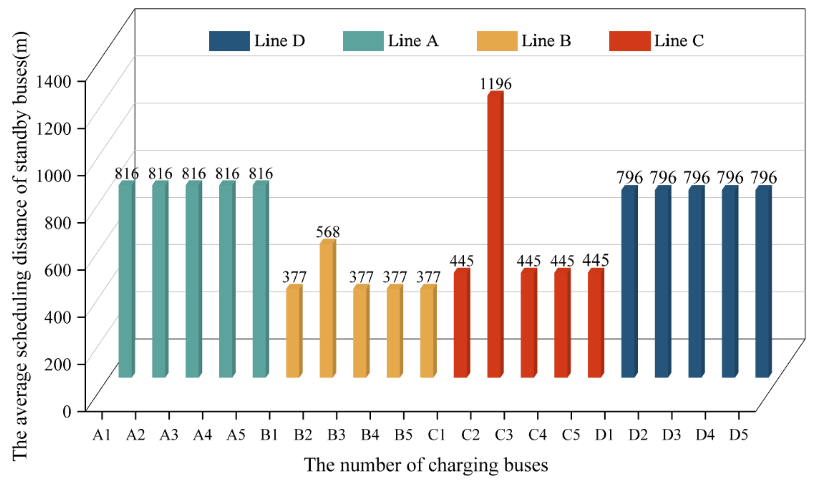
3.1.2. Scheduling Optimization for Standby Buses

Based on the aforementioned bus replacement management approach, standby buses are dynamically assigned between multiple charging stations and scheduled bus stops on different routes. The dispatching scheme for standby buses is formulated as Equations (8) and (9). We enforce the regulation that the replaced bus must return to a nearby charging station within the current time window after completing the replacement task, as specified by Equations (6) and (7). Standby buses that are not engaged in replacement tasks will remain at the current charging station, ready for deployment, as shown in Equation (10). Equation (11) imposes the constraint that each standby bus can only serve one in-service charging bus during a given time slot.

$${{\displaystyle \sum }}_{p\in P}{\tau }^{p,k,t}=1,\forall k\in K,t\in T,$$

(6)

$${\displaystyle \sum }_{p\in P}{\displaystyle \sum }_{t\in T}{\tau }^{p,k,t}=K_{max},\forall k\in K$$

(7)

$${\tau }^{p,k,t}={\tau }^{p,k,t-1}, if {\displaystyle \sum }_{n\in N}{\displaystyle \sum }_{i=1}^{I_n}{\displaystyle \sum }_{l=1}^{L_{n,i}}{\displaystyle \sum }_{j=1}^{J_n}{\alpha }_{n,i,l,j}^{p,k,t}+{\displaystyle \sum }_{n\in N}{\displaystyle \sum }_{i=1}^{I_n}{\displaystyle \sum }_{l=1}^{L_{n,i}}{\displaystyle \sum }_{j=1}^{J_n}{\beta }_{n,i,l,j}^{p,k,t}=0, \forall p\in P,k\in K,t\in \left\{2,3,\cdots ,T_{max}\right\}$$

(8)

$${\displaystyle \sum }_{n\in N}{\displaystyle \sum }_{i=1}^{I_n}{\displaystyle \sum }_{l=1}^{L_{n,i}}{\displaystyle \sum }_{j=1}^{J_n}{\alpha }_{n,i,l,j}^{p,k,t}\le {\tau }^{p,k,t}, \forall p\in P,k\in K,t\in T$$

(9)

$${\displaystyle \sum }_{n\in N}{\displaystyle \sum }_{i=1}^{I_n}{\displaystyle \sum }_{l=1}^{L_{n,i}}{\displaystyle \sum }_{j=1}^{J_n}{\beta }_{n,i,l,j}^{p,k,t}\le {\tau }^{p,k,t}, \forall p\in P,k\in K,t\in T$$

(10)

$${\displaystyle \sum }_{n\in N}{\displaystyle \sum }_{i=1}^{I_n}{\displaystyle \sum }_{l=1}^{L_{n,i}}{\displaystyle \sum }_{j=1}^{J_n}{\alpha }_{n,i,l,j}^{p,k,t}+{\displaystyle \sum }_{n\in N}{\displaystyle \sum }_{i=1}^{I_n}{\displaystyle \sum }_{l=1}^{L_{n,i}}{\displaystyle \sum }_{j=1}^{J_n}{\beta }_{n,i,l,j}^{p,k,t}\le 1, \forall p\in P,k\in K,t\in T$$

(11)

In Equation (6), ${\tau }^{p,k,t}$ is a binary variable, and ${\tau }^{p,k,t}=1$ denotes that standby bus $k$ is located at charging station $p$ during time window $t$; otherwise, ${\tau }^{p,k,t}=0$. In Equation (7), $K_{max}$ represents the number of available standby buses.

3.1.3. Updating the Remaining Battery Energy for In-Service Buses

Equation (12) is utilized to compute the remaining power of buses at the initiation of their first trip after departing from depots. Subsequently, Equation (13) updates the remaining power of buses when they embark on the next service trip. For an electric bus (EB), a service trip encompasses the process of departing from the initial stop, travelling to the terminal, and returning to the departure stop. Notably, the battery power of in-service buses is influenced by the bus replacement strategy. Equation (14) calculates the remaining power of an in-service bus in situations where no replacement occurs during its current trip. Conversely, if replacement does take place, its remaining power is exchanged with that of the corresponding standby bus, as described in Equation (15). The power fluctuation of the on-board battery during operation is represented by the state of charge (SOC), which is computed according to the method presented in Equation (16). To mitigate battery depreciation and prevent over-discharge, a safety threshold [$S_{min}$, $S_{max}$] is defined for battery SOC during scheduling, as expressed in Equation (17). The upper and lower bounds of SOC (%) are denoted by $S_{min}$ and $S_{max}$, respectively.

$$E_{n,i,1,1}=E_0-F_{n,i},\forall n\in N,i\in \left\{1,2,\cdots ,I_n\right\},$$

(12)

$$E_{n,i,l+1,1}=E_{n,i,l,J_i},\forall n\in N,i\in \left\{1,2,\cdots ,I_n\right\},l\in \left\{1,2,\cdots ,L_{n,i}-1\right\}$$

(13)

$${\tau }^{p,k,t}={\tau }^{p,k,t-1}, if {\displaystyle \sum }_{n\in N}{\displaystyle \sum }_{i=1}^{I_n}{\displaystyle \sum }_{l=1}^{L_{n,i}}{\displaystyle \sum }_{j=1}^{J_n}{\alpha }_{n,i,l,j}^{p,k,t}+{\displaystyle \sum }_{n\in N}{\displaystyle \sum }_{i=1}^{I_n}{\displaystyle \sum }_{l=1}^{L_{n,i}}{\displaystyle \sum }_{j=1}^{J_n}{\beta }_{n,i,l,j}^{p,k,t}=0, \forall p\in P,k\in K,t\in \left\{2,3,\cdots ,T_{max}\right\}$$

(14)

$$E_{n,i,l,j}=G^{p,k,t}-\rho l_{n,j}^p, if {\alpha }_{n,i,l,j}^{p,k,t}=1,\forall n\in N,i\in \left\{1,2,\cdots ,I_n\right\},l\in \left\{1,2,\cdots ,L_{n,i}\right\},j\in \left\{1,2,\cdots ,J_n\right\}, p\in P,k\in K,t\in T$$

(15)

$$S_{n,i,l,j}=E_{n,i,l,j}/E_0\times 100\%,\forall n\in N,i\in \left\{1,2,\cdots ,I_n\right\},l\in \left\{1,2,\cdots ,L_{n,i}\right\},j\in \left\{1,2,\cdots ,J_n\right\}$$

(16)

$$S_{min}\le S_{n,i,l,j}\le S_{max},\forall n\in N,i\in \left\{1,2,\cdots ,I_n\right\},l\in \left\{1,2,\cdots ,L_{n,i}\right\},j\in \left\{1,2,\cdots ,J_n\right\}$$

(17)

In Equation (12), $E_0$ denotes the battery capacity, $F_{n,i}$ represents the average energy consumption for bus $\left(n,i\right)$ driving from the depot to its starting bus stop, and $E_{n,i,1,1}$ represents the initial power of bus $\left(n,i\right)$ when it begins to perform the first trip. In Equation (13), $E_{n,i,l,1}$ represents the initial power of bus $\left(n,i\right)$ when it begins to perform the $l^{th}$ trip. In Equation (14), $E_{n,i,l,j}$ represents the remaining power of bus $\left(n,i,l\right)$ when it arrives at the $j^{th}$ bus stop, and $e_{n,j}$ represents the average energy consumption for a bus driving from the starting stop to the $j^{th}$ stop. In Equation (15), $G^{p,k,t}$ represents the remaining power of standby bus $k$ that stayed at charging station $p$ in time window $t$. $\rho$ denotes the energy consumption rate of EBs per unit distance. In Equation (16), $S_{n,i,l,j}$ represents the state of charge (SOC value) of bus $\left(n,i,l\right)$ when it arrives at the $j^{th}$ bus stop.

3.1.4. Updating the Remaining Battery Energy for Standby Buses

When a standby bus remains at a charging station without replacing other buses, its remaining power is updated based on the duration of charging, as presented in Equation (18). However, if the standby bus does execute a replacement task, its remaining power will be exchanged with that of the in-service bus being replaced, as indicated in Equation (19). Similarly, the state of charge (SOC) value of standby buses should also be maintained within a specific safe threshold, as depicted in Equations (20) and (21).

$$G^{p,k,t}=E_{n,i,l,j-1}-e_{n,j}-\rho l_{n,j}^p, if {\beta }_{n,i,l,j}^{p,k,t}=1,\forall n\in N,i\in \left\{1,2,\cdots ,I_n\right\},l\in \left\{1,2,\cdots ,L_{n,i}\right\},j\in \left\{1,2,\cdots ,J_n\right\}, p\in P,k\in K,t\in T$$

(18)

$$G^{p,k,t}=G^{p,k,t-1}+q^{p,k,t},if {\displaystyle \sum }_{n\in N}{\displaystyle \sum }_{i=1}^{I_n}{\displaystyle \sum }_{l=1}^{L_{n,i}}{\displaystyle \sum }_{j=1}^{J_n}{\beta }_{n,i,l,j}^{p,k,t}=0, \forall p\in P,k\in K,t\in \left\{2,3,\cdots ,T_{max}\right\}$$

(19)

$$S^{p,k,t}=G^{p,k,t}/E_0\times 100\%, \forall p\in P,k\in K,t\in T$$

(20)

$$S_{min}\le S^{p,k,t}\le S_{max}, \forall p\in P,k\in K,t\in T$$

(21)

In Equation (19), $q^{p,k,t}$ denotes the energy replenished by standby bus $k$ at charging station $p$ within the time slot $t$. In Equation (20), $S^{p,k,t}$ represents the SOC value of standby bus $k$ at charging station $p$ within the time slot $t$.

3.1.5. Charging Behaviors of Standby Buses under Time-of-Use Electricity Price Policy

The study specifies that the unit charging time of standby vehicles is equivalent to the duration of a time window. Standby buses can charge continuously in multiple time windows to attain the required amount of electricity. Equation (22) represents the energy acquired by a standby bus during a single charging time slot. Importantly, vehicles can only commence charging upon arrival at a charging station, as presented in Equation (23). Equations (24) and (25) impose restrictions on standby buses, prohibiting them from charging while entering or leaving the charging station. Additionally, Equation (26) indicates that standby buses have the option of being fully charged overnight.

$$q^{p,k,t}=D·P^{+}·\eta ·Z^{p,k,t}, \forall p\in P,k\in K,t\in T$$

(22)

$$Z^{p,k,t}\le {\tau }^{p,k,t}, \forall p\in P,k\in K,t\in T$$

(23)

$$Z^{p,k,t}\le 1-{\displaystyle \sum }_{n\in N}{\displaystyle \sum }_{i=1}^{I_n}{\displaystyle \sum }_{l=1}^{L_{n,i}}{\displaystyle \sum }_{j=1}^{J_n}{\beta }_{n,i,l,j}^{p,k,t}, \forall p\in P,k\in K,t\in T$$

(24)

$$Z^{p,k,t}\le 1-{\displaystyle \sum }_{n\in N}{\displaystyle \sum }_{i=1}^{I_n}{\displaystyle \sum }_{l=1}^{L_{n,i}}{\displaystyle \sum }_{j=1}^{J_n}{\alpha }_{n,i,l,j}^{p,k,t}, \forall p\in P,k\in K,t\in T$$

(25)

$$G^{p,k,1}=E_0{\tau }^{p,k,1}, \forall p\in P,k\in K$$

(26)

In Equation (22), $\Delta$ denotes the length of each time slot, $P^{+}$ denotes the charging power of each charger, and $\eta$ represents the energy conversion rate of each charger. $Z^{p,k,t}$ is a binary variable, and $Z^{p,k,t}=1$ means that the standby bus $k$ at charging station $p$ will be recharged during the time slot $t$; otherwise, $Z^{p,k,t}=0$.

3.2. Objective Function

The objective function of this model aims to minimize the weighted sum of four costs, as expressed in Equation (27). The first term represents the electricity energy usage cost, encompassing the electricity expenditure during daytime opportunity charging and night top-up charging, as depicted in Equation (28). The second term signifies the dispatching cost of EBs, as given by Equation (29). The third term represents the passenger costs, the time penalty cost incurred when standby buses arrive unpunctually at designated bus stops, as shown in Equation (30). Under the bus replacement strategy, passengers may need to transfer to another bus to complete their journey. Therefore, the fourth cost represents the inconvenience imposed on passengers, resulting in transfer costs. It can also be considered as the subsidy cost borne by the public transportation company for transferring passengers due to schedule inconvenience. This subsidy can be implemented by offering discounts on the next fare for these transfer passengers. Note that the transfer/subsidy cost is quantified using Equation (31). The remaining battery energy of standby buses and in-service buses at the end of the daytime operation is denoted by Equations (32) and (33), respectively. Furthermore, under the time-of-use electricity pricing policy, the unit electricity price is fixed for each time slot, as specified by the local government, as shown in Equation (34). Equations (35) and (36) represent the electricity costs for charging buses during daytime operation and throughout the night, respectively.

$$min \left(D+O+U+H\right)$$

(27)

$$D=D_1+D_2$$

(28)

$$O=c_1{\displaystyle \sum }_{n\in N}{\displaystyle \sum }_{i=1}^{I_n}{\displaystyle \sum }_{l=1}^{L_{n,i}}{\displaystyle \sum }_{j=1}^{J_n}{\displaystyle \sum }_{p\in P}{\displaystyle \sum }_{k\in K}{\displaystyle \sum }_{t\in T}{l}_{n,j}^p\left({\alpha }_{n,i,l,j}^{p,k,t}+{\beta }_{n,i,l,j}^{p,k,t}\right)$$

(29)

$$U=\left\{\begin{array}{c}{c}_{2,1}{\displaystyle {\displaystyle \sum }_{n\in N}}{\displaystyle {\displaystyle \sum }_{i=1}^{I_n}}{\displaystyle {\displaystyle \sum }_{l=1}^{L_{n,i}}}{\displaystyle {\displaystyle \sum }_{j=1}^{J_n}}{\displaystyle {\displaystyle \sum }_{p\in P}}{\displaystyle {\displaystyle \sum }_{k\in K}}{\displaystyle {\displaystyle \sum }_{t\in T}}{\omega }_{n,i,l,j }^{p,k,t}, \mathrm{if} t\ge \left(k_{n,i,l,j}-1\right) \\ c_{2,2}{\displaystyle {\displaystyle \sum }_{n\in N}}{\displaystyle {\displaystyle \sum }_{i=1}^{I_n}}{\displaystyle {\displaystyle \sum }_{l=1}^{L_{n,i}}}{\displaystyle {\displaystyle \sum }_{j=1}^{J_n}}{\displaystyle {\displaystyle \sum }_{p\in P}}{\displaystyle {\displaystyle \sum }_{k\in K}}{\displaystyle {\displaystyle \sum }_{t\in T}}{\omega }_{n,i,l,j}^{p,k,t}, \mathrm{if} t<\left(k_{n,i,l,j}-1\right)\end{array}\right.$$

(30)

$$H=c_3{\displaystyle \sum }_{n\in N}{\displaystyle \sum }_{i=1}^{I_n}{\displaystyle \sum }_{l=1}^{L_{n,i}}{\displaystyle \sum }_{j=1}^{J_n}{\displaystyle \sum }_{p\in P}{\displaystyle \sum }_{k\in K}{\displaystyle \sum }_{t\in T}{\alpha }_{n,i,l,j}^{p,k,t} h_{n,i,l,j}$$

(31)

$$D^k={\displaystyle \sum }_{p\in P}{G}^{p,k,T_{max}}{\tau }^{p,k,T_{max}},k\in K$$

(32)

$$D_{n,i}=E_{n,i,L_{n,i},J_n}-U_{n,i},\forall n\in N,i\in \left\{1,2,\cdots ,I_n\right\}$$

(33)

$${\theta }_t=\left\{\begin{array}{c}{\theta }_l, t\in velley hours\\ {\theta }_g, t\in peak hours\\ {\theta }_p, t\in flat hours\end{array}\right.$$

(34)

$$D_1={\displaystyle \sum }_{p\in P}{\displaystyle \sum }_{k\in K}{\displaystyle \sum }_{t\in T}{\theta }_t{q}^{p,k,t}$$

(35)

$$D_2={\theta }_l({\displaystyle \sum }_{k\in K}{D}^k+{\displaystyle \sum }_{n\in N}{\displaystyle \sum }_{i=1}^{I_n}{D}_{n,i})$$

(36)

In Equation (29), $c_1$ represents the dispatch cost per unit distance for EBs. In Equation (30), $c_{2,1}$ and $c_{2,2}$ represent the penalty cost per unit of time for buses arriving late and early at the takeover locations, respectively. In Equation (31), $c_3$ denotes the unit transfer/subsidy cost per transferred passenger, and $h_{n,i,l,j}$ denotes the average onboard passengers at the $j^{th}$ stop. In Equation (32), $D^k$ denotes the remaining energy of the standby bus at the end of daytime operation. In Equation (33), $E_{n,i,L_{n,i},J_n}$ represents the remaining power of the EB after completing all driving tasks, and $U_{n,i}$ represents the average energy consumption of an EB $\left(n,i\right)$ on the trip from the ending bus stop to the depot. In Equation (34), ${\theta }_l$, ${\theta }_g$, and ${\theta }_p$ represent the unit electricity prices during valley hours, peak hours, and flat hours, respectively, and ${\theta }_t$ is the unit electricity prices within time window $t$.

4. Model Linearization and Solution

The proposed model poses a mixed-integer nonlinear problem (MINLP). The nonlinear constraints primarily include: (i) Equation (2) contains the absolute-value function, while Equations (8), (14), (15), (18), and (19) comprise “if” statements, and (ii) Equation (32) represents the product of multiple binary variables. However, the remaining constraints and objective functions are linear formulas. In this section, we aim to linearize the aforementioned nonlinear formulas while preserving the original equations’ logic and meaning.

Equation (2) contains the absolute-value function that can be linearized by introducing binary variables ${\theta }_{n,i,l,j}^{p,k,t}$ and ${\vartheta }_{n,i,l,j}^{p,k,t}$, as shown in Equations (37)–(39). Here, ${\theta }_{n,i,l,j}^{p,k,t}$ is a binary variable, and ${\theta }_{n,i,l,j}^{p,k,t}=1$ means that the in-service bus $\left(n,i,l\right)$ arrives at the designated stop $j$ first and waits to be replaced by standby bus $k$ departing from charging station $p$ in time slot $t$; otherwise, ${\theta }_{n,i,l,j}^{p,k,t}=0$. ${\vartheta }_{n,i,l,j}^{p,k,t}$ is a binary variable, and ${\vartheta }_{n,i,l,j}^{p,k,t}=1$ means that standby bus $k$ departing from charging station $p$ arrives at the designated stop $j$ in advance to take over the in-service bus $\left(n,i,l\right)$ in time slot $t$.

$${\omega }_{n,i,l,j}^{p,k,t}\ge 0,\forall n\in N,i\in \left\{1,2,\cdots ,I_n\right\},l\in \left\{1,2,\cdots ,L_{n,i}\right\},j\in \left\{1,2,\cdots ,J_n\right\},p\in P,k\in K,t\in T$$

(37)

$${\theta }_{n,i,l,j}^{p,k,t}+{\vartheta }_{n,i,l,j}^{p,k,t}={\alpha }_{n,i,l,j}^{p,k,t},\forall n\in N,i\in \left\{1,2,\cdots ,I_n\right\},l\in \left\{1,2,\cdots ,L_{n,i}\right\},j\in \left\{1,2,\cdots ,J_n\right\},p\in P,k\in K,t\in T$$

(38)

$${\omega }_{n,i,l,j}^{p,k,t}=\left[t-\left(k_{n,i,l,j}-1\right)\right]{\theta }_{n,i,l,j}^{p,k,t}+\left[\left(k_{n,i,l,j}-1\right)-t\right]\left(1-{\vartheta }_{n,i,l,j}^{p,k,t}\right),\forall n\in N,i\in \left\{1,2,\cdots ,I_n\right\},l\in \left\{1,2,\cdots ,L_{n,i}\right\},j\in \left\{1,2,\cdots ,J_n\right\},p\in P,k\in K,t\in T$$

(39)

Equation (8) contains the “if” statement, which is nonlinear. To linearize this equation, we can introduce a large positive number to relax the constraint, as shown in Equations (40) and (41):

$${\tau }^{p,k,t}-{\tau }^{p,k,t-1}\le M{\displaystyle \sum }_{n\in N}{\displaystyle \sum }_{i=1}^{I_n}{\displaystyle \sum }_{l=1}^{L_{n,i}}{\displaystyle \sum }_{j=1}^{J_n}{\alpha }_{n,i,l,j}^{p,k,t}+M{\displaystyle \sum }_{n\in N}{\displaystyle \sum }_{i=1}^{I_n}{\displaystyle \sum }_{l=1}^{L_{n,i}}{\displaystyle \sum }_{j=1}^{J_n}{\beta }_{n,i,l,j}^{p,k,t}, \forall p\in P,k\in K,t\in \left\{2,3,\cdots ,T_{max}\right\}$$

(40)

$$-M{\displaystyle \sum }_{n\in N}{\displaystyle \sum }_{i=1}^{I_n}{\displaystyle \sum }_{l=1}^{L_{n,i}}{\displaystyle \sum }_{j=1}^{J_n}{\alpha }_{n,i,l,j}^{p,k,t}-M{\displaystyle \sum }_{n\in N}{\displaystyle \sum }_{i=1}^{I_n}{\displaystyle \sum }_{l=1}^{L_{n,i}}{\displaystyle \sum }_{j=1}^{J_n}{\beta }_{n,i,l,j}^{p,k,t}\le {\tau }^{p,k,t}-{\tau }^{p,k,t-1}, \forall p\in P,k\in K,t\in \left\{2,3,\cdots ,T_{max}\right\}$$

(41)

Similarly, Equations (14), (15), (18), and (19) can be linearized as Equations (42)–(43), (44)–(45), (46)–(47), and (48)–(49), respectively:

$$E_{n,i,l,j}-\left(E_{n,i,l,j-1}-e_{i,j}\right)\le M{\displaystyle \sum }_{p\in P}{\displaystyle \sum }_{k\in K}{\displaystyle \sum }_{t\in T}{\alpha }_{n,i,l,j}^{p,k,t},\forall n\in N,i\in \left\{1,2,\cdots ,I_n\right\},l\in \left\{1,2,\cdots ,L_{n,i}\right\},j\in \left\{1,2,\cdots ,J_n\right\}$$

(42)

$$-M{\displaystyle \sum }_{p\in P}{\displaystyle \sum }_{k\in K}{\displaystyle \sum }_{t\in T}{\alpha }_{n,i,l,j}^{p,k,t}\le E_{n,i,l,j}-\left(E_{n,i,l,j-1}-e_{i,j}\right),\forall n\in N,i\in \left\{1,2,\cdots ,I_n\right\},l\in \left\{1,2,\cdots ,L_{n,i}\right\},j\in \left\{1,2,\cdots ,J_n\right\}$$

(43)

$$E_{n,i,l,j}-\left(G^{p,k,t}-\rho l_{n,j}^p\right)\le M\left(1-{\alpha }_{n,i,l,j}^{p,k,t}\right),\forall n\in N,i\in \left\{1,2,\cdots ,I_n\right\},l\in \left\{1,2,\cdots ,L_{n,i}\right\},j\in \left\{1,2,\cdots ,J_n\right\},\forall p\in P,k\in K,t\in T$$

(44)

$$M\left(1-{\alpha }_{n,i,l,j}^{p,k,t}\right)\le E_{n,i,l,j}-\left(G^{p,k,t}-\rho l_{n,j}^p\right),\forall n\in N,i\in \left\{1,2,\cdots ,I_n\right\},l\in \left\{1,2,\cdots ,L_{n,i}\right\},j\in \left\{1,2,\cdots ,J_n\right\},\forall p\in P,k\in K,t\in T$$

(45)

$$G^{p,k,t}-\left(E_{n,i,l,j-1}-e_{n,j}-\rho l_{n,j}^p\right)\le M\left(1-{\beta }_{n,i,l,j}^{p,k,t}\right),\forall n\in N,i\in \left\{1,2,\cdots ,I_n\right\},l\in \left\{1,2,\cdots ,L_{n,i}\right\},j\in \left\{1,2,\cdots ,J_n\right\},p\in P,k\in K,t\in T$$

(46)

$$-M\left(1-{\beta }_{n,i,l,j}^{p,k,t}\right)\le G^{p,k,t}-\left(E_{n,i,l,j-1}-e_{n,j}-\rho l_{n,j}^p\right),\forall n\in N,i\in \left\{1,2,\cdots ,I_n\right\},l\in \left\{1,2,\cdots ,L_{n,i}\right\},j\in \left\{1,2,\cdots ,J_n\right\},p\in P,k\in K,t\in T$$

(47)

$$G^{p,k,t}-\left(G^{p,k,t-1}+q^{p,k,t}\right)\le M{\displaystyle \sum }_{n\in N}{\displaystyle \sum }_{i=1}^{I_n}{\displaystyle \sum }_{l=1}^{L_{n,i}}{\displaystyle \sum }_{j=1}^{J_n}{\beta }_{n,i,l,j}^{p,k,t}, \forall p\in P,k\in K,t\in \left\{2,3,\cdots ,T_{max}\right\}$$

(48)

$$-M{\displaystyle \sum }_{n\in N}{\displaystyle \sum }_{i=1}^{I_n}{\displaystyle \sum }_{l=1}^{L_{n,i}}{\displaystyle \sum }_{j=1}^{J_n}{\beta }_{n,i,l,j}^{p,k,t}\le G^{p,k,t}-\left(G^{p,k,t-1}+q^{p,k,t}\right), \forall p\in P,k\in K,t\in \left\{2,3,\cdots ,T_{max}\right\}$$

(49)

In constraint (32), $G^{p,k,T_{max}}$ and ${\tau }^{p,k,T_{max}}$ are binary variables. The multiplication of two variables is nonlinear, and to linearize it, we can introduce the real variable $Q^{p,k,T_{max}}$ and the large positive number $M$, as presented in Equations (50)–(53). When ${\tau }^{p,k,T_{max}}=1$, $Q^{p,k,T_{max}}=G^{p,k,T_{max}}$ holds true; otherwise, $Q^{p,k,T_{max}}=0$ is satisfied. This representation is equivalent to Equation (32). Here, $Q^{p,k,T_{max}}$ denotes the remaining battery power of standby bus $k$ at charging station $p$ when daytime operation ends, i.e., at time $t=T_{max}$.

$$Q^{p,k,T_{max}}\le G^{p,k,T_{max}}+M\left(1-{\tau }^{p,k,T_{max}}\right), \forall p\in P,k\in K$$

(50)

$$G^{p,k,T_{max}}-M\left(1-{\tau }^{p,k,T_{max}}\right)\le Q^{p,k,T_{max}}, \forall p\in P,k\in K$$

(51)

$$0\le Q^{p,k,T_{max}}\le M{\tau }^{p,k,T_{max}}, \forall p\in P,k\in K$$

(52)

$$D^k={\displaystyle \sum }_{p\in P}{Q}^{p,k,T_{max}},\forall k\in K$$

(53)

After the linearization process, the proposed model is transformed into a standard mixed-integer linear programming problem (MILP), formulated as follows:

The objective function: $min \left(D+O+U\right)$.

Decision variables: ${\alpha }_{n,i,l,j}^{p,k,t}$, ${\beta }_{n,i,l,j}^{p,k,t}$, $Z^{p,k,t}$.

Constraints: Equations (3)–(7), (16), (17), (20)–(31), and (33)–(53).

For the case study, we implement the model using a mathematical programming language (AMPL) and utilize the GUROBI MILP solver to obtain the optimal solution.

5. Model Validation

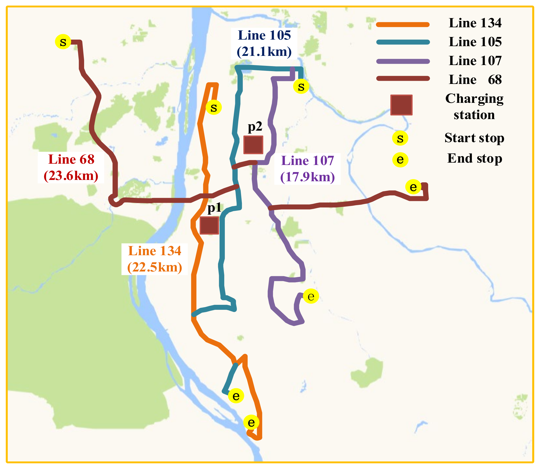
5.1. Parameter Inputs

A case study was conducted in Changsha, China, which focused on four bus lines: Line 134, Line 105, Line 107, and Line 23, referred to as “Line A” to “Line D”, respectively. The study period was during the peak hour from 6:00 to 7:00. According to the predetermined timetable, each line will have a total of five buses departing during the study period. Each bus is numbered based on its departure order. In this context, a service trip is defined as a process that begins from the departure station, travels to the terminal, and then returns to the departure station. Therefore, we define $J_i\left(i\in I\right)$ as the sum of all stops along a loop trip, where $J_A=$102, $J_B=$82, $J_C=$74, and $J_D=$ 68. To ensure that standby vehicles arrive on time during the optimal period, we set the penalty coefficients for early and late arrivals to very large positive integers. It is worth noting that for further investigation into the impact of standby vehicle arrival times on the charging schedule, the values of the unit time costs for early and late arrivals can be referenced from [52,53]. The parameter inputs for this case study are summarized in

Table 1. The parameter inputs.

The average driving speed of EBs, $v$/[km/h]	25	Starting time of bus operation hours, $t_s$	6:00
The dispatch cost per unit distance for EBs, $c_1$/[yuan/km]	1	Ending time of bus operation hours, $t_e$	22:30
The upper bounds of SOC, $S_{min}$	0.2	The length of unit time window, $\Delta$/[h]	1
The lower bounds of SOC, $S_{max}$	1	Battery capacity, $E_0$/[kW·h]	200
The penalty cost per unit time for buses arriving early (or late) at the takeover locations, $c_{\mathbf{2},\mathbf{1}}$ (or $c_{\mathbf{2},\mathbf{2}}$)/[yuan/h]	250/500	Service radius of charging station, $R_p$/[km]	1.5
Unit transfer/subsidy cost, $c_3$/[yuan/passenger]		0.5
The energy consumption rate per unit distance, $\rho$/[kW·h/km]	1.2	A large position, $M$	100,000
The energy conversion rate of each charger, $\eta$/[%]	90	The charging power of each charger, $P^{+}$/[kW·h]	70
Peak hours	6:00~12:00, 6:00~21:00
Flat hours	12:00~17:00
Valley hours	21:00~24:00, 0:00~6:00
Unit electricity prices during peak hours, ${\theta }_g$/[yuan/kW·h]	1
Unit electricity prices during flat hours, ${\theta }_p$/[yuan/kW·h]	0.6
Unit electricity prices during valley hours, ${\theta }_l$/[yaun/kW·h]	0.3

. The distribution of charging stations and bus lines is illustrated in Figure 3.

The proposed model was implemented using AMPL and comprised 4423 variables and 9850 constraints. The laptop used for solving the model has the Win10 64-bit operating system, an 11th Gen Intel(R) Core(TM) i5-11300H @3.10 GHz 2.61 GHz processor, and 16 GB memory. The optimization results were obtained in approximately 3 h and 43 min. Considering the static nature of the problem under investigation in this paper, the authors assumed that longer solution times are deemed acceptable in pursuit of achieving the optimal solution. However, if there arises a requirement to expedite the solution process, one could opt for obtaining suboptimal solutions by imposing a predefined time limit on the optimization procedure. Moreover, intelligent algorithms, such as genetic algorithms or particle swarm optimization, can be harnessed to acquire feasible solutions.

5.2. Results’ Analysis and Evaluation

The results of various costs based on the aforementioned parameters are summarized in

Table 2. The results of various costs.

Bus Line	Total Scheduling Distance (km)	Punishment for Unpunctual Arrival (Yuan)	Electricity Cost in Peak Hours (Yuan)	Electricity Cost in Flat Hours (Yuan)	Electricity Cost in Valley Hours (Yuan)	Total Electricity Cost (Yuan)	Transfer/ Subsidy Cost (Yuan)	Total Cost (Yuan)
A	8.16	0	0	0	279.64	279.64	35.5	323.3
B	4.653	0	0	0	266.31	266.31	40.12	311.07
C	11.263	0	0	37.8	229.60	267.40	41.53	320.21
D	12.736	0	0	0	323.96	323.96	35.86	372.57
Total	36.812	0	0	37.8	1099.53	1137.33	153.01	1327.16

. Additionally, Figure 4 presents the scheduling distance for standby buses while travelling between charging stations and designated bus stops, and Figure 5 displays the number of bus replacements and the charging times of standby buses.

From Table 2, several key observations can be summarized:

(i) The electricity cost for charging buses constituted over 90% of the total cost. During peak hours, flat hours, and valley hours, the electricity costs amounted to 0 yuan, 37.8 yuan, and 1099.53 yuan, respectively, accounting for 0%, 3.32%, and 96.68% of the total electricity cost. This highlights the model’s effectiveness in achieving cost-efficient charging practices.

(ii) The timely arrival of standby vehicles at designated bus stops is ensured due to the high penalties associated with early or late arrivals per unit time. This ensures the turnover efficiency of standby buses and the operational reliability, particularly punctuality, of in-service buses.

(iii) The transfer/subsidy cost associated with passengers’ transfers constituted approximately 11.53% of the total expenditure. The forthcoming model comparison will further investigate the transfer/subsidy costs incurred under the bus replacement strategy and the concurrent reduction in electricity costs resulting from the implementation of TOU policies.

(iv) The total scheduling cost of standby vehicles was minimal, representing only 3.14% of the total cost. Constrained by the service radius of the charging station, standby vehicles undergo short dispatching distances, ranging from 377 m to 1196 m, and arrive at designated bus stops within brief durations, as depicted in Figure 4.

As depicted in Figure 5, the analysis revealed the following observations:

(i) The total number of bus replacements reached 23 occurrences, with a peak utilization rate of 4 vehicles per hour for standby buses. On average, each of the 4 standby buses provided service for 5.7 instances per vehicle, accounting for 40.7% of the maximum daily service capacity. These findings highlight the remarkable utilization rates of standby buses, suggesting that a modest number of such buses can efficiently meet the considerable demands for replacements.

(ii) It was observed that only one standby bus was involved in a charging event, indicating that standby buses can be utilized as energy storage to provide power for operating buses during daytime hours.

According to bus company regulations, each bus route is normally equipped with 1–2 standby buses, intended to address contingencies, such as power failures during bus operations or adverse weather conditions, including heavy rain or snow. Based on the case study findings, all replacement assignments were efficiently handled by deploying the existing standby buses across lines A, B, C, and D, rendering additional investments in standby buses unnecessary.

5.3. Model Comparison

In this study, we evaluated the charging scheduling efficiency of the proposed decision methods, which included bus charging scheduling under bus replacement strategies considering the TOU electricity policy, denoted as BRS-TOU, and bus charging scheduling under bus replacement strategies without the TOU policy, denoted as BRS. For comparison purposes, we also considered two additional methods: regular charging scheduling considering the TOU policy, denoted as RCS-TOU, and regular charging scheduling without the TOU policy, denoted as RCS.

It is important to note that regular charging scheduling refers to the practice of vehicles driving into a nearby charging station for recharging, as long as they are not serving passengers. The four methods mentioned above were compared to assess their effectiveness in optimizing the charging schedules for EBs in the context of bus replacement strategies and the TOU electricity pricing policy.

Figure 6 presents a schematic diagram illustrating the charging power and the corresponding time-of-use electricity prices under the four schemes. The charging plans under these methods demonstrated notable differences. The proposed scheme, BRS-TOU, exhibited the most favorable charging benefits, as only one standby bus was charged during the daytime flat period. This implies that standby buses effectively balanced the charging requirements of vehicles on different lines through dynamic bus replacement, thereby reducing the overall daytime charging load.

Conversely, in the absence of considering the time-of-use electricity price, the probability of buses charging randomly during the day increased, resulting in a higher charging demand and significant fluctuations in charging power during peak periods. This highlights the importance of incorporating the TOU policy in the charging scheduling optimization to achieve more efficient and cost-effective charging plans for EBs.

Figure 7 presents the electricity cost of charging buses and the amount of recharged power under different methods. The results show that the proposed BRS-TOU method achieved the lowest electricity cost, with 98% of the charging process concentrated during the night valley period. When compared to the BRS method, the BRS-TOU method increased the amount of recharged power during the night valley period by 11%, while reducing it by 2% and 9% during the daytime peak and flat periods, respectively. Under TOU electricity pricing, the standby bus tended to charge during periods of low electricity demand, whereas the in-service bus preferred to maintain vehicles at a low level of SOC when finishing daytime operations. This optimization led to a total decrease of 13% in electricity costs, indicating the high economic efficiency of the optimized charging schemes under the time-of-use electricity pricing strategy.

Furthermore, compared with the RCS-TOU method, the bus replacement strategy effectively utilized standby buses as energy storage devices to supplement the energy power of in-service buses, resulting in a 21% reduction in daytime electricity demand and a total electricity cost reduction of 25.27%. This highlights the effectiveness of the bus replacement strategy proposed in this paper. In comparison to the RCS method, the BRS-TOU method achieved a remarkable 33.29% reduction in total electricity costs. This demonstrates the synergistic effect of the bus replacement strategy and time-of-use policy in dynamically allocating electricity power to operating buses on multiple lines, jointly reducing the overall system cost. Specifically, standby buses, acting as energy storage devices, can respond to the time-of-use (TOU) pricing strategies by storing energy during off-peak periods. Then, through the bus replacement strategy, standby buses can serve as mobile power sources, flexibly scheduled across multiple routes, thereby utilizing the energy stored during off-peak periods for charging needs during peak periods.

Additionally, in comparison to the RCS-TOU strategy, the proposed model resulted in a transfer/subsidy cost of 153.01 yuan, coupled with a substantial reduction in electricity expenses amounting to 348.61 yuan. These findings indicate that the considerable savings achieved in electricity costs effectively offset the potential transfer/subsidy costs incurred for transferred passengers.

6. Conclusions

This paper presented an innovative bus replacement strategy to address the challenges in electric bus charging scheduling. The strategy involves the dynamic dispatch of standby EBs from nearby charging stations to replace in-service buses with insufficient power at designated bus stops. Passengers transfer to the standby buses to complete their journeys, while the replaced buses proceed to the charging station and become “standby buses” after being recharged. This proposed model is capable of dynamically assigning standby buses to different bus lines using bus replacement strategies, resulting in peak shaving and valley filling of the electrical system without compromising on vehicle scheduling efficiency. Although this strategy increases the cost for standby buses and passengers, its effects on reducing the system’s charging costs, improving scheduling efficiency, and balancing the electrical load are more significant, which is sustainable in the long term.

To address this problem effectively, this study first established a model to describe the state of electric bus operations. Then, an electric bus scheduling optimization model was developed under the bus replacement strategy, considering constraints such as time-of-use electricity prices, remaining battery power, and the number of available standby buses. The objective was to minimize the weighted sum of total scheduling and electricity costs. The optimization variables included the dispatch plan of standby buses (i.e., determining the routes from charging stations to specific bus stops), the charging schedule of in-service buses (i.e., identifying the routes from bus stops to charging stations), and the charging plans of each bus at charging stations (i.e., specifying when, where, and how long each bus should be charged).

In the case study, it was revealed that (i) bus replacement strategies can dynamically allocate EBs with different power levels to multiple bus lines, resulting in a substantial 25.27% reduction in charging costs. (ii) When considering the time-of-use pricing policy, the electricity costs were reduced by 33.29% by utilizing standby buses as mobile power sources during daytime hours. Furthermore, it revealed that the substantial savings attained in electricity costs can effectively offset the potential transfer/subsidy costs incurred for transferred passengers. (iii) A modest number of standby buses can efficiently meet the demands for replacements. For example, based on the case study findings, all replacement assignments were efficiently handled by deploying the existing standby buses across lines A, B, C, and D, rendering additional investments in standby buses unnecessary.

During the electrification process of public transportation, the proposed bus replacement strategies offer enhanced flexibility in meeting charging demands across various periods. This approach not only improved the vehicle charging efficiency but also lowered the system’s charging costs, which is crucial for promoting the sustainable development of electric transportation. This paper can be extended in several ways. First, the proposed model solely quantifies the inconvenience of bus replacement to passengers through the time cost associated with transferring, without analyzing the degree of user acceptance of the replacement strategy from the perspective of passenger perception. Therefore, in the next step of our research, we will model users’ travel perceptions from the perspective of user experiences to validate the social application value of the bus replacement strategy. Second, this study aimed to optimize bus charging schedules within the framework of TOU electricity pricing and bus replacement strategies. Building on existing research, we simplified bus scheduling optimization by assuming constant vehicle speeds and energy consumption rates [22,54]. In the next step, by including more bus lines and conducting extensive simulations, the robustness and applicability of the proposed model can be thoroughly tested under various real-world scenarios. Furthermore, this paper utilized a centralized solving algorithm capable of identifying global optimal solutions but at the expense of computational speed [55,56]. Moving forward, we aim to explore advanced optimization algorithms, including decentralized and distributed approaches, to address the optimization challenges more efficiently [57,58].

References

1. Xylia, M.; Leduc, S.; Patrizio, P.; Silveira, S.; Kraxner, F. Developing a dynamic optimization model for electric bus charging infrastructure. Transp. Res. Procedia 2017, 27, 776–783. [Google Scholar] [CrossRef]
2. Hu, X.; Lei, H.; Deng, D.; Bi, Y.; Zhao, J.; Wang, R. A two-stage approach to siting electric bus charging stations considering future-current demand. J. Clean. Prod. 2023, 434, 139962. [Google Scholar] [CrossRef]
3. Bie, Y.; Liu, Y.; Li, S.; Wang, L. HVAC operation planning for electric bus trips based on chance-constrained programming. Energy 2022, 258, 124807. [Google Scholar] [CrossRef]
4. Liu, Z.; Song, Z.; He, Y. Optimal Deployment of Dynamic Wireless Charging Facilities for an Electric Bus System. Transp. Res. Rec. J. Transp. Res. Board 2017, 2647, 100–108. [Google Scholar] [CrossRef]
5. Wang, J.; Rakha, H.A. Modeling fuel consumption of hybrid electric buses: Model development and comparison with conventional buses. Transp. Res. Rec. J. Transp. Res. Board 2016, 2539, 94–102. [Google Scholar] [CrossRef]
6. Lim, L.K.; Ab Muis, Z.; Ho, W.S.; Hashim, H.; Chien, C.B.P. Review of the energy forecasting and scheduling model for electric buses. Energy 2022, 263, 125773. [Google Scholar] [CrossRef]
7. Jiang, M.; Zhang, Y.; Zhang, Y. Optimal electric bus scheduling under travel time uncertainty: A robust model and solution method. J. Adv. Transp. 2021, 2021, 1191443. [Google Scholar] [CrossRef]
8. Lajunen, A. Lifecycle costs and charging requirements of electric buses with different charging methods. J. Clean. Prod. 2018, 172, 56–67. [Google Scholar] [CrossRef]
9. Yan, M.; He, H.; Li, M.; Li, G.; Zhang, X.; Chen, Z. A comprehensive life cycle assessment on dual-source pure electric bus. J. Clean. Prod. 2020, 276, 122702. [Google Scholar] [CrossRef]
10. Chen, Q.; Niu, C.; Tu, R.; Li, T.; Wang, A.; He, D. Cost-effective electric bus resource assignment based on optimized charging and decision robustness. Transp. Res. Part D Transp. Environ. 2023, 118, 103724. [Google Scholar] [CrossRef]
11. Bie, Y.; Cong, Y.; Yang, M.; Wang, L. Coordinated Scheduling of Electric Buses for Multiple Routes Considering Stochastic Travel Times. J. Transp. Eng. Part A Syst. 2023, 149, 4023069. [Google Scholar] [CrossRef]
12. Zhang, A.; Li, T.; Zheng, Y.; Li, X.; Abdullah, M.G.; Dong, C. Mixed electric bus fleet scheduling problem with partial mixed-route and partial recharging. Int. J. Sustain. Transp. 2022, 16, 73–83. [Google Scholar] [CrossRef]
13. Huang, D.; Wang, S. A two-stage stochastic programming model of coordinated electric bus charging scheduling for a hybrid charging scheme. Multimodal Transp. 2022, 1, 100006. [Google Scholar] [CrossRef]
14. Wang, J.; Rakha, H.A. Convex fuel consumption model for diesel and hybrid buses. Transp. Res. Rec. J. Transp. Res. Board 2017, 2647, 50–60. [Google Scholar] [CrossRef]
15. Tang, C.; Li, X.; Ceder, A.; Wang, X. Public transport fleet replacement optimization using multi-type battery-powered electric buses. Transp. Res. Rec. J. Transp. Res. Board 2021, 2675, 1422–1431. [Google Scholar] [CrossRef]
16. Li, L.; Lo, H.K.; Huang, W.; Xiao, F. Mixed bus fleet location-routing-scheduling under range uncertainty. Transp. Res. Part B Methodol. 2021, 146, 155–179. [Google Scholar] [CrossRef]
17. Yao, E.; Liu, T.; Lu, T.; Yang, Y. Optimization of electric vehicle scheduling with multiple vehicle types in public transport. Sustain. Cities Soc. 2020, 52, 101862. [Google Scholar] [CrossRef]
18. Liu, Z.; Song, Z.; He, Y. Economic Analysis of On-Route Fast Charging for Battery Electric Buses: Case Study in Utah. Transp. Res. Rec. J. Transp. Res. Board 2019, 2673, 119–130. [Google Scholar] [CrossRef]
19. Zeng, B.; Wu, W.; Ma, C. Electric bus scheduling and charging infrastructure planning considering bus replacement strategies at charging stations. IEEE Access 2023, 11, 125328–125345. [Google Scholar] [CrossRef]
20. Liu, K.; Gao, H.; Liang, Z.; Zhao, M.; Li, C. Optimal charging strategy for large-scale electric buses considering resource constraints. Transp. Res. Part D Transp. Environ. 2021, 99, 103009. [Google Scholar] [CrossRef]
21. He, Y.; Liu, Z.; Song, Z. Optimal charging scheduling and management for a fast-charging battery electric bus system. Transp. Res. Part E Logist. Transp. Rev. 2020, 142, 102056. [Google Scholar] [CrossRef]
22. Gabriel, N.R.; Martin, K.K.; Haslam, S.J.; Faile, J.C.; Kamens, R.M.; Gheewala, S.H. A comparative life cycle assessment of electric, compressed natural gas, and diesel buses in Thailand. J. Clean. Prod. 2021, 314, 128013. [Google Scholar] [CrossRef]
23. An, K.; Jing, W.; Kim, I. Battery-swapping facility planning for electric buses with local charging systems. Int. J. Sustain. Transp. 2020, 14, 489–502. [Google Scholar] [CrossRef]
24. An, K. Battery electric bus infrastructure planning under demand uncertainty. Transp. Res. Part C Emerg. Technol. 2020, 111, 572–587. [Google Scholar] [CrossRef]
25. Bie, Y.; Ji, J.; Wang, X.; Qu, X. Optimization of electric bus scheduling considering stochastic volatilities in trip travel time and energy consumption. Comput. Aided Civ. Infrastruct. Eng. 2021, 36, 1530–1548. [Google Scholar] [CrossRef]
26. Liu, T.; Ceder, A.A. Battery-electric transit vehicle scheduling with optimal number of stationary chargers. Transp. Res. Part C Emerg. Technol. 2020, 114, 118–139. [Google Scholar] [CrossRef]
27. Ma, X.; Miao, R.; Wu, X.; Liu, X. Examining influential factors on the energy consumption of electric and diesel buses: A data-driven analysis of large-scale public transit network in Beijing. Energy 2021, 216, 119196. [Google Scholar] [CrossRef]
28. Abdelwahed, A.; van den Berg, P.L.; Brandt, T.; Collins, J.; Ketter, W. Evaluating and optimizing opportunity fast-charging schedules in transit battery electric bus networks. Transp. Sci. 2020, 54, 1601–1615. [Google Scholar] [CrossRef]
29. Hu, H.; Du, B.; Liu, W.; Perez, P. A joint optimisation model for charger locating and electric bus charging scheduling considering opportunity fast charging and uncertainties. Transp. Res. Part C Emerg. Technol. 2022, 141, 103732. [Google Scholar] [CrossRef]
30. Liu, Z.; Song, Z.; He, Y. Planning of Fast-Charging Stations for a Battery Electric Bus System under Energy Consumption Uncertainty. Transp. Res. Rec. J. Transp. Res. Board 2018, 2672, 96–107. [Google Scholar] [CrossRef]
31. Bi, Z.; De Kleine, R.; Keoleian, G.A. Integrated Life Cycle Assessment and Life Cycle Cost Model for Comparing Plug—In versus Wireless Charging for an Electric Bus System. J. Ind. Ecol. 2017, 21, 344–355. [Google Scholar] [CrossRef]
32. Bi, Z.; Keoleian, G.A.; Ersal, T. Wireless charger deployment for an electric bus network: A multi-objective life cycle optimization. Appl. Energy 2018, 225, 1090–1101. [Google Scholar] [CrossRef]
33. Lithium-ion Battery Aging. Available online: https://www.wattalps.com/lithium-ion-battery-aging/ (accessed on 24 March 2024).
34. IEA Global EV Outlook 2020. Available online: https://www.iea.org/reports/global-ev-outlook-2020 (accessed on 24 March 2024).
35. Alamatsaz, K.; Hussain, S.; Lai, C.; Eicker, U. Electric bus scheduling and timetabling, fast charging infrastructure planning, and their impact on the grid: A review. Energies 2022, 15, 7919. [Google Scholar] [CrossRef]
36. He, Y.; Song, Z.; Liu, Z. Fast-charging station deployment for battery electric bus systems considering electricity demand charges. Sustain. Cities Soc. 2019, 48, 101530. [Google Scholar] [CrossRef]
37. Xie, S.; Hu, X.; Xin, Z.; Brighton, J. Pontryagin’s minimum principle based model predictive control of energy management for a plug-in hybrid electric bus. Appl. Energy 2019, 236, 893–905. [Google Scholar] [CrossRef]
38. Focusing on Emerging Energy Infrastructure, Emphasizing the Impact of Large-Scale Uncoordinated Charging|Bottom-Line Cities. Available online: https://www.163.com/dy/article/IT5I94JB0514R9P4.html (accessed on 24 March 2024).
39. Liu, X.; Qu, X.; Ma, X. Optimizing electric bus charging infrastructure considering power matching and seasonality. Transp. Res. Part D Transp. Environ. 2021, 100, 103057. [Google Scholar] [CrossRef]
40. He, J.; Yan, N.; Zhang, J.; Yu, Y.; Wang, T. Battery electric buses charging schedule optimization considering time-of-use electricity price. J. Intell. Connect. Veh. 2022, 5, 138–145. [Google Scholar] [CrossRef]
41. Liu, Y.; Wang, L.; Zeng, Z.; Bie, Y. Optimal charging plan for electric bus considering time-of-day electricity tariff. J. Intell. Connect. Veh. 2022, 5, 123–137. [Google Scholar] [CrossRef]
42. Zhang, W.; Zhao, H.; Xu, M. Optimal operating strategy of short turning lines for the battery electric bus system. Commun. Transp. Res. 2021, 1, 100023. [Google Scholar] [CrossRef]
43. Li, X.; Wang, T.; Li, L.; Feng, F.; Wang, W.; Cheng, C. Joint optimization of regular charging electric bus transit network schedule and stationary charger deployment considering partial charging policy and time-of-use electricity prices. J. Adv. Transp. 2020, 2020, 8863905. [Google Scholar] [CrossRef]
44. Muratori, M. Impact of uncoordinated plug-in electric vehicle charging on residential power demand. Nat. Energy 2018, 3, 193–201. [Google Scholar] [CrossRef]
45. Ray, S.; Kasturi, K.; Patnaik, S.; Nayak, M.R. Review of electric vehicles integration impacts in distribution networks: Placement, charging/discharging strategies, objectives and optimisation models. J. Energy Storage 2023, 72, 108672. [Google Scholar] [CrossRef]
46. Usman, M.; Tareen, W.U.K.; Amin, A.; Ali, H.; Bari, I.; Sajid, M.; Seyedmahmoudian, M.; Stojcevski, A.; Mahmood, A.; Mekhilef, S. A coordinated charging scheduling of electric vehicles considering optimal charging time for network power loss minimization. Energies 2021, 14, 5336. [Google Scholar] [CrossRef]
47. Zhang, L.; Wang, Y.; Gu, W.; Han, Y.; Chung, E.; Qu, X. On the role of time-of-use electricity price in charge scheduling for electric bus fleets. Comput.-Aided Civ. Infrastruct. Eng. 2023, 39, 1218–1237. [Google Scholar] [CrossRef]
48. Petit, A.; Lei, C.; Ouyang, Y. Multiline bus bunching control via vehicle substitution. Transp. Res. Part B Methodol. 2019, 126, 68–86. [Google Scholar] [CrossRef]
49. Petit, A.; Ouyang, Y.; Lei, C. Dynamic bus substitution strategy for bunching intervention. Transp. Res. Part B Methodol. 2018, 115, 1–16. [Google Scholar] [CrossRef]
50. Zeng, W.; Liu, P.; Yang, C.; Sun, W.; Huang, Y.; Han, Y. En-route charging strategy for wirelessly charged electric bus considering time-of-use price. IEEE Access 2022, 10, 94063–94073. [Google Scholar] [CrossRef]
51. Gairola, P.; Nezamuddin, N. Optimization framework for integrated battery electric bus planning and charging scheduling. Transp. Res. Part D Transp. Environ. 2023, 118, 103697. [Google Scholar] [CrossRef]
52. Liu, W.; Yang, H.; Yin, Y. Efficiency of a highway use reservation system for morning commute. Transp. Res. Part C Emerg. Technol. 2015, 56, 293–308. [Google Scholar] [CrossRef]
53. Zhang, F.; Liu, W.; Lodewijks, G.; Travis Waller, S. The short-run and long-run equilibria for commuting with autonomous vehicles. Transp. B Transp. Dyn. 2022, 10, 803–830. [Google Scholar] [CrossRef]
54. Li, L.; Lo, H.K.; Xiao, F. Mixed bus fleet scheduling under range and refueling constraints. Transp. Res. Part C Emerg. Technol. 2019, 104, 443–462. [Google Scholar] [CrossRef]
55. Xiao, Y.; An, Y.; Li, T.; Wu, N.; He, W.; Li, P. Autonomous driving policy learning from demonstration using regression loss function. Knowl.-Based Syst. 2024, 200, 111766. [Google Scholar]
56. Wu, W.; Chen, S.; Xiong, M.; Xing, L. Enhancing intersection safety in autonomous traffic: A grid-based approach with risk quantification. Accid. Anal. Prev. 2024, 200, 107559. [Google Scholar] [CrossRef] [PubMed]
57. Hosseini, S.M.; Carli, R.; Parisio, A.; Dotoli, M. Robust decentralized charge control of electric vehicles under uncertainty on inelastic demand and energy pricing. In Proceedings of the 2020 IEEE International Conference on Systems, Man, and Cybernetics (SMC), Toronto, ON, Canada, 11–14 October 2020; IEEE: Piscataway, NJ, USA, 2020; pp. 1834–1839. [Google Scholar]
58. Roth, M.; Franke, G.; Rinderknecht, S. Decentralised multi-grid coupling for energy supply of a hybrid bus depot using mixed-integer linear programming. Smart Energy 2022, 8, 100090. [Google Scholar] [CrossRef]
Figure 1. The bus replacement management.
Sustainability 16 03334 g001
Figure 2. The charging system of EBs.
Sustainability 16 03334 g002
Figure 3. The distribution of charging stations and bus lines.
Sustainability 16 03334 g003
Figure 4. The scheduling distance of standby buses.
Sustainability 16 03334 g004
Figure 5. The number of bus replacements and charging times of standby buses.
Sustainability 16 03334 g005
Figure 6. The charging power and the corresponding time-of-use electricity price.
Sustainability 16 03334 g006aSustainability 16 03334 g006b
Figure 7. The electricity cost and the amount of recharged power.
Sustainability 16 03334 g007