
Anomaly Detection Algorithm for Urban Infrastructure Construction Equipment based on Multidimensional Time Series


Abstract
1. Introduction
- (1)
- The actual engineering data distribution is unbalanced between normal and abnormal data. Traditional methods cannot effectively retain the relationships between the dimensions of multidimensional time series, overlooking the value of inter-dimensional relationships in anomaly detection tasks.
- (2)
- The complex relationships of dimensional data contribute to the algorithm′s relatively low adaptability, often failing to detect anomalies effectively due to changes in external situations.
- (3)
- There are higher requirements for real-time detection of anomalies, particularly in the complex systems and large equipment used in urban construction. If effective constraints are not promptly applied to anomalies, they can quickly spread throughout the entire system, affecting the quality of construction projects.
2. Algorithm Definition
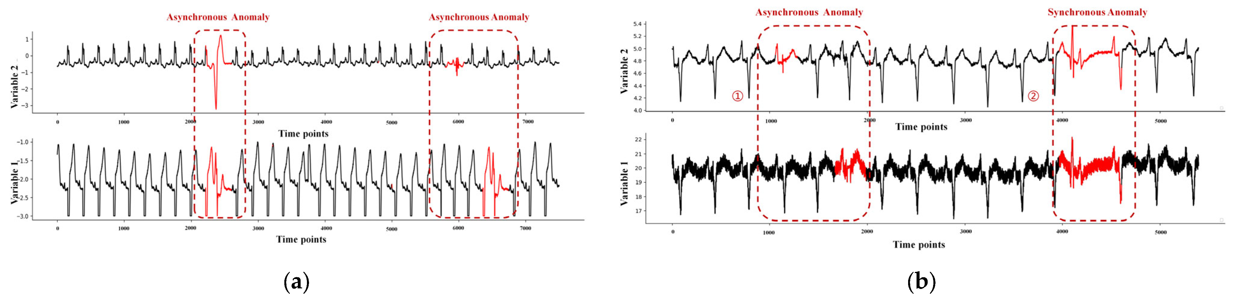
2.1. Anomaly Types for Multidimensional Time Series
2.1.1. Asynchronous Anomalies
2.1.2. Synchronous Anomalies
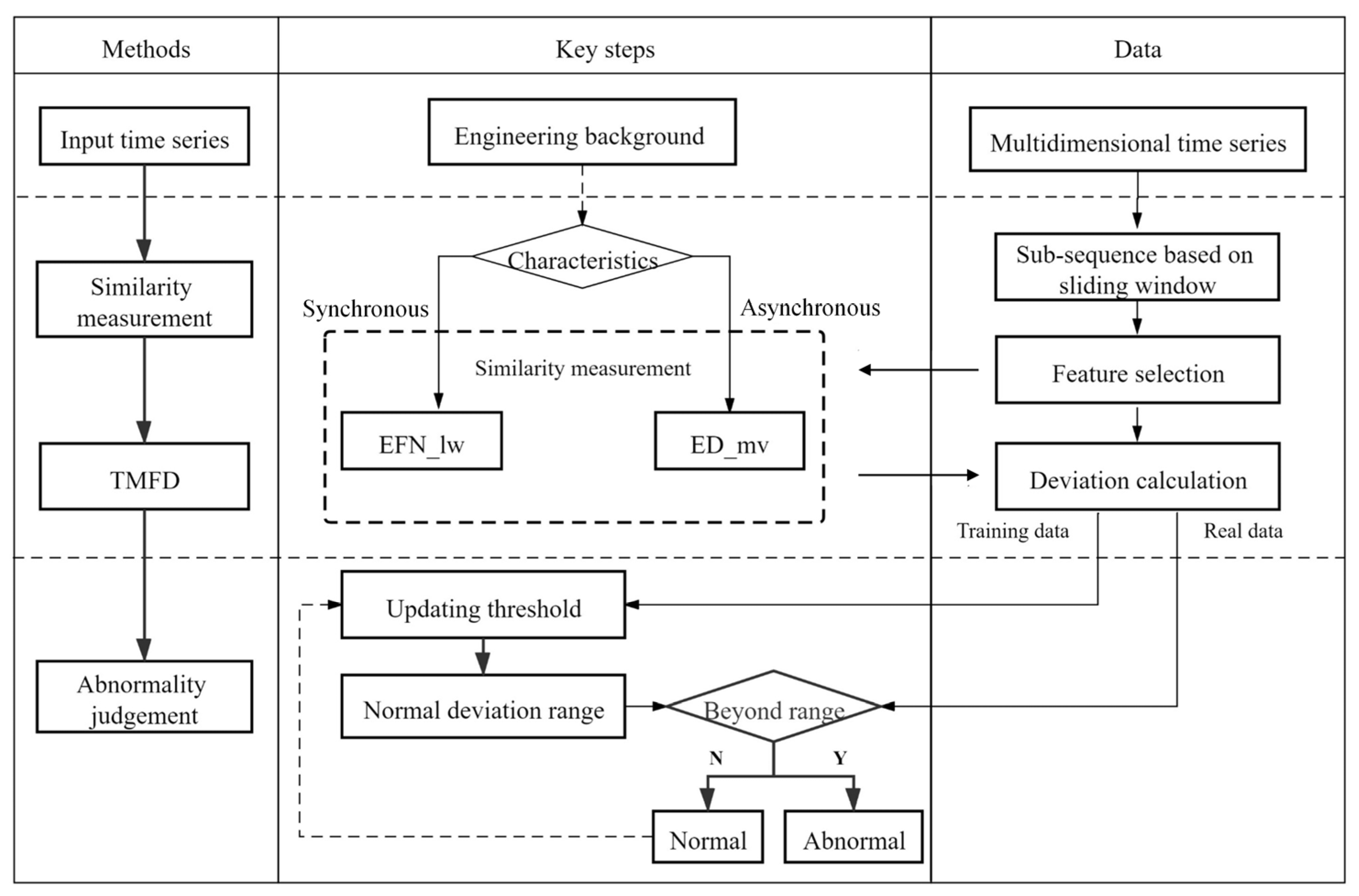
2.2. Algorithm Design
2.2.1. Detection Process
2.2.2. Matching Principle of Anomaly Types and Similarity Measurements
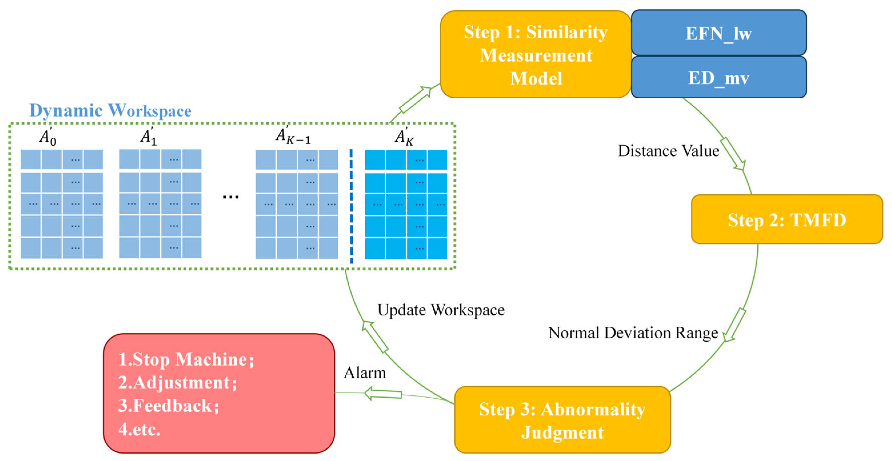
3. Algorithm Implementation
3.1. Overview
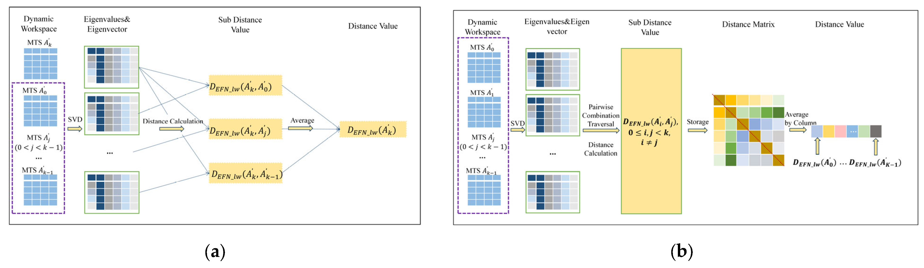
3.2. Similarity Measurement
3.2.1. EFN_lw
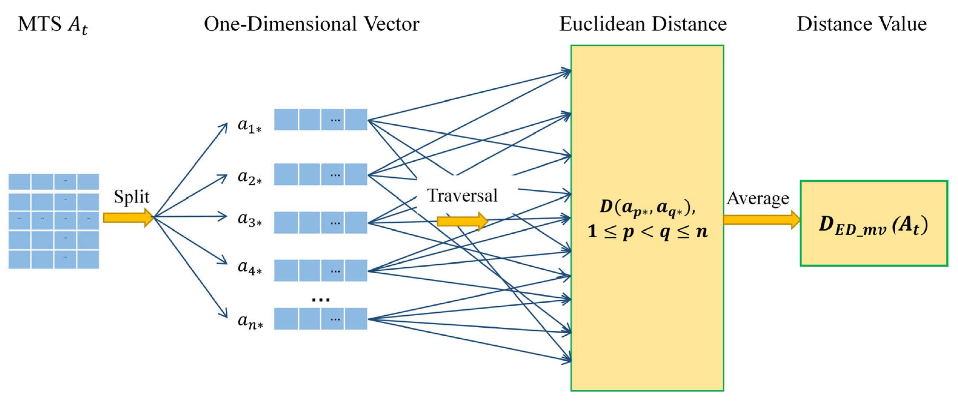
3.2.2. ED_mv
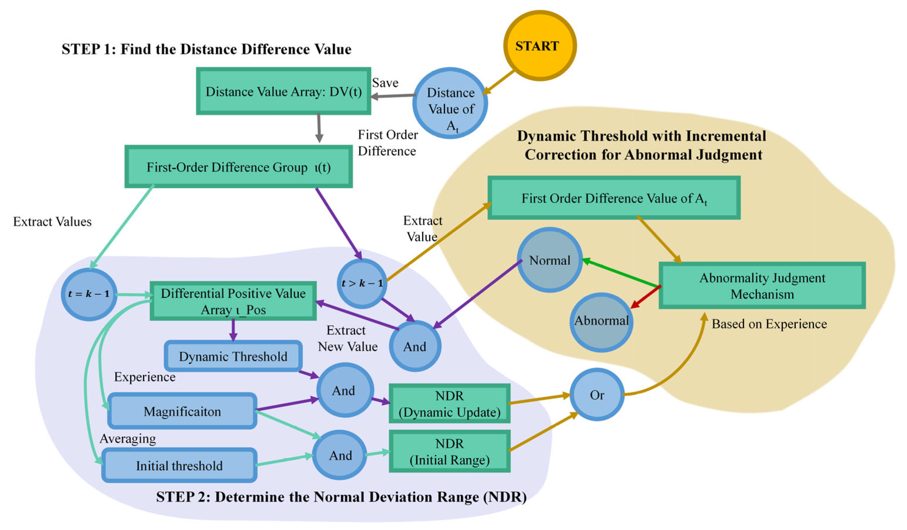
3.3. Threshold Mechanism Based on the First-Order Difference (TMFD)
3.4. Abnormal Judgement
4. Experiment Design and Analysis
4.1. Experiment Design
4.1.1. Data Sets
4.1.2. Experiment Procedure
4.1.3. Model Evaluation
4.2. Benchmark Data Set Experiments
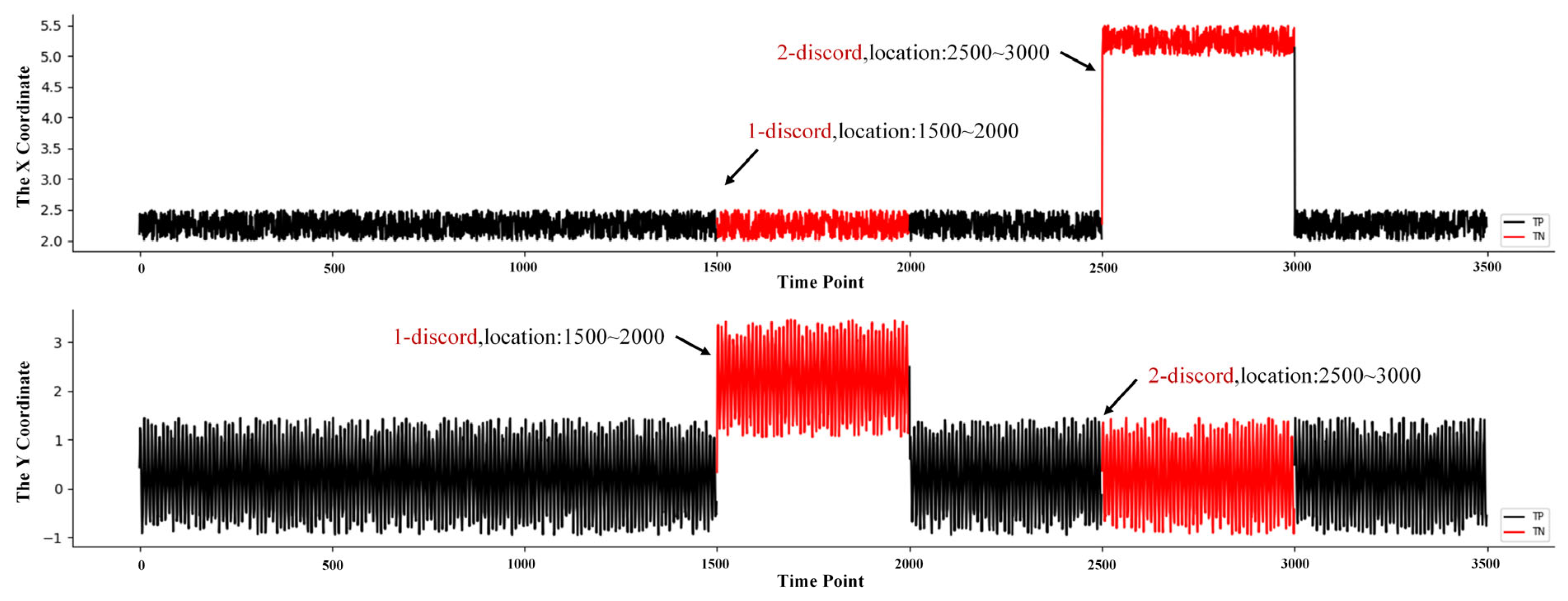
4.2.1. Manual Data Set
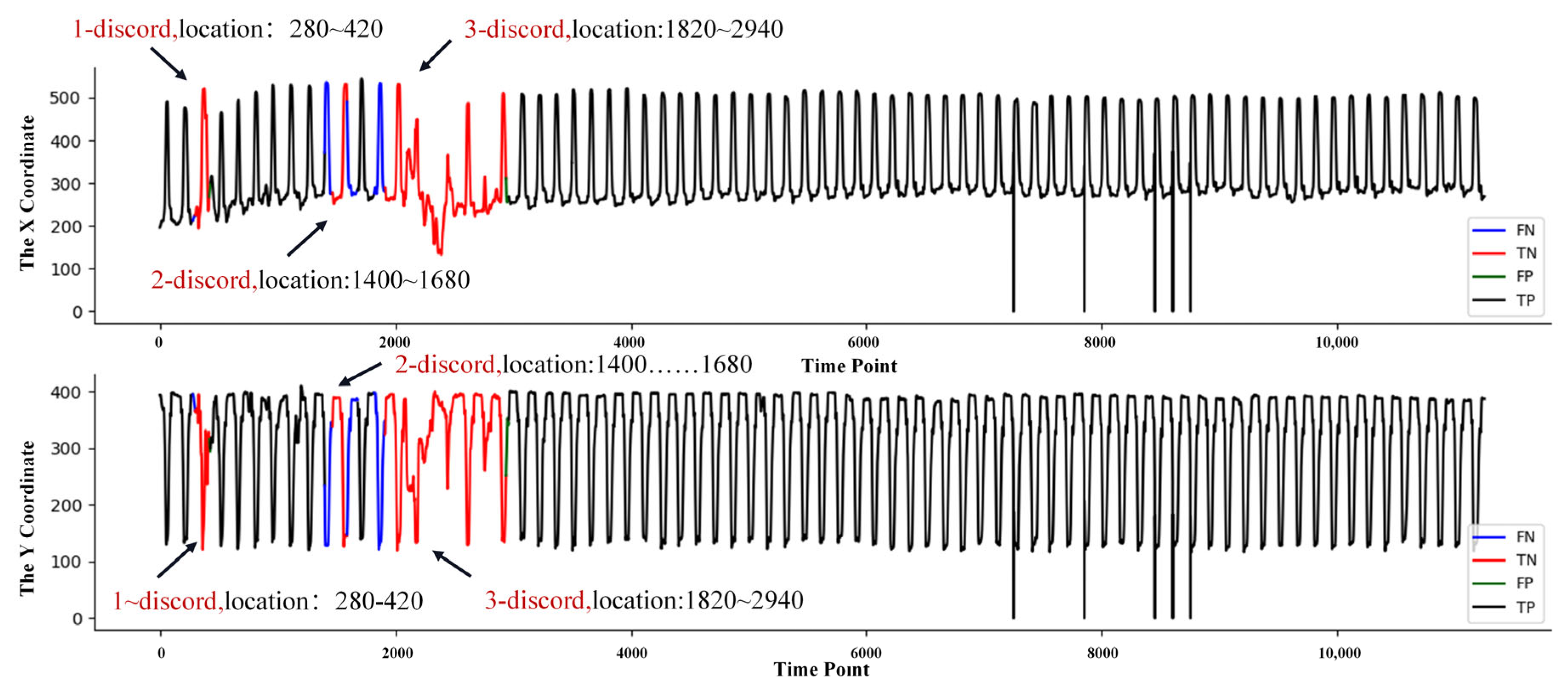
4.2.2. Video Surveillance Data Set
4.3. Engineering Validation
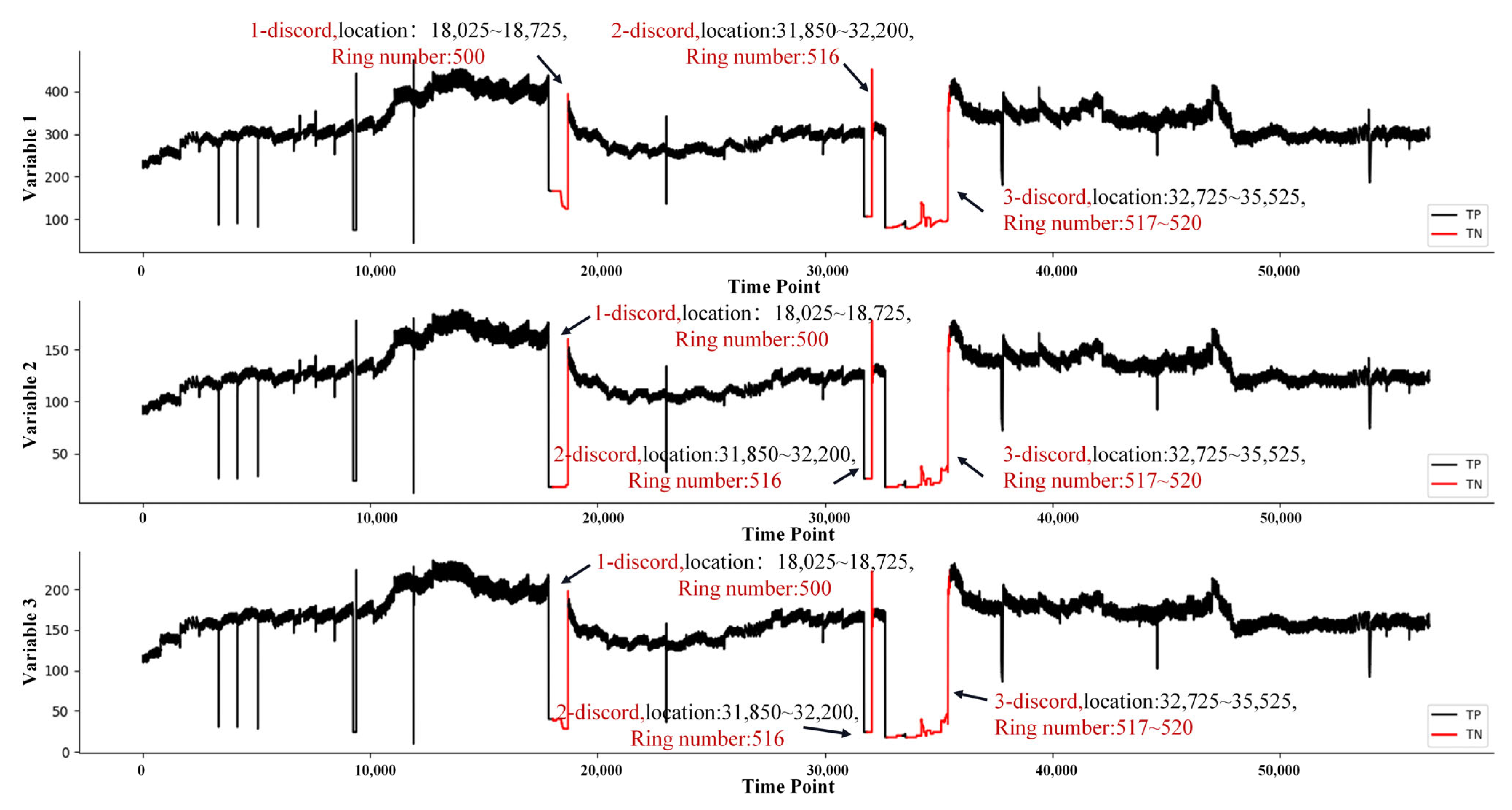
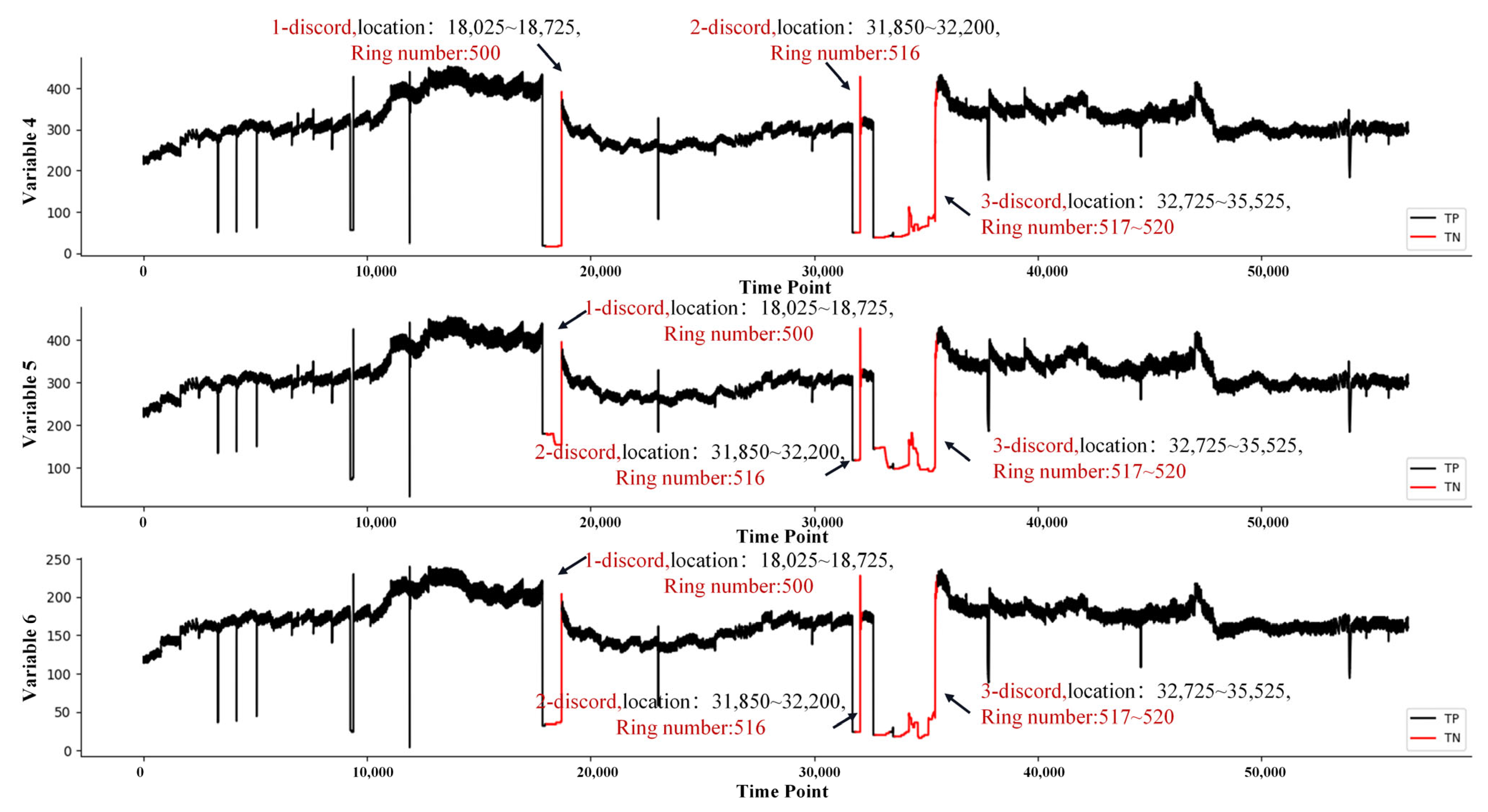
4.3.1. Grease System Data Set
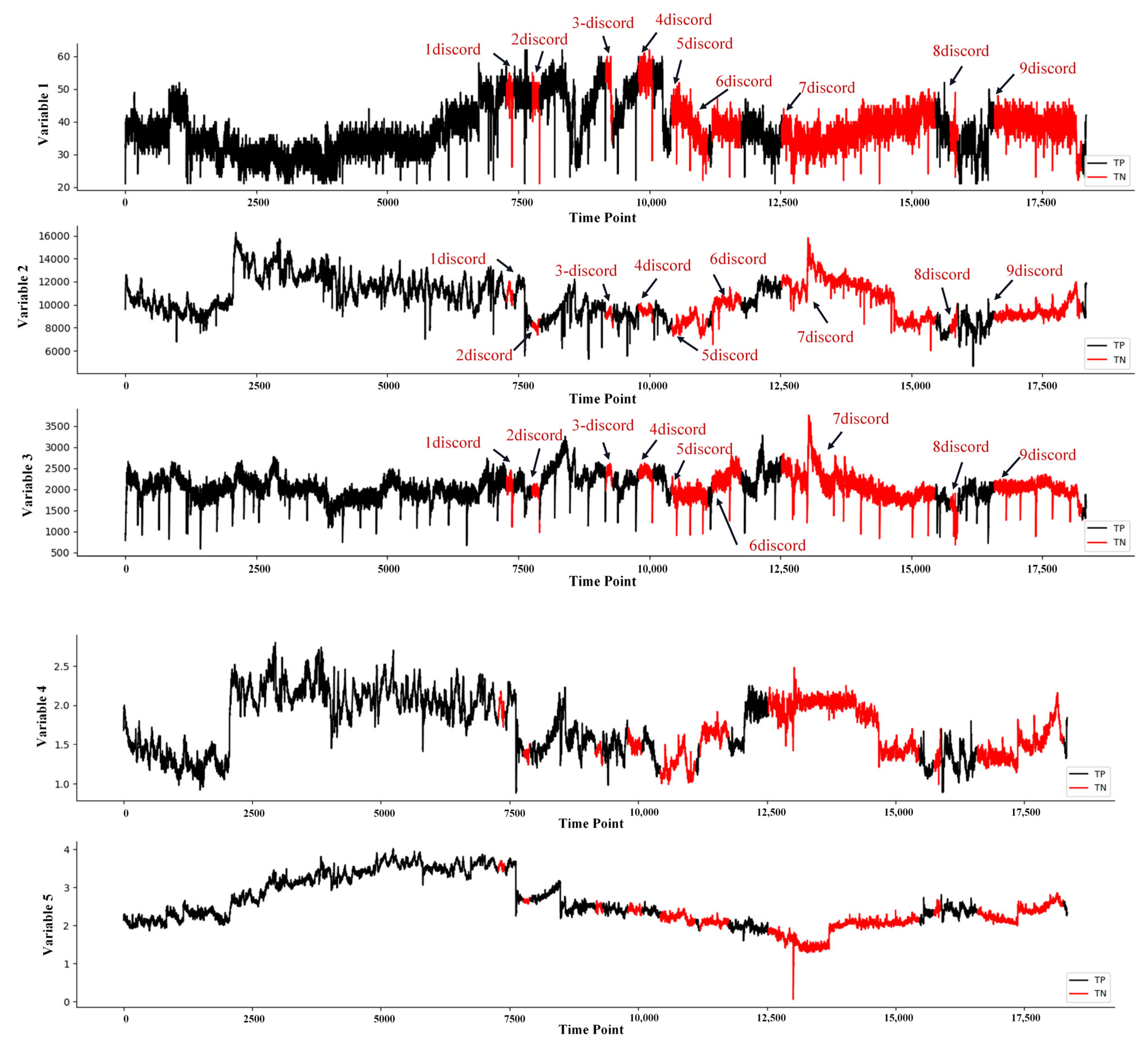
4.3.2. Propulsion System Data Set
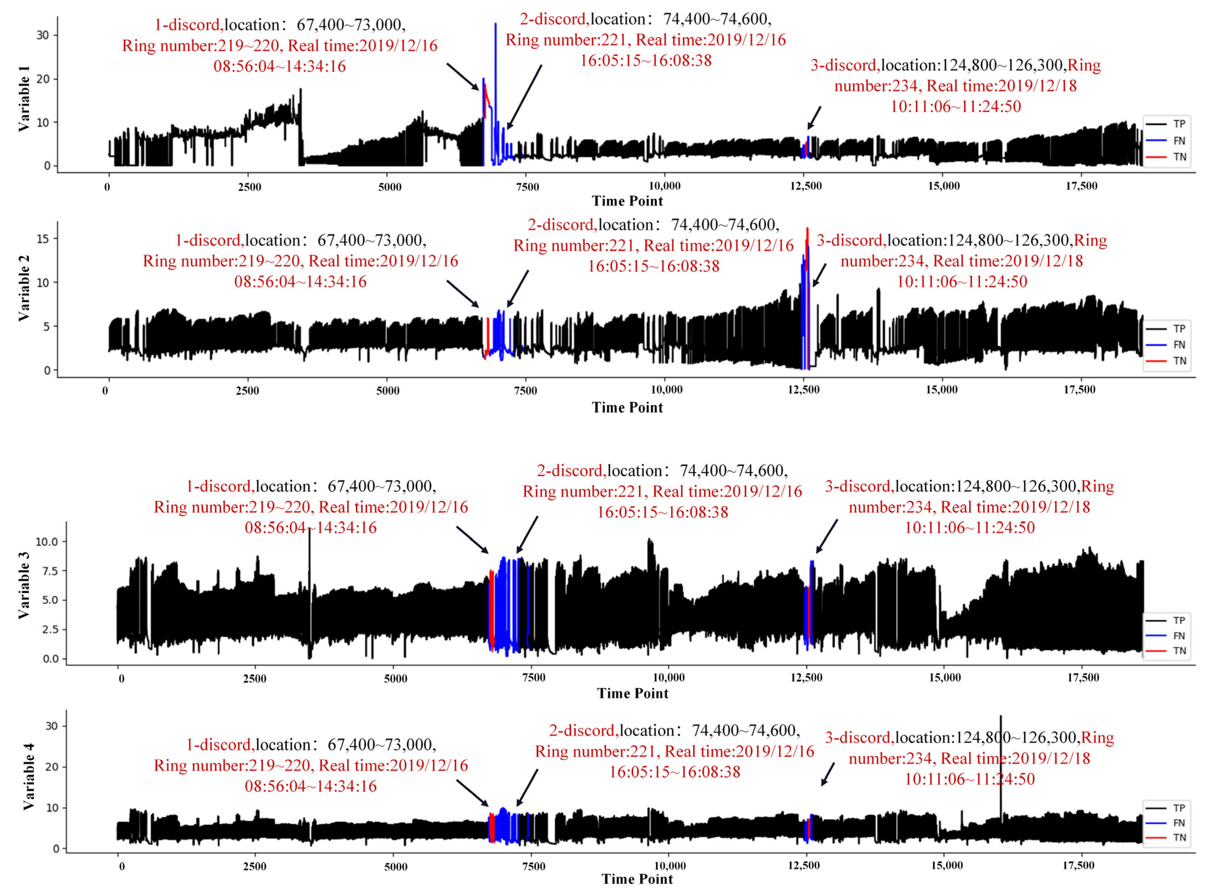
4.3.3. Grouting System Data Set
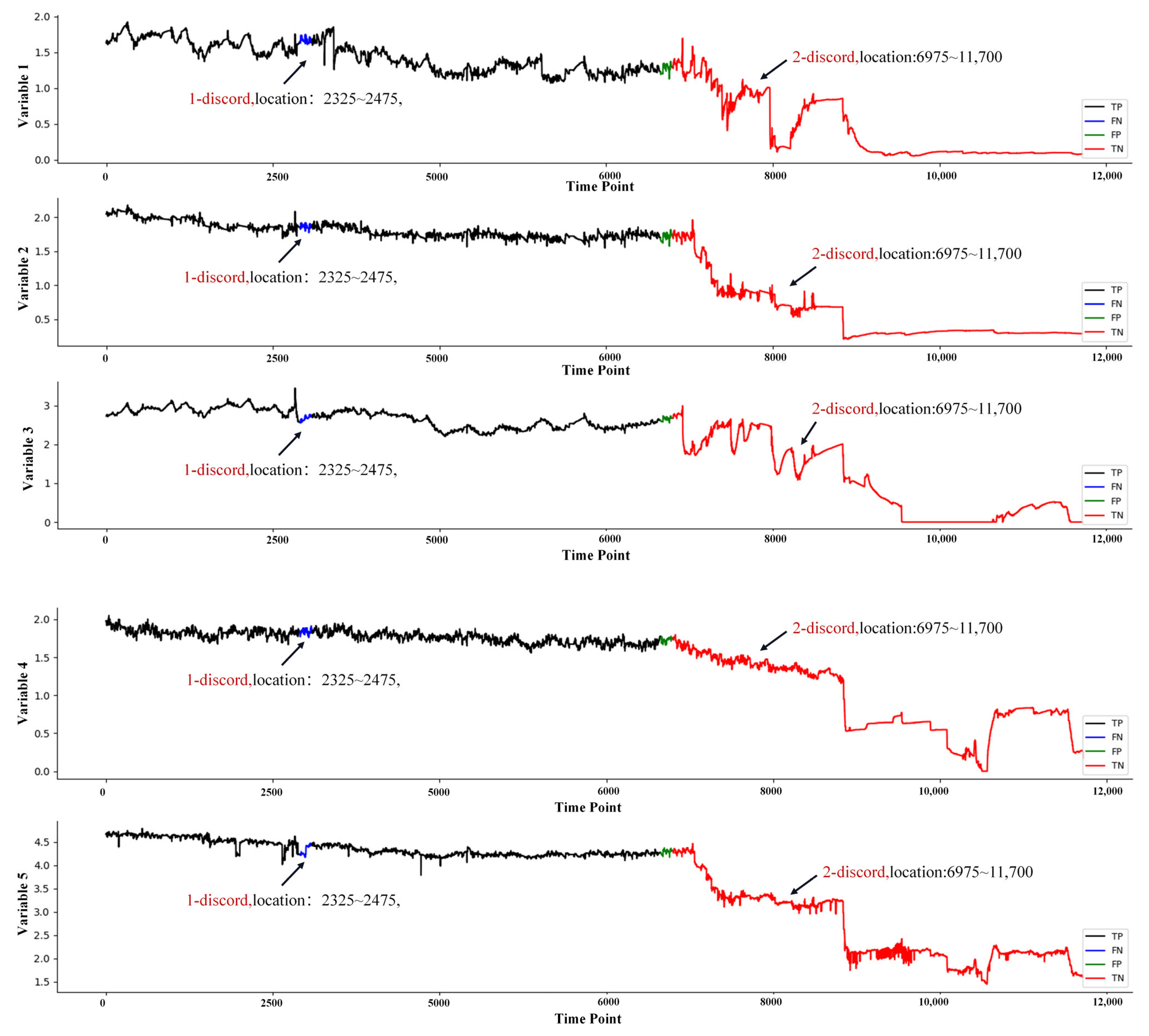
4.3.4. Pressure System Data Set
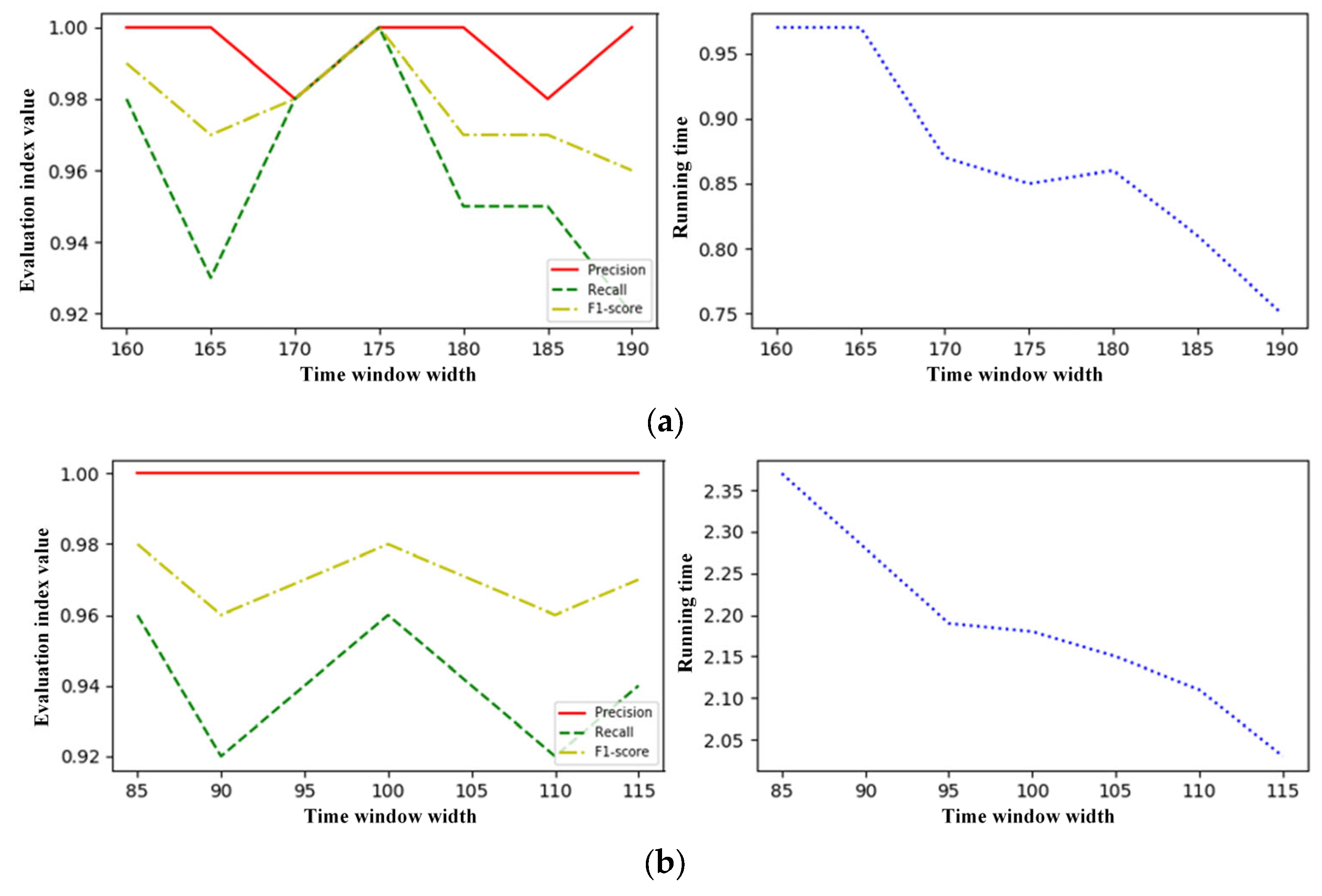
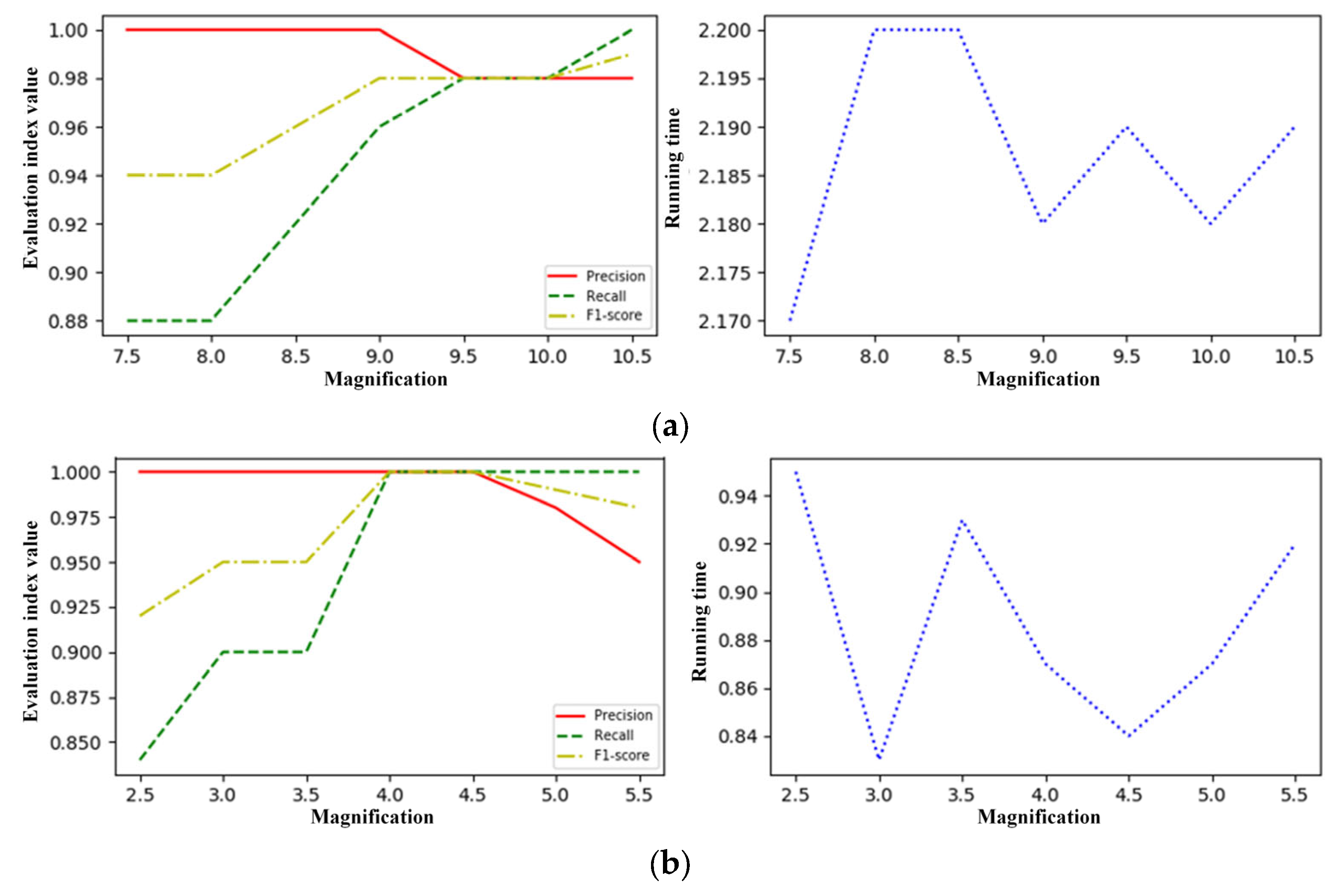
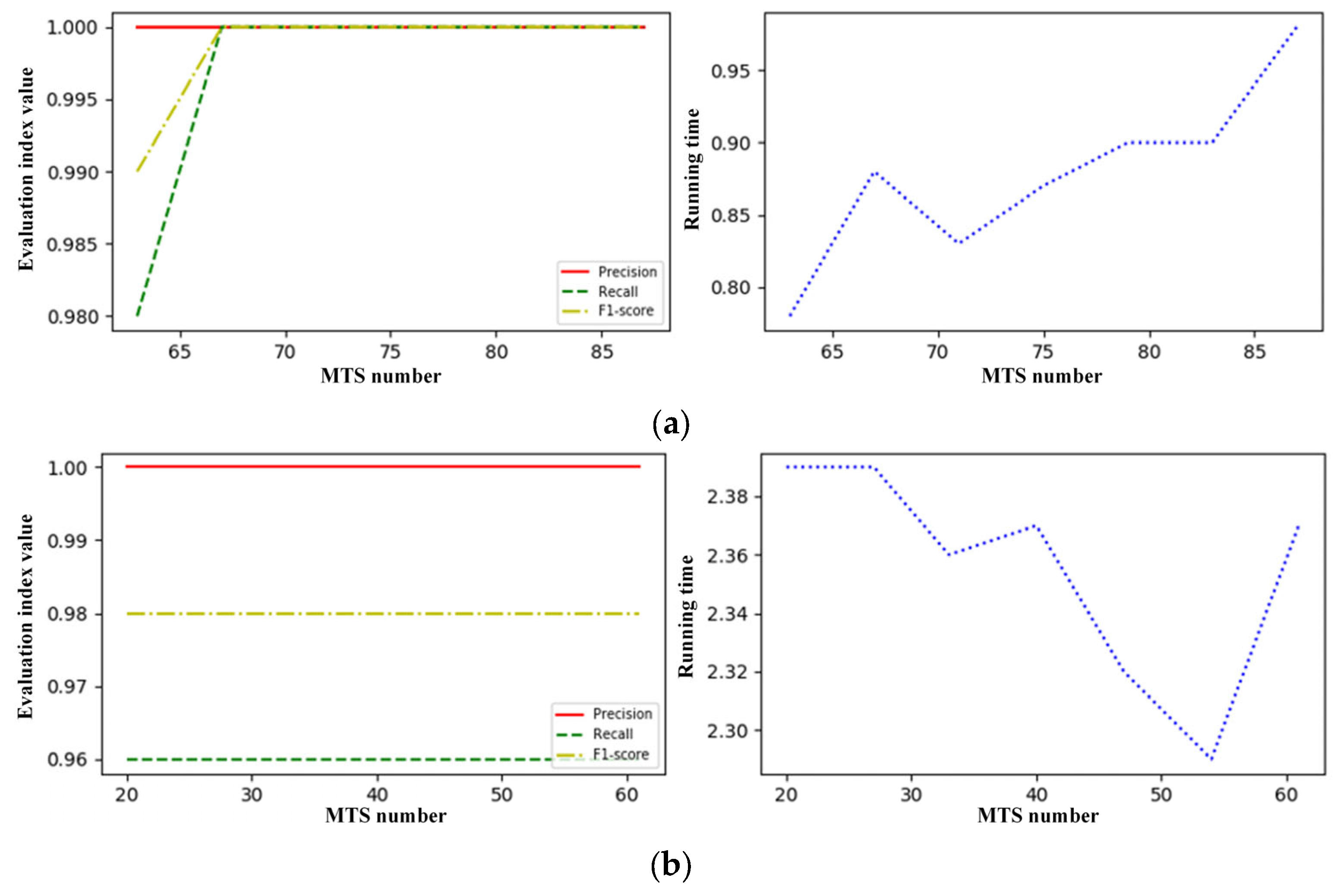
4.4. Parameter Sensitivity
4.5. Algorithm Performance
5. Conclusions
Author Contributions
Funding
Institutional Review Board Statement
Informed Consent Statement
Data Availability Statement
Conflicts of Interest
References
- Xiang, Y.; Tang, T.; Su, T.; Brach, C.; Liu, L.; Mao, S.S.; Geimer, M. Fast crdnn: Towards on site training of mobile construction machines. IEEE Access 2021, 9, 124253–124267. [Google Scholar] [CrossRef]
- Hu, M.; Bai, X.; Xu, W.; Wu, B. Review of anomaly detection algorithms for multi-dimensional time series. J. Comput. Appl. 2020, 40, 1553–1564. [Google Scholar] [CrossRef]
- Zhong, R.Y.; Xu, X.; Klotz, E.; Newman, S.T. Intelligent Manufacturing in the Context of Industry 4.0: A Review. Engineering 2017, 3, 616–630. [Google Scholar] [CrossRef]
- Habeeb, R.A.A.; Nasaruddin, F.; Gani, A.; Hashem, I.; Ahmed, E.; Imran, M. Real-time big data processing for anomaly detection: A Survey. IJIM 2018, 45, 289–307. [Google Scholar] [CrossRef]
- Ding, N.; Ma, H.; Gao, H.; Ma, Y.; Tan, G. Real-time anomaly detection based on long short-Term memory and Gaussian Mixture Model. Comput. Electr. Eng. 2019, 79, 106458. [Google Scholar] [CrossRef]
- Zhang, C.; Chen, Y.; Yin, A.; Qin, Z.; Zhang, X.; Zhang, K.; Jiang, Z.L. An Improvement of PAA on Trend-Based Approximation for Time Series. In Proceedings of the 18th ICA3PP 2018, Guangzhou, China, 15–17 November 2018; pp. 248–262. [Google Scholar]
- Hu, M.; Ji, Z.; Yan, K.; Guo, Y.; Feng, X.; Gong, J.; Zhao, X.; Dong, L. Detecting Anomalies in Time Series Data via a Meta-Feature Based Approach. IEEE Access 2018, 6, 27760–27776. [Google Scholar] [CrossRef]
- Navi, M.; Meskin, N.; Davoodi, M. Sensor fault detection and isolation of an industrial gas turbine using partial adaptive KPCA. J. Process Control 2018, 64, 37–48. [Google Scholar] [CrossRef]
- Roweis, S.T.; Saul, L.K. Nonlinear dimensionality reduction by locally linear embedding. Science 2000, 290, 2323–2326. [Google Scholar] [CrossRef] [PubMed]
- Canizo, M.; Triguero, I.; Conde, A.; Onieva, E. Multi-head CNN–RNN for multitime series anomaly detection: An industrial case study. Neurocomputing 2019, 363, 246–260. [Google Scholar] [CrossRef]
- Han, Z.J. An adaptive K-means initialization method based on data density. Comput. Appl. Softw. 2014, 31, 182–187. [Google Scholar]
- Kaur, R.; Kang, S.S. An enhancement in classifier support vector machine to improve plant disease detection. In Proceedings of the 2015 IEEE 3rd International Conference on MOOCs, Innovation and Technology in Education (MITE), Amritsar, India, 1–2 October 2015; pp. 135–140. [Google Scholar]
- Tran, K.P.; Nguyen, H.D.; Thomassey, S. Anomaly detection using Long Short Term Memory Networks and its applications in Supply Chain Management. IFAC-PapersOnLine 2019, 52, 2408–2412. [Google Scholar] [CrossRef]
- Wang, W.; Bao, J.; Li, T. Bound smoothing based time series anomaly detection using multiple similarity measures. J. Intell. Manuf. 2021, 32, 1711–1727. [Google Scholar] [CrossRef]
- Zheng, J.; Qu, H.; Li, Z.; Li, L.; Tang, X. A deep hypersphere approach to high-dimensional anomaly detection. Appl. Soft Comput. 2022, 125, 109146. [Google Scholar] [CrossRef]
- Li, J.; Izakian, H.; Pedrycz, W.; Jamal, I. Clustering-based anomaly detection in multivariate time series data. Appl. Soft Comput. 2021, 100, 106919. [Google Scholar] [CrossRef]
- Wang, X.; Pi, D.; Zhang, X.; Liu, H.; Guo, C. Variational transformer-based anomaly detection approach for multivariate time series. Measurement 2022, 191, 110791. [Google Scholar] [CrossRef]
- Wambura, S.; Huang, J.; Li, H. Robust Anomaly Detection in Feature-Evolving Time Series. Comput. J. 2021, 65, 1242–1256. [Google Scholar] [CrossRef]
- Audibert, J.; Michiardi, P.; Guyard, F.; Marti, S.; Zuluaga, M.A. Do Deep Neural Networks Contribute to Multivariate Time Series Anomaly Detection? Pattern Recognit. 2022, 132, 108945. [Google Scholar] [CrossRef]
- Gauci, M.; Chen, J.; Li, W.; Dodd, T.J.; Groß, R. Self-organized aggregation without computation. Int. J. Robot. Res. 2014, 33, 1145–1161. [Google Scholar] [CrossRef]
- Hawkins, D.M. A single outlier in normal samples. In Identification of Outliers, 3rd ed.; Springer: Dordrecht, The Netherlands, 1980; pp. 27–41. Available online: https://www.springer.com/cn/book/9789401539968 (accessed on 6 April 2024).
- Chandola, V.; Banerjee, A.; Kumar, V. Anomaly detection: A survey. ACM Comput. Surv. 2009, 41, 15. [Google Scholar] [CrossRef]
- Yang, K.; Shahabi, C. A PCA-based similarity measure for multivariate time series. In Proceedings of the 2nd ACM International Workshop on Multimedia Databases, Washington, DC, USA, 8–13 November 2004. [Google Scholar] [CrossRef]
- Guo, X.F.; Li, F. Analysis on similarity of multivariate time series based on Eros. Comput. Eng. Appl. 2014, 48, 111–114. [Google Scholar]
- Weng, X.Q.; Shen, J.Y. Outlier Mining for Multivariate Time Series Based on Sliding Window. Comput. Eng. 2007, 33, 102–104. [Google Scholar]
- Chen, Z. Research on Anomaly Detection and Data Quality Assessment of Bridge Health Monitoring Data. Master′s Thesis, Department of Engineering, Chongqing University, Chongqing, China, 2017. [Google Scholar]
- Wang, T.; Lu, G.; Yan, P. Multi-sensors based condition monitoring of rotary machines: An approach of multi-dimensional time-series analysis. Measurement 2019, 134, 326–335. [Google Scholar] [CrossRef]
- Kaya, H.; Gündüz-Öğüdücü, Ş. A distance based time series classification framework. Inf. Syst. 2015, 51, 27–42. [Google Scholar] [CrossRef]
- Keogh, E.; Lin, J.; Fu, A. HOT SAX: Efficiently finding the most unusual time series subsequence. In Proceedings of the Fifth IEEE International Conference on Data Mining (ICDM′05), Houston, TX, USA, 27–30 November 2005. [Google Scholar] [CrossRef]
- Hu, M.; Wu, F.F.; Zhu, B.; Lu, B.; Pu, J.L. A New Hazard Identification Method-State Transition Graph. Appl. Mech. Mater. 2011, 48–49, 71–78. [Google Scholar] [CrossRef]
- Malhotra, P.; Vig, L.; Shroff, G.; Agarwal, P. Long Short Term Memory Networks for Anomaly Detection in Time Series. Presented at ESANN. [Online]. Available online: http://www.i6doc.com/en/ (accessed on 6 April 2024).


| Similarity Measure Methods | Selection Criteria | Anomaly Type | |
|---|---|---|---|
| MTS Correlation | Temporal Attributes of MTS Abnormal Events | ||
| ED_mv | Strong | Consistency | Synchronous anomaly |
| EFN_lw | Strong | Inconsistency | Asynchronous anomaly |
| Weak | Consistency or Inconsistency | ||
| No | Data Set Name | Dimensionality | Total Sample Size | Training Sample Size | Real Discord | Data Sources |
|---|---|---|---|---|---|---|
| 1 | Manual | 2 | 3500 | 1000 | 1500–2000, 2500–3000 | Composite data |
| 2 | Video Surveillance | 2 | 11,250 | 1400 | 300–430, 1465–1590, 1913–2964 | [28,29] |
| 3 | Grease System | 6 | 56,580 | 13,125 | 500, 516–520 (RingNo) | Shanghai Metro Line 13 |
| 4 | Propulsion System | 5 | 18,340 | 3500 | 947–959 (RingNo) | Hangzhou Wenyi Tunnel Project |
| 5 | Grouting System | 4 | 186,320 | 4000 | 2019/12/16 09:02–15 (RingNo:219) 2019/12/18 11:11:15 (RingNo:234) | Hangzhou Shaoxing Metro Project |
| 6 | Pressure System | 5 | 11,720 | 2250 | 6650–11,720 | Tunnel Project in Shanghai [30] |
| Number | Data Set Name | Time Window Length | Magnification | MTS Number in Workspace |
|---|---|---|---|---|
| 1 | Grease System | 175 | 4 | 75 |
| 2 | Propulsion System | 70 | 3 | 50 |
| 3 | Grouting System | 100 | 9 | 40 |
| 4 | Pressure System | 75 | 4 | 30 |
| Method | Time of Grouting System Data Set (s) | Time of Pressure System Data Set (s) |
|---|---|---|
| EFN_lw | 0.5939 | 0.3047 |
| Eros | 0.8753 | 0.4581 |
Disclaimer/Publisher’s Note: The statements, opinions and data contained in all publications are solely those of the individual author(s) and contributor(s) and not of MDPI and/or the editor(s). MDPI and/or the editor(s) disclaim responsibility for any injury to people or property resulting from any ideas, methods, instructions or products referred to in the content. |
© 2024 by the authors. Licensee MDPI, Basel, Switzerland. This article is an open access article distributed under the terms and conditions of the Creative Commons Attribution (CC BY) license (https://creativecommons.org/licenses/by/4.0/).
Share and Cite
Wu, B.; Zhang, F.; Wang, Y.; Hu, M.; Bai, X. Anomaly Detection Algorithm for Urban Infrastructure Construction Equipment based on Multidimensional Time Series. Sustainability 2024, 16, 3335. https://doi.org/10.3390/su16083335
Wu B, Zhang F, Wang Y, Hu M, Bai X. Anomaly Detection Algorithm for Urban Infrastructure Construction Equipment based on Multidimensional Time Series. Sustainability. 2024; 16(8):3335. https://doi.org/10.3390/su16083335
Chicago/Turabian StyleWu, Bingjian, Fan Zhang, Yi Wang, Min Hu, and Xue Bai. 2024. "Anomaly Detection Algorithm for Urban Infrastructure Construction Equipment based on Multidimensional Time Series" Sustainability 16, no. 8: 3335. https://doi.org/10.3390/su16083335
APA StyleWu, B., Zhang, F., Wang, Y., Hu, M., & Bai, X. (2024). Anomaly Detection Algorithm for Urban Infrastructure Construction Equipment based on Multidimensional Time Series. Sustainability, 16(8), 3335. https://doi.org/10.3390/su16083335