Abstract
We propose a method to identify the congestion driver sources contributing to the major traffic congestion of a regional (Hunan province) freeway network. The results indicate that the congestion driver sources are mostly observed during heavy traffic periods and mainly distributed in the regions surrounding Changsha (the capital of Hunan province) and the regions adjacent to other provinces and freeway interconnecting hubs. Moreover, we develop a method to analyze the major driver sources of a local freeway section. Using the method, the trips affected by traffic accidents or road maintenance works can be identified well. Our findings and the proposed methods could facilitate the deployment of effective traffic control countermeasures and the development of sustainable regional transportation.
1. Introduction
Freeways are characterized by good features of high speed and large capacity [1,2]. Many countries in the world have built well-connected freeway networks [3]. Over the past 10 years, the freeway transportation infrastructure of China has experienced rapid development, with the total length of freeway increases from 96,200 km in 2012 to nearly 180,000 km in 2022 [4,5]. Given its fast speed, wide coverage, and good connection, the freeway has become a more favorable transportation mode for many travelers [6]. Taking Hunan (i.e., a southern province of China) freeway as an example, the annual average daily traffic volume has increased from 25,725 in 2017 to 29,283 in 2022 [7,8]. The rapidly growing travel demand [9] poses great pressure to freeway infrastructures, which inevitably causes frequent, and sometimes severe, traffic congestions. Traffic congestion not only downgrades the freeways’ level of service [10] but also increases the accidental risks [11], posing a great challenge to the development of sustainable freeway transportation.
The effective implementation of various freeway traffic control approaches (e.g., on-ramp control, variable speed limit, route guidance) [12,13,14] relies on an in-depth understanding of the traffic congestion pattern in freeways [15]. To this end, many researchers have investigated freeway traffic congestion patterns. Chen et al. [16] used floating car data to uncover the spatiotemporal distribution of traffic congestion in the east fourth ring of the Beijing urban freeway. Yang et al. [17] found that traffic congestion was more likely to occur at the segments connecting the main roads, the segments located upstream of on-ramps or off-ramps, and the segments with oversaturated traffic volumes. Sarvi et al. [18] studied the patterns of traffic congestion in the Tokyo freeway. Fernando [19] analyzed the location and duration of traffic congestion caused by mass events. Pei et al. [20] employed density clustering algorithms to analyze the spatiotemporal distribution of traffic congestion in cold weather. Ren et al. [21] identified the congested segments when there were traffic accidents. Ghosh et al. [22] employed a delay time index to analyze the traffic congestion patterns when a road was under construction. In addition, traffic congestion can be detected by predicting the travel demand [23,24,25].
Despite the extensive investigations into traffic congestion patterns, we are still lacking a comprehensive understanding of which vehicles or drivers contribute to major traffic congestion in freeways. In the freeway transportation context, driver sources include the toll stations which a large number of vehicles pass through, creating congested freeway sections [26,27]. Moreover, researchers have developed on-ramp control methods and route guidance methods based on driver source information [27,28,29], finding that driver source information can improve the congestion mitigation effect and reduce the difficulty of implementing traffic control schemes [27,28,29]. Yet, the spatiotemporal patterns of freeway driver sources, which are crucial for deploying effective traffic control countermeasures and developing sustainable regional transportation systems, are still not well understood.
In this study, we use the travel demand data of Hunan freeway to identify the network-wide congestion driver sources and the local section major driver sources. Firstly, we identify the congestion driver sources (CDSs) which contribute to major traffic congestion in the Hunan freeway network and analyze their spatiotemporal patterns. Secondly, we analyze the major driver sources (MDSs) of local freeway sections. The trips affected by traffic accidents or road maintenance works can be effectively identified. The discovered spatiotemporal patterns of CDSs and MDSs can be used to assist freeway congestion mitigation and freeway emergency responses.
The remainder of this paper is organized as follows. Section 2 introduces the data used in the present study. Section 3 introduces the methods for assigning the travel demand and identifying the driver sources. Section 4 analyzes the spatiotemporal patterns of congestion driver sources in the Hunan freeway network. Section 5 analyzes the major driver sources of two local freeway sections affected by a traffic accident and road maintenance work. Section 6 discusses the correlation between the number of driver sources and the travel demand and explores whether the spatial distribution of CDSs is related to their topological importance. Section 7 concludes the research findings and discusses future research directions.
2. Data
2.1. Geographic Information Data of the Freeway Network
The Hunan freeway network data were provided by the Hunan Communications Research Institute Co., Ltd. (Changsha, China) and the Baidu Map Open Platform (Beijing, China). The data included the freeway ID, the freeway section ID, the origin toll station ID, and the destination toll station ID of each freeway section. The data also included the coordinates of each toll station and the length of each freeway section. The speed limit information and information on the number of lanes of each freeway section were collected from Baidu Map and the official website of the China freeway (https://www.chinahighway.com/ (accessed on 28 February 2024)). The capacity of each freeway section was estimated according to the standard formulated by the Ministry of Transportation of the People’s Republic of China (Table 1). A total of 449 toll stations and 1100 freeway sections were recorded in the dataset. The spatial distribution of the toll stations is shown in Figure 1a, where the administrative zone of each county is also depicted. The Hunan freeway network is shown in Figure 1b.

Table 1.
The standards for estimating the capacity of a freeway section.
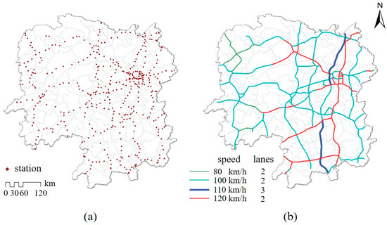
Figure 1.
The geographic information data of the Hunan freeway network. (a) The spatial distribution of freeway toll stations in Hunan province and (b) the Hunan freeway network. The color of a section indicates its speed limit, whereas the width of a section indicates the number of lanes.
2.2. Freeway Travel Demand Data
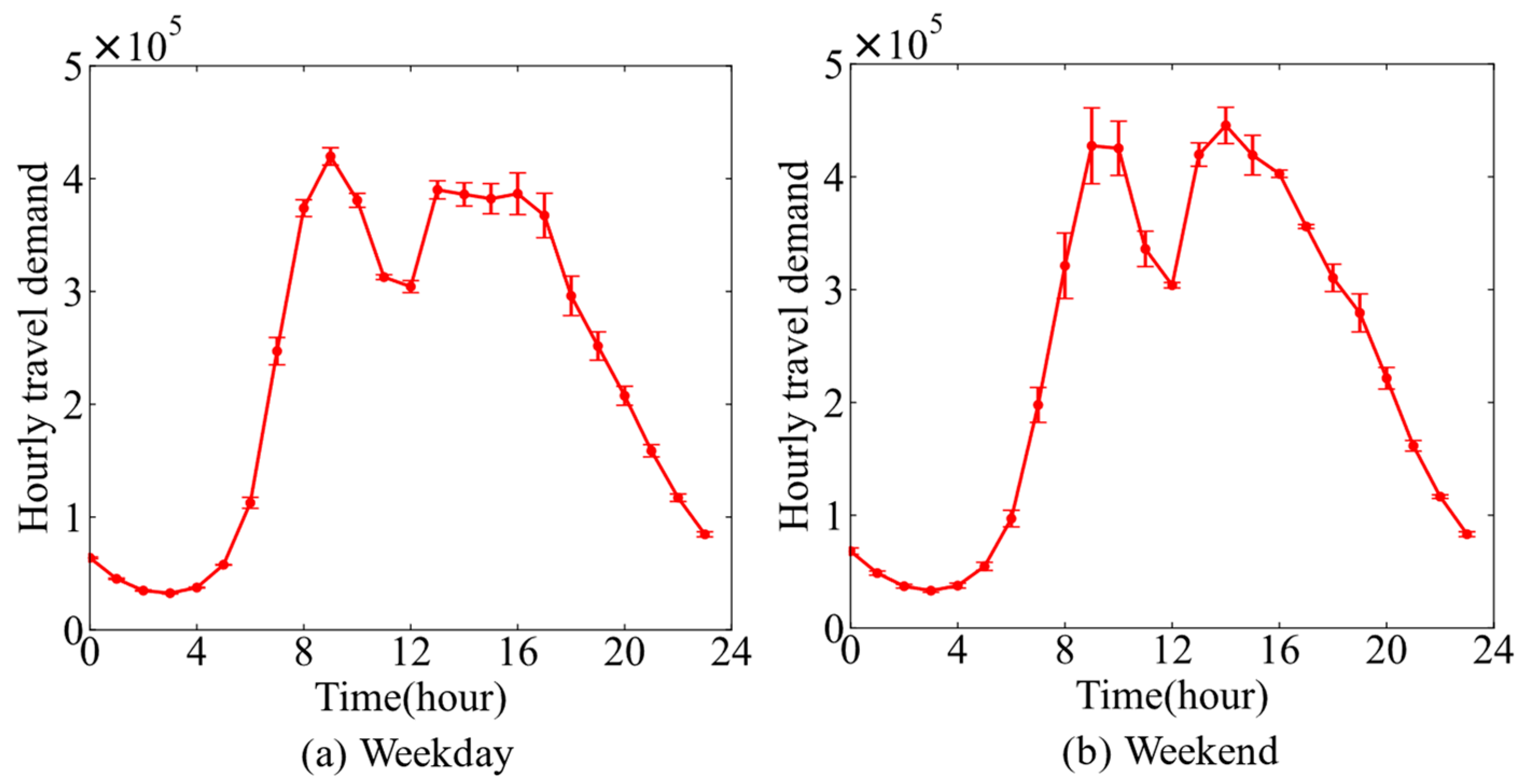
The Hunan freeway travel demand data were also provided by the Hunan Communications Research Institute Co., Ltd. The travel demand data included the number of trips between each pair of toll stations during each one-hour time window in March and April 2019. We mainly analyzed the data collected during an ordinary week from 11 March to 17 March (no events occurred, e.g., traffic accidents, festivals, epidemics, or extreme weather). We calculated the average number of freeway trips during each time window. As shown in Figure 2a, there was only one morning peak time window (9:00 a.m.–10:00 a.m.) on weekdays and the travel demand remained relatively large throughout the whole afternoon. However, on weekend days, there was a morning peak time window (9:00 a.m.–10:00 a.m.) and an afternoon peak time window (14:00 p.m.–15:00 p.m.). Interestingly, the freeway rush hours are different from those observed in urban transportation [30,31], highlighting the different mobility patterns of freeway travelers and city travelers.
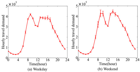
Figure 2.
The average number of freeway trips during each one-hour time window from 11 March 2019 to 17 March 2019. The error bars represent the standard deviations in the number of freeway trips during each one-hour time window.
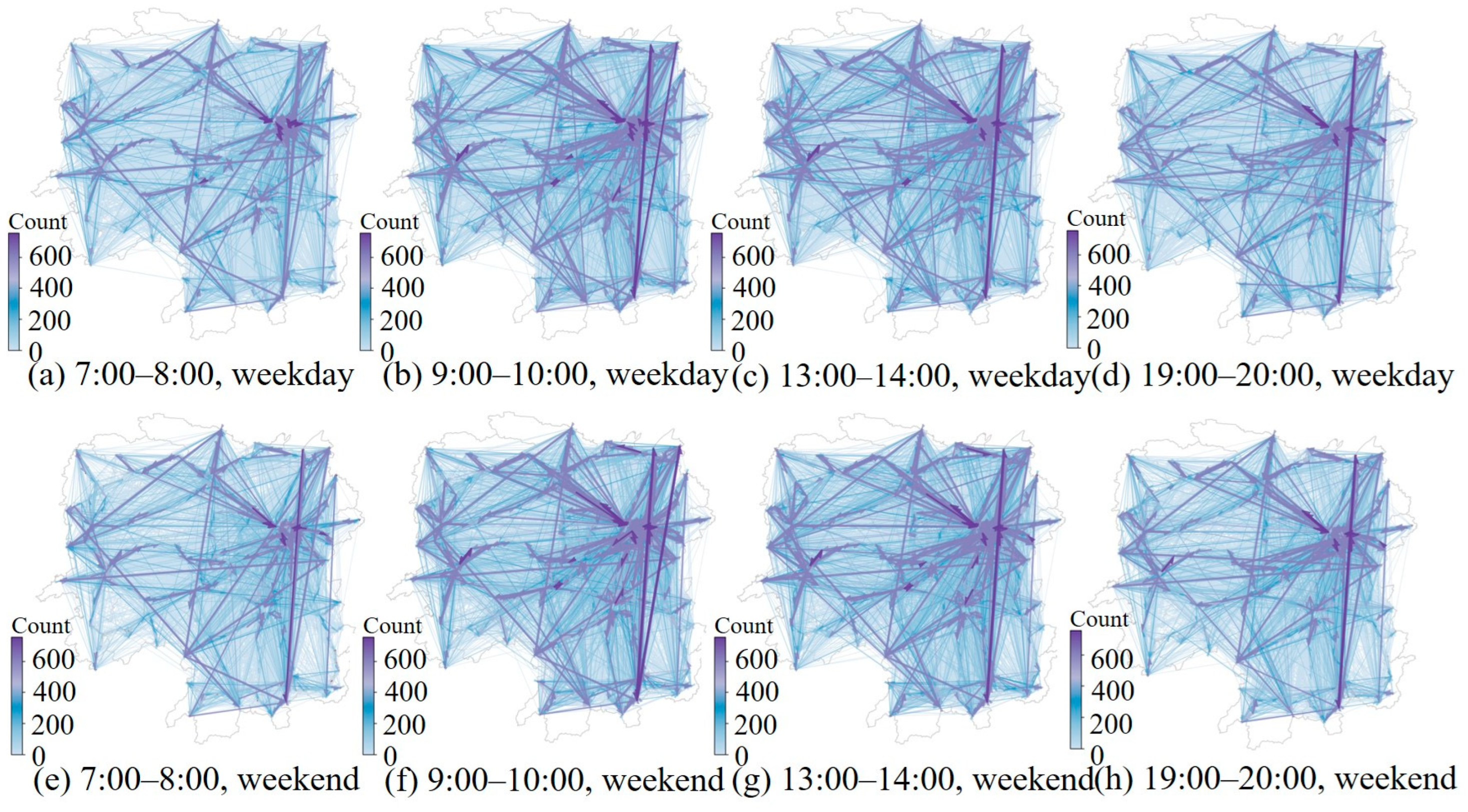
As shown in Figure 3, the spatial distribution of freeway travel demand is pretty stable across different time windows. Most origin–destination (O–D) pairs are featured with small travel demands. However, large travel demands are observed among a few toll stations located at the southern and northern border areas, which could be attributed to the long-distance trips occurring which pass through Hunan province. In addition, many O-D pairs with their origins or destinations located in Changsha are featured with large travel demands, which is not surprising because Changsha is the capital of Hunan province. Finally, a few O-D pairs around the cities of Changde, Huaihua, and Hengyang are also characterized by large traffic volumes, which could be caused by the strong attraction of cities to mobility flows.
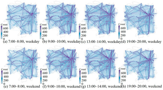
Figure 3.
The spatial distribution of freeway travel demands across different time windows. The color of each directed line illustrates the travel demand posed on the O-D pair.
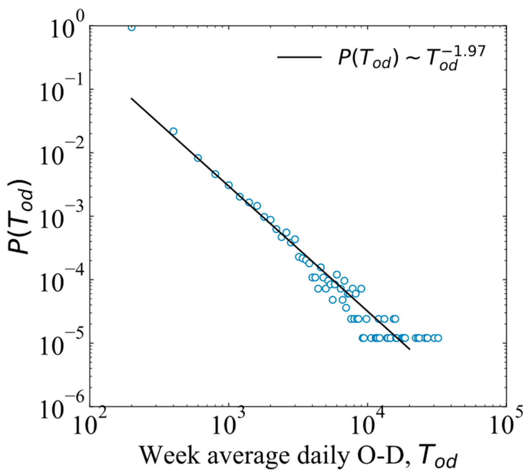
Heterogeneity indicates that the values of a quantity have a wide span and show significant differences. To analyze the heterogeneity of travel demand, we calculated a week’s average daily travel demand for each O-D pair. We found that can be well approximated by a power law distribution , implying that travel demands are heterogeneously distributed (Figure 4). The heterogeneously distributed travel demand determines the unevenly distributed traffic flow on the freeway network, suggesting that some freeway sections may suffer severe traffic congestion.
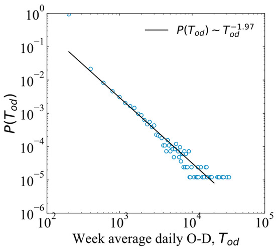
Figure 4.
The week’s average daily travel demands of O-D pairs follow a power law distribution.
3. Methodology
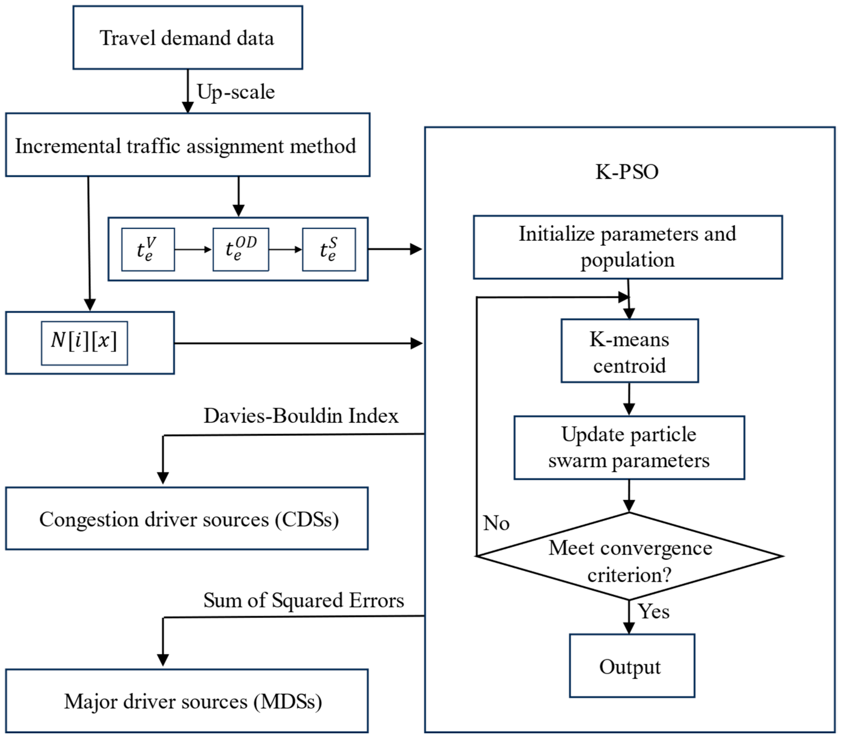
In this section, we introduce the method for assigning the travel demand to the freeway network, the method for estimating the extra travel times of vehicles, O-D pairs, and toll stations, and the method for identifying the congestion driver sources of the freeway network and the major driver sources of local freeway sections. Figure 5 illustrates the flowchart of the proposed methodology.
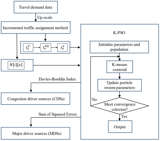
Figure 5.
Flowchart of the proposed methodology.
3.1. Inferring the Vehicle Path and Estimating the Traffic Flow
In this study, we employed the incremental traffic assignment (ITA) method to assign the travel demand to the freeway network. The ITA method was selected because it can approximate equilibrium traffic assignment and has a low computation cost [32]. When applying the ITA method, the O-D matrix was first split into four sub-OD matrices, which, respectively, contained 40%, 30%, 20%, and 10% of the trips randomly selected from the travel demand data. Next, the trips in the first sub-OD matrix were assigned to the freeway network using the Dijkstra algorithm [33]. The travel cost of each freeway section was updated using the BPR function (Equation (1)). This process continued until all trips in the sub-OD matrices had been assigned.
In Equation (1), is the capacity of a freeway section ; is the traffic flow of ; is the set of freeway sections; is the free-flow travel time of ; and the coefficients and are set to 0.5668 and 1.4331 according to practical measurements [34,35].
Volume over capacity was used to quantify the level of traffic congestion:
We further calculated the average daily of the Hunan freeway network in a week:
where is the weekly average traffic flow of freeway section ; is the length of ; and is the number of one-hour time windows within a day (i.e., 24). We used the travel demand data collected from 11 March to 17 March 2019 to calculate the week’s average daily , finding that the was only 0.055, which is much smaller than that reported by the Department of Transportation of Hunan province (i.e., 0.386). To solve this, we up-scaled the travel demand between each pair of toll stations by 7 times to simulate the actual traffic condition.
3.2. Identifying the Congestion Driver Sources of the Hunan Freeway Network
We defined the congestion driver sources of the freeway network by first calculating the total extra travel time of all vehicles entering the freeway from each toll station during each time window . Next, a threshold was determined for the total extra travel time using the K-PSO algorithm. The toll stations with a longer than the threshold were identified as the congestion driver sources (CDSs).
Firstly, the total extra travel time of a toll station was calculated based on the extra travel time of each vehicle and the total extra travel time of each O-D pair :
where and are the actual travel time and the free-flow travel time of a vehicle entering origin toll station during time window and exiting destination toll station , is the set of vehicles entering and exiting during , and is the set of destination toll stations of trips entering during .
Secondly, the threshold of was determined using the K-PSO algorithm, which combines the advantages of K-means clustering and Particle Swarm Optimization (PSO). We used the K-PSO algorithm to cluster the total extra travel times of toll stations. The upper limit of the cluster with the smallest was determined as the threshold of . More details of the K-PSO algorithm are elaborated upon as follows [36]:
Step 1: initialize the number of clusters , the learning factor , the inertia weight , and the number of particles in the particle swarm.
Step 2: Initialize the particle in the population. The particle position is defined as and the velocity of the particle is defined as , where represents the dimension of . Each element in and is randomly generated and ranges from 0 to 1. We used the K-means algorithm to split the extra travel times into clusters and calculate the centroid of each cluster. The fitness was evaluated using the sum of squared distances between and the cluster centroid. The particle swarm containing particles was generated:
Step 3: Calculate the individual optimal position of each particle and the optimal position of the population. for each particle and is equal to the position of the particle with the smallest fitness value.
Step 4: update the velocity and position of each particle using Equations (8) and (9).
where .
Step 5: Perform K-means clustering using the updated positions of particles and the current centroids. Reassign particles to the nearest cluster centroid based on their positions and calculate the fitness value.
Step 6: For each particle , the fitness value of its current position is compared with the fitness value of the particle’s historical optimal position . Set if . Similarly, for each particle , the fitness value of its optimal position is compared with the fitness value of the optimal position of the particle swarm. Set if .
Step 7: stop the algorithm when the maximum number of iterations is reached and output the clustering results; otherwise, repeat steps 4–6.
Step 8: Change the number of clusters and repeat steps 1–7. Use the Davies–Bouldin index to evaluate the effectiveness of clustering. The optimal K value is determined when the Davies–Bouldin index reaches the smallest value.
3.3. Identifying the Major Driver Sources of Local Freeway Sections
We analyzed the number of vehicles departing from each toll station (i.e., driver source) and passing a freeway section . Next, we calculated the proportion of traffic flow contributed by each driver source and ranked the driver sources in descending order according to . We defined the major driver sources (MDSs) of a local freeway section as the top-ranking sources that cumulatively contribute a certain portion (exceeding a threshold) of the section’s traffic flow. The threshold portion was determined using the K-PSO algorithm. Specifically, we used the K-PSO algorithm to cluster the proportion of traffic flow contributed by each driver source , and the upper limit of the cluster with the smallest was determined as the threshold proportion of traffic flow contribution . The driver sources contributing a portion of traffic flow were identified as the MDSs of the freeway section.
Using the Davies–Bouldin index would have generated too many clusters and the upper limit of the cluster with the smallest could have been very small; furthermore, most driver sources were identified as MDSs. Given that the motivation for identifying MDSs was to target the driver sources contributing the majority of traffic flow of the freeway section, the Davies–Bouldin index was not used. When identifying the MDSs, we used the sum of squared errors (SSE) to determine the cluster number and the optimal K value was determined using the elbow method.
4. Spatiotemporal Patterns of Congestion Driver Sources
4.1. Spatiotemporal Patterns of Extra Travel Times
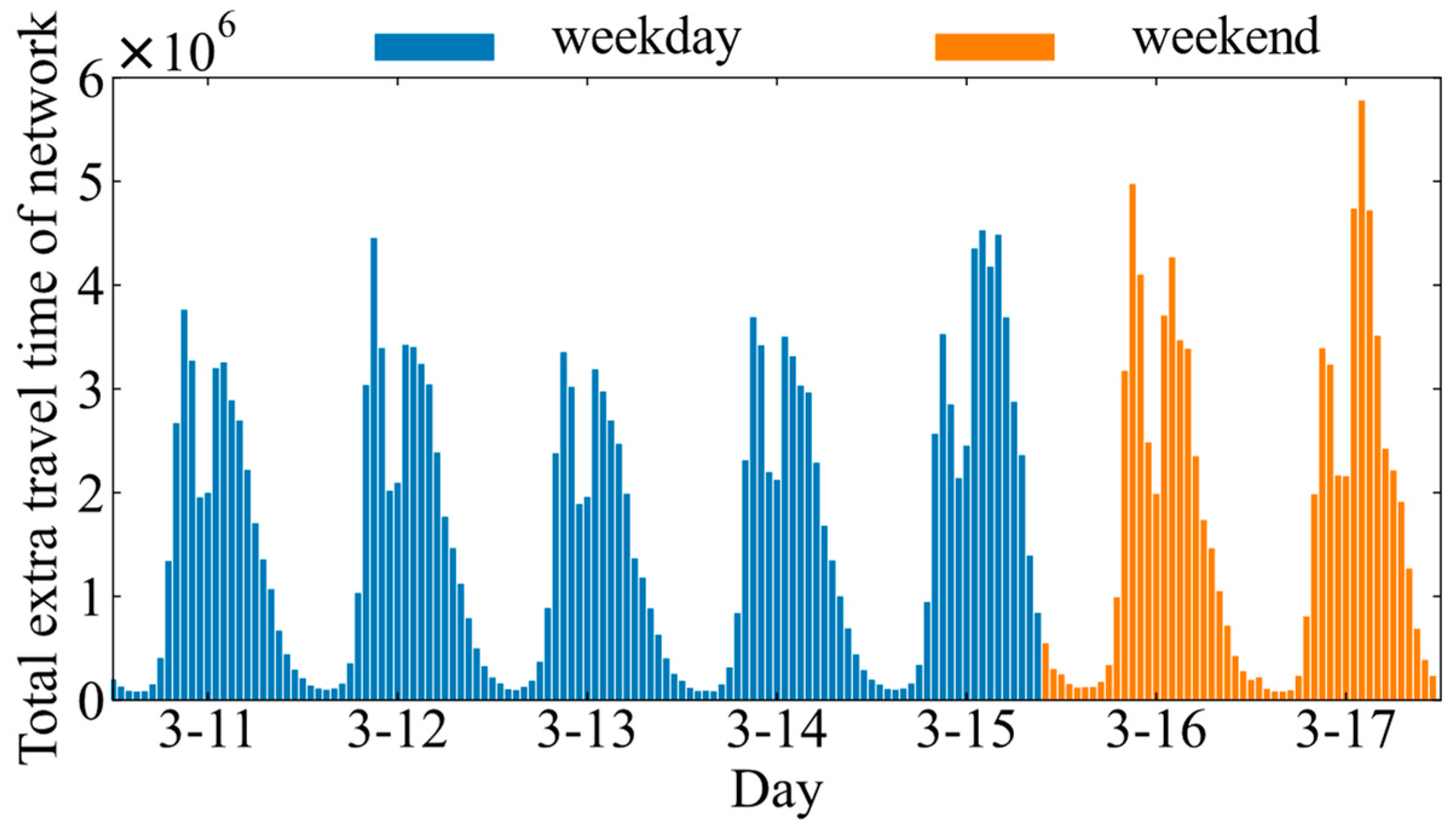
To understand the emergence of congestion driver sources, we first analyzed the spatiotemporal patterns of extra travel times. We calculated the total extra travel time on the freeway network during each one-hour time window (Figure 6). We found that the network-wide extra travel time showed a morning peak and an afternoon peak, which is consistent with the temporal patterns of travel demand. This is not surprising because large travel demand is the fundamental driving force of traffic congestion and longer travel time. As shown in Figure 6, the largest extra travel time was observed on Sunday afternoon, which is when many travelers return to their workplace or home from their weekend journeys.
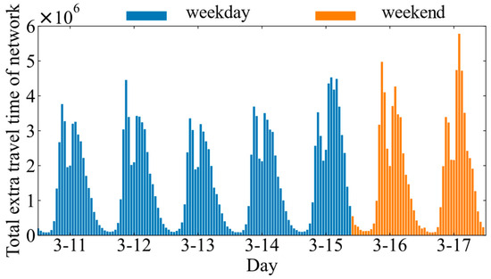
Figure 6.
The temporal distribution of extra travel time of the freeway network.
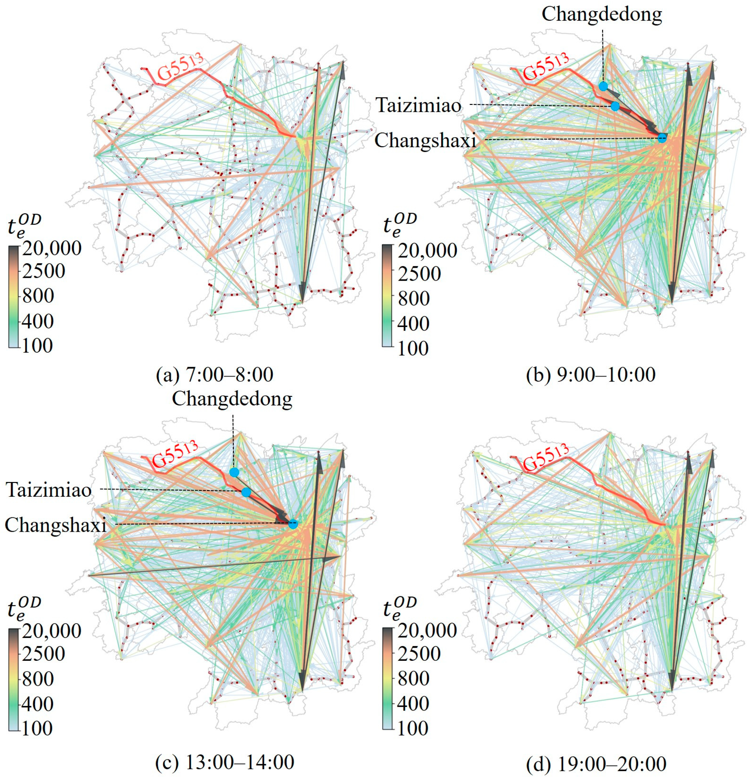
As shown in Figure 7, the O-D pairs with large extra travel times are mainly distributed on the G5513 Changsha–Zhangjiajie freeway, implying that the freeway capacity cannot accommodate the large travel demand well. In addition, large extra travel times are also observed between some toll stations near the border of Hunan province. This is consistent with our intuition that trips on these O-D pairs are long-distance trips passing through many congested freeway sections. Finally, some O-D pairs with their origins or destinations located in Changsha are characterized by large extra travel times. Interestingly, the extra travel times of some O-D pairs show tidal pattern. For example, the extra travel time from Changshaxi toll station to Taizimiao toll station is longer during the morning peak hour, whereas the extra travel time is longer in the opposite direction during the afternoon peak hour (Figure 7).
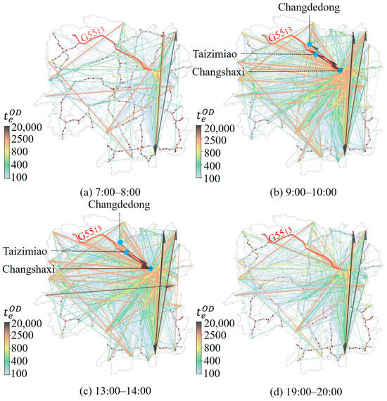
Figure 7.
The average extra travel times of O-D pairs in four time windows (7:00 a.m.–8:00 a.m., 9:00 a.m.–10:00 a.m., 13:00 p.m.–14:00 p.m., and 19:00 p.m.–20:00 p.m.) from 11 March to 17 March 2019.
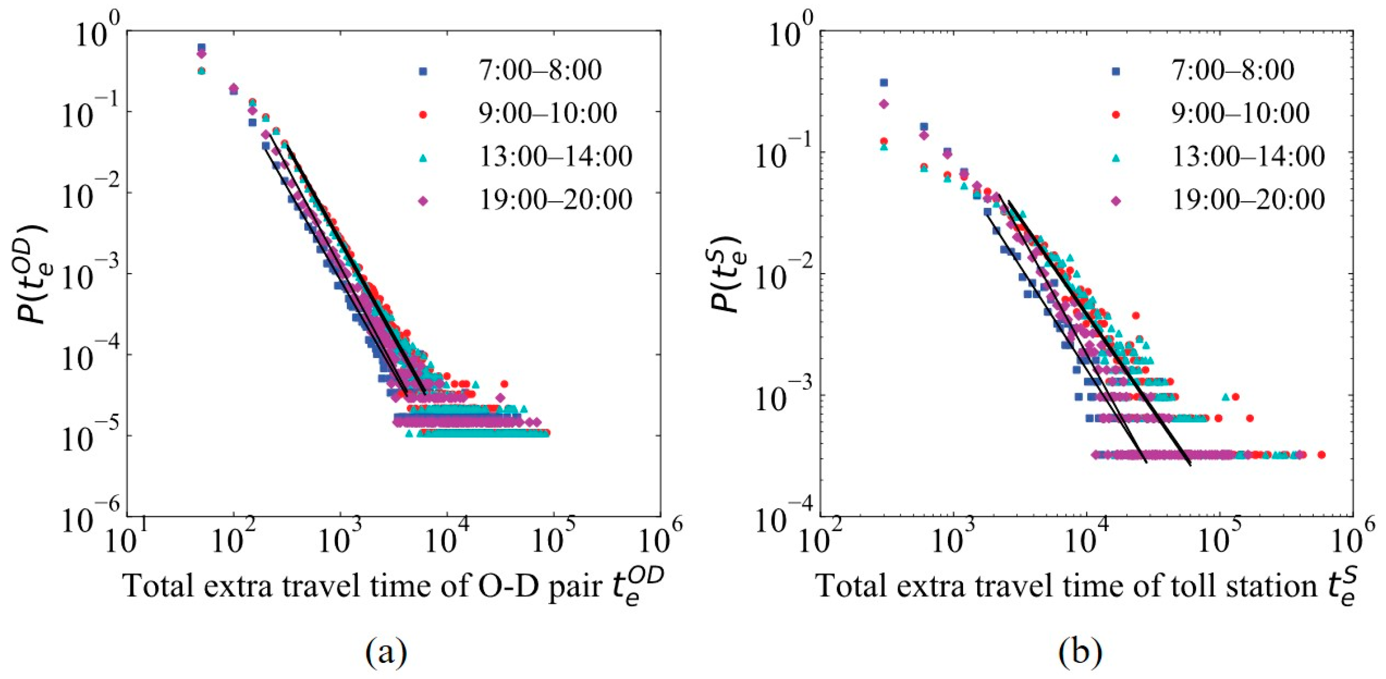
As shown in Figure 8, both the extra travel times of O-D pairs and the extra travel times of toll stations follow power law distributions. The heterogeneously distributed extra travel time originates from the heterogeneously distributed travel demand. This finding implies that drivers from most driver sources enjoy a relatively high level of service, while drivers from a few driver sources suffer large extra travel time and contribute to major traffic congestion. The heterogeneously distributed extra travel time also suggests that we can pinpoint a small number of CDSs that cause major traffic congestion.
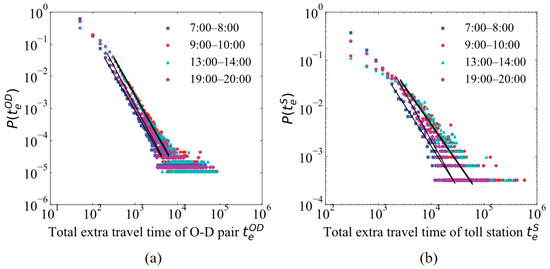
Figure 8.
Distribution of the average extra travel times of (a) O-D pairs and (b) toll stations in four time windows.
4.2. Spatiotemporal Patterns of Congestion Driver Sources
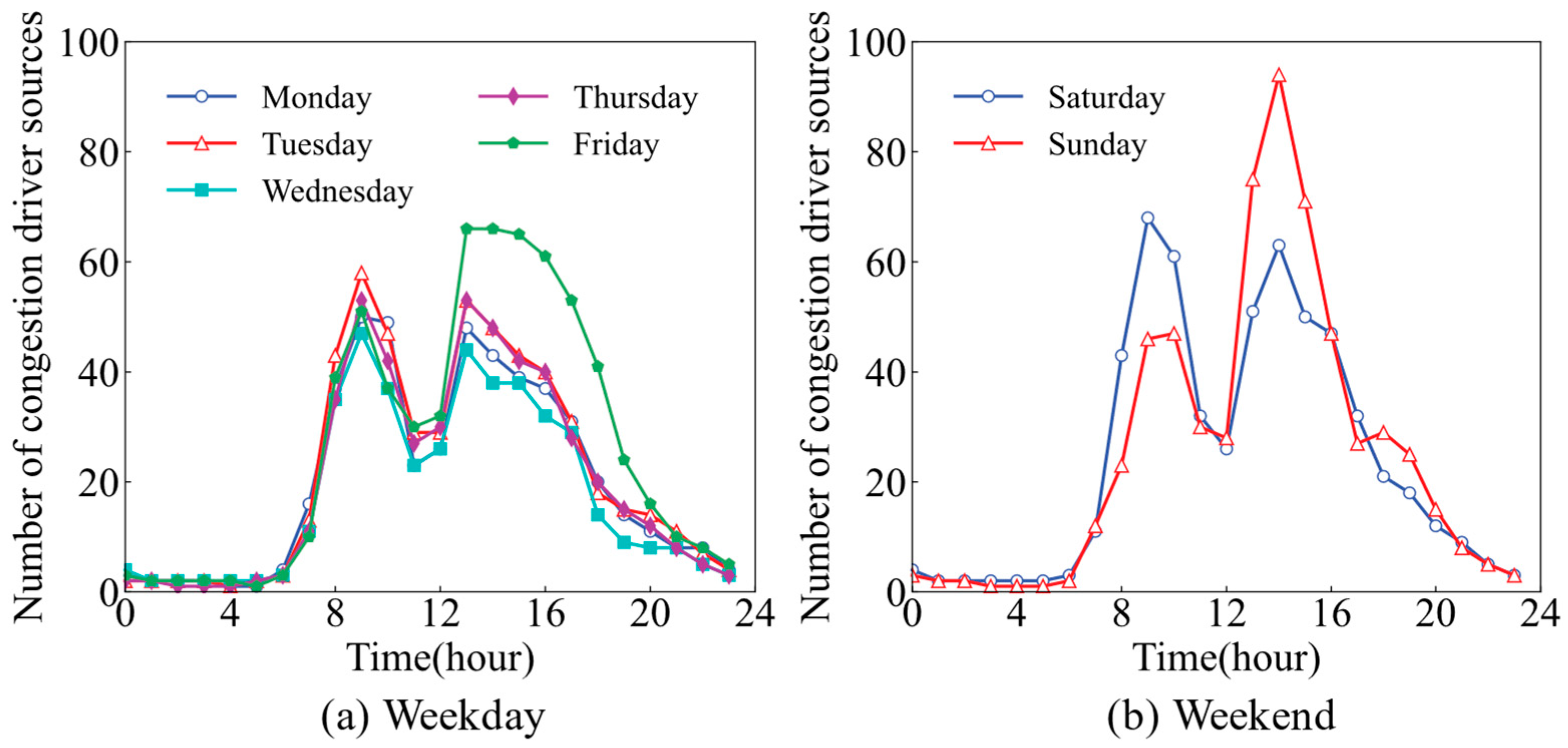
We used the method proposed in Section 3.2 to identify the congestion driver sources (CDSs) during each one-hour time window from 11 March 2019 to 17 March 2019. We observed similar temporal patterns of CDSs across the five weekdays and the two weekend days (Figure 9). The number of CDSs had two peaks in the morning and afternoon, respectively, which is consistent with the temporal patterns of travel demand and extra travel time. During a weekday, a toll station is identified as a CDS for an average of 1.15 h. In particular, the number of CDSs exhibits a prominent increase on Friday evening, which could have been generated by the early weekday journeys (Figure 9a). During a weekend day, a toll station is identified as a CDS for an average of 1.32 h. There are more CDSs on Saturday morning, which could be caused by the weekday journeys (Figure 9b). Compared with the weekday afternoons, there are more CDSs on Sunday afternoon, which could have been generated by the weekend returning trips.
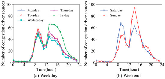
Figure 9.
The number of CDSs in the Hunan freeway network during each one-hour time window from 11 March 2019 to 17 March 2019.
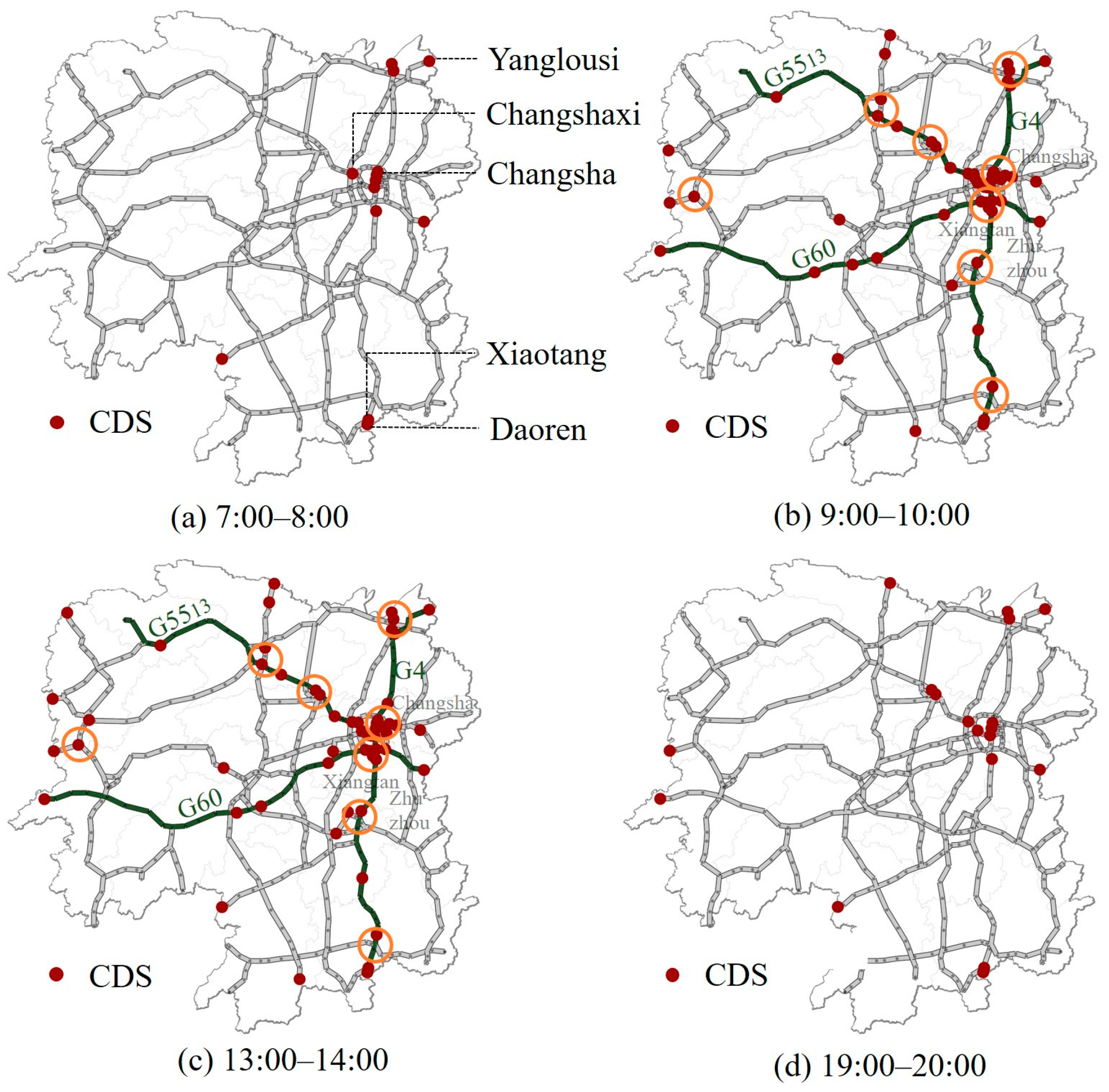
We further analyzed the spatial distribution of congestion driver sources (CDSs) (Figure 10). We found that during off-peak hours, the CDSs were mainly distributed at the toll stations located at the border of Hunan province and some toll stations located at the peripheral area of Changsha (Figure 10a,d). Alternatively, during peak hours, CDSs were additionally observed at some toll stations near the freeway interconnecting hubs (see the orange circles in Figure 10b,c). The CDSs located at the province border were generated by the long-distance trips passing through many congested freeway sections. The average travel time of vehicles from the provincial boundary toll stations (152 min) was much longer than the network-wide average value (51 min). The CDSs around Changsha were caused by the strong attraction of the core city to travelers from other cities in Hunan province. The CDSs located near the freeway interconnecting hubs were caused by the large merging traffic flows of different freeways. Importantly, the spatial distribution of CDSs was pretty stable during the peak hours and off-peak hours, suggesting that transportation agencies can focus on a small number of CDSs and deploy targeted traffic control strategies to mitigate traffic congestion [27,28].
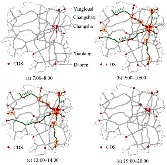
Figure 10.
The spatial distribution of CDSs in the Hunan freeway network during different time windows. Solid red circles represent the congestion driver sources. Orange circles represent the freeway interconnecting hubs. Green lines represent the freeways.
5. Major Driver Sources of Local Freeway Sections
Identifying the major driver sources of a local freeway section also provides useful information for traffic control and transportation management. For example, if a freeway section is the bottleneck of the freeway network, which often suffers severe traffic congestion, locating its major driver sources (MDSs) can facilitate travel demand control upstream. Similarly, identifying the MDSs of a freeway section where traffic accidents or road maintenance works occur (usually reducing the capacity of the section) can pinpoint the drivers whose trips will be influenced. Transportation agencies can suggest alternative routes to potentially affected drivers [37], send an alert to them [38], or postpone their entering onto the freeway [39]. In the following, we identify the MDSs of two case study freeway sections.
5.1. Major Driver Sources of a Freeway Section with a Traffic Accident
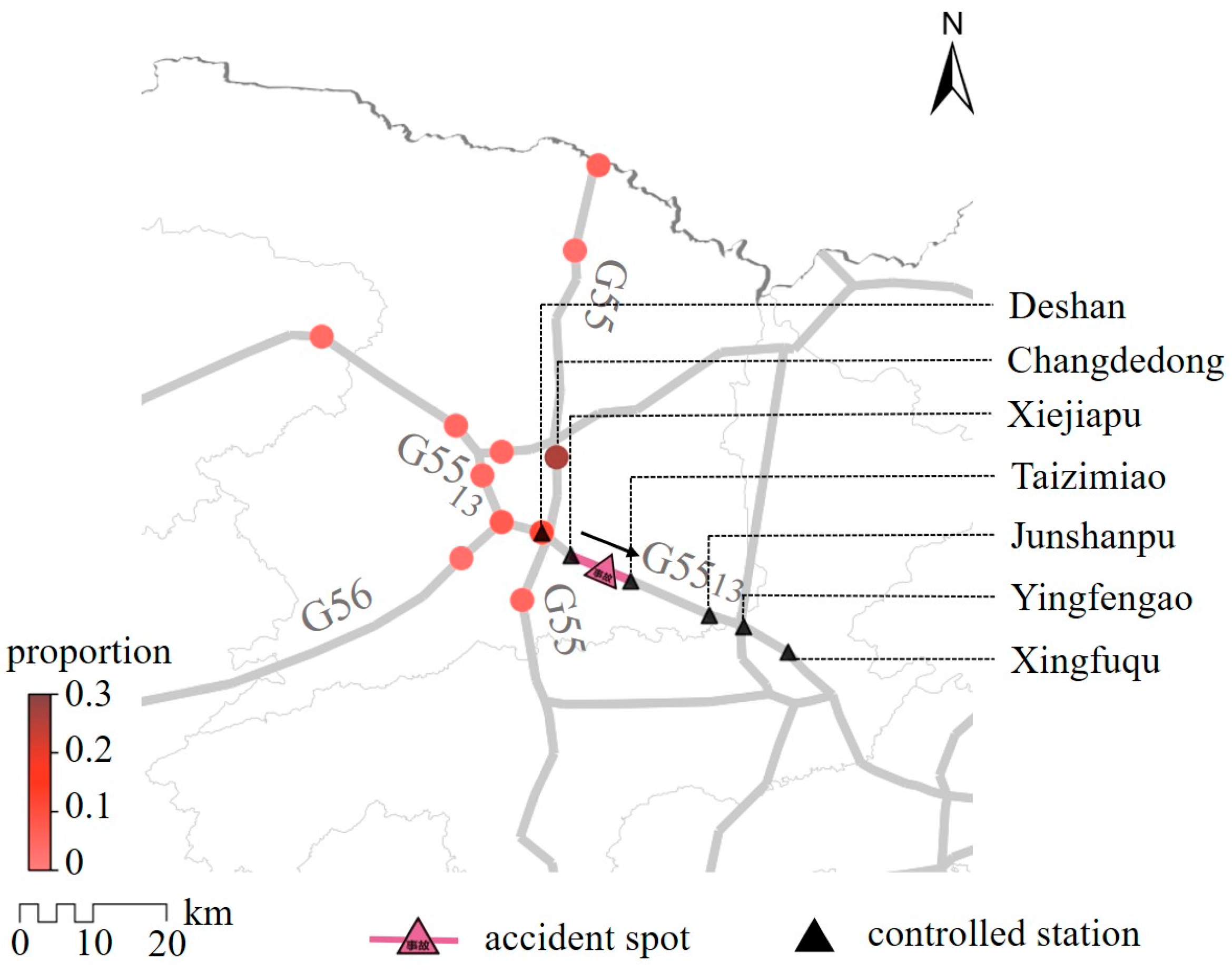
At about 20:00 p.m., 22 March 2019, a severe traffic accident occurred on a freeway section near the Taizimiao toll station on the west-to-east direction of the G5513 Changsha–Zhangjiajie freeway. During the time window from 20:00 p.m. to 21:00 p.m., the MDSs of the freeway section were mainly distributed at the toll stations on the G55 Erenhot–Guangzhou freeway and G5513 Changsha–Zhangjiajie freeway (Figure 11). Among the identified MDSs, the Changdedong and Deshan toll stations together contribute 38% of the traffic flow of the freeway section. However, the transportation agency implemented temporary traffic control at the Xingfuqu, Yingfengqiao, Junshanpu, Taizimiao, Xiejiapu, and Deshan toll stations, most of which were not the MDSs of the freeway section and were located downstream of the accident. The vehicles passing through the accidental location were not controlled due to the lack of MDS information. This highlights the importance of identifying the MDSs of local freeway sections.
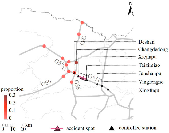
Figure 11.
The MDSs of the freeway section where a traffic accident occurred on 22 March 2019. Red dots represent the major driver sources.
5.2. Major Driver Sources of a Freeway Section under Maintenance Work
From 9 April 2019 to 30 April 2019, the S71 Nanxian–Yiyang freeway from Yingfengqiao toll station to Yuanjiangnan toll station was closed for maintenance. During this period, the Yuanjiangnan toll station only allowed vehicles that were entering but did not allow vehicles that were exiting. Figure 12 illustrates the MDSs of the freeway section under maintenance during the time window from 13:00 p.m. to 14:00 p.m. on April 15. Six toll stations were identified as the MDSs, in which Changshaxi toll station was the driver source contributing the most traffic flow (26%). Interestingly, the identified MDSs were not distributed in the vicinity of the studied freeway section, and some driver sources were far from the freeway section. Identifying MDSs can help to locate the travelers whose trips will be influenced by freeway maintenance work and help them to plan alternative routes.
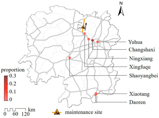
Figure 12.
The MDSs of a freeway section under maintenance during the time window of 13:00 p.m.–14:00 p.m. on 15 April 2019. Red dots represent the major driver sources.
6. Discussion
An interesting question is whether the spatial distribution of CDSs is consistent with the topological importance of toll stations. Here, we used three typical centrality measures (i.e., betweenness centrality, closeness centrality, and degree centrality) to analyze the topological importance of nodes (including the 449 toll stations) in the studied freeway network. Specifically, the betweenness centrality of a node denotes the number of shortest paths passing through the node, the closeness centrality denotes the average distance from the node to the other nodes, and the degree centrality denotes the number of edges connected to the node [40,41]. As shown in Figure 13, the spatial distributions of CDSs have no obvious correlation with their topological importance, highlighting the important role of travel demand in determining the spatial distribution of CDSs.
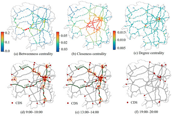
Figure 13.
The topological importance of nodes in the studied freeway network measured by the betweenness centrality (a), the closeness centrality (b), and the degree centrality (c). The spatial distribution of CDSs in the Hunan freeway network during different time windows (d–f). Solid red circles represent the congestion driver sources. Orange circles represent the freeway interconnecting hubs. Green lines represent the freeways.
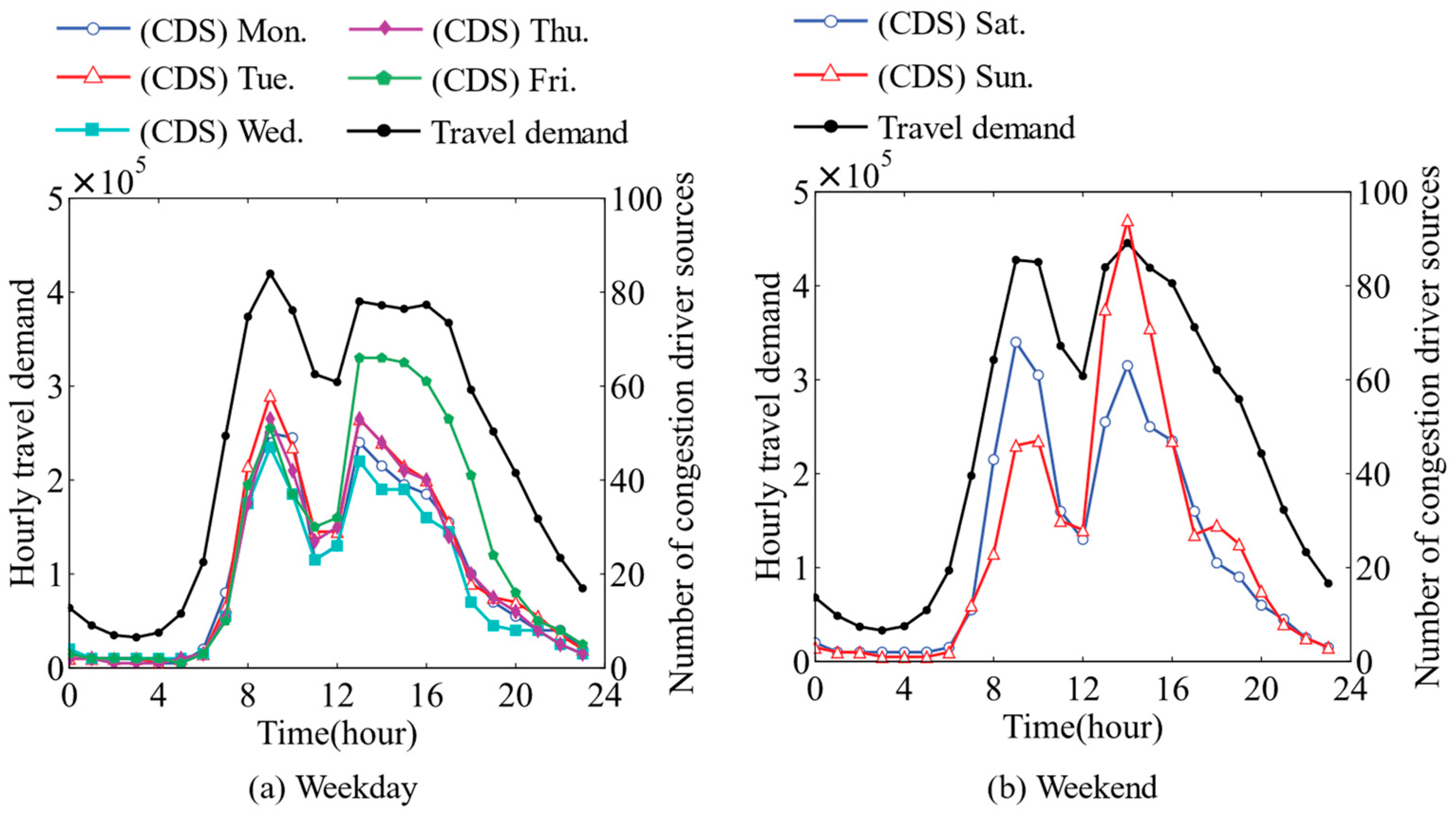
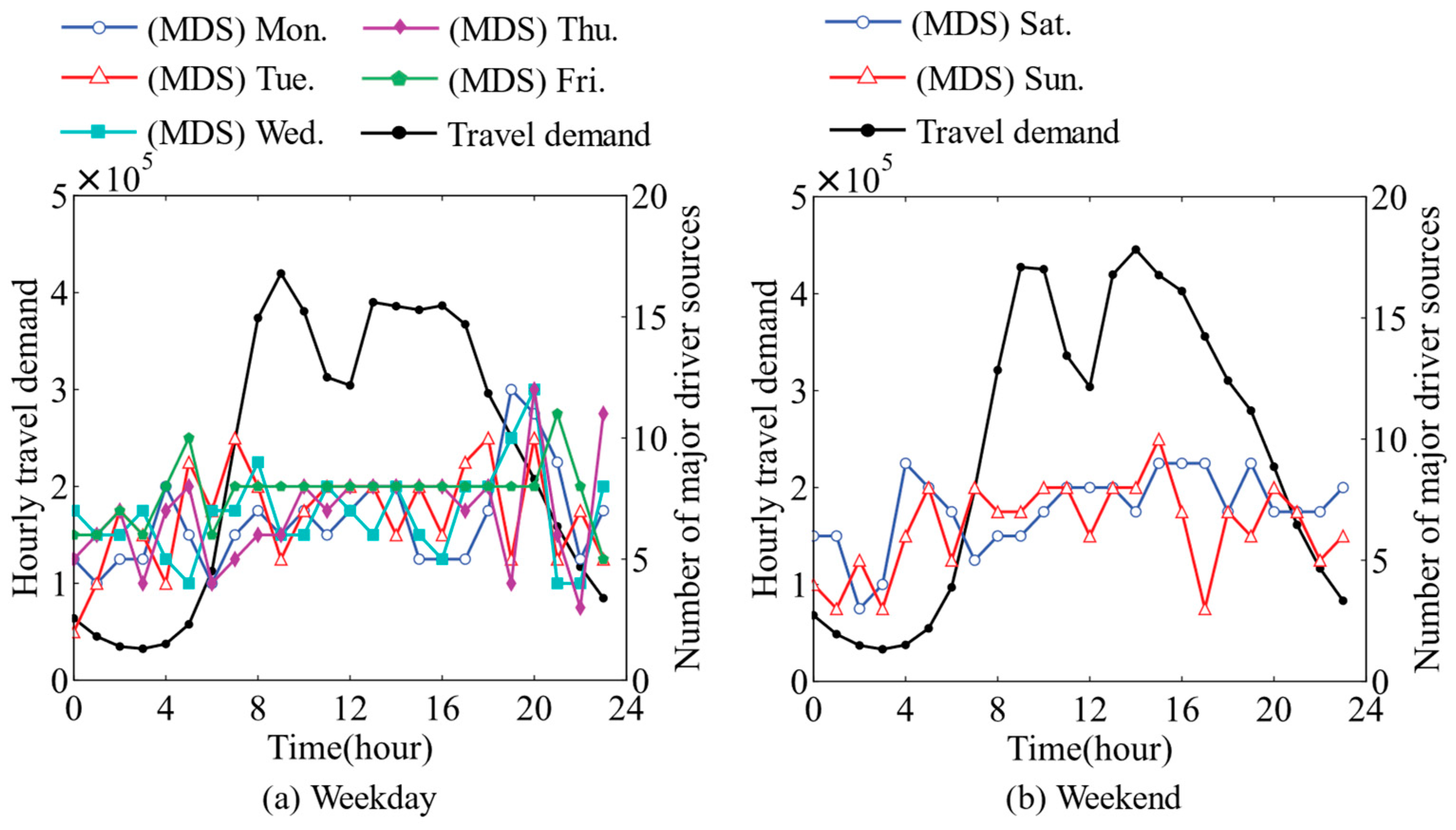
Next, we explored the temporal correlation between the number of CDSs and MDSs and the travel demand. We found that the number of CDSs changed with the travel demand accordingly (Figure 14). The strong correlation between the number of CDSs and the travel demand was further validated by measuring the Pearson and Spearman correlation coefficients between them (Table 2). To analyze the temporal patterns of MDSs, we used the G0421 Xuchang–Guangzhou freeway from Shebu toll station to Huilongqiao toll station as a case study freeway section. However, the correlation between the number of MDSs and the freeway travel demand was much weaker (Figure 15, Table 3).
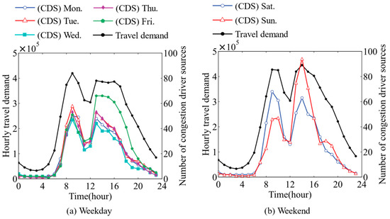
Figure 14.
The number of CDSs in the Hunan freeway network and the average number of freeway trips during each one-hour time window from 11 March 2019 to 17 March 2019.
Table 2.
Pearson and Spearman correlation coefficients between the number of CDSs and the travel demand.
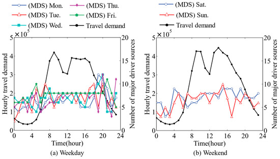
Figure 15.
The number of MDSs of a case study freeway section and the average number of freeway trips during each one-hour time window from 11 March 2019 to 17 March 2019.
Table 3.
Pearson and Spearman correlation coefficients between the number of MDSs and the travel demand.
7. Conclusions
In this study, we have proposed a new K-PSO-algorithm-based method to identify the congestion driver sources (CDSs) of the freeway network and the major driver sources (MDSs) of local freeway sections. Using freeway travel demand data, we analyzed the spatiotemporal patterns of CDSs and MDSs. Locating the CDSs can assist transportation agencies in identifying the major origins of traffic congestion. The results indicate that the congestion driver sources are mostly observed during heavy traffic periods and mainly distributed in the regions surrounding Changsha and the regions adjacent to other provinces and freeway interconnecting hubs. Locating the MDSs of local freeway sections can help transportation agencies to identify the travelers whose trips could be potentially affected by traffic accidents or road maintenance works, facilitating the development of effective countermeasures. The proposed method and the discovered spatiotemporal patterns of CDSs and MDSs contribute to both freeway congestion mitigation and freeway emergency responses, both of which are crucial for the development of sustainable regional transportation systems.
The present study has some limitations, which calls for future investigations. We only analyzed the spatiotemporal patterns of CDSs and MDSs under regular traffic conditions based on relatively coarse travel demand data. In future studies, the spatiotemporal distributions of CDSs and MDSs during holidays and bad weather can be further analyzed. Moreover, vehicle trajectory data can be used to simulate real-time traffic flow and locate the CDSs and MDSs at a higher temporal resolution. Finally, the obtained CDS and MDS information can assist transportation agencies in deploying more targeted traffic control strategies, which could improve the congestion mitigation effect and reduce the cost of implementing traffic control schemes.
Author Contributions
Conceptualization, P.W.; methodology, B.W. and H.Y.; data curation, B.W., S.L. and J.D.; writing—original draft preparation, B.W. and R.K.; writing—review and editing, H.Y. and P.W.; visualization, B.W. and R.K.; supervision, P.W. and J.D. All authors have read and agreed to the published version of the manuscript.
Funding
This work was supported by the Hunan Provincial Natural Science Fund for Distinguished Young Scholars [grant number: 2022JJ10077] and the 2021 Science and Technology Progress and Innovation Plan of Department of Transportation of Hunan province [grant number: 202102].
Institutional Review Board Statement
Not applicable.
Informed Consent Statement
Not applicable.
Data Availability Statement
The data are not publicly available due to the confidentiality agreement.
Acknowledgments
The authors thank T. Wang, Y. Liao, and S. Lv for valuable discussions.
Conflicts of Interest
Author Jianjun Dai was employed by the company Hunan Communications Research Institute Co., Ltd. The remaining authors declare that the research was conducted in the absence of any commercial or financial relationships that could be construed as a potential conflict of interest.
References
- Ignatov, A. European highway networks, transportation costs, and regional income. Reg. Sci. Urban Econ. 2024, 104, 103969. [Google Scholar] [CrossRef]
- Saha, P.; Sarkar, A.K.; Pal, M. Evaluation of speed–flow characteristics on two-lane highways with mixed traffic. Transport 2017, 32, 331–339. [Google Scholar] [CrossRef]
- Cao, S.; Xu, H.; Xu, Y.; Wang, X.; Zheng, Y.; Li, Y. Assessment of the integrated benefits of highway infrastructure and analysis of the spatiotemporal variation: Evidence from 29 provinces in China. Socio-Econ. Plan. Sci. 2023, 90, 101740. [Google Scholar] [CrossRef]
- Ministry of Transport of the People’s Republic of China. Statistical Communiqué of the People’s Republic of China on the 2012 Highway and Waterway Transport Industry Development. 2013. Available online: https://www.mot.gov.cn/fenxigongbao/hangyegongbao/201510/t20151013_1894759.html (accessed on 28 February 2024).
- Ministry of Transport of the People’s Republic of China. Statistical Communiqué of the People’s Republic of China on the 2022 Transport Industry Development. 2023. Available online: https://xxgk.mot.gov.cn/2020/jigou/zhghs/202306/t20230615_3847023.html (accessed on 28 February 2024).
- Outwater, M.; Tierney, K.; Bradley, M.; Sall, E.; Kuppam, A.; Modugula, V. California statewide model for high-speed rail. J. Choice Model. 2010, 3, 58–83. [Google Scholar] [CrossRef]
- Department of Transportation of Huan Province. Statistical Communiqué of the Hunan Province on the 2017 Highway and Waterway Transport Industry Development. 2018. Available online: https://jtt.hunan.gov.cn/xxgk/zwgg/201804/t20180402_4983863.html (accessed on 28 February 2024).
- Department of Transportation of Huan Province. Statistical Communiqué of the Hunan Province on the 2022 Highway and Waterway Transport Industry Development. 2023. Available online: https://jtt.hunan.gov.cn/jtt/xxgk/jttj/202307/t20230725_29410204.html (accessed on 28 February 2024).
- Yuan, M.; Mai, J.; Liu, X.; Shen, H.; Wang, J. Current Implementation and Development Countermeasures of Green Energy in China’s Highway Transportation. Sustainability 2023, 15, 3024. [Google Scholar] [CrossRef]
- Jing, T.; Liu, D.; Bao, Y.; Wang, H.; Yan, M.; Zu, F. Spatiotemporal Distributions and Vulnerability Assessment of Highway Blockage under Low-Visibility Weather in Eastern China Based on the FAHP and CRITIC Methods. Atmosphere 2023, 14, 756. [Google Scholar] [CrossRef]
- Retallack, A.E.; Ostendorf, B. Relationship between traffic volume and accident frequency at intersections. Int. J. Environ. Res. Public Health 2020, 17, 1393. [Google Scholar] [CrossRef]
- Zhang, L.; Levinson, D. Optimal freeway ramp control without origin–destination information. Transp. Res. Part B Methodol. 2004, 38, 869–887. [Google Scholar] [CrossRef]
- Grumert, E.; Ma, X.; Tapani, A. Analysis of a cooperative variable speed limit system using microscopic traffic simulation. Transp. Res. Part C Emerg. Technol. 2015, 52, 173–186. [Google Scholar] [CrossRef]
- Vreeswijk, J.D.; Landman, R.L.; van Berkum, E.C.; Hegyi, A.; Hoogendoorn, S.P.; van Arem, B. Improving the road network performance with dynamic route guidance by considering the indifference band of road users. IET Intell. Transp. Syst. 2015, 9, 897–906. [Google Scholar] [CrossRef]
- Jun, J. Understanding the variability of speed distributions under mixed traffic conditions caused by holiday traffic. Transp. Res. Part C Emerg. Technol. 2010, 18, 599–610. [Google Scholar] [CrossRef]
- Chen, Y.; Chen, C.; Wu, Q.; Ma, J.; Zhang, G.; Milton, J. Spatial-temporal traffic congestion identification and correlation extraction using floating car data. J. Intell. Transp. Syst. 2021, 25, 263–280. [Google Scholar] [CrossRef]
- Yang, Y.; Li, M.; Yu, J.; He, F. Expressway bottleneck pattern identification using traffic big data—The case of ring roads in Beijing, China. J. Intell. Transp. Syst. 2020, 24, 54–67. [Google Scholar] [CrossRef]
- Sarvi, M.; Kuwahara, M.; Ceder, A. Observing freeway ramp merging phenomena in congested traffic. J. Adv. Transp. 2010, 41, 145–170. [Google Scholar] [CrossRef]
- Fernando, R. The impact of Planned Special Events (PSEs) on urban traffic congestion. EAI Endorsed Trans. Scalable Inf. Syst. 2019, 6, e4. [Google Scholar] [CrossRef]
- Pei, Y.; Cai, X.; Li, J.; Song, K.; Liu, R. Method for identifying the traffic congestion situation of the main road in cold-climate cities based on the clustering analysis algorithm. Sustainability 2021, 13, 9741–9771. [Google Scholar] [CrossRef]
- Ren, J.; Chen, Y.; Xin, L.; Shi, J.; Li, B.; Liu, Y. Detecting and positioning of traffic incidents via video-based analysis of traffic states in a road segment. IET Intell. Transp. Syst. 2016, 10, 428–437. [Google Scholar] [CrossRef]
- Ghosh, L.E.; Abdelmohsen, A.; El-Rayes, K.A.; Ouyang, Y. Temporary traffic control strategy optimization for urban freeways. Transp. Res. Rec. 2018, 2672, 68–78. [Google Scholar] [CrossRef]
- Zhang, T.; Guo, G. Graph attention LSTM: A spatiotemporal approach for traffic flow forecasting. IEEE Intell. Transp. Syst. Mag. 2020, 14, 190–196. [Google Scholar] [CrossRef]
- Guo, G.; Yuan, W.; Liu, J.; Lv, Y.; Liu, W. Traffic forecasting via dilated temporal convolution with peak-sensitive loss. IEEE Intell. Transp. Syst. Mag. 2021, 15, 48–57. [Google Scholar] [CrossRef]
- Guo, G.; Zhang, T. A residual spatio-temporal architecture for travel demand forecasting. Transp. Res. Part C Emerg. Technol. 2020, 115, 102639. [Google Scholar] [CrossRef]
- Wang, P.; Hunter, T.; Bayen, A.M.; Schechtner, K.; González, M.C. Understanding road usage patterns in urban areas. Sci. Rep. 2012, 2, 1001. [Google Scholar] [CrossRef]
- Li, M.; Yang, H.; Guo, B.; Dai, J.; Wang, P. Driver Source-Based Traffic Control Approach for Mitigating Congestion in Freeway Bottlenecks. J. Adv. Transp. 2022, 2022, 3536979. [Google Scholar] [CrossRef]
- Li, S.; Yang, H.; Li, M.; Dai, J.; Wang, P. A Highway On-Ramp Control Approach Integrating Percolation Bottleneck Analysis and Vehicle Source Identification. Sustainability 2023, 15, 12608. [Google Scholar] [CrossRef]
- Wang, C.; Xu, Z.; Du, R.; Li, H.; Wang, P. A vehicle routing model based on large-scale radio frequency identification data. J. Intell. Transp. Syst. 2020, 24, 142–155. [Google Scholar] [CrossRef]
- Zhang, J.; Yan, X.; An, M.; Sun, L. The impact of Beijing subway’s new fare policy on riders’ attitude, travel pattern and demand. Sustainability 2017, 9, 689. [Google Scholar] [CrossRef]
- He, Z. Spatial-temporal fractal of urban agglomeration travel demand. Phys. A Stat. Mech. Its Appl. 2020, 549, 124503. [Google Scholar] [CrossRef]
- Sun, C.; Jing, H.; Chen, T.; Li, M.; Zhang, P. Incremental equilibrium assignment and applications to traffic network model. IET Intell. Transp. Syst. 2023, 17, 794–803. [Google Scholar] [CrossRef]
- Xu, M.H.; Liu, Y.Q.; Huang, Q.L.; Zhang, Y.X.; Luan, G.F. An improved Dijkstra’s shortest path algorithm for sparse network. Appl. Math. Comput. 2007, 185, 247–254. [Google Scholar] [CrossRef]
- Wang, S.; Huang, W.; Lu, Z. Deduction of link performance function and its regression analysis. J. Highw. Transp. Res. Dev. 2006, 23, 107–110. [Google Scholar]
- Zhao, Y.; Lu, J.; Zhang, W.; Sun, X. Improvement effect analysis of congestion pricing using Logit model. J. Public Transp. 2017, 49, 80–85. [Google Scholar]
- Ruan, Y.; Chen, J.; Fan, Z.; Wang, T.; Mu, J.; Huo, R.; Huang, W.; Liu, W.; Li, Y.; Sun, Y. Application of K-PSO Clustering Algorithm and Game Theory in Rock Mass Quality Evaluation of Maji Hydropower Station. Appl. Sci. 2023, 13, 8467. [Google Scholar] [CrossRef]
- Rezaei, M.; Noori, H.; Razlighi, M.M.; Nickray, M. Refocus+: Multi-layers real-time intelligent route guidance system with congestion detection and avoidance. IEEE Trans. Intell. Transp. Syst. 2019, 22, 50–63. [Google Scholar] [CrossRef]
- Jindahra, P.; Choocharukul, K. Short-run route diversion: An empirical investigation into variable message sign design and policy experiments. IEEE Trans. Intell. Transp. Syst. 2012, 14, 388–397. [Google Scholar] [CrossRef]
- Haule, H.J.; Alluri, P.; Sando, T. Mobility impacts of ramp metering operations on freeways. J. Transp. Eng. Part A Syst. 2022, 148, 04021109. [Google Scholar] [CrossRef]
- Liu, Z.; Jiang, C.; Wang, J.; Yu, H. The node importance in actual complex networks based on a multi-attribute ranking method. Knowl.-Based Syst. 2015, 84, 56–66. [Google Scholar] [CrossRef]
- Zhao, S.; Zhao, P.; Cui, Y. A network centrality measure framework for analyzing urban traffic flow: A case study of Wuhan, China. Phys. A Stat. Mech. Appl. 2017, 478, 143–157. [Google Scholar] [CrossRef]


Disclaimer/Publisher’s Note: The statements, opinions and data contained in all publications are solely those of the individual author(s) and contributor(s) and not of MDPI and/or the editor(s). MDPI and/or the editor(s) disclaim responsibility for any injury to people or property resulting from any ideas, methods, instructions or products referred to in the content. |
© 2024 by the authors. Licensee MDPI, Basel, Switzerland. This article is an open access article distributed under the terms and conditions of the Creative Commons Attribution (CC BY) license (https://creativecommons.org/licenses/by/4.0/).