4.1. Differences in the Spatial and Temporal Distribution of Carbon Intensity
Firstly, carbon intensity within the western region was calculated by comparing carbon emissions to GDP. Temporal variations in carbon intensity were visually depicted using Origin 2021 software, with point and line maps created to illustrate fluctuation trends over time. Furthermore, spatial differences in carbon intensity were illustrated through regional grading utilizing ArcGIS 10.2 software, as demonstrated in
Figure 2 and
Figure 3.
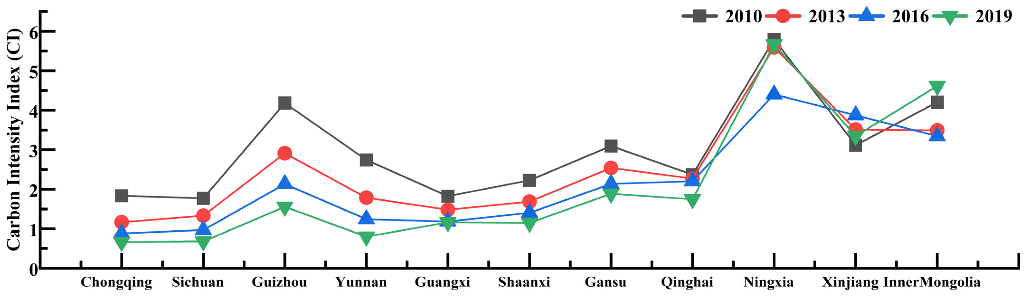
As depicted in
Figure 2, the overall temporal trend of carbon intensity demonstrates a year-on-year decrease. However, specific localities exhibit notable fluctuations, particularly in Ningxia, Xinjiang, and Inner Mongolia.
In Ningxia, the carbon intensity initially experiences a decline, followed by an upward shift. The most significant fluctuation in carbon intensity occurred between 2013 and 2016, with a subsequent decreasing trend. In Xinjiang, there is an initial increase in carbon intensity, succeeded by a decline. The period from 2016 to 2019 witnessed the most substantial fluctuation in carbon intensity, followed by a decreasing trend. Inner Mongolia, conversely, displays an initial decrease in carbon intensity, succeeded by a subsequent rise. The years from 2016 to 2019 witnessed a noticeable increase in carbon intensity fluctuations. In contrast, the remaining western regions consistently exhibited a decreasing trend in carbon intensity year after year.
Over a broad temporal scale, the annual reduction in carbon intensity reflects China’s progress in enhancing energy efficiency and transitioning towards a low-carbon economy. This progress is likely associated with a suite of national-level energy-saving and emission-reduction policies, along with technological innovations. Despite the general trend of declining carbon intensity, the trends in Ningxia, Xinjiang, and Inner Mongolia reveal significant inter-regional differences. These discrepancies may be attributed to variations in economic structure, energy configuration, industrial layout, and technological levels across regions [
41,
42,
43,
44]. Therefore, policy formulation needs to take into account regional economic and energy structure characteristics in order to design low-carbon development strategies that are appropriate to local realities.
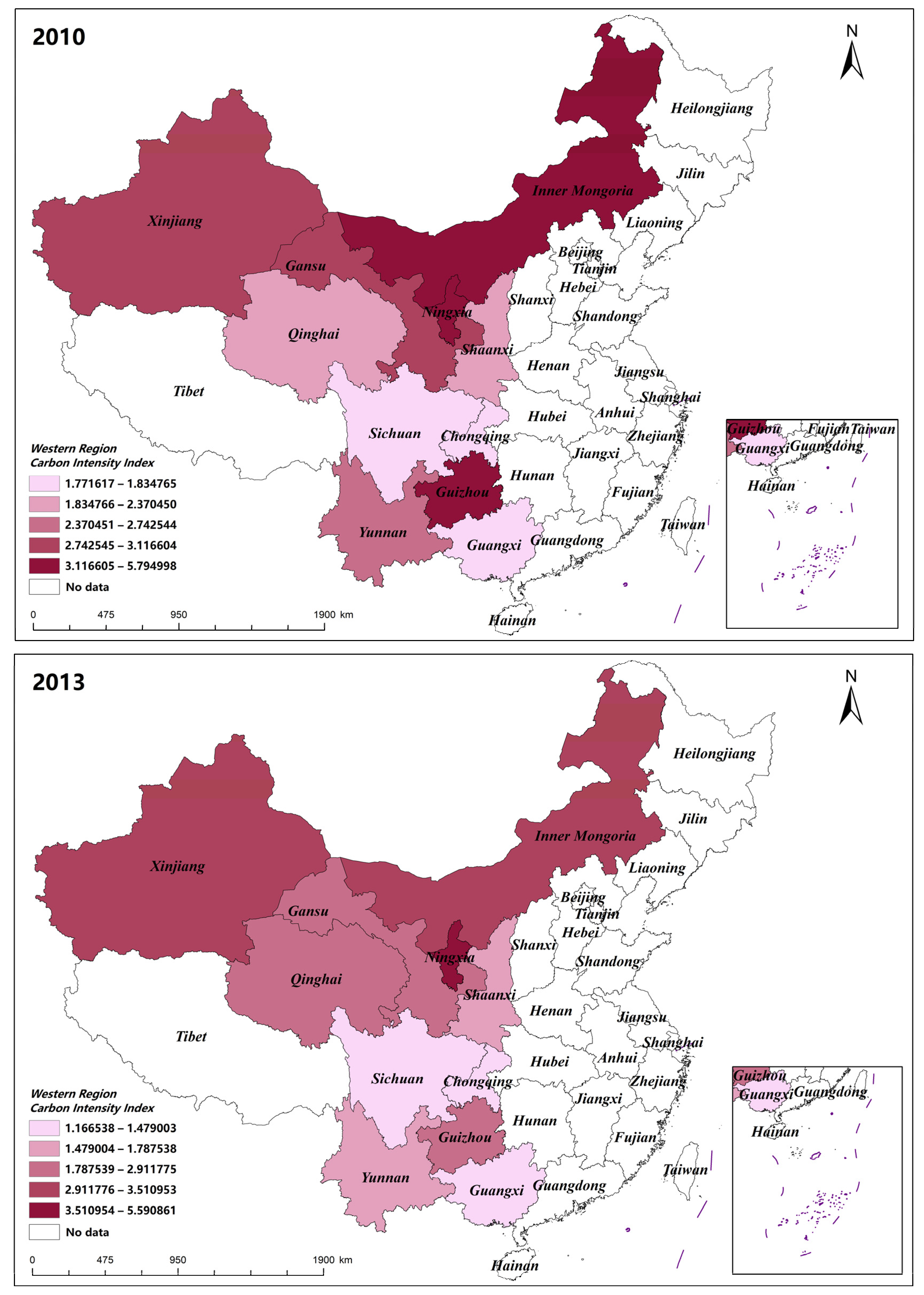
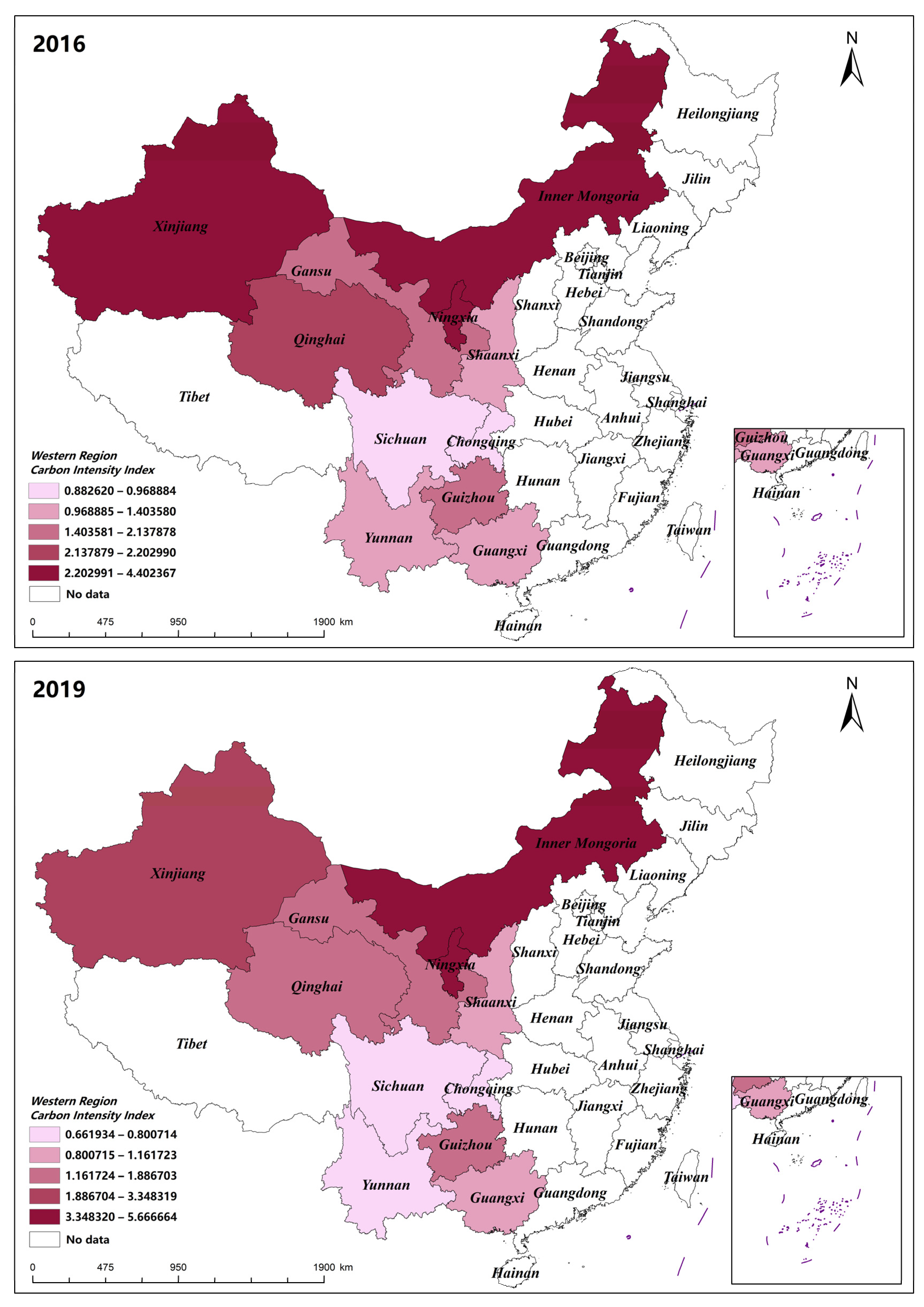
Figure 3 illustrates a distinct concentration of carbon intensity in the western region, particularly evident with higher levels in the north-central compared to the southern part. Notably, a consistent year-by-year decline in carbon intensity is observed.
In the year 2010, the Inner Mongolia Autonomous Region, the Ningxia Hui Autonomous Region, and Guizhou Province exhibited notably elevated levels of carbon intensity. During this period, carbon emissions were approximately 5 to 6 times the respective regional GDP. This emphasizes a significant carbon footprint associated with the developmental activities in these regions. The high carbon intensity underscores the intricate relationship between economic development and heightened carbon emissions within these areas. In 2013, a comparison with 2010 revealed relatively stable carbon emissions in the Ningxia Hui Autonomous Region. Despite the stability, carbon intensity remained persistently high. Concurrently, Inner Mongolia and Guizhou experienced a transition from high to medium carbon intensity levels during this period.
Moving to 2016, there was a general decline in carbon intensity across all western regions, except for Xinjiang and Inner Mongolia, where levels remained relatively stable. Notably, in 2019, Inner Mongolia is anticipated to experience a rebound in carbon intensity, while other regions are expected to maintain their existing levels with no significant changes. This temporal analysis underscores the dynamic nature of carbon emissions, reflecting both stability and fluctuations in different regions over the specified time frame.
The distribution of carbon intensity exhibits different trends over time and space. This distribution may be attributed to factors such as industrial structure, energy consumption patterns, economic development levels, and geographical and climatic conditions [
44,
45]. The northern region’s reliance on heavy industry and fossil fuels such as coal likely contributes to its elevated carbon intensity. However, the entire western region demonstrates a year-over-year declining trend in carbon intensity, indicating progress in enhancing energy efficiency and reducing carbon emissions. This progress is likely due to national initiatives for green, low-carbon development, adjustments in the energy structure, and the application of clean energy technologies [
46].
4.2. Analysis of Temporal Factors Influencing Carbon Intensity
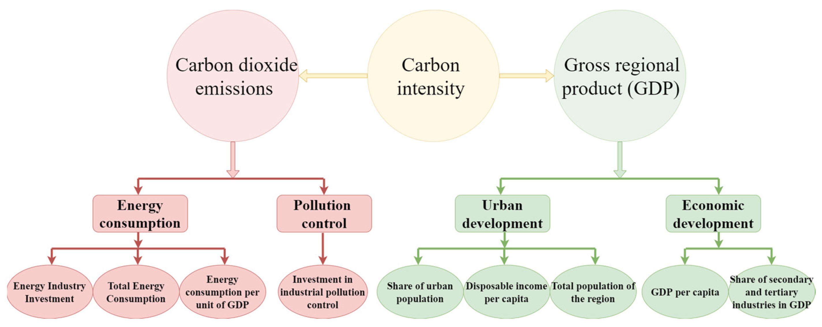
The STIRPAT model was employed to analyze the influencing factors depicted in
Figure 1, identifying the determinants of carbon intensity over time in the western regions. The operational procedure of the STIRPAT model begins with the identification of significant factors that impact carbon intensity. This is followed by an analysis of collinearity using ordinary least squares (OLS). Finally, ridge regression analysis is conducted based on the significance analysis and ordinary least squares analysis.
The chosen variables undergo a rigorous scientific selection process, where significant independent variables are selected using the stepwise regression forward and backward method. As depicted in
Table 1, the resulting variables GDP per capita, energy industry investment, disposable income per capita, total energy consumption, energy consumption per unit of GDP, and investment in industrial pollution control exhibit potential relationships with the dependent variable. To delve deeper, linear regression was employed to further validate these relationships.
Based on the findings of the significance analysis, GDP per capita, energy industry investment, disposable income per capita, total energy consumption, energy consumption per unit of GDP, and investment in industrial pollution control were selected as independent variables, with carbon intensity serving as the dependent variable for analysis using ordinary least squares (OLS). The results are presented in
Table 2. The model successfully passed the F-test (F = 517.676,
p = 0.000 < 0.05), indicating that at least one of GDP per capita, energy industry investment, disposable income per capita, total energy consumption, energy consumption per unit of GDP, and investment in industrial pollution control significantly influences carbon intensity. The study examined the relationships between GDP value, energy industry investment, disposable income per capita, total energy consumption, energy consumption per unit of GDP, and industrial pollution control investment amount, to determine their impact on carbon intensity. Additionally, a multiple covariance test applied to the model identified a VIF (Variance Inflation Factor) value exceeding 10 for energy industry investment, signaling a covariance issue. This indicates that the coefficients obtained from the results of the ordinary least squares fitting cannot be reliably guaranteed, and, consequently, cannot serve as a solid scientific foundation.
To mitigate the interference resulting from the multiple covariances inherent in panel data, and to preserve a more substantial amount of information from both the independent variables and the dependent variable, the ridge regression method was adopted for data analysis. This approach addresses the challenges posed by multiple covariance interference in panel data analysis while maximizing the retention of critical information from the independent and dependent variables. To effectively address the issue of multiple covariance interference in panel data and better preserve the information contained in the independent and dependent variables, the data were reanalyzed using the ridge regression method.
The ridge regression program was implemented using SPSS 25.0 software. The analysis involved equations, ridge trace plots, and goodness-of-fit assessments across various values of the ridge parameter (k). The independent variables included per capita GDP, energy industry investment, per capita disposable income of residents, total energy consumption, energy consumption per unit of GDP, and investment in the treatment of industrial pollution. Carbon intensity was the designated dependent variable.
Upon setting k = 0.05, the ridge coefficients exhibited stabilization, and the model’s R-squared value reached 0.983. This indicates that per capita GDP, energy industry investment, per capita disposable income, total energy consumption, energy consumption per unit of GDP, and investment in industrial pollution control collectively explain 98.3% of the variance in carbon intensity. Detailed results of the ridge regression at k = 0.05 are presented in
Table 3. Furthermore, the model underwent an F-test, yielding a statistically significant result (F = 37.766,
p = 0.002 < 0.05). This implies that at least one of the variables, namely per capita GDP, energy industry investment, disposable income per capita, total energy consumption, energy consumption per unit of GDP, or industrial pollution control investment, significantly influences the relationship with carbon intensity. The non-standard coefficient equation derived from ridge regression aligns with the STIRPAT model equation.
where
denotes carbon intensity;
is GDP per capita,
is energy industry investment,
is disposable income per capita,
is total energy consumption,
is energy consumption per unit of GDP, and
is investment in industrial pollution control.
The regression analysis reveals noteworthy findings regarding the impact of various factors on carbon intensity. Specifically: The regression coefficient for per capita GDP is 1.256 (t = 3.378, p = 0.028 < 0.05), indicating a significant positive influence on carbon intensity. Energy industry investment is associated with a regression coefficient of −0.810 (t = −3.120, p = 0.036 < 0.05), signifying a significant negative impact on carbon intensity. Per capita disposable income exhibits a regression coefficient of −2.753 (t = −3.813, p = 0.019 < 0.05), suggesting a significant negative effect on carbon intensity. Total energy consumption’s regression coefficient is 0.172 (t = 0.582, p = 0.592 > 0.05), implying a non-significant positive impact on carbon intensity. The regression coefficient for energy consumption per unit of GDP is 2.611 (t = 12.409, p = 0.000 < 0.01), indicating a significant positive influence on carbon intensity. Industrial pollution control investment is associated with a regression coefficient of 0.956 (t = 4.360, p = 0.012 < 0.05), signifying a significant positive impact on carbon intensity.
Results derived from the STIRPAT model indicate that per capita GDP, energy consumption per unit of GDP, and investment in industrial pollution control significantly contribute to the increase in carbon intensity. Conversely, investment in the energy sector and per capita disposable income are associated with a significant reduction in carbon intensity. In this analysis, total energy consumption does not have a statistically significant impact on carbon intensity. Per capita GDP’s rise is tied to higher carbon intensity, suggesting economic growth’s environmental toll. Clean energy investments are inversely related to carbon intensity, indicating efficiency gains. Higher incomes align with greener consumption, aiding emission cuts. Energy use per GDP unit reflects efficiency deficits in high-intensity economies. Despite pollution control investments suggesting increased industrial activity, a holistic strategy promoting sustainable growth, clean energy, and low-carbon habits is key to reducing carbon intensity, with policy evaluations needing to account for complex economic-social dynamics.
4.3. Analysis of Factors Affecting Carbon Intensity in the Spatial Dimension
The Geo-detector model was utilized to analyze the influencing factors illustrated in
Figure 1, precisely identifying the determinants of carbon intensity within the spatial dimension of the western regions. Initially, the reclassification tool in ArcGIS was employed to convert the original continuous data raster. Subsequent calculations were performed in Excel 2016, with the Geo-detector 2015 software acting as a macro within the Excel spreadsheet to directly process the data for analysis. The outcomes included both univariate and bivariate analyses. The results of the univariate and bivariate analyses are detailed in
Table 4 and
Table 5.
From the results of the Single-factor analysis of variance (
Table 4), it is evident that energy consumption per unit of GDP and the total regional population exerts a more substantial explanatory influence on the spatial variation of carbon intensity in the western region. Particularly noteworthy is the average explanatory power of energy consumption per unit of GDP, which attains 0.755, signifying the highest degree of impact on the spatial differentiation of carbon intensity. Conversely, the category with the least explanatory power regarding the spatial distribution differences in carbon intensity is the proportion of secondary and tertiary industries to GDP, registering an average explanatory power of 0.095. Assessing the level of influence, it is discerned that energy consumption and urban development wield a more pronounced effect on carbon intensity.
The results of the two-factor analysis of variance (
Table 5) reveal that the impact of two-factor interaction on the spatial differentiation of carbon intensity in the western region surpasses that of a single factor, demonstrating non-linear enhancement and two-factor synergies. In 2010, the most robust interaction effect occurred between the proportion of urban population and energy consumption per unit of GDP, yielding an explanatory power of 0.996. This underscores that changes in the urban population proportion and energy consumption per unit of GDP were the primary driving forces behind the spatial variation in carbon intensity. In 2013, the interaction between total regional population and GDP per capita exhibited the highest level of influence, boasting an explanatory power of 0.996. This suggests that the total regional population and GDP per capita played pivotal roles in shaping the spatial distribution of carbon intensity. Similar to 2013, 2016 witnessed the most potent interaction between the total regional population and GDP per capita, registering an explanatory power of 1.000. The paramount two-factor explanatory power in 2019 was associated with the total regional population and urban population share, with an explanatory power of 0.998.
In summary, the explanatory power of two-factor interactions during the period 2010–2019 spans from the proportion of urban population and energy consumption per unit of GDP to the total regional population and GDP per capita, and ultimately to the total regional population and the proportion of urban population. The dynamic evolution of interaction explanatory power suggests that the primary influence on spatial variation in carbon intensity stems from the interaction between energy consumption and urban development.
The rationale behind the observed spatial variance in carbon intensity being impacted by energy consumption and urban development may lie in the fact that energy serves as a fundamental indicator of economic development. Simultaneously, energy consumption directly results in carbon emissions, influencing both GDP values and carbon emissions, thereby affecting carbon intensity. Moreover, cities and towns represent focal points of human activities, and their developmental levels directly impact regional economies. The processes associated with human activities contribute to carbon emissions, further influencing carbon intensity. Consequently, the interaction between energy consumption and urban development, as core factors influencing carbon intensity, emerges as the central explanatory power for spatial disparities in carbon intensity distribution.
Results obtained using the Geo-detector model reveal that in the univariate analysis, energy consumption per unit of GDP and Disposable income per capita exert the strongest influence on the spatial variation of carbon intensity. Bivariate interaction analysis discloses that the proportion of the proportion of the urban population and energy consumption per unit of GDP, as well as the Total population and per capita GDP, have the most pronounced impact on the spatial variation of carbon intensity at different time intervals.
4.4. Projections of Spatial and Temporal Development of Carbon Intensity
This study employs raw data related to carbon intensity in the western regions from 2010 to 2021 and utilizes the GM (1:1) grey prediction model to forecast the development of carbon intensity. With the assistance of MATLAB 2019a software, Equations (6)–(9) are applied to process the raw data, yielding predicted values for the carbon intensity development in the western regions. Precision testing and error analysis of the development forecast are conducted (see
Table 6 for detailed criteria), resulting in a Small Error Probability Test (
p) value of 1, and Variance Ratio Test (C) values of 0.032, 0.028, 0.014, 0.028, 0.050, 0.025, 0.017, 0.086, 0.183, 0.155, and 0.157, respectively. Through rigorous accuracy testing and error analysis, the prediction model demonstrates high precision.
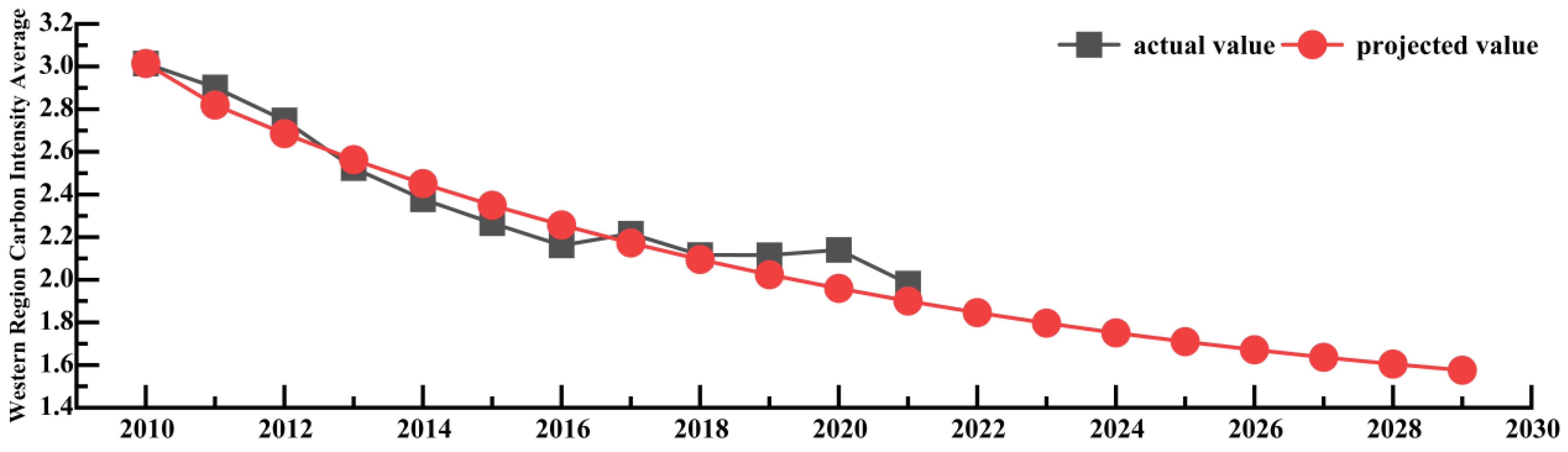
As evident from
Figure 4, the actual average carbon intensity for the western regions in 2021 was 2.14. This indicates that the total carbon emissions were 2.14 times the Gross Domestic Product (GDP) of the region, highlighting the correlation between regional economic development and an increase in carbon emissions. The outcomes of the prediction model reveal a yearly decreasing trend in regional average carbon intensity. The predicted average carbon intensity for 2029 stands at 1.576, suggesting a declining ratio between the economy and the environment. This implies a reduction in environmental loss during economic development and an enhancement in environmental protection benefits throughout the economic construction process.
Building on the analysis of factors influencing the spatio temporal distribution of carbon intensity, the current trend in the average actual carbon intensity in the western regions is affected by energy consumption per unit of GDP, per capita GDP, investment in industrial pollution control, investment in the energy sector, per capita disposable income, and the urban population ratio. Model predictions suggest that from 2021 to 2029, the average carbon intensity in the western regions is expected to decrease annually by 7.01%. Compared to the national target set in the “14th Five-Year Plan” of reducing carbon intensity by 65% by 2030 relative to 2005 levels, the current trajectory appears promising. To maintain this positive trend in carbon intensity, it is imperative to address and reinforce the temporal and spatial factors influencing it. Policy recommendations should stem from these factors, including energy consumption per unit of GDP, per capita GDP, investment in industrial pollution control, investment in the energy sector, per capita disposable income, and the urban population ratio.


