

Tugboat Scheduling Method Based on the NRPER-DDPG Algorithm: An Integrated DDPG Algorithm with Prioritized Experience Replay and Noise Reduction


Abstract
1. Introduction
2. Literature Review
2.1. Tug Dispatching Method
2.2. Reinforcement Learning Scheduling Method
3. Problem Description
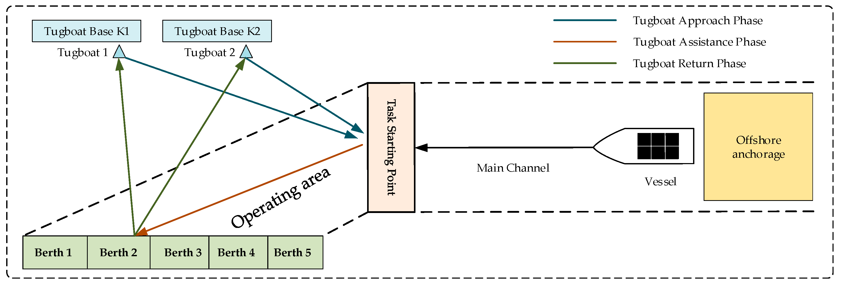
3.1. Tugboat Scheduling Process
3.2. Problem Hypothesis
- (1)
- The start and end times of each task are fixed and not influenced by random factors.
- (2)
- All relevant information about the task, including the required number of tugboats, power ratings, and task duration, is available before scheduling the tugboats.
- (3)
- The location of the tugboat base where the tugboats are docked is known before the start of all tasks.
- (4)
- The time taken by tugboats to dock and depart from the base is negligible compared to their transit time.
- (5)
- Different tugboats have their respective fixed speed (optimal economic speed).
- (6)
- Each tugboat base has an upper limit on the number of tugboats it can accommodate.
3.3. Symbol Definition
3.4. Mathematical Model
3.5. Model Processing
4. Improved DDPG Algorithm
4.1. Markov Decision Process
4.2. State Space Definition
4.3. Action Space Definition
4.4. Reward Setting
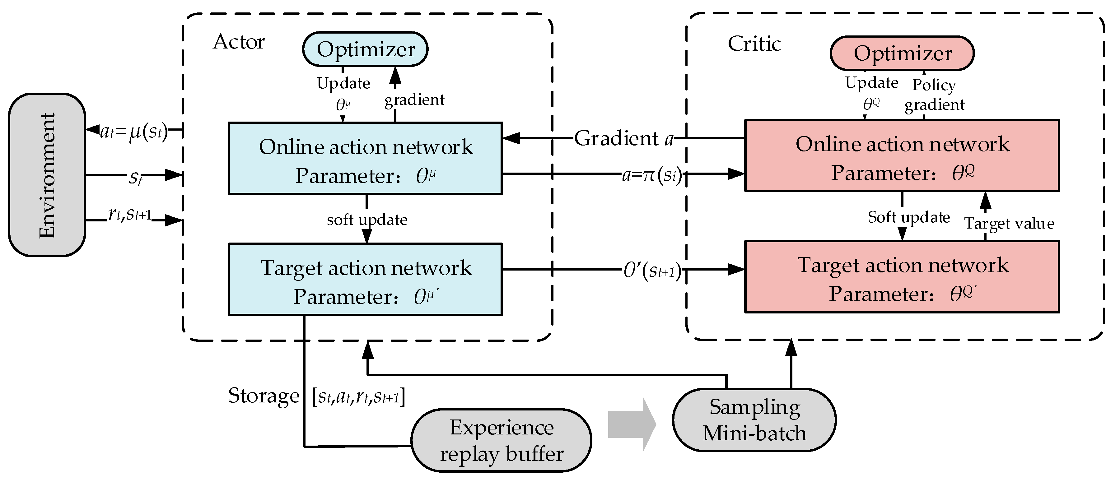
4.5. DDPG Algorithm
4.6. Prioritized Experience Replay Mechanism
4.7. Noise Reduction Method
4.8. Tugboat Scheduling Method Based on the NRPER-DDPG Algorithm
- (1)
- Acquisition of Port Task-Related Information: Firstly, information related to port tasks is obtained, including the arrival time of each task, the required number of tugboats, expected working hours, and specific tugboat power requirements. Subsequently, detailed data on the existing tugboats in the port are collected, covering the number of tugboats, power, idle speed, idle cost, and assistance cost, as well as the number and specific geographical location of tugboat bases, to initialize the tugboat scheduling environment.
- (2)
- Initialization of Experience Replay Buffer: Experience samples are constructed from information related to decision-making, such as state, action, and reward, and the experience replay buffer is initialized. Subsequently, these experience samples are added to the buffer by randomly generating initial solutions, ensuring that the agent interacts with the environment to generate new experiences and provide more learning samples.
- (3)
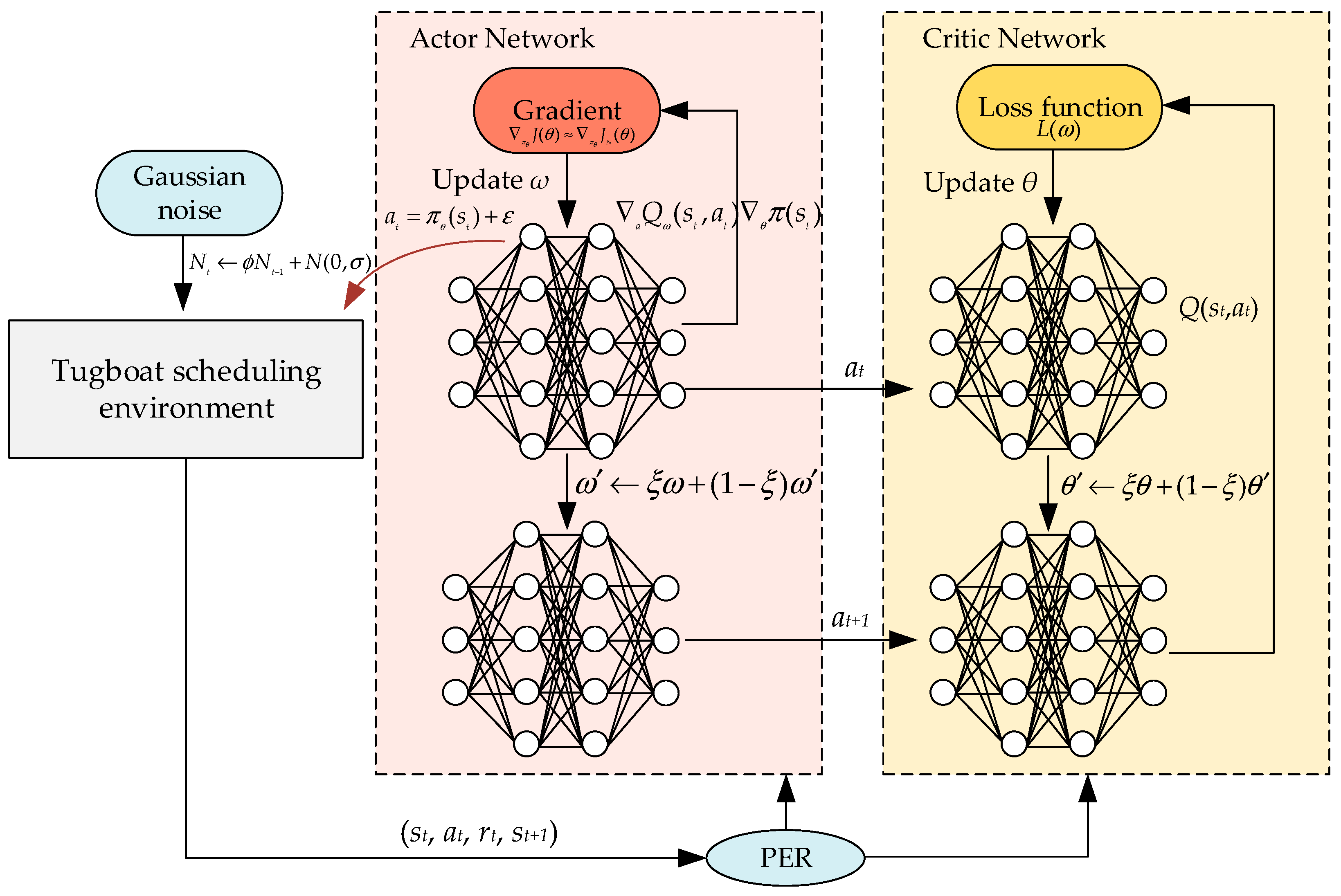
- Actor-Critic Network Model Training: The Actor network receives environmental state information as input and outputs tugboat actions. Noise is introduced into the action output to improve exploration. Meanwhile, the environmental state information and the action information generated by the Actor network are used as inputs to the Critic network, which estimates the value of the actions. The output of the Critic network is an estimate of the value function for a given state and action, and this output is used to calculate the TD error for prioritized experience replay.
- (4)
- Iterative Optimization of Reinforcement Learning Model: The deep reinforcement learning model based on the Actor-Critic network is trained to learn which actions to take in different states to maximize cumulative rewards. This involves adjusting decisions such as tugboat task allocation and departure times to optimize fuel costs and task completion times. After multiple iterations of training, the model continuously optimizes the tugboat scheduling strategy.
| Algorithm 1. Tugboat Scheduling Method Using the NRPER-DDPG Algorithm |
| Initialize: tugboat scheduling environment, parameters for Actor and Critic networks, experience replay buffer ReplayBuffer, noise parameters |
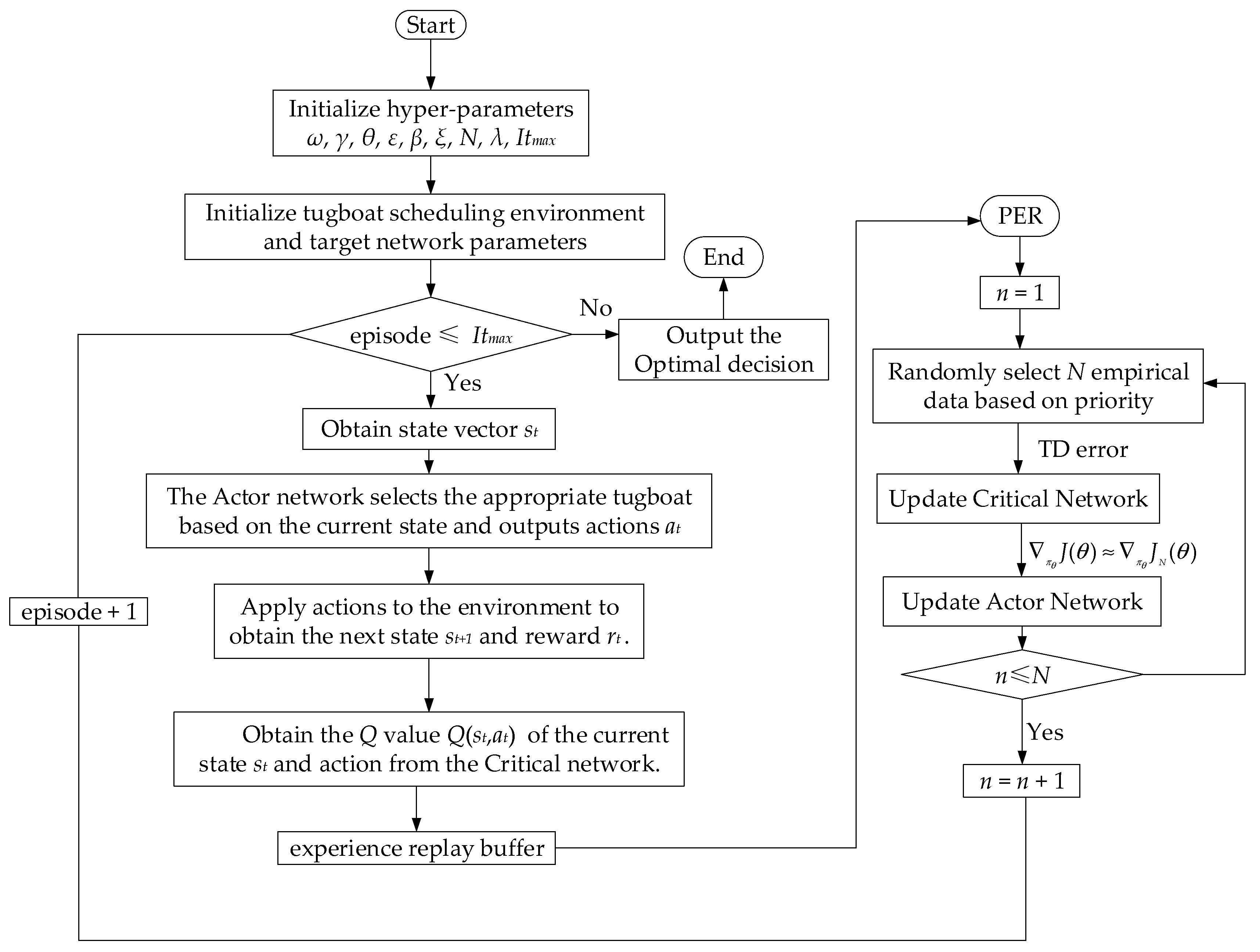
| Input: hyper-parameters ω, γ, θ, ε, β, ξ, N, λ, Itmax |
| Output: Tugboat scheduling decision |
| For episode in range(Itmax): |
| Initialize state s |
| For step in range(max_steps): |
| The Actor target network approximates the next action value based on the current state st |
| Target Q-values = Critic_target(st + 1, a) |
| Store state transition sequence [st, at, rt, st + 1] to the experience replay memory |
| Update priority function using the current Q-values output by Critic |
| If replay_buffer is full: |
| Randomly sample a minibatch of transitions [st, at, rt, st + 1] from replay_buffer |
| Compute target Q-values y_target using Critic_target |
| Calculate the mean square error loss function |
| Update Critic neural network |
| Using Small Batch Gradient Descent Method to Calculate the Maximum Value of J(θ) |
| Update Actor neural network |
| If episode % update_freq = 0: |
| Soft update target networks Actor_target and Critic_target |
| Decay noise to a smaller value |
| s = st + 1 |
5. Experimental Discussion
5.1. Experimental Parameter Settings
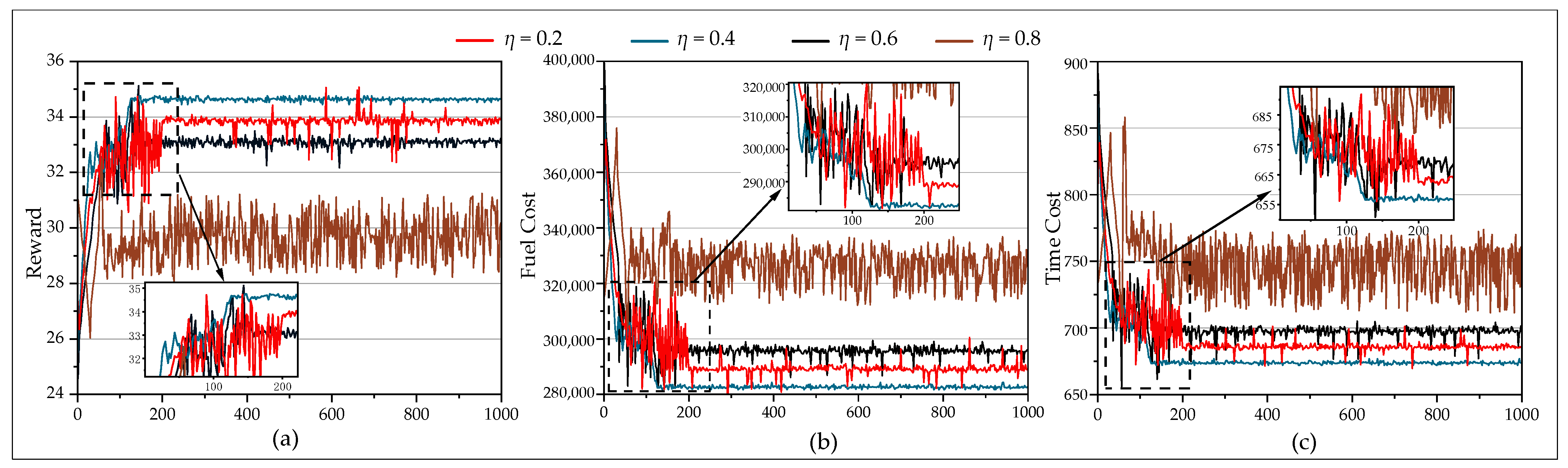
5.2. Parameter Experiments
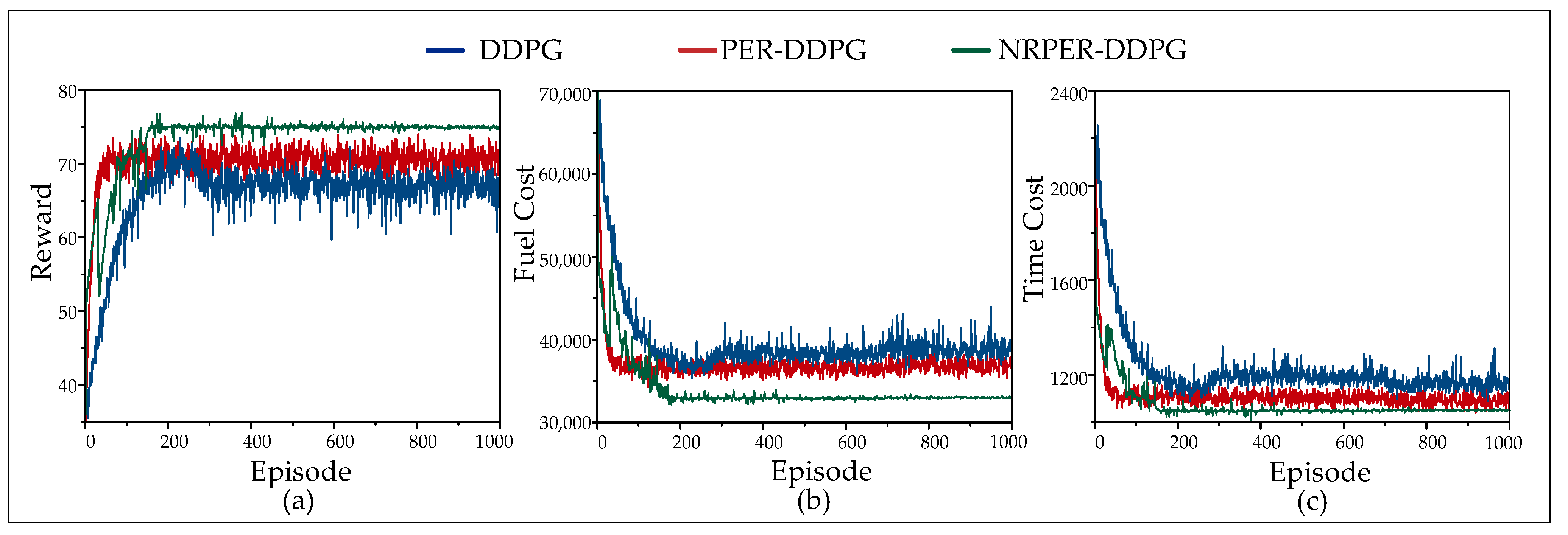
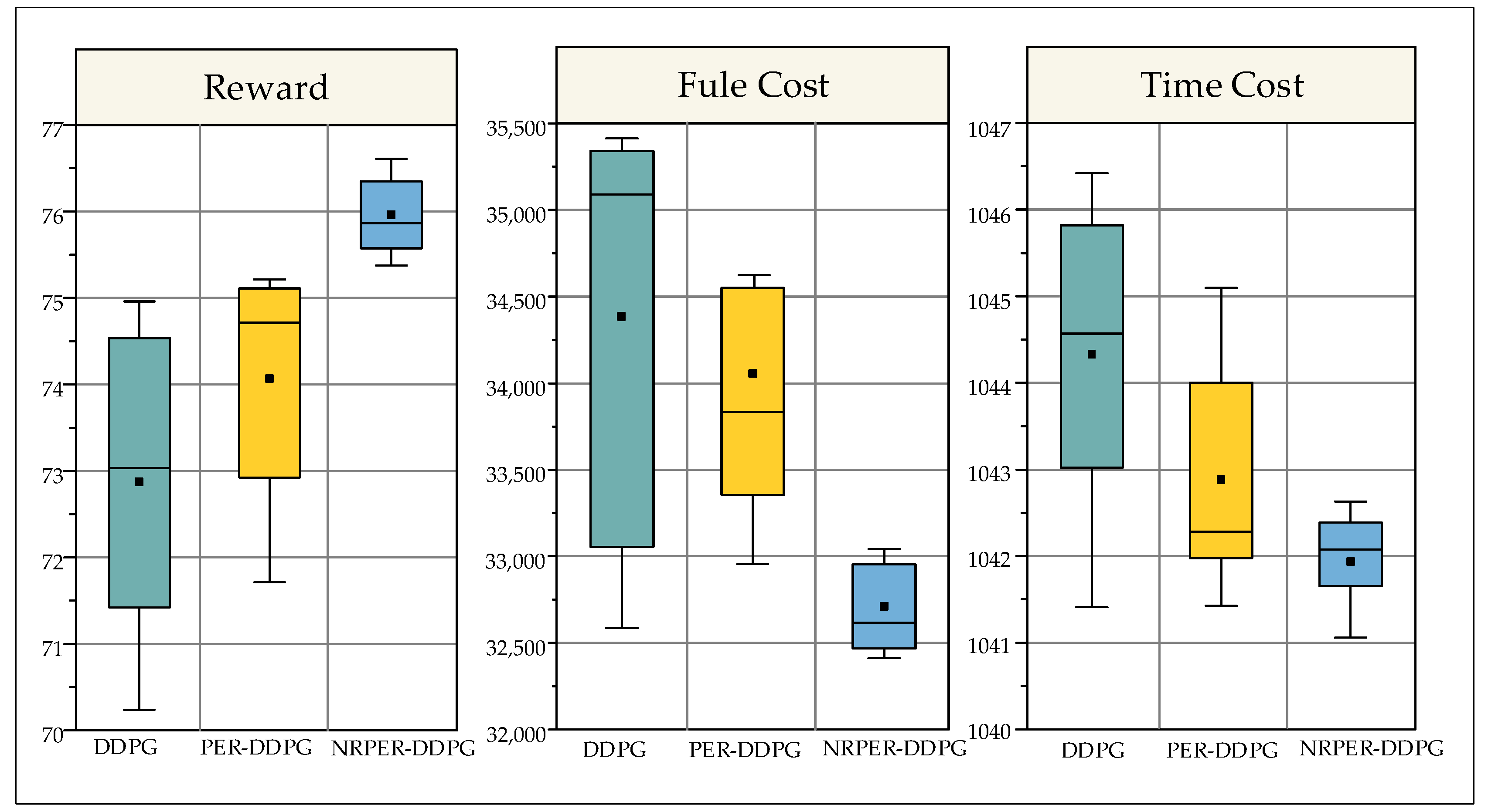
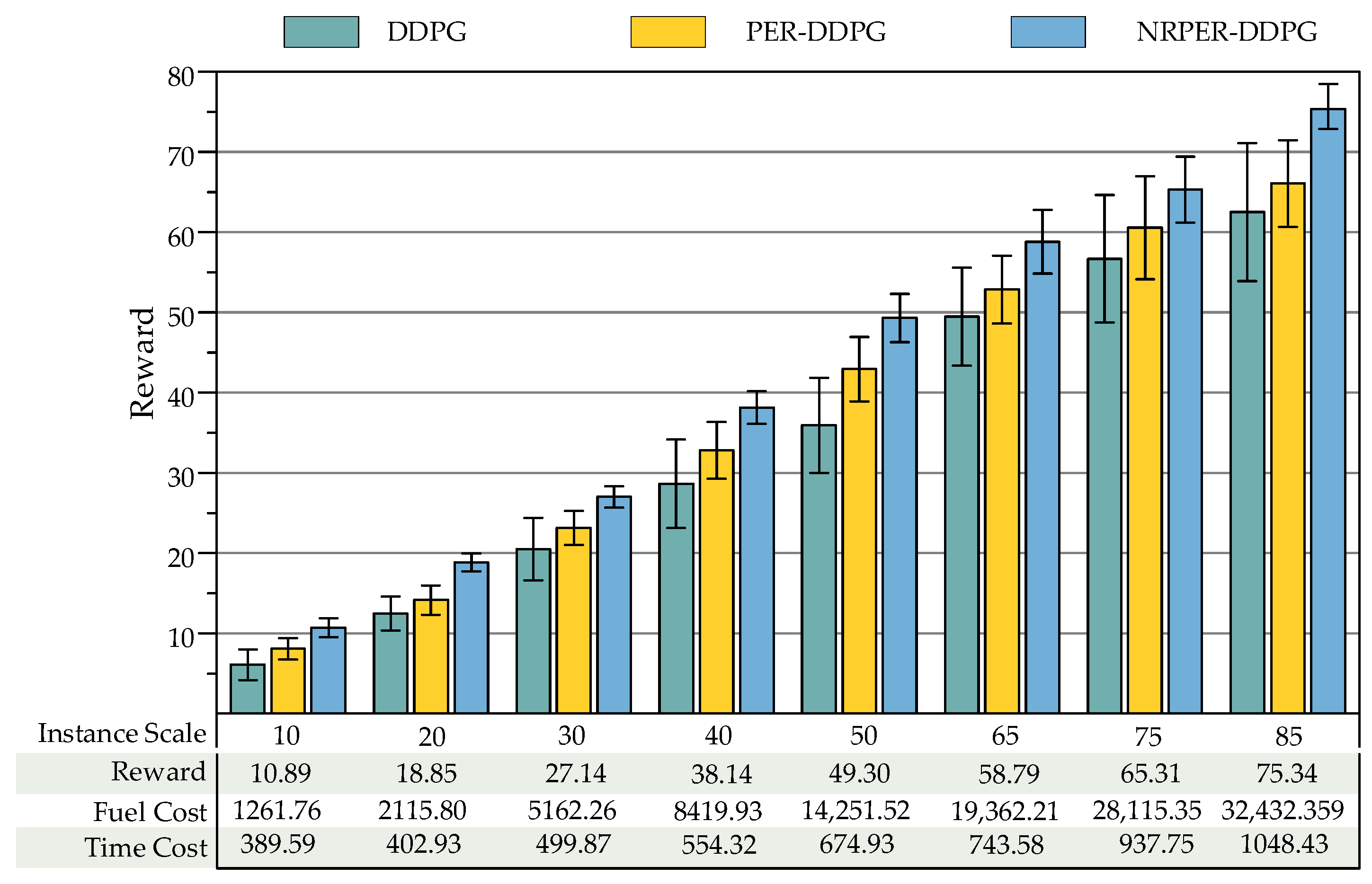
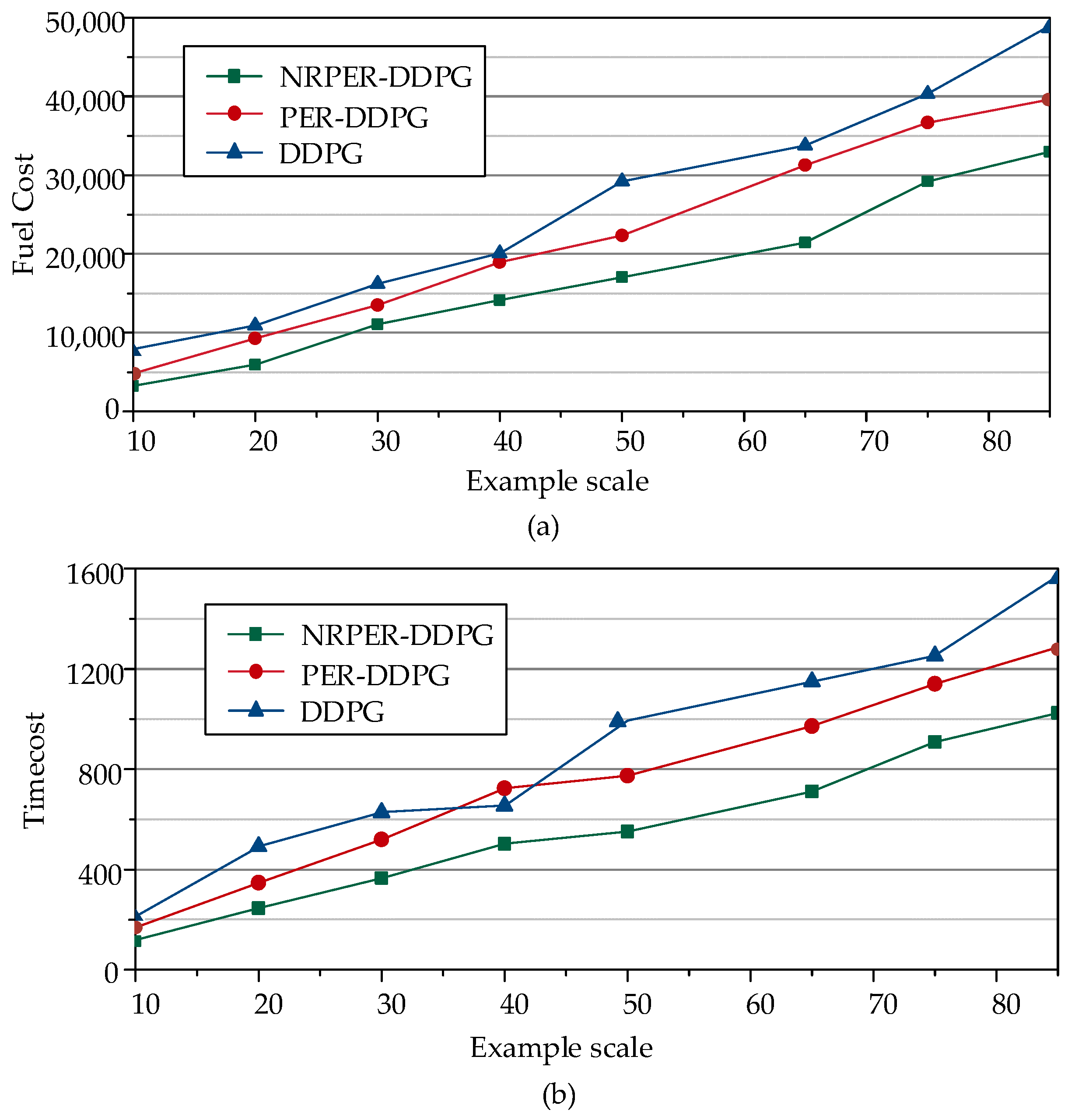
5.3. Simulation Case Study and Comparison
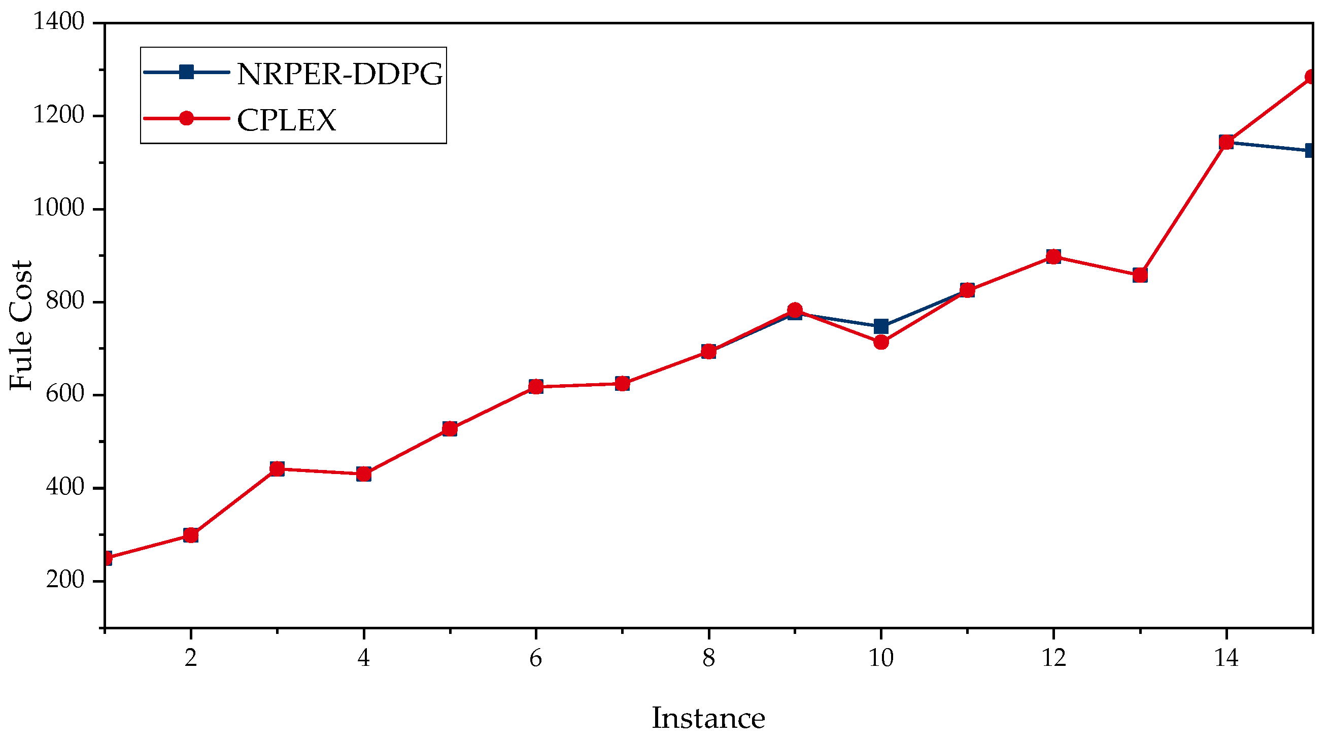
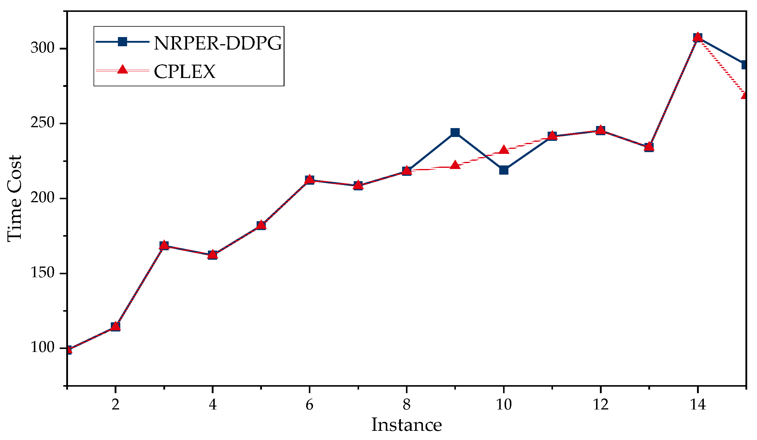
5.4. Experimental Comparison with CPLEX Solver
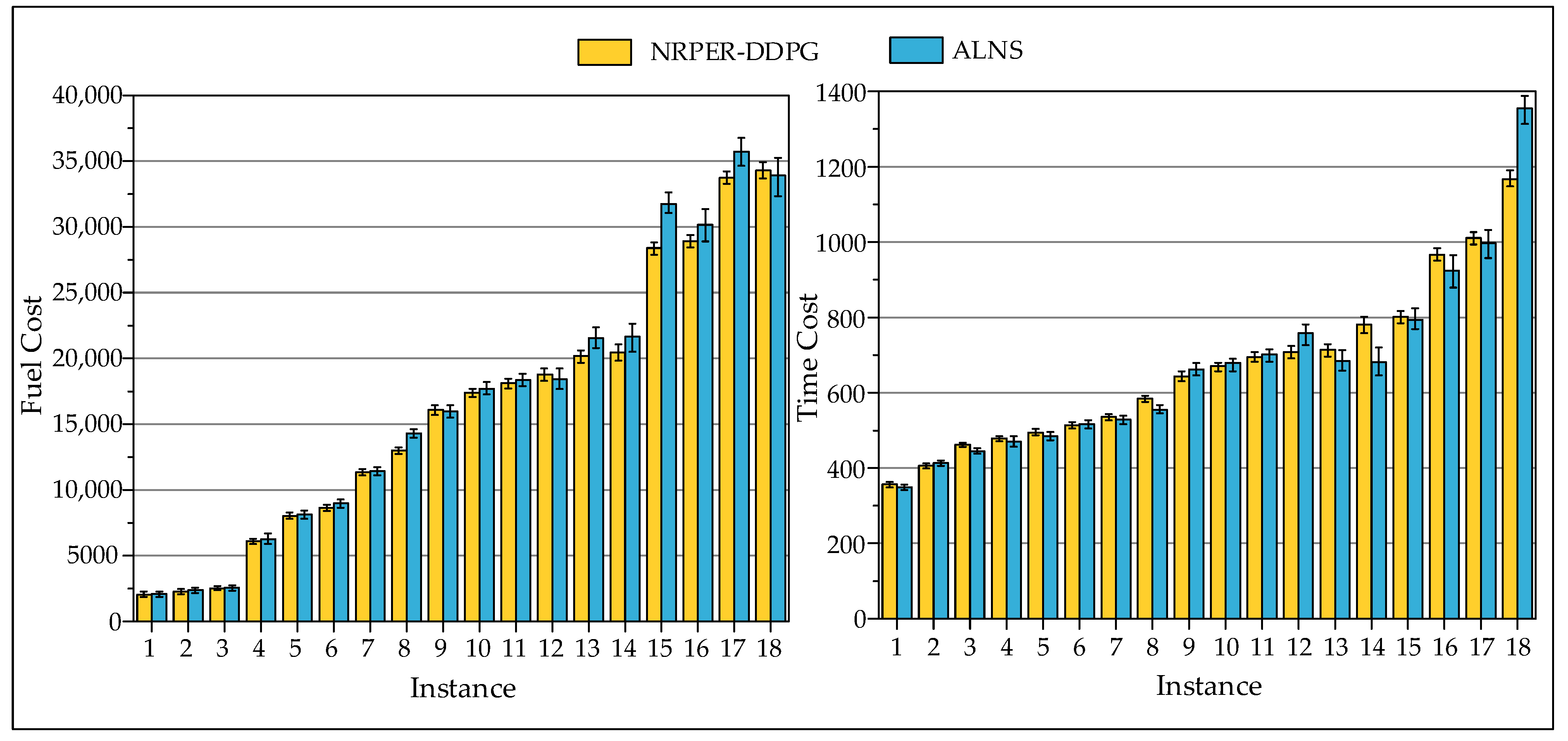
5.5. Conduct Comparative Experiments with the Existing Literature
5.6. Real-Case Experiment at Huanghua Port
6. Conclusions and Prospects
Author Contributions
Funding
Institutional Review Board Statement
Informed Consent Statement
Data Availability Statement
Conflicts of Interest
References
- Zhao, S.; Duan, J.; Li, D.; Yang, H. Vessel Scheduling and Bunker Management with Speed Deviations for Liner Shipping in the Presence of Collaborative Agreements. IEEE Access 2022, 10, 107669–107684. [Google Scholar] [CrossRef]
- Notteboom, T.E.; Vernimmen, B. The effect of high fuel costs on liner service configuration in container shipping. J. Transp. Geogr. 2008, 17, 325–337. [Google Scholar] [CrossRef]
- Wang, H.; Zhou, P.; Liang, Y.; Jeong, B.; Mesbahi, A. Optimization of tugboat propulsion system configurations: A holistic life cycle assessment case study. J. Clean. Prod. 2020, 259, 120903. [Google Scholar] [CrossRef]
- Zhu, J.; Chen, L.; Wang, B.; Xia, L. Optimal design of a hybrid electric propulsive system for an anchor handling tug supply vessel. Appl. Energy 2018, 226, 423–436. [Google Scholar] [CrossRef]
- Chen, Z.S.; Lam, J.S.L. Life cycle assessment of diesel and hydrogen power systems in tugboats. Transp. Res. Part D Transp. Environ. 2022, 103, 103192. [Google Scholar] [CrossRef]
- Liu, Z. Hybrid Evolutionary Strategy Optimization for Port Tugboat Operation Scheduling. In Proceedings of the 2009 Third International Symposium on Intelligent Information Technology Application, Nanchang, China, 21–22 November 2009; pp. 511–515. [Google Scholar] [CrossRef]
- Wang, S.; Kaku, I.; Chen, G.Y.; Zhu, M. Research on the modeling of tugboat assignment problem in container terminal. Adv. Mater. Res. 2012, 433, 1957–1961. [Google Scholar] [CrossRef]
- Ilati, G.; Sheikholeslami, A.; Hassannayebi, E. A Simulation-based optimization approach for integrated port resource allocation problem. PROMET-Traffic Transp. 2014, 26, 243–255. [Google Scholar] [CrossRef]
- Yang, Z.-Y.; Cao, X.; Xu, R.-Z.; Hong, W.-C.; Sun, S.-L. Applications of chaotic quantum adaptive satin bower bird optimizer algorithm in berth-tugboat-quay crane allocation optimization. Expert Syst. Appl. 2024, 237, 121471. [Google Scholar] [CrossRef]
- Wang, X.; Liang, Y.; Wei, X.; Chew, E.P. An adaptive large neighborhood search algorithm for the tugboat scheduling problem. Comput. Ind. Eng. 2023, 177, 109039. [Google Scholar] [CrossRef]
- Zhong, H.; Zhang, Y.; Gu, Y. A Bi-objective green tugboat scheduling problem with the tidal port time windows. Transp. Res. Part D Transp. Environ. 2022, 110, 103409. [Google Scholar] [CrossRef]
- Wei, X.; Jia, S.; Meng, Q.; Tan, K.C. Tugboat scheduling for container ports. Transp. Res. Part E Logist. Transp. Rev. 2020, 142, 102071. [Google Scholar] [CrossRef]
- Kasm, O.A.; Diabat, A.; Ozbay, K. Vessel scheduling under different tugboat allocation policies. Comput. Ind. Eng. 2023, 177, 108902. [Google Scholar] [CrossRef]
- Kang, L.; Meng, Q.; Tan, K.C. Tugboat scheduling under ship arrival and tugging process time uncertainty. Transp. Res. Part E Logist. Transp. Rev. 2020, 144, 102125. [Google Scholar] [CrossRef]
- Hao, L.; Jin, J.G.; Zhao, K. Joint scheduling of barges and tugboats for river–sea intermodal transport. Transp. Res. Part E Logist. Transp. Rev. 2023, 173, 103097. [Google Scholar] [CrossRef]
- Jia, S.; Li, S.; Lin, X.; Chen, X. Scheduling tugboats in a seaport. Transp. Sci. 2021, 55, 1370–1391. [Google Scholar] [CrossRef]
- Morariu, C.; Morariu, O.; Răileanu, S.; Borangiu, T. Machine learning for predictive scheduling and resource allocation in large scale manufacturing systems. Comput. Ind. 2020, 120, 103244. [Google Scholar] [CrossRef]
- Liu, Z.; Wang, Y.; Liang, X.; Ma, Y.; Feng, Y.; Cheng, G.; Liu, Z. A graph neural networks-based deep Q-learning approach for job shop scheduling problems in traffic management. Inf. Sci. 2022, 607, 1211–1223. [Google Scholar] [CrossRef]
- Zonta, T.; da Costa, C.A.; Zeiser, F.A.; Ramos, G.d.O.; Kunst, R.; Righi, R.d.R. A predictive maintenance model for optimizing production schedule using deep neural networks. J. Manuf. Syst. 2022, 62, 450–462. [Google Scholar] [CrossRef]
- Wang, L.; Pan, Z.; Wang, J. A review of reinforcement learning based intelligent optimization for manufacturing scheduling. Complex Syst. Model. Simul. 2021, 1, 257–270. [Google Scholar] [CrossRef]
- Liu, R.; Piplani, R.; Toro, C. A deep multi-agent reinforcement learning approach to solve dynamic job shop scheduling problem. Comput. Oper. Res. 2023, 159, 106294. [Google Scholar] [CrossRef]
- Zou, Y.; Yin, H.; Zheng, Y.; Dressler, F. Multi-agent reinforcement learning enabled link scheduling for next generation Internet of Things. Comput. Commun. 2023, 205, 35–44. [Google Scholar] [CrossRef]
- Ziaei, F.; Ranjbar, M. A reinforcement learning algorithm for scheduling parallel processors with identical speedup functions. Mach. Learn. Appl. 2023, 13, 100485. [Google Scholar] [CrossRef]
- Zhang, N.; Shen, Y.; Du, Y.; Chen, L.; Zhang, X. Counterfactual-attention multi-agent reinforcement learning for joint condition-based maintenance and production scheduling. J. Manuf. Syst. 2023, 71, 70–81. [Google Scholar] [CrossRef]
- Li, R.; Zhang, X.; Jiang, L.; Yang, Z.; Guo, W. An adaptive heuristic algorithm based on reinforcement learning for ship scheduling optimization problem. Ocean Coast. Manag. 2022, 230, 106375. [Google Scholar] [CrossRef]
- Drungilas, D.; Kurmis, M.; Senulis, A.; Lukosius, Z.; Andziulis, A.; Januteniene, J.; Bogdevicius, M.; Jankunas, V.; Voznak, M. Deep reinforcement learning based optimization of automated guided vehicle time and energy consumption in a container terminal. Alex. Eng. J. 2023, 67, 397–407. [Google Scholar] [CrossRef]
- Chen, X.; Liu, S.; Zhao, J.; Wu, H.; Xian, J.; Montewka, J. Autonomous port management based AGV path planning and optimization via an ensemble reinforcement learning framework. Ocean Coast. Manag. 2024, 251, 107087. [Google Scholar] [CrossRef]
- Jin, J.; Cui, T.; Bai, R.; Qu, R. Container port truck dispatching optimization using Real2Sim based deep reinforcement learning. Eur. J. Oper. Res. 2024, 315, 161–175. [Google Scholar] [CrossRef]
- Tofighi, S.; Torabi, S.; Mansouri, S. Humanitarian logistics network design under mixed uncertainty. Eur. J. Oper. Res. 2016, 250, 239–250. [Google Scholar] [CrossRef]
- Zheng, X.; Liang, C.; Wang, Y.; Shi, J.; Lim, G. Multi-AGV Dynamic Scheduling in an Automated Container Terminal: A Deep Reinforcement Learning Approach. Mathematics 2022, 10, 4575. [Google Scholar] [CrossRef]
- Bachiri, K.; Yahyaouy, A.; Gualous, H.; Malek, M.; Bennani, Y.; Makany, P.; Rogovschi, N. Multi-Agent DDPG Based Electric Vehicles Charging Station Recommendation. Energies 2023, 16, 6067. [Google Scholar] [CrossRef]
- Jiang, X.; Zhong, M.; Shi, G.; Li, W.; Sui, Y. Vessel scheduling model with resource restriction considerations for restricted channel in ports. Comput. Ind. Eng. 2023, 177, 109034. [Google Scholar] [CrossRef]
- Sha, Z.; Huo, R.; Sun, C.; Wang, S.; Huang, T. A Task-Oriented Hybrid Routing Approach based on Deep Deterministic Policy Gradient. Comput. Commun. 2023, 210, 183–193. [Google Scholar] [CrossRef]
- Liu, Y.; Liang, H.; Xiao, Y.; Zhang, H.; Zhang, J.; Zhang, L.; Wang, L. Logistics-involved service composition in a dynamic cloud manufacturing environment: A DDPG-based approach. Robot. Comput.-Integr. Manuf. 2022, 76, 102323. [Google Scholar] [CrossRef]
- Liu, G.; Chen, G.; Huang, V. Policy ensemble gradient for continuous control problems in deep reinforcement learning. Neurocomputing 2023, 548, 126381. [Google Scholar] [CrossRef]
- Park, H.; Choi, D.G.; Min, D. Adaptive inventory replenishment using structured reinforcement learning by exploiting a policy structure. Int. J. Prod. Econ. 2023, 266, 109029. [Google Scholar] [CrossRef]
- Zhu, M.; Tian, K.; Wen, Y.Q.; Cao, J.N.; Huang, L. Improved PER-DDPG based nonparametric modeling of ship dynamics with uncertainty. Ocean. Eng. 2023, 286 Pt 1, 115513. [Google Scholar] [CrossRef]
- Cai, Z.; Lee, F.; Hu, C.; Kotani, K.; Chen, Q. NAEM: Noisy Attention Exploration Module for Deep Reinforcement Learning. IEEE Access 2021, 9, 154600–154611. [Google Scholar] [CrossRef]
- Han, S.; Zhou, W.B.; Lu, J.Y.; Liu, J.; Lü, S. NROWAN-DQN: A stable noisy network with noise reduction and online weight adjustment for exploration. Expert Syst. Appl. 2022, 203, 117343. [Google Scholar] [CrossRef]
- Ministry of Transportation and Communications. Circular of the National Development and Reform Commission on the Revision and Issuance of the Measures for the Billing of Port Charges; Ministry of Transportation and Communications: Beijing, China, 2019.


| Parameter Type | Parameter | Description |
|---|---|---|
| Set | i | Tugboat number, |
| j | Task number, | |
| k | Base number, | |
| The distance from tugboat i at base k to the starting point of task j | ||
| Distance from tug i at base k to the ending point of task j | ||
| The fuel cost per unit time of tugboat i during navigation assistance | ||
| The fuel cost per unit distance for tugboat i when it is unloaded (or empty) | ||
| Input Parameters | The power required for the tugboats assigned to task j | |
| The number of tugboats required for task j | ||
| The power of tugboat i | ||
| Tugboat i is at base k after completing the previous task | ||
| Time of arrival of vessel for task j at the starting point | ||
| Time of arrival of vessel for task j at the ending point | ||
| The speed of tugboat i when it is unloaded (or empty) | ||
| The time window for the tugboats to arrive at the starting point of the task | ||
| The return time window for tugboats upon task completion. | ||
| Output Parameters | Total fuel cost incurred by the tugboats | |
| Total waiting time cost incurred by the vessels awaiting operation | ||
| Decision variables | If tugboat i is assigned to task j, the value is 1; otherwise 0 | |
| If tugboat i is at base k after task j, the value is 1; otherwise 0 |
| Parameters | Value | Parameters | Value |
|---|---|---|---|
| Uniform [1, 4] | Task generation probability | 0.4 | |
| (n mile) | Uniform [10, 20] | Learning rate lr | |
| (n mile) | Uniform [10, 20] | Reward discount factor γ | 0.1 |
| (USD) | Uniform [8, 12] | Soft update coefficient ξ | 0.01 |
| (USD) | Uniform [20, 28] | Maximum number of episodes Itmax | 1000 |
| (hp) | Uniform [3000, 6000] | Target network parameter update frequency | 100 |
| (hp) | Uniform [3000, 6000] | Experience replay buffer capacity R | |
| (n mile/h) | Uniform [6, 15] | Batch size N | 64 |
| η | Reward | Fuel Cost (USD) | Time Cost (min) |
|---|---|---|---|
| 0.2 | 33.8847 | 288,830.9563 | 683.5225 |
| 0.4 | 34.6327 | 282,682.3915 | 652.3833 |
| 0.6 | 33.2221 | 296,113.7766 | 706.1413 |
| 0.8 | -- | -- | -- |
| Numerical Example | Vessel | Tugboat | Tugboat Base |
|---|---|---|---|
| 1 | 10 | 16 | 6 |
| 2 | 20 | 32 | 12 |
| 3 | 30 | 48 | 18 |
| 4 | 40 | 64 | 24 |
| 5 | 50 | 80 | 30 |
| 6 | 65 | 104 | 39 |
| 7 | 75 | 112 | 45 |
| 8 | 85 | 120 | 51 |
| ID | I | J | K | NRPER-DDPG | CPLEX | ||||
|---|---|---|---|---|---|---|---|---|---|
| Fuel Cost | Time Cost | CPU Time | Fuel Cost | Time Cost | CPU Time | ||||
| 1 | 5 | 5 | 3 | 249.62 | 98.87 | 2.52 | 249.62 | 98.87 | 0.34 |
| 2 | 5 | 6 | 4 | 298.81 | 114.24 | 2.63 | 298.81 | 114.24 | 0.29 |
| 3 | 5 | 7 | 5 | 441.13 | 168.36 | 2.68 | 441.13 | 168.36 | 0.36 |
| 4 | 7 | 7 | 5 | 430.40 | 162.14 | 2.74 | 430.40 | 162.14 | 0.58 |
| 5 | 7 | 8 | 6 | 527.58 | 181.89 | 2.73 | 527.58 | 181.89 | 1.73 |
| 6 | 7 | 9 | 7 | 618.23 | 212.23 | 2.77 | 618.23 | 212.23 | 3.69 |
| 7 | 9 | 9 | 6 | 624.85 | 208.36 | 2.89 | 624.85 | 208.36 | 5.80 |
| 8 | 9 | 10 | 7 | 693.46 | 218.07 | 2.62 | 693.46 | 218.07 | 12.84 |
| 9 | 9 | 11 | 8 | 775.91 | 243.94 | 3.04 | 782.73 | 221.67 | 33.47 |
| 10 | 11 | 11 | 7 | 747.15 | 218.93 | 3.15 | 713.26 | 231.94 | 58.62 |
| 11 | 11 | 12 | 8 | 825.41 | 241.34 | 3.22 | 825.41 | 241.34 | 113.71 |
| 12 | 11 | 13 | 9 | 897.36 | 245.16 | 3.35 | 897.36 | 245.16 | 158.79 |
| 13 | 13 | 13 | 8 | 857.94 | 233.98 | 3.37 | 857.94 | 233.98 | 367.60 |
| 14 | 13 | 14 | 9 | 1069.70 | 287.52 | 3.40 | -- | -- | 2000 |
| 15 | 13 | 15 | 10 | 1143.87 | 307.12 | 3.64 | 1143.87 | 307.12 | 875.91 |
| 16 | 15 | 15 | 9 | 1125.72 | 289.23 | 3.72 | 1284.62 | 268.35 | 1374.25 |
| 17 | 15 | 16 | 10 | 1205.43 | 308.10 | 4.86 | -- | -- | 2000 |
| 18 | 15 | 17 | 11 | 1267.51 | 319.79 | 6.88 | -- | -- | 2000 |
| ID | I | J | K | NRPER-DDPG (10 runs) | ALNS [10] (10 runs) | ||||
|---|---|---|---|---|---|---|---|---|---|
| Fuel Cost | Time Cost | CPU Time | Fuel Cost | Time Cost | CPU Time | ||||
| 1 | 30 | 20 | 12 | 2044.04 | 357.18 | 10.21 | 2087.13 | 349.18 | 7.46 |
| 2 | 40 | 22 | 15 | 2265.39 | 406.16 | 10.32 | 2379.26 | 413.57 | 14.51 |
| 3 | 45 | 28 | 18 | 2518.23 | 462.15 | 22.97 | 2562.57 | 445.30 | 19.68 |
| 4 | 55 | 30 | 22 | 6111.06 | 478.71 | 24.16 | 6254.71 | 470.19 | 33.62 |
| 5 | 65 | 32 | 25 | 8016.29 | 494.35 | 35.80 | 8114.63 | 484.31 | 42.59 |
| 6 | 70 | 36 | 28 | 8644.38 | 513.73 | 47.89 | 8982.86 | 517.22 | 60.68 |
| 7 | 75 | 44 | 31 | 11,330.87 | 536.02 | 61.26 | 11,426.92 | 528.61 | 88.20 |
| 8 | 80 | 46 | 34 | 13,008.06 | 584.22 | 84.19 | 14,295.65 | 554.37 | 102.69 |
| 9 | 85 | 52 | 37 | 16,081.48 | 643.65 | 116.12 | 15,973.71 | 662.11 | 166.25 |
| 10 | 90 | 54 | 40 | 17,402.96 | 671.08 | 252.68 | 17,681.45 | 679.48 | 274.91 |
| 11 | 95 | 60 | 43 | 18,120.26 | 695.48 | 314.09 | 18,355.94 | 701.38 | 368.35 |
| 12 | 100 | 62 | 46 | 18,768.37 | 707.83 | 435.15 | 18,406.62 | 758.97 | 487.24 |
| 13 | 105 | 68 | 49 | 20,206.46 | 714.16 | 497.07 | 21,564.17 | 684.34 | 531.54 |
| 14 | 110 | 70 | 52 | 20,443.59 | 781.52 | 625.98 | 21,648.43 | 681.16 | 753.80 |
| 15 | 115 | 86 | 55 | 28,397.06 | 801.51 | 726.09 | 31,751.16 | 793.50 | 813.44 |
| 16 | 120 | 88 | 58 | 28,909.40 | 966.10 | 810.80 | 30,149.57 | 924.28 | 1348.21 |
| 17 | 125 | 94 | 61 | 33,723.62 | 1011.44 | 872.15 | 35,729.83 | 997.55 | 1815.57 |
| 18 | 130 | 96 | 64 | 34,294.32 | 1167.19 | 938.56 | 33,915.36 | 1354.70 | 1893.26 |
| Task | Required Number of Tugboats | Required Tugboat Power (hp) | Berthing or Departure | Task Start Time |
|---|---|---|---|---|
| 1 | 2 | 2000 | Departure | 0:00 |
| 2 | 2 | 2000 | Berthing | 2:30 |
| 3 | 2 | 3000 | Berthing | 5:00 |
| 4 | 3 | 3000 | Departure | 9:00 |
| 5 | 2 | 2000 | Berthing | 10:00 |
| 6 | 2 | 3000 | Departure | 12:00 |
| 7 | 3 | 5000 | Departure | 12:00 |
| 8 | 2 | 4000 | Berthing | 13:30 |
| 9 | 2 | 2000 | Berthing | 14:30 |
| 10 | 2 | 2000 | Berthing | 16:00 |
| 11 | 3 | 3000 | Departure | 18:00 |
| 12 | 2 | 2000 | Departure | 21:00 |
| 13 | 5 | 5000 | Berthing | 21:00 |
| 14 | 3 | 4000 | Departure | 22:00 |
| 15 | 3 | 3000 | Departure | 23:00 |
| Method | Fuel Cost (USD) | Time Cost (min) |
|---|---|---|
| CPLEX | 8774.62 | 1088.32 |
| ALNS | 9137.81 | 974.25 |
| NRPER-DDPG | 8774.62 | 1088.32 |
Disclaimer/Publisher’s Note: The statements, opinions and data contained in all publications are solely those of the individual author(s) and contributor(s) and not of MDPI and/or the editor(s). MDPI and/or the editor(s) disclaim responsibility for any injury to people or property resulting from any ideas, methods, instructions or products referred to in the content. |
© 2024 by the authors. Licensee MDPI, Basel, Switzerland. This article is an open access article distributed under the terms and conditions of the Creative Commons Attribution (CC BY) license (https://creativecommons.org/licenses/by/4.0/).
Share and Cite
Li, J.; Duan, X.; Xiong, Z.; Yao, P. Tugboat Scheduling Method Based on the NRPER-DDPG Algorithm: An Integrated DDPG Algorithm with Prioritized Experience Replay and Noise Reduction. Sustainability 2024, 16, 3379. https://doi.org/10.3390/su16083379
Li J, Duan X, Xiong Z, Yao P. Tugboat Scheduling Method Based on the NRPER-DDPG Algorithm: An Integrated DDPG Algorithm with Prioritized Experience Replay and Noise Reduction. Sustainability. 2024; 16(8):3379. https://doi.org/10.3390/su16083379
Chicago/Turabian StyleLi, Jiachen, Xingfeng Duan, Zhennan Xiong, and Peng Yao. 2024. "Tugboat Scheduling Method Based on the NRPER-DDPG Algorithm: An Integrated DDPG Algorithm with Prioritized Experience Replay and Noise Reduction" Sustainability 16, no. 8: 3379. https://doi.org/10.3390/su16083379
APA StyleLi, J., Duan, X., Xiong, Z., & Yao, P. (2024). Tugboat Scheduling Method Based on the NRPER-DDPG Algorithm: An Integrated DDPG Algorithm with Prioritized Experience Replay and Noise Reduction. Sustainability, 16(8), 3379. https://doi.org/10.3390/su16083379