
Satisfaction-Based Optimal Lane Change Modelling of Mixed Traffic Flow and Intersection Vehicle Guidance Control Method in an Intelligent and Connected Environment

Abstract
:1. Introduction
2. Modelling of Mixed Traffic Flow Lane-Changing Based on Global Priority Capacity
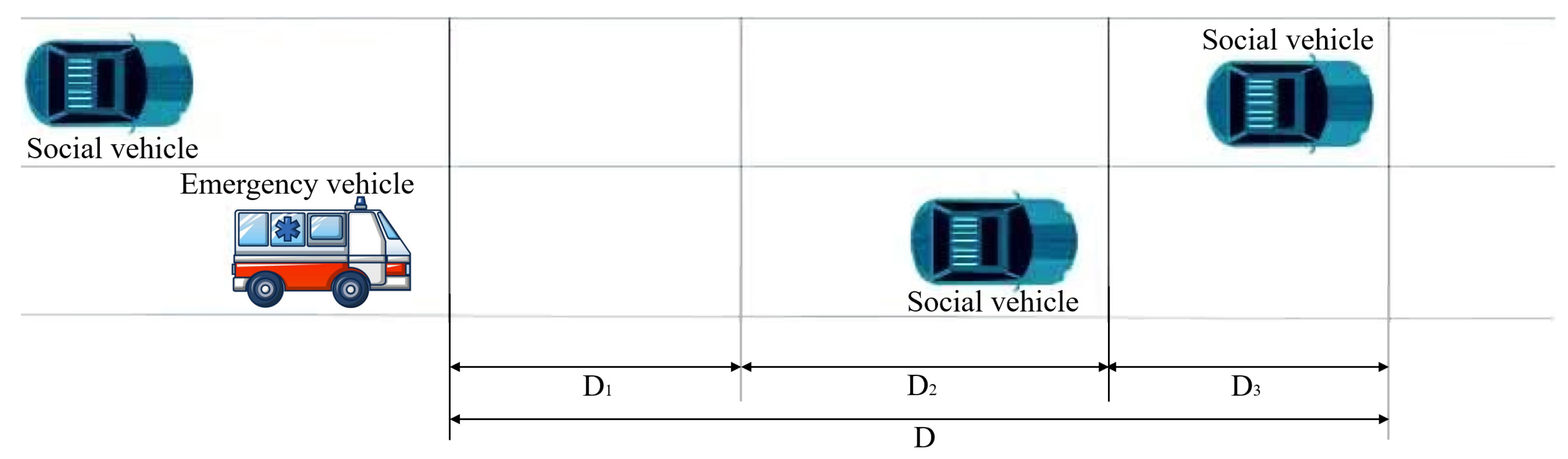
2.1. Scenario Description
2.2. A Study of Lane-Changing Modelling
2.2.1. Construction of Mixed Traffic Flow Lane-Changing Model Based on Driver Satisfaction
2.2.2. Construction of the Social Vehicle Lane-Change Type Based on the Influence Characteristics of Emergency Vehicles
2.3. Vehicle-Following Lane-Changing Model Implementation
3. An Active Guidance Method for Mixed Traffic Flow
3.1. The Theoretical Foundation for Speed Guidance
- (1)
- Optimal velocity model (OV) model
- (2)
- Generalized Force (GF) model
3.2. A Mixed Traffic Flow Guidance Scenario Analysis
- In a connected vehicle with optimal communication conditions, each vehicle is able to communicate with other vehicles and roadside equipment units. Furthermore, the connected vehicles are capable of cooperative control, enabling them to complete assigned driving tasks as directed by the control centre.
- The communication between the vehicle-mounted equipment of the connected vehicles and the roadside equipment is facilitated by a special vehicle networking communication protocol (IEEE 802.11p protocol), which ensures the accuracy and real-time nature of the collected information.
- The influence of external factors, such as non-motorized vehicles and pedestrians, is disregarded.
- The vehicles within the control area are operating in accordance with the relevant regulations.
- All vehicles are travelling at the same desired speed.
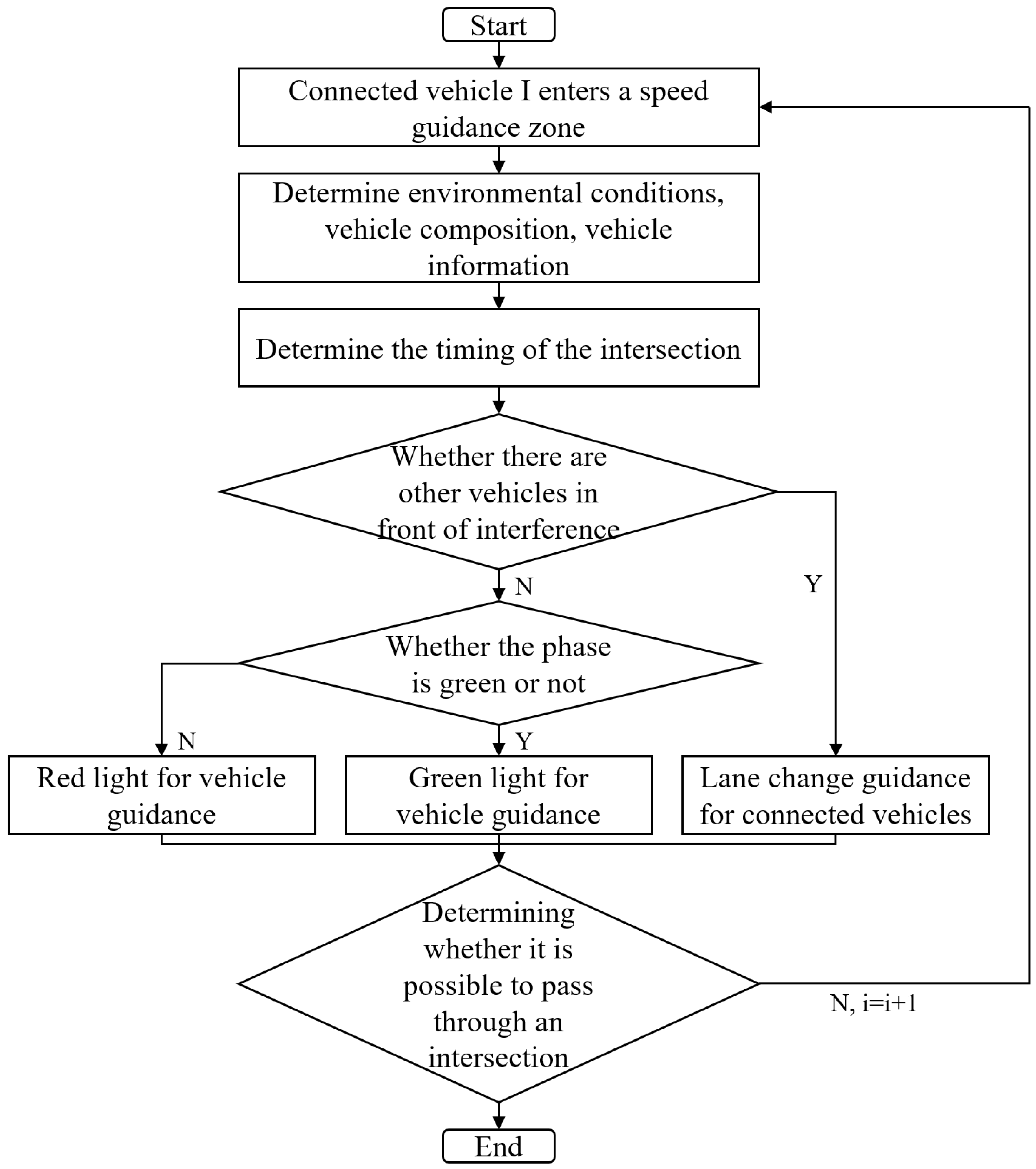
3.3. Methodology
- (1)
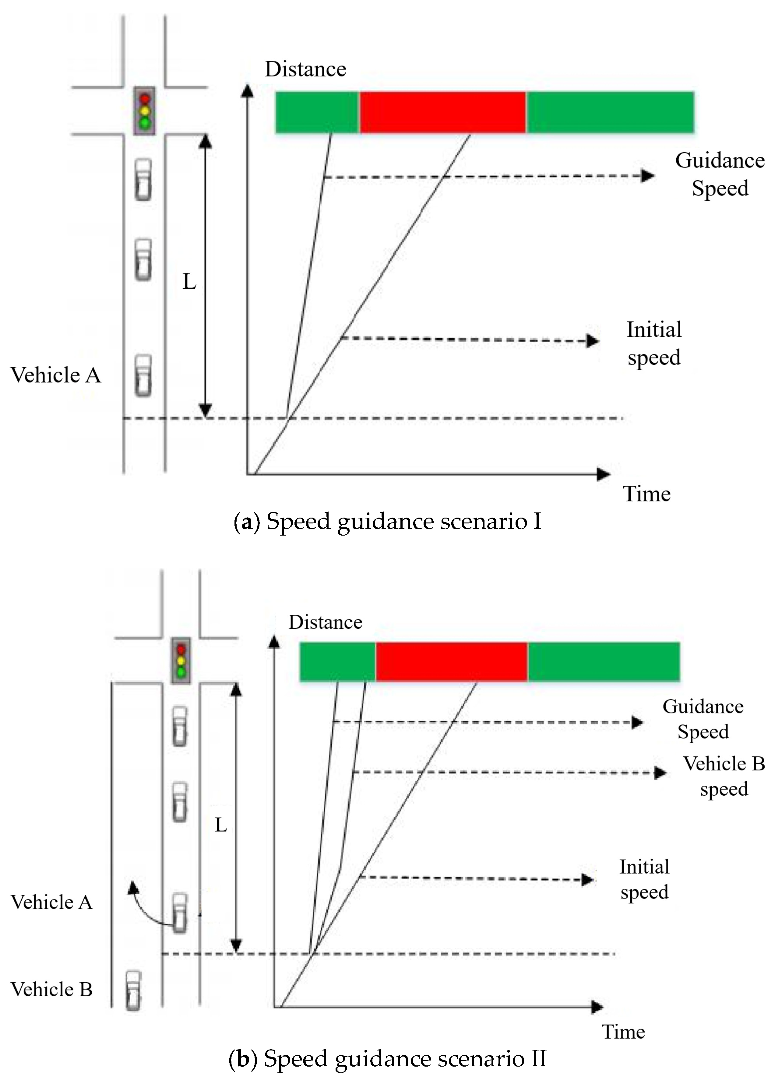
- In the event of the light = G, the vehicle enters the speed guidance zone and the intersection signal is green. Despite the optimal guidance speed of vehicle A being calculated, it is possible for it to pass in the green light time, as illustrated in Figure 4a. The presence of the vehicle in front of it constitutes an obstacle, and it is not feasible to proceed according to the guidance speed in order to avoid a potential conflict. Consequently, it is not possible to pass through the intersection within the allotted time frame for the green light.
- (2)
- When light = R, after entering the speed guidance area, the vehicle must adhere to the speed guidance Equation (37) in the event of a red-light phase, the presence of vehicles in front of an obstruction, or a queueing phenomenon, as illustrated in Figure 5.
- (1)
- In the case of light = G (see Figure 6a), upon entering the speed guidance zone, the intersection signal ahead is green and there are no queuing conditions. However, if vehicle A continues to enter the speed guidance zone at its initial speed v forward, it may encounter a red-light phase when reaching the intersection stop line. At this juncture, it is advisable to increase the speed of the vehicles to facilitate the passage of vehicle A through the intersection during the green light interval.
- (2)
- In the case of light = R (see Figure 6b), the vehicle enters the speed guidance zone with the intersection ahead displaying a red signal. In such instances, the initial speed v is adjusted to prevent the vehicle from reaching the intersection stop line during the red-light phase.
4. Case Study
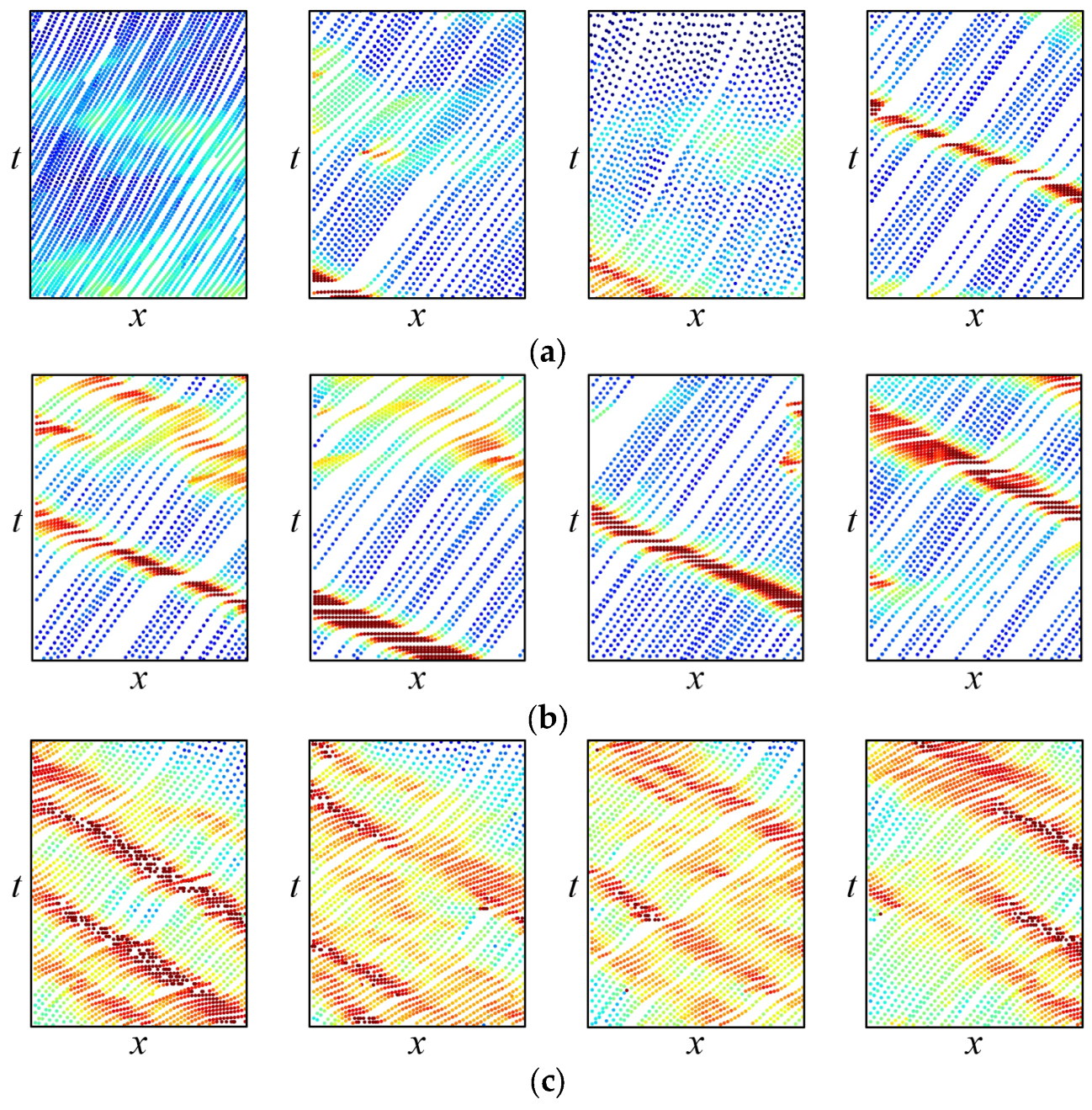
4.1. The Results of Mixed Traffic Flow Lane-Changing Model
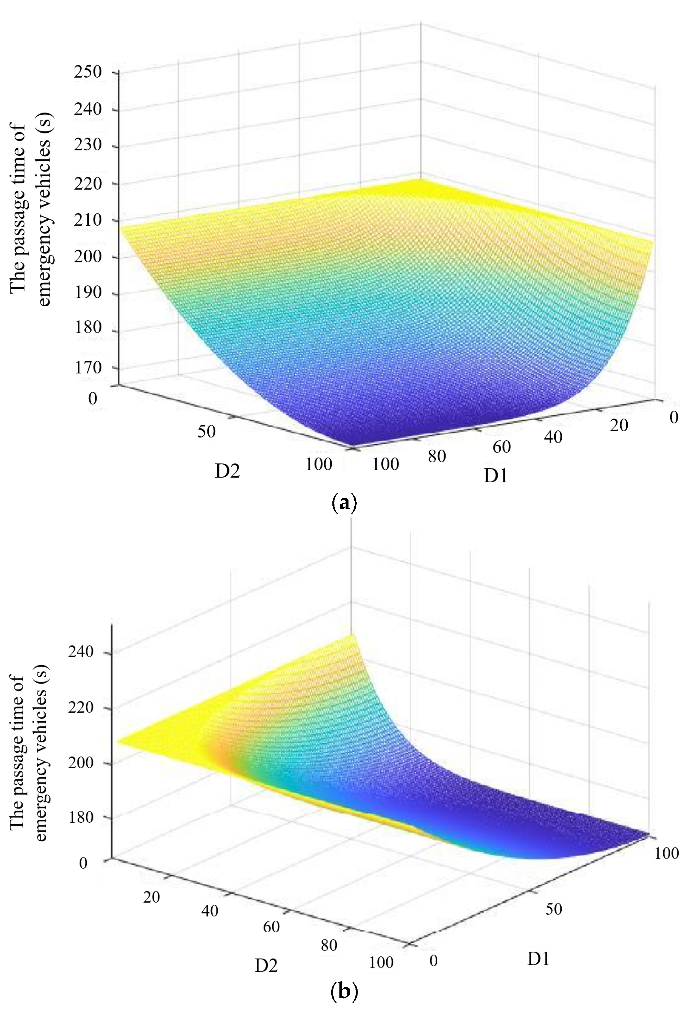
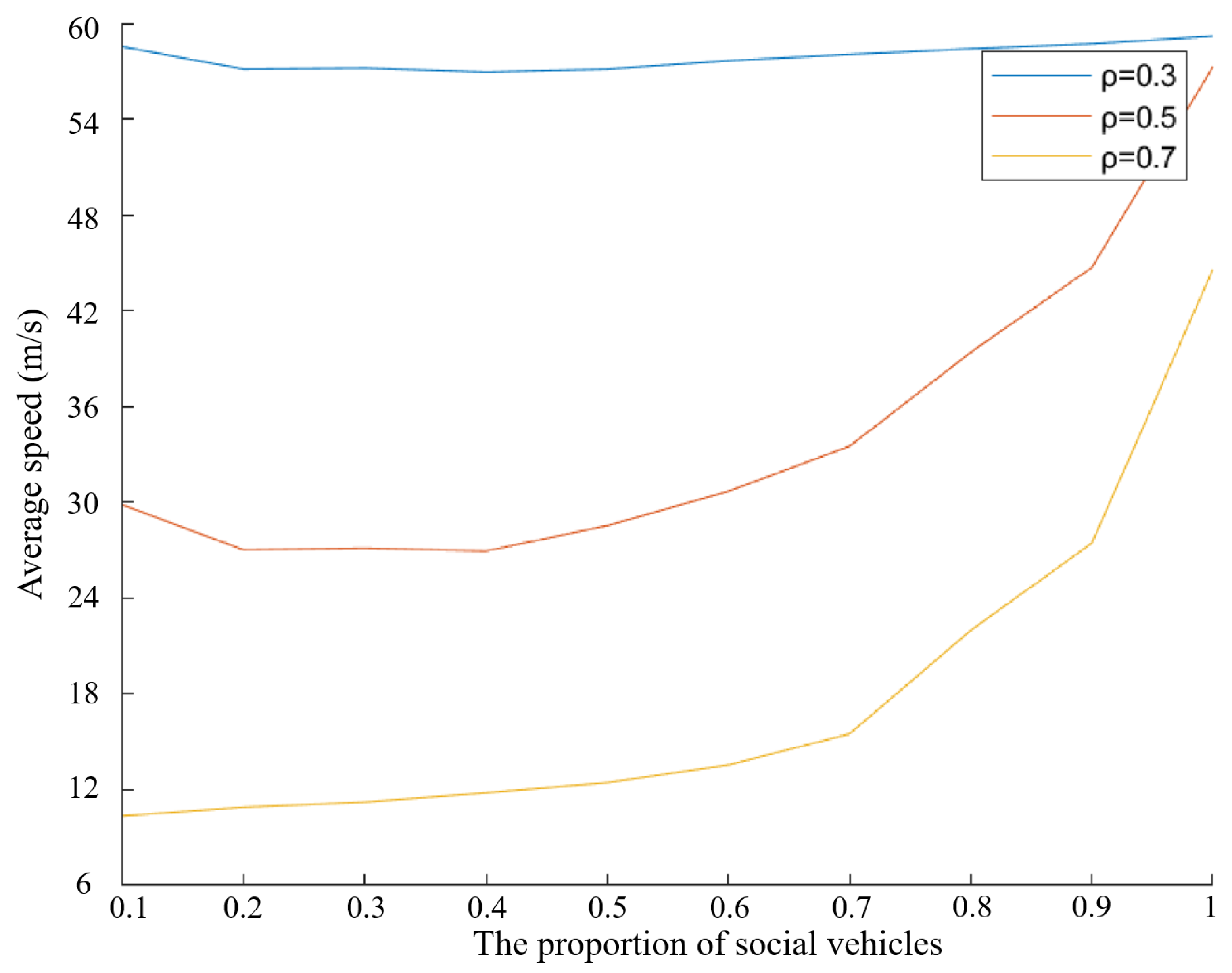
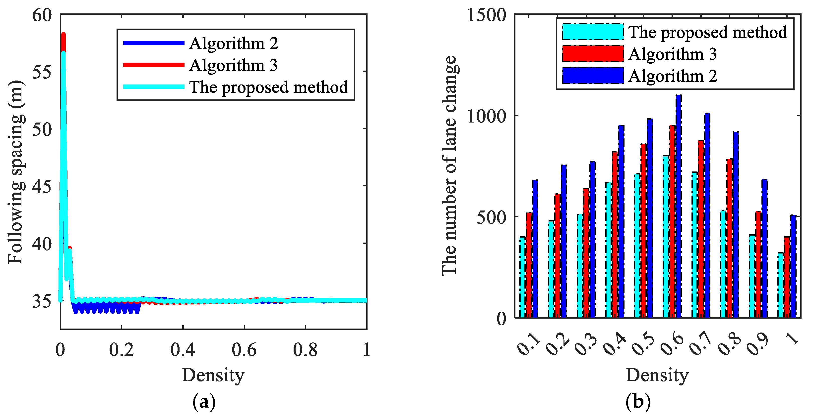
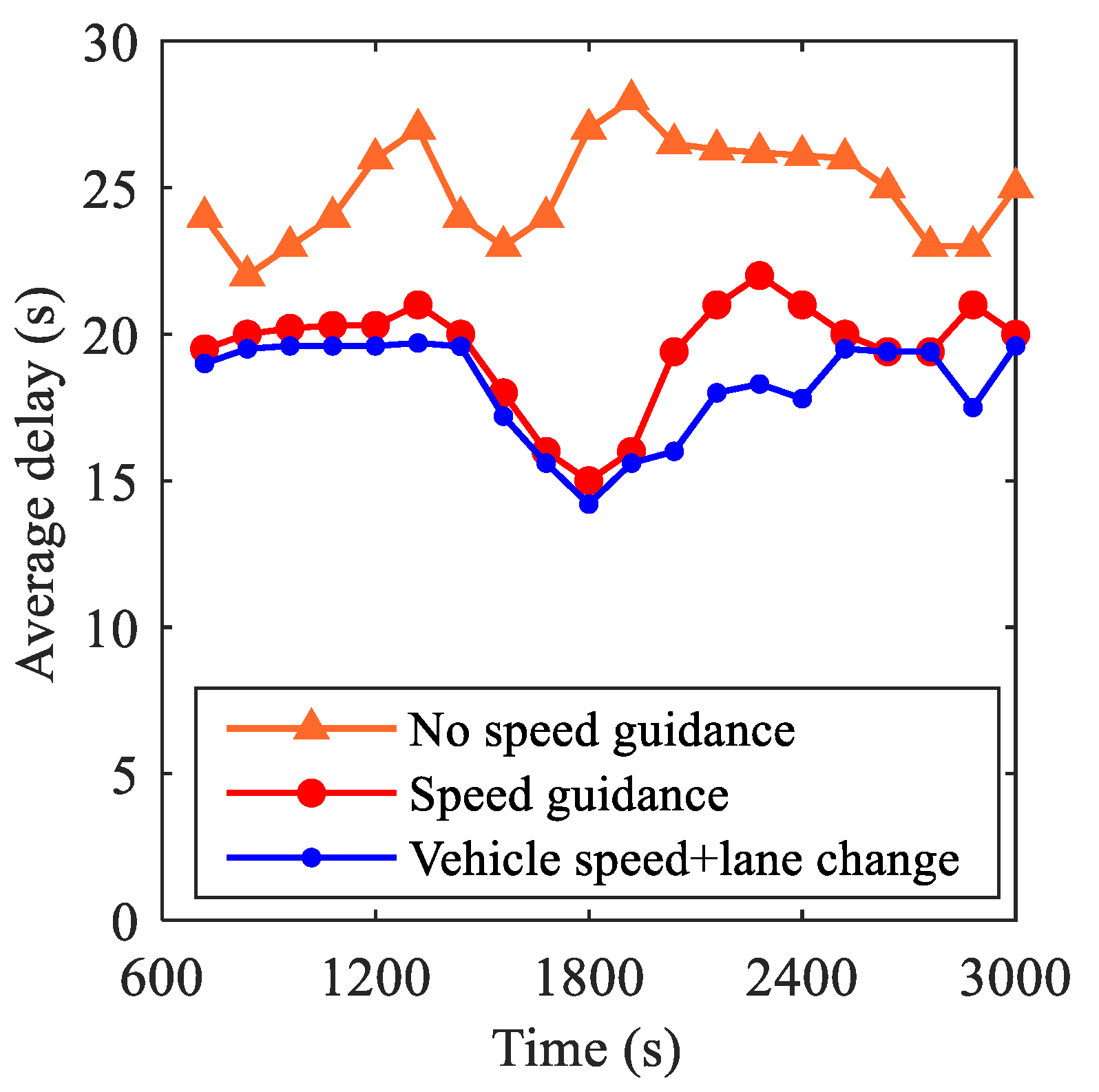
4.2. The Results of Active Guidance for Mixed Traffic Flow
- (1)
- Average delay time
- (2)
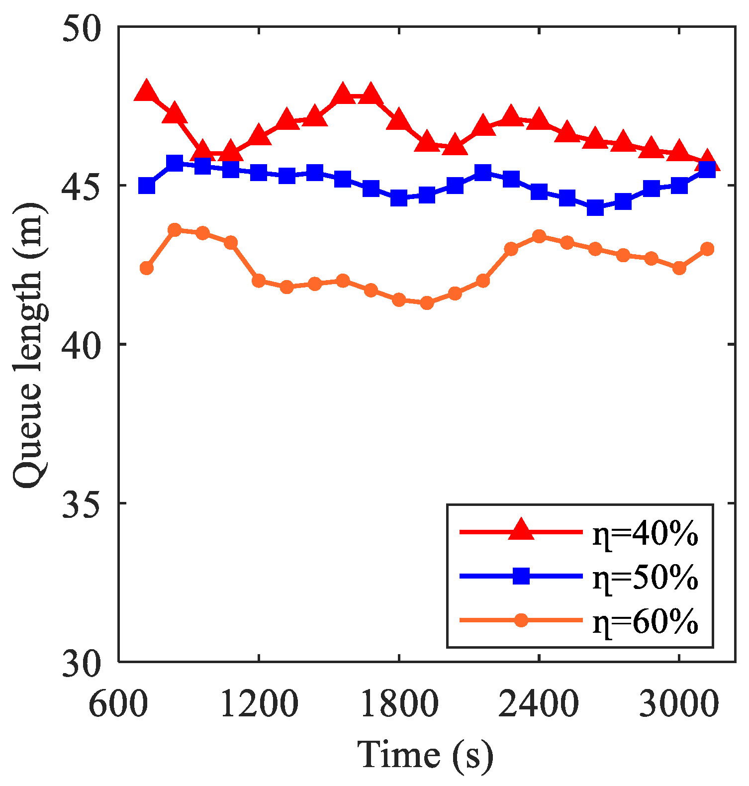
- Queue length
- (3)
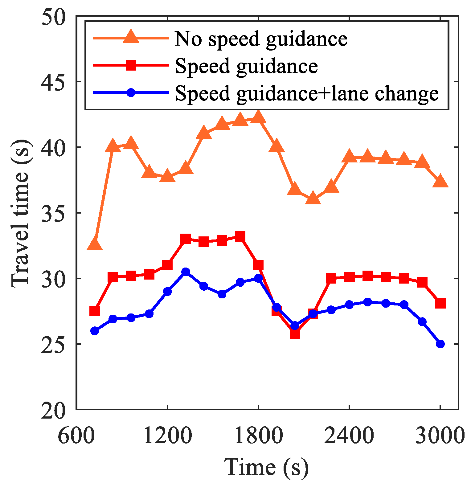
- Vehicle travel time t
5. Conclusions
Author Contributions
Funding
Institutional Review Board Statement
Informed Consent Statement
Data Availability Statement
Conflicts of Interest
References
- Yang, S.; Wang, W.; Lu, C.; Gong, J.; Xi, J. A Time-Efficient Approach for Decision-Making Style Recognition in Lane-Changing Behavior. IEEE Trans. Hum.-Mach. Syst. 2019, 49, 579–588. [Google Scholar] [CrossRef]
- Li, L.; Gan, J.; Zhou, K.; Qu, X.; Ran, B. A novel lane-changing model of connected and automated vehicles: Using the safety potential field theory. Phys. A Stat. Mech. Its Appl. 2020, 559, 125039. [Google Scholar] [CrossRef]
- Wang, Z.; Zhao, X.; Chen, Z.; Li, X. A dynamic cooperative lane-changing model for connected and autonomous vehicles with possible accelerations of a preceding vehicle. Expert Syst. Appl. 2021, 173, 114675. [Google Scholar] [CrossRef]
- Sueyoshi, F.; Utsumi, S.; Tanimoto, J. Underlying social dilemmas in mixed traffic flow with lane changes. Chaos Solitons Fractals 2022, 155, 111790. [Google Scholar] [CrossRef]
- Wang, Y.; Lyu, N.; Wen, J. Game theory-based mandatory lane change model in intelligent connected vehicles environment. Appl. Math. Model. 2024, 132, 146–165. [Google Scholar] [CrossRef]
- Geng, G.; Cheng, G.; Duan, C.; Jiao, X. Optimal lane-changing and collision avoidance strategy for intelligent vehicles in high-speed driving environments. Veh. Syst. Dyn. 2024, 62, 2632–2660. [Google Scholar] [CrossRef]
- An, G.; Talebpour, A. Vehicle Platooning for Merge Coordination in a Connected Driving Environment: A Hybrid ACC-DMPC Approach. IEEE Trans. Intell. Transp. Syst. 2023, 24, 5239–5248. [Google Scholar] [CrossRef]
- Liu, C.; Liu, Z.; Xu, Z.; Li, X. A multistep cooperative lane change strategy for connected and autonomous vehicle platoons departing from dedicated lanes. Transp. Res. Part C Emerg. Technol. 2024, 165, 104720. [Google Scholar] [CrossRef]
- Ali, Y.; Zheng, Z.; Bliemer, M.C.J. Calibrating lane-changing models: Two data-related issues and a general method to extract appropriate data. Transp. Res. Part C Emerg. Technol. 2023, 152, 104182. [Google Scholar] [CrossRef]
- Liu, Q.; Lin, X.; Li, M.; Li, L.; He, F. Coordinated lane-changing scheduling of multilane CAV platoons in heterogeneous scenarios. Transp. Res. Part C Emerg. Technol. 2023, 147, 103992. [Google Scholar] [CrossRef]
- Zhang, H.; Du, L.; Shen, J. Hybrid MPC System for Platoon based Cooperative Lane change Control Using Machine Learning Aided Distributed Optimization. Transp. Res. Part B Methodol. 2022, 159, 104–142. [Google Scholar] [CrossRef]
- He, X.; Yang, H.; Hu, Z.; Lv, C. Robust Lane Change Decision Making for Autonomous Vehicles: An Observation Adversarial Reinforcement Learning Approach. IEEE Trans. Intell. Veh. 2023, 8, 184–193. [Google Scholar] [CrossRef]
- Du, L.; Chen, W.; Ji, J.; Pei, Z.; Tong, B.; Zheng, H. A Novel Intelligent Approach to Lane-Change Behavior Prediction for Intelligent and Connected Vehicles. Comput. Intell. Neurosci. 2022, 2022, 9516218. [Google Scholar] [CrossRef] [PubMed]
- Liu, S.; Wang, X.; Liu, Y.; Chen, L.; Li, H.; Wang, G.; Li, Q. Lane Selection Model Based on Phase-Field Coupling and Set Pair Logic. J. Transp. Eng. Part A Syst. 2022, 148, 04022097. [Google Scholar] [CrossRef]
- Zheng, Y.; Ran, B.; Qu, X.; Zhang, J.; Lin, Y. Cooperative Lane Changing Strategies to Improve Traffic Operation and Safety Nearby Freeway Off-Ramps in a Connected and Automated Vehicles Environment. IEEE Trans. Intell. Transp. Syst. 2020, 21, 4605–4614. [Google Scholar] [CrossRef]
- Wang, Y.; Lyu, N.; Wen, J. Modeling risk potential fields for mandatory lane changes in intelligent connected vehicle environment. Expert Syst. Appl. 2024, 255, 124814. [Google Scholar] [CrossRef]
- Peng, J.; Wei, S.; Chai, L. Strategy of lane-changing coupling process for connected and automated vehicles in mixed traffic environment. Transp. B Transp. Dyn. 2023, 11, 979–995. [Google Scholar] [CrossRef]
- Zhai, C.; Wu, W.T.; Xiao, Y.P. The jamming transition of multi-lane lattice hydrodynamic model with passing effect. Chaos Solitons Fractals 2023, 171, 113515. [Google Scholar] [CrossRef]
- Zhai, C.; Wu, W.T.; Xiao, Y.P. Cooperative car-following control with electronic throttle and perceived headway errors on gyroidal roads. Appl. Math. Model. 2022, 108, 770–786. [Google Scholar] [CrossRef]
- Zhai, C.; Li, K.N.; Zhang, R.H.; Peng, T.; Zong, C.F. Phase diagram in multi-phase heterogeneous traffic flow model integrating the perceptual range difference under human-driven and connected vehicles environment. Chaos Solitons Fractals 2024, 182, 114791. [Google Scholar] [CrossRef]
- Tumminello, M.L.; Macioszek, E.; Granà, A.; Giuffrè, T. Evaluating Traffic-Calming-Based Urban Road Design Solutions Featuring Cooperative Driving Technologies in Energy Efficiency Transition for Smart Cities. Energies 2023, 16, 7325. [Google Scholar] [CrossRef]
- Choi, S.; Lee, D.; Kim, S.; Tak, S. Framework for connected and automated bus rapid transit with sectionalized speed guidance based on deep reinforcement learning: Field test in Sejong city. Transp. Res. Part C Emerg. Technol. 2023, 148, 104049. [Google Scholar] [CrossRef]
- Khayyat, M.; Gabriele, A.; Mancini, F.; Arrigoni, S.; Braghin, F. Enhanced Traffic Light Guidance for Safe and Energy-Efficient Driving: A Study on Multiple Traffic Light Advisor (MTLA) and 5G Integration. J. Intell. Robot. Syst. 2024, 110, 73. [Google Scholar] [CrossRef]
- Wang, T.; Yuan, Z.; Zhang, Y.; Zhang, J.; Tian, J. A driving guidance strategy with pre-stop line at signalized intersection: Collaborative optimization of capacity and fuel consumption. Phys. A Stat. Mech. Its Appl. 2023, 626, 129068. [Google Scholar] [CrossRef]
- Wu, R.; Jia, H.; Huang, Q.; Tian, J.; Gao, H.; Wang, G. Multi-Lane Unsignalized Intersection Cooperation Strategy Considering Platoons Formation in a Mixed Connected Automated Vehicles and Connected Human-Driven Vehicles Environment. IEEE Trans. Intell. Transp. Syst. 2024, 25, 1569–1585. [Google Scholar] [CrossRef]
- Zhou, A.; Peeta, S.; Wang, J. Cooperative control of a platoon of connected autonomous vehicles and unconnected human-driven vehicles. Comput.-Aided Civ. Infrastruct. Eng. 2023, 38, 2513–2536. [Google Scholar] [CrossRef]
- Fu, Y.; Li, C.; Luan, T.H.; Zhang, Y. IoV and blockchain-enabled driving guidance strategy in complex traffic environment. China Commun. 2023, 20, 230–243. [Google Scholar] [CrossRef]
- Ren, C.; Wang, Z.; Yin, C.; Xu, H.; Wang, L.; Guo, L.; Li, J. Boundary guidance strategy and method for urban traffic congestion region management in internet of vehicles environment. J. Adv. Transp. 2023, 2023, 4866326. [Google Scholar] [CrossRef]
- Chen, J.; Hu, M.; Shi, C. Development of eco-routing guidance for connected electric vehicles in urban traffic systems. Phys. A Stat. Mech. Its Appl. 2023, 618, 128718. [Google Scholar] [CrossRef]
- Wu, H.; Zhou, H.; Zhao, J.; Xu, Y.; Qian, B.; Shen, X. Deep learning enabled fine-grained path planning for connected vehicular networks. IEEE Trans. Veh. Technol. 2022, 71, 10303–10315. [Google Scholar] [CrossRef]
- Yao, Z.; Jin, Y.; Jiang, H.; Hu, L.; Jiang, Y. CTM-based traffic signal optimization of mixed traffic flow with connected automated vehicles and human-driven vehicles. Phys. A Stat. Mech. Its Appl. 2022, 603, 127708. [Google Scholar] [CrossRef]
- Yao, H.; Li, X. Decentralized control of connected automated vehicle trajectories in mixed traffic at an isolated signalized intersection. Transp. Res. Part C Emerg. Technol. 2020, 121, 102846. [Google Scholar] [CrossRef]
- Huang, Y.; Wang, Y.; Yan, X.; Duan, K.; Zhu, J. Behavior model and guidance strategies of the crossing behavior at unsignalized intersections in the connected vehicle environment. Transp. Res. Part F Traffic Psychol. Behav. 2022, 88, 13–24. [Google Scholar] [CrossRef]
- Bifulco, G.N.; Coppola, A.; Petrillo, A.; Santini, S. Decentralized cooperative crossing at unsignalized intersections via vehicle-to-vehicle communication in mixed traffic flows. J. Intell. Transp. Syst. 2022, 28, 211–236. [Google Scholar] [CrossRef]
- Wu, S.; Chen, Z.; Shen, S.; Shen, J.; Guo, F.; Liu, Y.; Zhang, Y. Hierarchical cooperative eco-driving control for connected autonomous vehicle platoon at signalized intersections. IET Intell. Transp. Syst. 2023, 17, 1560–1574. [Google Scholar] [CrossRef]
- Coppola, A.; Di Costanzo, L.; Pariota, L.; Santini, S.; Bifulco, G.N. An Integrated Simulation Environment to test the effectiveness of GLOSA services under different working conditions. Transp. Res. Part C Emerg. Technol. 2022, 134, 103455. [Google Scholar] [CrossRef]
- Liu, M.; Zhao, J.; Hoogendoorn, S.; Wang, M. A single-layer approach for joint optimization of traffic signals and cooperative vehicle trajectories at isolated intersections. Transp. Res. Part C Emerg. Technol. 2022, 134, 103459. [Google Scholar] [CrossRef]
- Zhao, J.; Knoop, V.L.; Wang, M. Microscopic traffic modeling inside intersections: Interactions between drivers. Transp. Sci. 2023, 57, 135–155. [Google Scholar] [CrossRef]
- Zhao, J.; Knoop, V.L.; Sun, J.; Ma, Z.; Wang, M. Unprotected Left-Turn Behavior Model Capturing Path Variations at Intersections. IEEE Trans. Intell. Transp. Syst. 2023, 24, 9016–9030. [Google Scholar] [CrossRef]
- Leutzbach, W.; Wiedemann, R. Development and applications of traffic simulation models at the karlsruhe institut fuer verkehrswesen. Traffic Eng. Control 1986, 27, 270–278. [Google Scholar]
- Kometani, E.; Sasaki, T. On the Stability of Traffic Flow. J. Opns. Res. Jpn. 1958, 2, 11–26. [Google Scholar]
- Bando, M.; Hasebe, K.; Nakayama, A.; Shibata, A.; Sugiyama, Y. Dynamical model of traffic congestion and numerical simulation. Phys. Rev. E 1995, 51, 1035–1042. [Google Scholar] [CrossRef] [PubMed]
- Helbing, D.; Tilch, B. Generalized force model of traffic dynamics. Phys. Rev. E 1998, 58, 133–138. [Google Scholar] [CrossRef]
- Duan, X.; Sun, C.; Tian, D.; Zhou, J.; Cao, D. Cooperative Lane-Change Motion Planning for Connected and Automated Vehicle Platoons in Multi-Lane Scenarios. IEEE Trans. Intell. Transp. Syst. 2023, 24, 7073–7091. [Google Scholar] [CrossRef]
- Monteiro, F.V.; Ioannou, P. Safe autonomous lane changes and impact on traffic flow in a connected vehicle environment. Transp. Res. Part C Emerg. Technol. 2023, 151, 104138. [Google Scholar] [CrossRef]


| Description | Symbol | Unit |
|---|---|---|
| The speed at which a vehicle enters the speed zone | v0 | m/s |
| The time at which a vehicle enters the speed zone | t0 | s |
| The reaction time taken to execute the command | ∆t | s |
| The maximum (low) speed limit of the lane | vmax/vmin | m/s |
| The comfortable acceleration (or deceleration) of the vehicle | a | m/s2 |
| The color of the light when entering the speed guidance zone | Light | G/R |
| The remaining time at the end of the green light | tg/tr | s |
| The guidance speed | vsug | m/s |
| The length of the speed guidance zone | L | m |
| The length of the queue at an intersection | l | m |
| The vehicle safety spacing | ds | m |
| The speed of smooth traffic | vf | m/s |
| The speed at which a queue dissipates | vp | m/s |
| North | East | South | West | ||||
|---|---|---|---|---|---|---|---|
| Inlet Road | Exit Road | Inlet Road | Exit Road | Inlet Road | Exit Road | Inlet Road | Exit Road |
| 2 lanes | 1 straight left | 2 lanes | 1 left | 2 lanes | 1 left | 3 lanes | 1 left |
| 1 straight right | 1 straight | 1 straight | 1 straight | ||||
| 1 straight right | 1 right | 1 straight right | |||||
| Plan | Cycle | Phase 1 | Phase 2 | Phase 3 | Phase 4 | ||||
|---|---|---|---|---|---|---|---|---|---|
| 1 | 140 | East–west straight ahead at the same time | 28 | East–west left turn at the same time | 26 | North–south straight ahead at the same time | 32 | North left turn and south right turn release | 30 |
| 2 | 80 | The eastern and western phases are released simultaneously | 38 | The northern and southern phases are released simultaneously | 30 | ||||
| 3 | 60 | The eastern and western phases are released simultaneously | 26 | The northern and southern phases are released simultaneously | 22 | ||||
| Description | Value |
|---|---|
| Length of metacells (i)/m | 7.5 |
| Number of metacells (N)/grid-lane−1 | 1000 |
| Social vehicle speed (Vs)/grid-step | 0~3 |
| Emergency vehicle speed (Ve)/grid-step | 0~5 |
| Traffic density (ρ) | 0~1 |
| Time step | 10,000 |
| The weight coefficient | 0.5 |
| The weight coefficient | 0.5 |
| Name | Definition |
|---|---|
| Algorithm 2 | As mentioned in [11] |
| Algorithm 3 | As mentioned in [12] |
| Algorithm 2 | Algorithm 3 | The Proposed Method | |
|---|---|---|---|
| Optimal solution | 80.13% | 88.48% | 95.65% |
| Computational performance (s) | 12.20 | 5.74 | 1.29 |
Disclaimer/Publisher’s Note: The statements, opinions and data contained in all publications are solely those of the individual author(s) and contributor(s) and not of MDPI and/or the editor(s). MDPI and/or the editor(s) disclaim responsibility for any injury to people or property resulting from any ideas, methods, instructions or products referred to in the content. |
© 2025 by the authors. Licensee MDPI, Basel, Switzerland. This article is an open access article distributed under the terms and conditions of the Creative Commons Attribution (CC BY) license (https://creativecommons.org/licenses/by/4.0/).
Share and Cite
Dong, L.; Xie, X.; Zhang, L.; Cheng, X.; Qiu, B. Satisfaction-Based Optimal Lane Change Modelling of Mixed Traffic Flow and Intersection Vehicle Guidance Control Method in an Intelligent and Connected Environment. Sustainability 2025, 17, 1077. https://doi.org/10.3390/su17031077
Dong L, Xie X, Zhang L, Cheng X, Qiu B. Satisfaction-Based Optimal Lane Change Modelling of Mixed Traffic Flow and Intersection Vehicle Guidance Control Method in an Intelligent and Connected Environment. Sustainability. 2025; 17(3):1077. https://doi.org/10.3390/su17031077
Chicago/Turabian StyleDong, Luxi, Xiaolan Xie, Lieping Zhang, Xiaohui Cheng, and Bin Qiu. 2025. "Satisfaction-Based Optimal Lane Change Modelling of Mixed Traffic Flow and Intersection Vehicle Guidance Control Method in an Intelligent and Connected Environment" Sustainability 17, no. 3: 1077. https://doi.org/10.3390/su17031077
APA StyleDong, L., Xie, X., Zhang, L., Cheng, X., & Qiu, B. (2025). Satisfaction-Based Optimal Lane Change Modelling of Mixed Traffic Flow and Intersection Vehicle Guidance Control Method in an Intelligent and Connected Environment. Sustainability, 17(3), 1077. https://doi.org/10.3390/su17031077