Article

Tidal Current Modeling Using Shallow Water Equations Based on the Finite Element Method: Case Studies in the Qiongzhou Strait and Around Naozhou Island

by
Dawei Peng
1,
Jia Mao
1,
Jianhua Li
2 and
Lanhao Zhao
1,*
1
College of Water Conservancy and Hydropower Engineering, Hohai University, Nanjing 210024, China
2
China Energy Engineering Group Guangdong Electric Power Design Institute Co., Ltd., Guangzhou 510663, China
*
Author to whom correspondence should be addressed.
Sustainability 2025, 17(3), 1256; https://doi.org/10.3390/su17031256
Submission received: 5 January 2025 / Revised: 23 January 2025 / Accepted: 26 January 2025 / Published: 4 February 2025

Abstract

:
Tidal currents are a crucial oceanic process with significant implications for marine engineering and the sustainable use of coastal and marine resources. This paper presents the development of a finite element numerical model to simulate tidal currents. The model was mathematically formulated using the shallow water equations, which are applicable to fluid dynamics where the horizontal scale is significantly larger than the vertical scale. The finite element method was employed to discretize and solve the equations, with the bottom slope source term incorporated into the pressure equation to ensure numerical consistency. Furthermore, characteristic line theory was applied to derive the relationship between boundary tidal levels and current velocities to satisfy boundary compatibility conditions. The model was initially applied to the Qiongzhou Strait, and the results demonstrated good agreement with observed data. Subsequently, the model was implemented at Naozhou Island and its adjacent waters. The results revealed that the tidal currents around Naozhou Island exhibit oscillatory flow patterns, with the flow direction near Donghai Island oriented northeast–southwest (NE-SW) and the flow direction near Leizhou Bay oriented northwest–southeast (NW-SE). This study provides a hydrodynamic basis for marine engineering projects and the sustainable utilization of marine resources in the Naozhou Island area.

1. Introduction

Tidal currents are one of the most critical dynamic forces in the marine environment and have a significant influence on ocean circulation, mixing processes, and the design, construction, and operation of marine engineering projects [1]. In the South China Sea, particularly in coastal regions, the tidal currents would directly impact local engineering projects, fisheries management, and economic activities. Therefore, a thorough understanding of tidal movements and their underlying mechanisms is essential. While coastal estuarine tidal currents exhibit three-dimensional characteristics, their horizontal scales substantially exceed their vertical scales. Consequently, to simplify the computational complexity, the three-dimensional Navier–Stokes equations, which govern fluid motion, can be vertically integrated. As a result, tidal flows can then be effectively approximated using two-dimensional shallow water equations (SWEs).
Numerical simulations of tidal currents utilizing SWEs have been explored through various methodologies, which include the Finite Difference Method (FDM) [2,3], Finite Volume Method (FVM) [4,5], Discontinuous Galerkin Method (DGM) [6,7], and Finite Element Method (FEM) [8,9,10,11]. It is worth noting that the FEM was first applied by Grotkop [12] in 1973 for solving the two-dimensional SWEs. Thereafter, the FEM has been effectively applied in numerous tidal current studies due to its rigorous mathematical foundation and its ability to accurately handle complex geometries and boundary conditions.
Numerical simulations using SWEs present two significant challenges: numerical stability with constantly changing ground elevations and the accurate treatment of wet–dry interface conditions [13]. The former is also known as the ‘C-property’ or ‘well-balanced property’, which was initially introduced by Bermudez [14]. An improper splitting of the surface gradient into flux gradient and bed slope terms can introduce numerical imbalance, which may compromise the well-balanced nature of the scheme [15]. The latter challenge is the transition between dry and wet regions. Failure to adequately handle the drying–wetting front can result in numerical instabilities or inaccurate computations near these interfaces when using standard numerical methods, which may generate unacceptably negative water heights [16]. Several well-balanced schemes for SWEs, such as flux modification, Riemann solvers, and exact Riemann solvers, have been proposed in the literature [2,3,4]. Methods for handling drying and wetting have also been developed [6,17,18,19]. These advancements provide a theoretical foundation for numerical simulation of tidal currents.
So far, the SWEs have been widely applied in numerical simulations of tides in marine and estuarine areas. Rompas [20] used a semi-implicit finite difference method to solve the SWEs, and simulated the ocean currents in the Bunaken Strait in North Sulawesi Province, Indonesia. Barth [21] presented a method for generating an ensemble of perturbations that satisfy prescribed linear dynamical constraints, which was applied to the West Florida Shelf. Walters [22] employed an unstructured-grid numerical model to simulate tides and currents in Cook Strait, New Zealand. Le [23] introduced an implicit wetting–drying algorithm implemented in the SLIM model, which was applied to the Tonle Sap Lake in the Mekong River Basin. Zhang [24] investigated tide–surge interactions induced by Typhoon Mangkhut (2018) in the Pearl River Estuary during typhoon seasons, and the investigation was based on finite volume SWEs, aiming to provide extreme sea level estimates for coastal engineering. Peng [25] employed a GPU-accelerated and Local Time Step-based FVM, which was applied in three scenarios: an idealized dam-break flow, an experimental dam-break flow, and tidal flows in the Yangtze estuary. Chen [26] introduced a wetting and drying method for a three-dimensional discontinuous Galerkin hydrodynamic model, which was applied to simulate tidal currents in Laizhou Bay. Su [27] developed a new numerical model based on non-linear SWEs to simulate and predict tidal bores in the Hangzhou Gulf and Qiantang River, and the model was validated against analytical solutions and experimental data. He [28] employed geostationary satellite ocean color data in conjunction with SWEs to simulate sediment transport and sedimentation processes in Lake Taihu.
In previous studies on tidal current simulation, FDM, FVM, and DGM have been widely used. However, for hydrodynamic simulations with complex geometric boundaries, the FEM has distinct advantages. FEM employs unstructured grids (such as triangular or quadrilateral grids), which can flexibly adapt to complex coastlines and terrain changes. And the problems like grid distortion and accuracy loss can be avoided. Furthermore, FEM also has advantages in handling high-order accuracy problems and complex boundary conditions. Therefore, FEM was adopted in this study to solve the SWEs.
Within the finite element framework, the governing equations were discretized using a characteristic Galerkin procedure. Furthermore, a tidal open boundary condition based on characteristic line theory was implemented for tidal current calculations. To validate the accuracy of the proposed method, tidal currents in the Qiongzhou Strait were firstly simulated, which confirmed the reliability of the present method for marine tidal modeling. Subsequently, the method was extended to the area surrounding Naozhou Island in the South China Sea, where tidal currents were computed, and a detailed analysis of their characteristics was performed. Accurate tidal simulations are crucial for the sustainable use of marine resources, such as tidal energy development and port construction. The model proposed in this study improves the accuracy and efficiency of tidal simulations, providing a more reliable basis for the planning and decision-making of related projects.

2. Numerical Method

2.1. Governing Equations

In a two-dimensional plane model, the water flow is considered as an incompressible Newtonian fluid. The SWEs, derived by vertically integrating the Navier–Stokes equations over the water depth, are employed as the governing equations. This model accounts for surface wind shear stress and the Coriolis force, including the continuity equation and the momentum equation in Cartesian coordinates.
h t + · U = 0
U t + · ( u U ) = · τ p + S b + S
where h is the total water depth, t is the time, and is the horizontal gradient operator. U = u h is the conserved variable, the components in x and y directions are U x and U b , and u is the depth-averaged horizontal velocity. τ = h ν ( u + T u ) is the viscous term, and ν is the kinematic viscosity coefficient. p = g h 2 / 2 is the pressure term, and g is the gravity acceleration. S b = g h z is the bed slope term and S = τ c + 1 ρ τ s 1 ρ τ b is the remaining terms, where z is the elevation of bottom. τ c = f c U is the Coriolis force, where f c = 2 ω sin φ is the Coriolis coefficient, ω is the earth rotation frequency, and φ is local latitude. τ s = ρ a C w | w | w is the surface wind stress, where ρ a is the density of air, C w is the empirical drag coefficient of air, and w is wind speed at 10 m above water surface. τ b = g n 2 | u | u h 1 3 is the bottom friction.

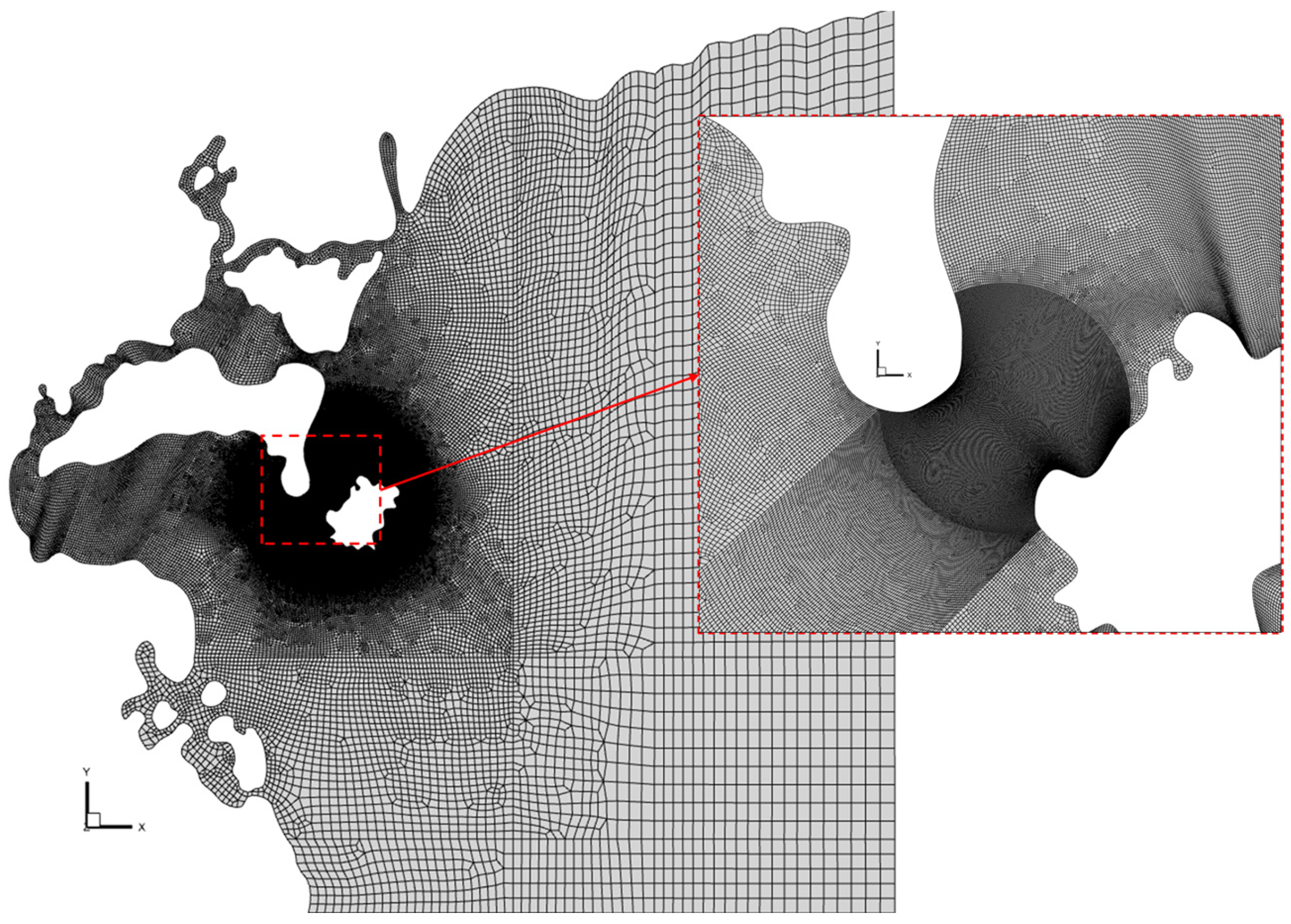
2.2. Numerical Discretization

This study employs a splitting method based on the characteristic-based split scheme [29], combined with an explicit time-stepping scheme, to decompose Equations (1) and (2) into a series of easier-to-solve sub-steps, thereby avoiding the direct solution of the nonlinear equations. Defining the wave speed c = g h , and introducing two parameters θ 1 , θ 2 , the governing equations are rewritten in the following time-discretized form:
1 c 2 Δ p Δ t + · U n + θ 1 = 0
Δ U Δ t + · ( u U ) = · τ p n + θ 2 + S b + S
Here, the parameter θ 1 and θ 2 can be chosen in the range [0,1]. 1 / 2 θ 1 1 , 1 / 2 θ 2 1 for the semi-implicit form, and 1 / 2 θ 1 1 , θ 2 = 0 for an explicit form.
Defining F = u U , G = τ , Q = S , Equation (4) is rewritten in a general conservative equation form:
U t + · F + · G + Q = 0
According to the characteristic-based split scheme [29], the time discretization of Equation (5) along the characteristic line gives
Δ U = Δ t 2 2 u · ( · F + Q ) n Δ t ( · F + · G + Q ) n + Δ t 2 2 u · ( p n + θ 2 S b ) Δ t ( p n + θ 2 S b )
Following the fractional step procedure proposed by Chorin [30], the increment Δ U can be decomposed into two parts:
Δ U = Δ U + Δ U #
Δ U = Δ t 2 2 u · ( · F + Q ) n Δ t ( · F + · G + Q ) n
Δ U # = Δ t 2 2 u · ( p n + θ 2 S b ) Δ t ( p n + θ 2 S b )
Initially, the increment of intermediate variable Δ U is explicitly determined by excluding the pressure gradient and bed slope terms. Subsequently, U is adjusted to account for pressure effects once the pressure increment Δ p n is derived from the Poisson equation either implicitly or explicitly. This process yields the increment variable Δ U # , ultimately leading to the final value of Δ U .
Step 1: Intermediate variable.
The increment of intermediate variable Δ U is obtained from Equation (8). According to the standard Galerkin approximation, Equation (8) is discretized in space as:
N T N d Ω Δ U ¯ = Δ t N T G · n d Γ Δ t [ N T ( · F + Q ) d Ω N T · G d Ω ] Δ t 2 2 · ( N T u ) ( · F + Q ) d Ω
where U ¯ and N represent the nodal values and shape function of the velocity field, respectively.
Step 2: Pressure equation.
It is worth noting that, to ensure the numerical solution’s consistency, the calculation of the increment of the intermediate conservative variable excludes the influences of the pressure term and bed slope term. These effects are incorporated into the resolution of the pressure equation by merging the pressure gradient term and bed slope term:
Δ U # = Δ t ( p n + θ 2 S b )
Substituting U n + θ 1 = U n + θ 1 Δ U + θ 1 Δ U # to the continuity Equation (3) at time t n + θ 1 gives
1 c 2 Δ p Δ t + · [ U n + θ 1 Δ U θ 1 Δ t ( p n + θ 2 S b ) ] = 0
By employing standard finite element shape functions for spatial approximation and applying integration by parts according to the Green’s theorem, the discretized pressure equation can be obtained.
Δ p ¯ n N p T 1 c 2 N p d Ω + Δ p ¯ n θ 1 θ 2 Δ t 2 N T · N d Ω = Δ t N p T · ( U n + θ 1 Δ U ) d Ω θ 1 Δ t 2 N p T · ( p n S b ) d Ω + θ 1 Δ t 2 N p T ( p n + θ 2 S b ) · n d Γ
where N p is the shape function scalar for the pressure field. Δ p ¯ n is the nodal pressure increment.
Step 3: Increment correction.
Modify U by Equation (9) with the pressure obtained from the previous step:
N T N d Ω Δ U ¯ # = Δ t N T [ ( p n + θ 2 Δ p n ) S b ] d Ω
The governing equations have now been transferred to the discretization form with the finite element method in Equations (10), (13), and (14).

2.3. Tidal Open Boundary Conditions

Due to the practical limitations of tidal flow observations, precise tide level information is typically available, while accurately determining flow velocities remains challenging. As a result, flow velocity data are often insufficient, even when boundary conditions are provided. In scenarios where the Froude number is less than 1, indicating a tranquil flow state, the tide level information at the boundaries must adhere to compatibility conditions to avoid disrupting the upstream flow regime. This section derives boundary flow velocity values that meet compatibility conditions based on the characteristics of the flow theory.
For a two-dimensional boundary, a common approach is to treat it as a one-dimensional boundary by locally approximating along the normal direction to the boundary. The boundary flow velocity can be directly calculated by the boundary water level. Therefore, there is no need for iterative solving. According to one-dimensional characteristic line theory, there exist left and right characteristic invariants, denoted as R + and R , respectively.
R + = u 2 c ,   R = u + 2 c
{ d d t ( u 2 c ) = 0 ,   d x d t = u c d d t ( u + 2 c ) = 0 ,   d x d t = u + c
For the boundary, if the left side lies within the computational domain, then the right characteristic invariant remains constant along the characteristic line and the normal flow velocity u L and wave speed c L at the interior points on the left side of the boundary satisfy the following relationship with the normal flow velocity u and wave speed c on the boundary:
u L + 2 c L = u + 2 c
Similarly, if the right side of the boundary lies within the computational domain, then the left characteristic invariant along the characteristic line could be written as:
u R 2 c R = u 2 c
Here, u R and c R represent the normal flow velocity and wave speed at the interior points on the right side of the boundary, respectively. Based on Equations (17) and (18), open boundaries can be effectively handled to ensure the compatibility of boundary variables. Taking the scenario where the right side of the boundary lies within the computational domain as an example to illustrate determining the boundary flow velocity given the known boundary water level, when the water level on the boundary is given as h ( t ) = h , the wave speed can be obtained as c = g h . According to Equation (18), the normal flow velocity on the boundary is then calculated as
u = R + + 2 c

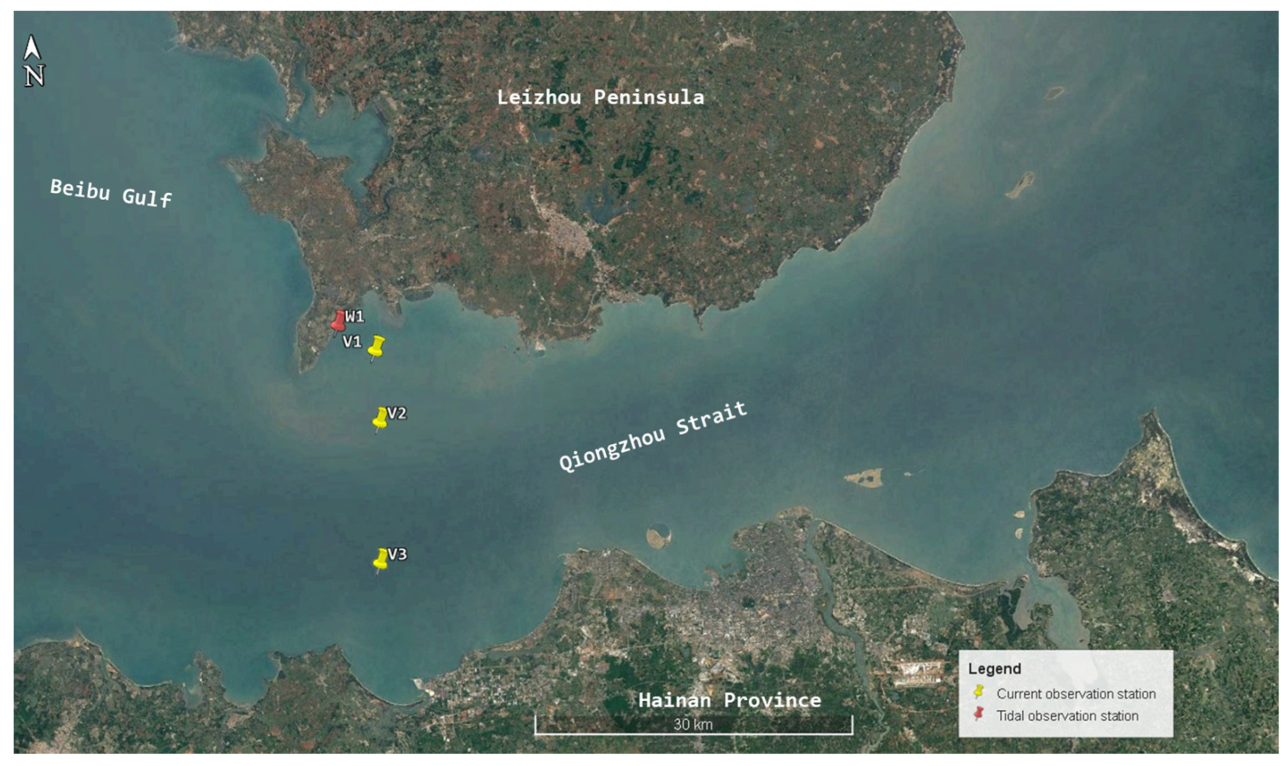
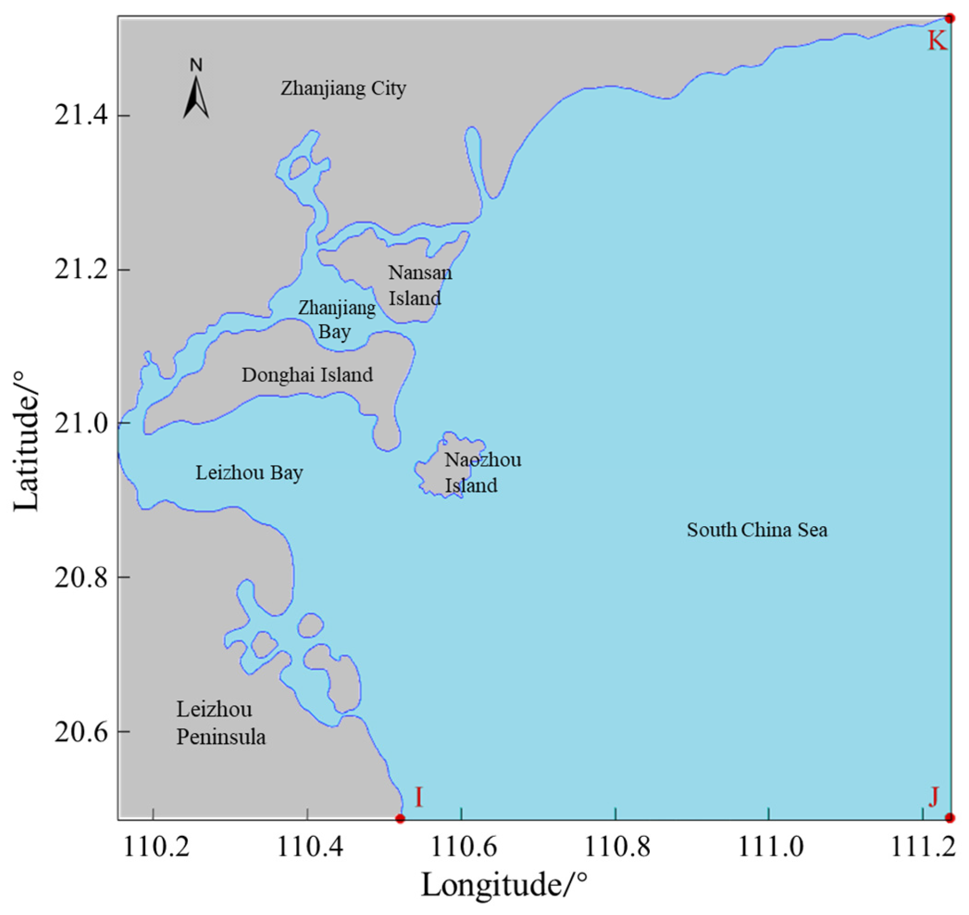
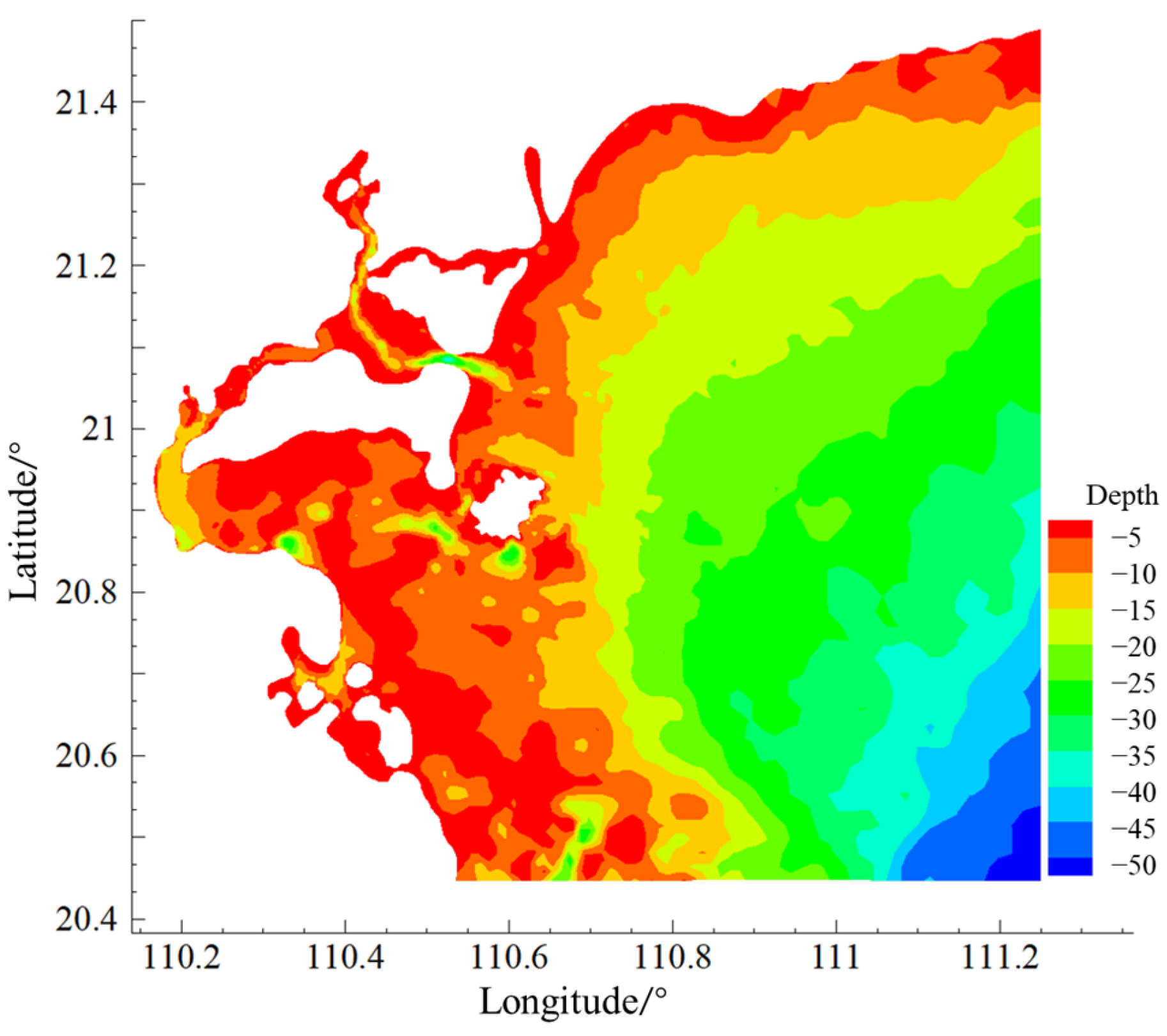
3. Research Area and Data Sources

The main computational domain for this calculation included Naozhou Island and the Qiongzhou Strait region. Coastline and topographic information are direct factors influencing the accuracy of tidal predictions. Therefore, high-resolution coastline and bathymetric data are essential for tidal simulations. In this study, coastline data with a resolution of 10 m were obtained from the Global Self-consistent, Hierarchical, High-resolution Geography Database (GSHHG) (http://www.soest.hawaii.edu/pwessel/gshhg/, accessed on 10 October 2020), and bathymetric data with a resolution of 15 arc-seconds were obtained from the General Bathymetric Chart of the Oceans (GEBCO) (https://www.gebco.net/data_and_products/gridded_bathymetry_data/, accessed on 5 February 2021) 2021 dataset, a globally recognized bathymetric data initiative ensuring long-term sustainability for marine science.
It is important to note that the model calculation maps used below do not fully represent the actual coastline of the South China Sea. For computational convenience, the coastline data obtained from the GSHHG were smoothed. Additionally, some small islands near the boundary, which could potentially impact the calculations, were excluded from the model.
Field measurement data used in this study were obtained from a project conducted by the China Energy Engineering Group Guangdong Electric Power Design Institute Co., Ltd. (Guangzhou, China). These measurements included a comprehensive dataset covering tidal levels, flow speed, flow directions, as well as other parameters such as water temperature, salinity, and energy spectra. The tide gauge instrument used was the RBRsolo3 D (RBR Ltd., Ottawa, Canada), while the ocean current monitoring instrument was the Seaguard® RCM (Aanderaa, Bergen, Norway). In numerical simulations, the water level information at the open boundary was calculated by DHI MIKE 2020 software or the FES2014 global tidal model [31] so that the water level time series at the open boundary could be obtained, which can be used as the water level boundary conditions. Both the observation stations and information at the open boundary in the model were using the WGS84 coordinate system, and the time was based on Beijing Time (GMT+8).

4. Numerical Experiments

The Qiongzhou Strait and Naozhou Island are important marine ecosystems and economic zones whose sustainable development relies on accurate tidal current information. In this section, the accuracy of the proposed method is validated by comparing the simulation results with observed data.

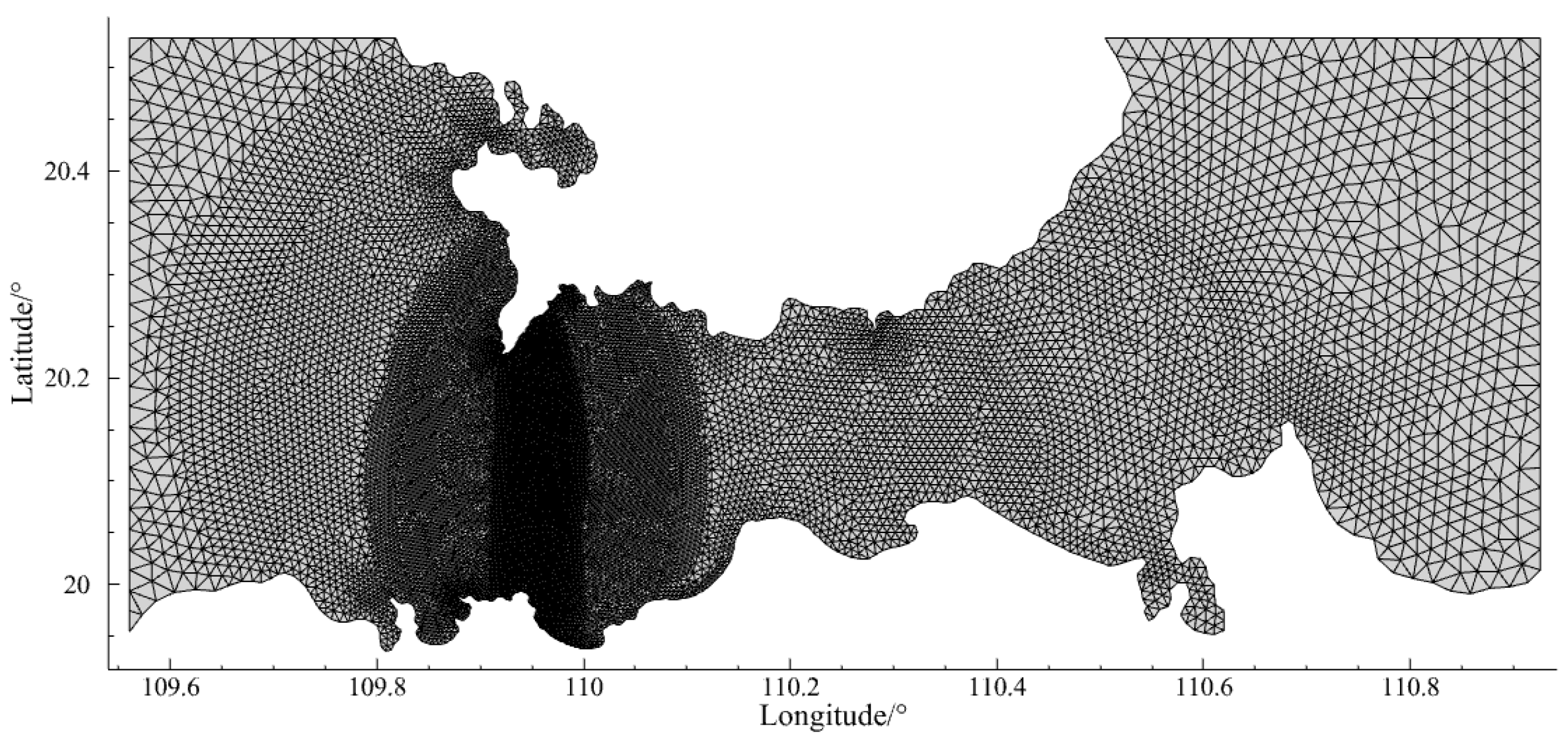
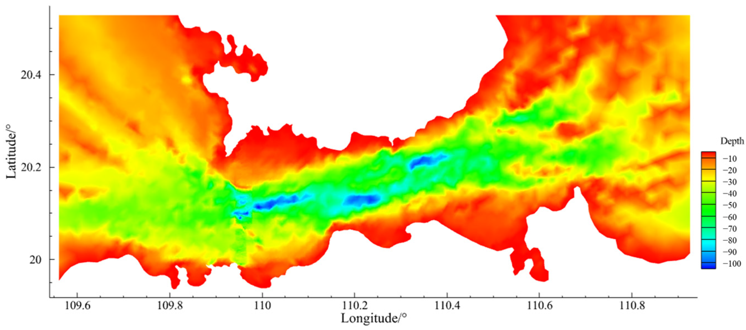
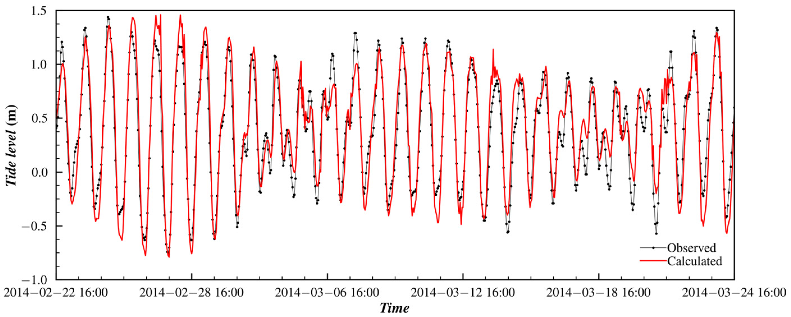
4.1. Qiongzhou Strait
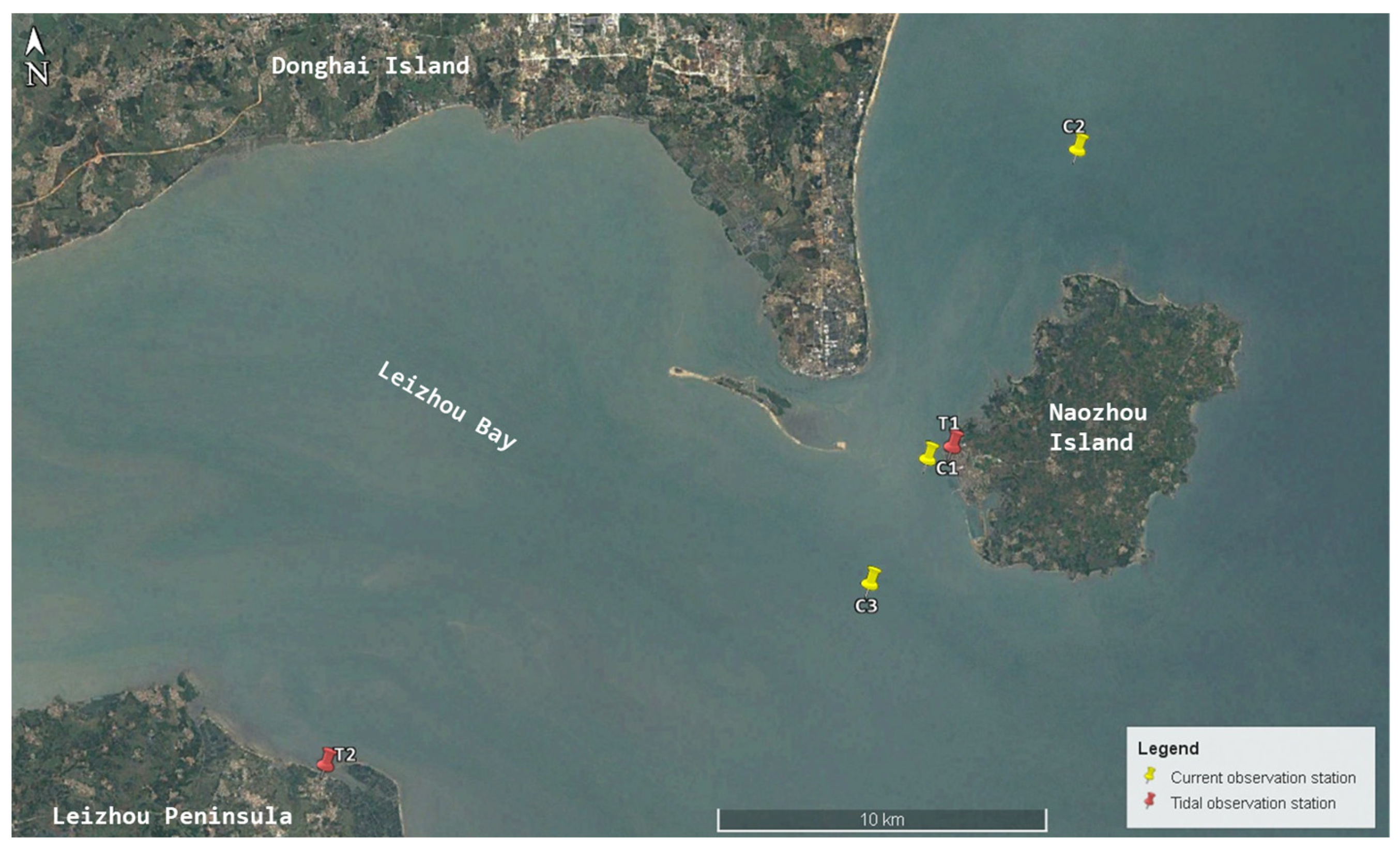
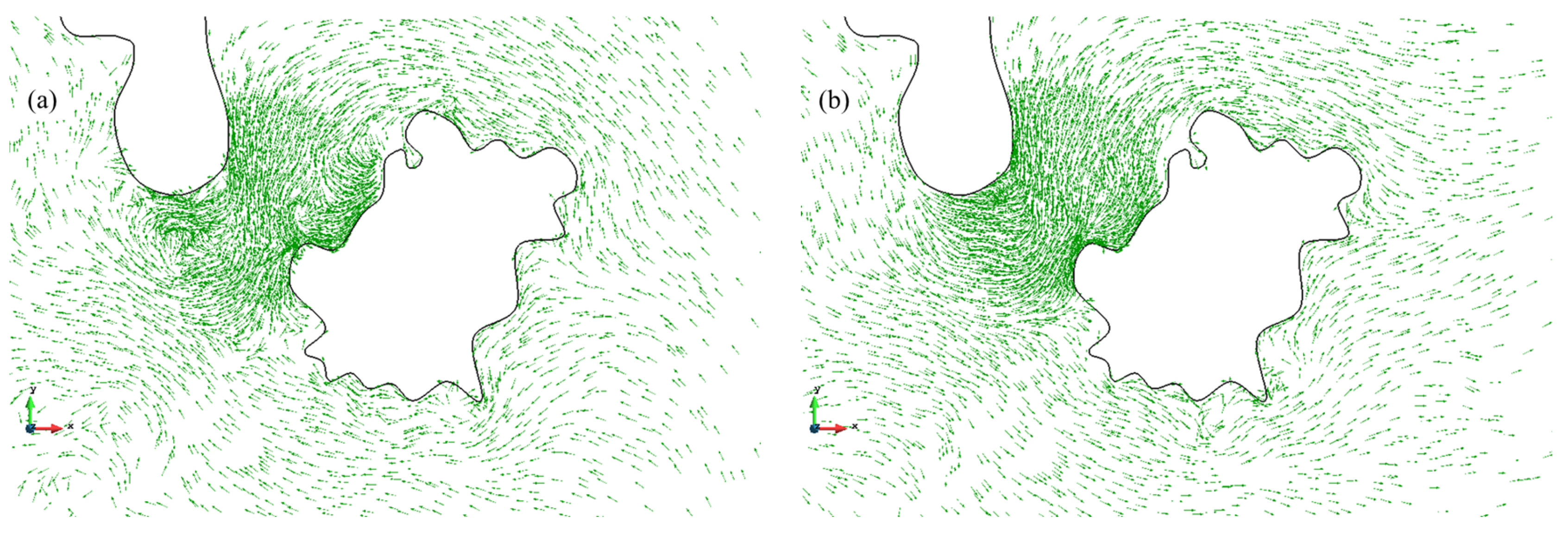
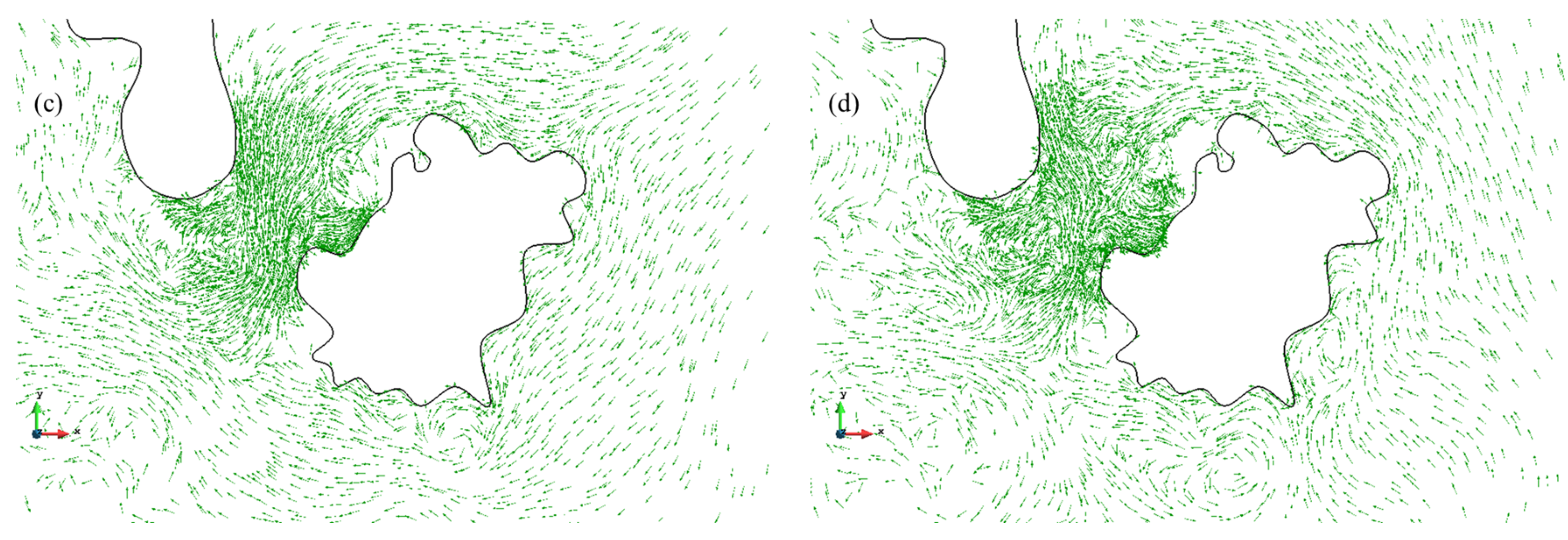
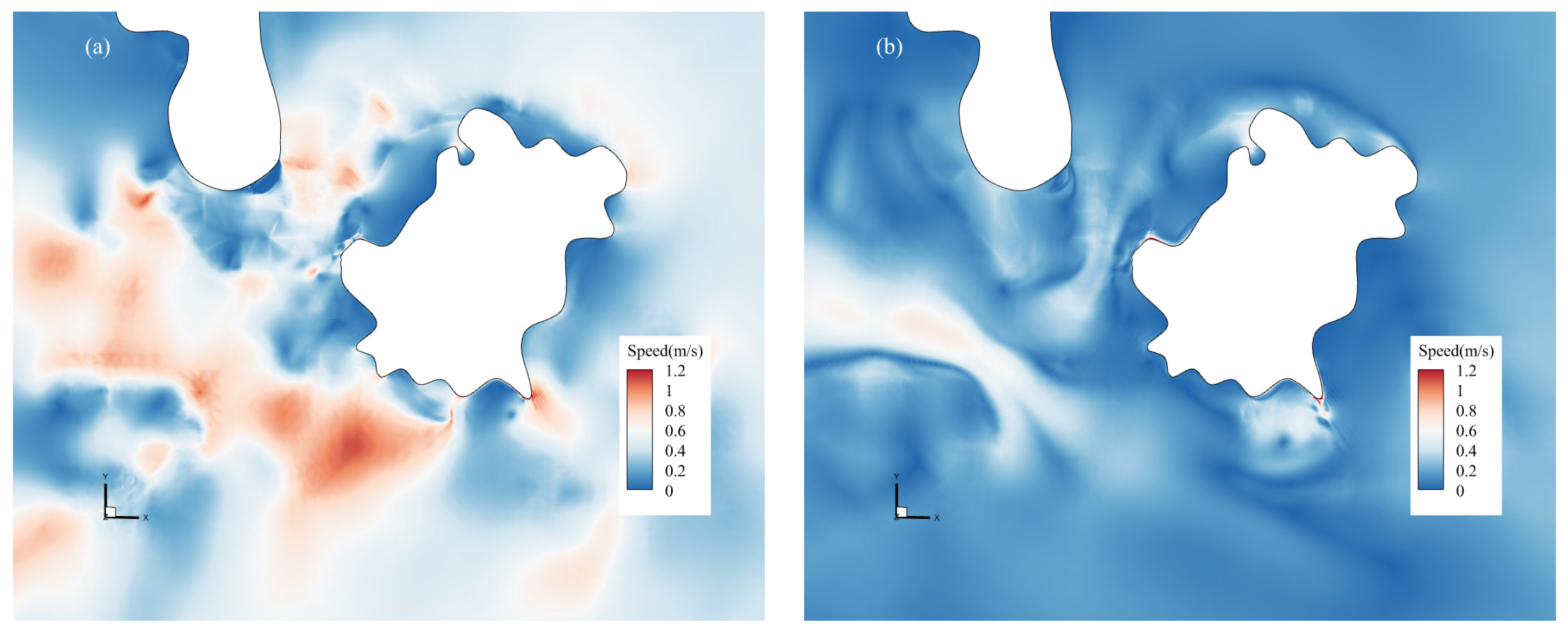
The Qiongzhou Strait is in the inland waters of China, serving as the water passage between Hainan Island and the Leizhou Peninsula in Guangdong Province, as shown in Figure 1. To the east of the Qiongzhou Strait lies the Guangdong Sea area of the South China Sea, while to the west lies the Beibu Gulf. It is a key route for water exchange between the South China Sea and the Beibu Gulf [32]. It spans approximately 80 km from east to west and has an average width of 29.5 km from north to south.
The tidal waves, primarily influenced by diurnal constituents on the western side and semidiurnal constituents on the eastern side [33,34], propagate through the Qiongzhou Strait, with flow directions alternating between the Beibu Gulf and the Qiongzhou Strait. This paper establishes a computational model that includes the Qiongzhou Strait.
Figure 2 illustrates the model domain and grid partitioning. The model employed triangular unstructured grid partitioning techniques to achieve detailed representation, particularly around the observation station and nearshore boundaries. The model comprised 33,961 triangles and 17,375 nodes in total. The area surrounding the observation station in Figure 1 was locally refined, with a minimum element size of 176 m. The details of the observation station are provided in Table 1. The distribution of water depth is illustrated in Figure 3. The model was validated by comparing tide levels and flow speeds during the spring and neap tides in the 2014 marine period.
During the tidal simulation process, both the initial conditions for tidal levels and flow velocities were set to zero. The kinematic viscosity of seawater was 0.001 Pa·s, and the seabed roughness was set to 0.03125. A turbulence k ε model was also employed. Given that the initial values were set to zero, tidal levels at the model boundary were forecasted two days in advance to ensure continuity of the results. Figure 4 illustrates the comparison between the calculated and observed tide levels at station W1 over one month. Figure 5 and Figure 6 show the comparison of flow speeds and directions at stations V1 to V3 during a day of both spring and neap tides.
Figure 4 shows the water level comparison at station W1. It can be observed that, despite some deviations and fluctuations, the overall trends, variation cycles, and amplitudes align well with observed data. During the neap tide period, the calculated values exhibit a slight overestimation of low tide levels. During the spring tide period, while the results are generally accurate, minor fluctuations are observed. The average deviation is within ±0.2 m for high tide and ±0.1 m for low tide. These results demonstrate the accuracy and reliability of the method in numerical simulations of tidal currents. The fluctuations in water level can be primarily attributed to the location of the W1 station, which is near the model boundary and where the water depth is shallow. Additionally, the location of this station exacerbates numerical discretization errors, which occasionally result in zero water depth, resulting in these fluctuations.
Figure 5 and Figure 6 compare the results of flow velocity and direction at stations V1 to V3. It can be seen that the trends of both calculated and observed results are basically consistent, with average deviations in flow speed and direction during ebb and flow tides remaining within 10%. However, during the initial phase of the simulation, the flow velocities at some stations varied slightly, which may be due to the setup of the initial conditions of the model or the transient effects of the numerical calculations. Furthermore, as shown in Figure 6, there are some deviations in the magnitude of flow velocity at stations V2 and V3 during certain periods. In addition to the simplification of the model parameters (e.g., constant bottom friction coefficients), the disturbance of local currents by ship traffic may be one of the reasons for these deviations, as stations V2 and V3 are located near the navigation channel in the Qiongzhou Strait.
In summary, although there were some local deviations in the water level at station W1 and the flow velocity at stations V2 and V3, these deviations did not affect the analysis of the overall tidal patterns in this study and can be considered negligible.

4.2. Naozhou Island

The area simulated in this study covered Naozhou Island (20°52′–20°56′ N, 110°32′–110°38′ E) and its surrounding marine areas. Naozhou Island is located in the South China Sea, to the east of Leizhou Peninsula. It is an island formed approximately 200,000 to 500,000 years ago by underwater volcanic eruptions, and it is also the largest volcanic island in China. The model included not only Naozhou Island but also the continuous maritime areas including Donghai Island, Nansan Island, Leizhou Peninsula, Leizhou Bay, Zhanjiang Bay, and other adjacent regions. The computational domain is shown in Figure 7, and Figure 8 illustrates the bathymetrical distribution within this domain.
The tide forecast points were located at points I, J, and K as depicted in Figure 7, with their respective latitude and longitude coordinates detailed in Table 2. To improve the accuracy of tidal current predictions in the region between Naozhou Island and Donghai Island, the computational grid in this area was refined. The finite element model consisted of 103,377 nodes and 102,171 quadrilaterals, with 30,000 elements locally refined, having an average size of 30 m, as shown in Figure 9. The initial conditions for the calculations, as well as the related parameters, remained the same as described in the previous section.
The locations of the tide level and flow speed observation stations are marked in Figure 10. The observation coordinates and times are detailed in Table 3. As indicated, T1, C1, C2, and C3 represent short-term observation stations, while T2 denotes a long-term observation station.

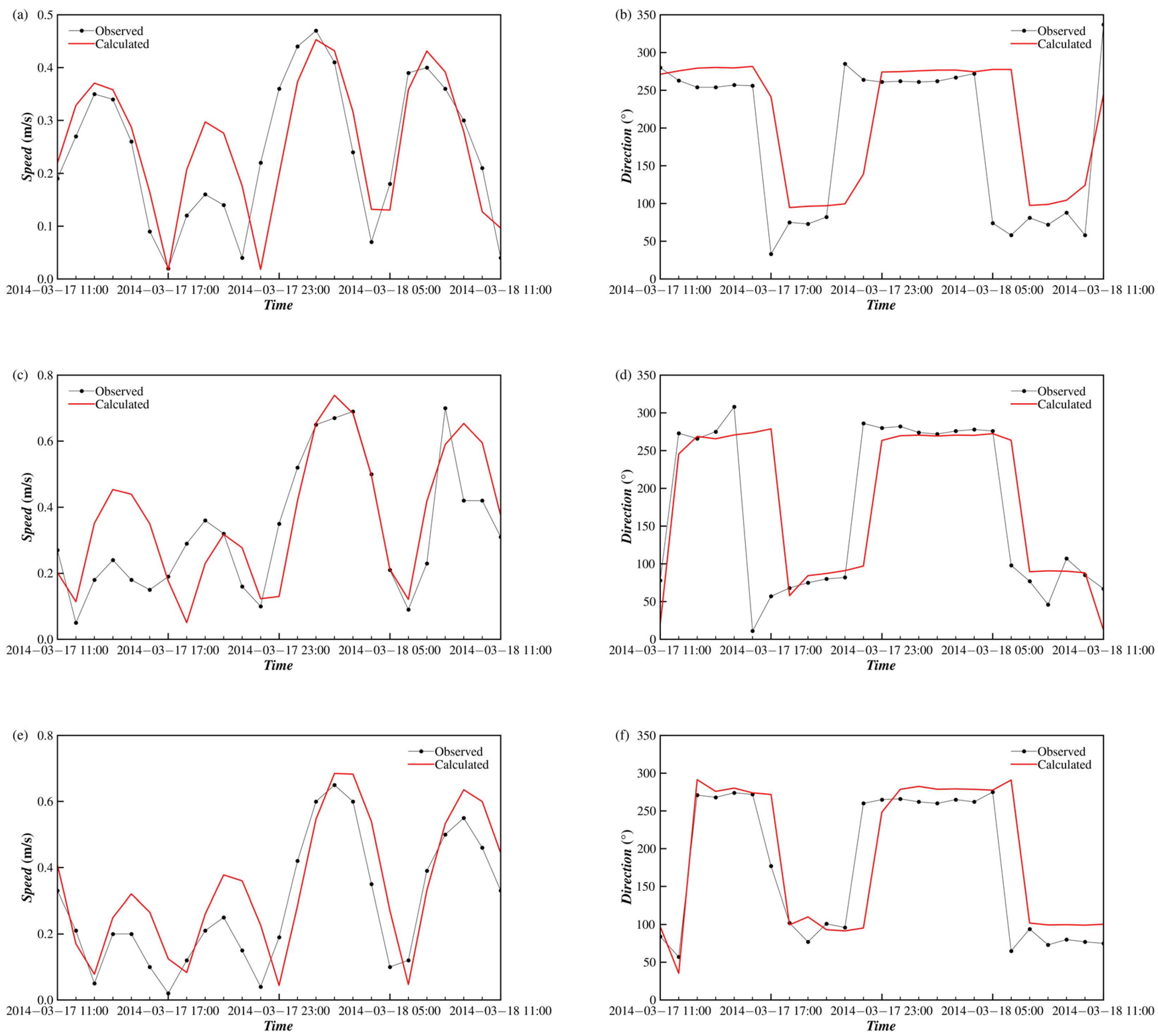
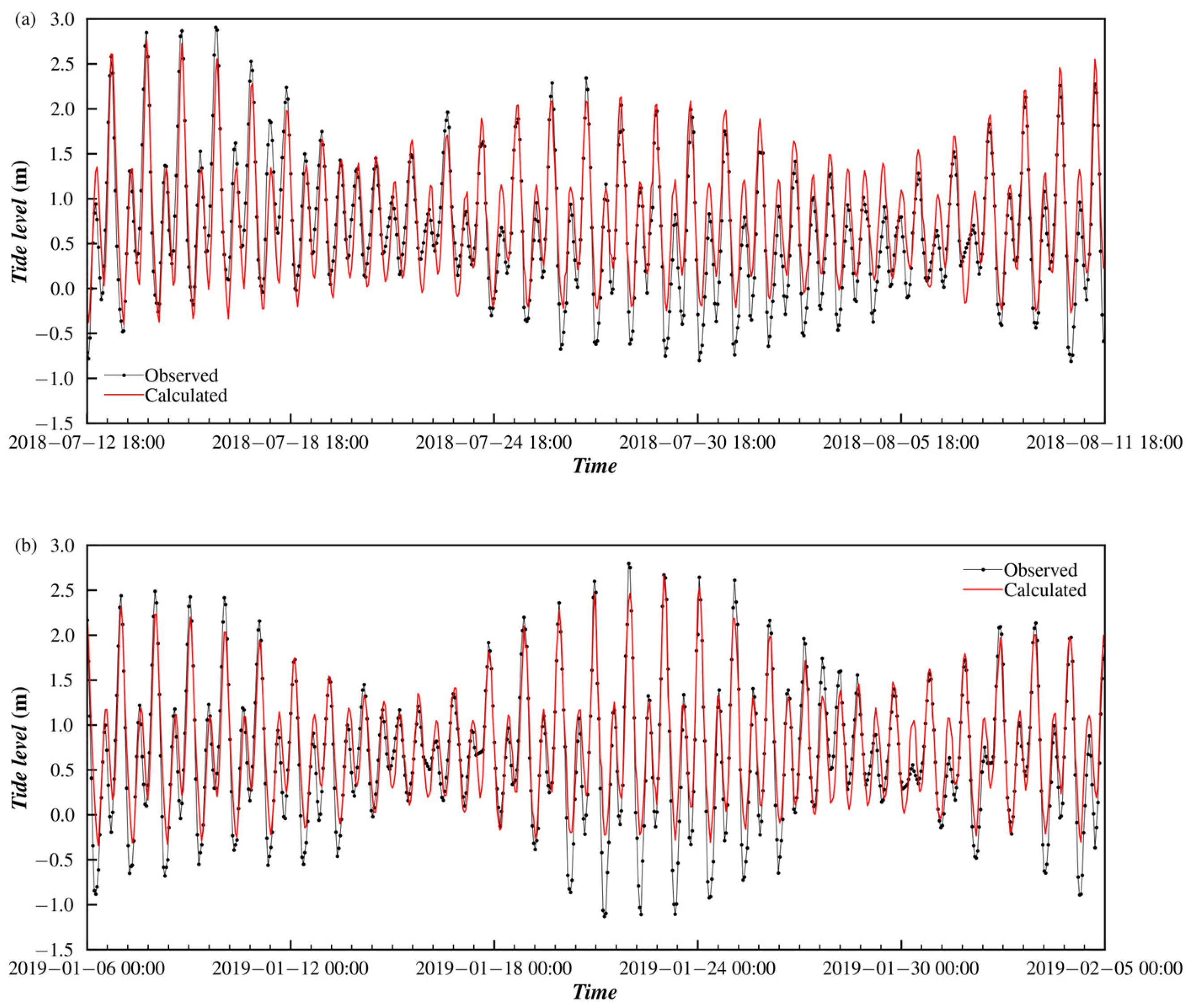
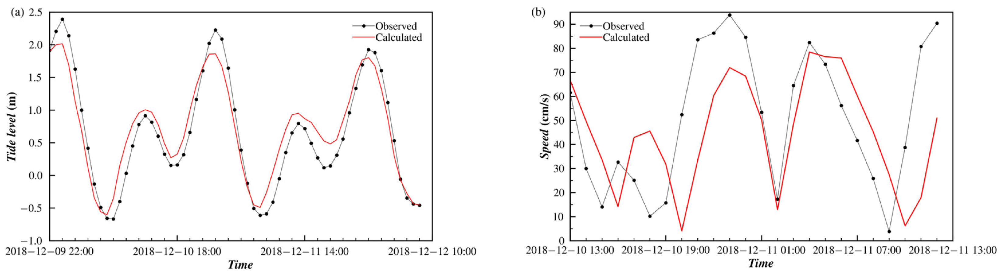
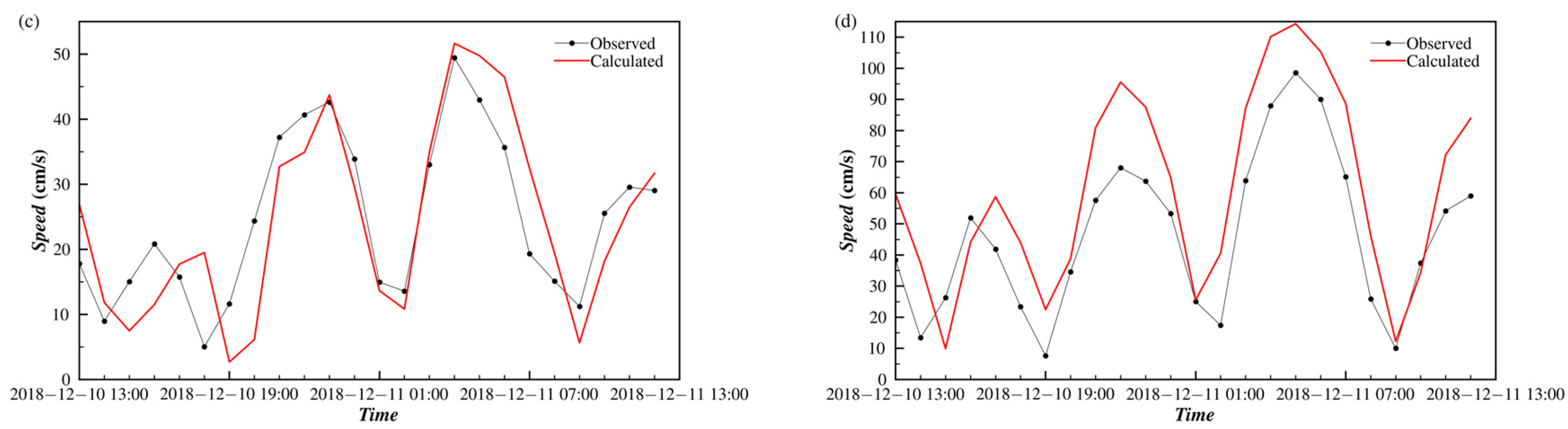
4.2.1. Numerical Results

Figure 11 displays the curves of observed and computed values from long-term observation at the T2 station. The simulation results showed good agreement with observational data during high tide, while some discrepancies were noted during low tide. Nonetheless, the accuracy error remained within 5%, which satisfied the requirements for computational applications. Potential sources of error can be attributed to three main factors: (1) the constant bed friction coefficient used in the model, which significantly affects frictional forces during low tide; (2) the simulation of wetting and drying processes at the T2 station, which is located near the intertidal zone and may introduce errors during low tide; and (3) the lack of measured bathymetry data. Although the 2021 GEBCO bathymetry data were used in this study, they had relatively limited local accuracy, and the time between the calculation period (2018–2019) and the data acquisition time may have had some slight changes in local terrain, thus contributing to simulation deviations. This limitation may have led to deviations in hydrodynamic processes, particularly in shallow water regions during low tide.

4.2.2. Analysis of Tidal Current Characteristics

Figure 12 presents the short-term observed and computed values from four observation stations near Naozhou Island. The tide level and velocity variations calculated by the model aligned with the trends observed in the actual data. Apart from the inherent discretization errors of the model, potential sources of discrepancies could have arisen from the presence of numerous deep troughs in the Zhanjiang area, where frequent adjustments in terrain occur. As a result, differences between the topographical data from GEBCO and current data may have led to errors in extreme flow velocities.
From Figure 12a, it can be observed that the first high tide occurs between midnight and 2:00, while the first low tide happens in the morning between 6:00 and 8:00. The second high tide falls around noon between 12:00 and 14:00, and the second low tide occurs in the afternoon around 18:00, which is consistent with the characteristics of a semi-diurnal tide.
Figure 13 illustrates the flow velocity vector maps at four typical moments in the vicinity of Naozhou Island. In Figure 13a, during the rising tide, seawater flows from the South China Sea into Leizhou Bay on the east side of Naozhou Island, causing a rise in water levels. At this time, the dominant flow direction in the strait near Donghai Island is southwest (SW), while in the southern waters of Naozhou Island, it is northwest (NW). In Figure 13b, during the falling tide, seawater flows from the Leizhou Bay past Naozhou Island towards the South China Sea, leading to a decrease in water levels. The main flow direction in the strait near Donghai Island shifts to northeast (NE), while in the southern waters of Naozhou Island, it becomes southeast (SE). A distinct oscillatory back-and-forth flow occurs between Naozhou Island and Donghai Island, while near the mouth of Leizhou Bay, the flow exhibits a combination of oscillatory and rotational movements. Figure 13c,d are similar to Figure 13a,b and show the distribution of flow velocity vectors during the rising and falling processes of high tides with relatively lower tide levels.
Figure 14 presents the distribution of speed at two typical moments of high tide rising and falling tide in the early morning of 11 December 2018. During high tide, the speed in the vicinity of Naozhou Island is roughly equal. Due to the narrow waterway near Donghai Island, the flow speed is relatively higher, reaching up to 0.8 m/s. The distribution of tidal current intensity during the falling tide differs significantly from that during the rising tide. Apart from the strait near Donghai Island, the flow speed is relatively higher in the southern waters of Naozhou Island and the area adjacent to Leizhou Bay during the falling tide, with the maximum velocity reaching around 1 m/s. The analysis suggests that this is mainly due to the smaller bay area, where the tides are influenced by the tidal wave system in the nearby waters.

5. Conclusions

This study presented the development of a finite element numerical model for tidal currents simulation. This model implemented the finite element method to solve the shallow water equations and incorporated a tidal open boundary condition based on characteristic line theory for tidal current calculations. This approach resulted in a tidal current model that accurately simulates complex boundary conditions.
Based on the SWEs, simulations of the tidal current field were conducted in the Qiongzhou Strait and the region surrounding Naozhou Island. The simulation results demonstrated good agreement with observed data, confirming the accuracy of the developed tidal current model for simulating tidal fields under complex boundary conditions. These validation results suggest the applicability of this model to other coastal regions with similar hydrodynamic characteristics.
Application of the model to the Naozhou Island region revealed that the tides in this area are predominantly semi-diurnal, with minimal spatial variation in tidal range. This characteristic is attributed to the influence of the adjacent tidal wave system and the relatively small size of the bay. During winter, oscillatory flow patterns are observed, with flow directions from southwest to northeast near Donghai Island and from southeast to northwest near Leizhou Bay. Flow speed distribution is generally uniform during high tide, while significantly higher flow speeds occur near the strait adjacent to Donghai Island and Leizhou Bay during low tide. This study provides an important hydrodynamic basis for sustainable utilization of marine resources and related engineering projects in this region.

Author Contributions

Conceptualization and methodology, L.Z.; software, L.Z. and D.P.; validation, L.Z., D.P. and J.M.; investigation, J.L.; resources, J.L.; writing—original draft preparation, D.P.; writing—review and editing, J.M. All authors have read and agreed to the published version of the manuscript.

Funding

The present work is supported by the ‘Postgraduate Research & Practice Innovation Program of Jiangsu Province’ [grant number: KYCX20_0469].

Institutional Review Board Statement

Not applicable.

Informed Consent Statement

Not applicable.

Data Availability Statement

All data generated or analyzed during this study are included in this published article. They are available on request from the corresponding author.

Conflicts of Interest

Jianhua Li is from China Energy Engineering Group Guangdong Electric Power Design Institute Co., Ltd. All the authors declare no conflicts of interest.

References

  1. Egbert, G.D.; Ray, R.D. Significant dissipation of tidal energy in the deep ocean inferred from satellite altimeter data. Nature 2000, 405, 775–778. [Google Scholar] [CrossRef] [PubMed]
  2. Xing, Y.; Shu, C.-W. High-order well-balanced finite difference WENO schemes for a class of hyperbolic systems with source terms. J. Sci. Comput. 2006, 27, 477–494. [Google Scholar] [CrossRef]
  3. Ren, B.F.; Gao, Z.; Gu, Y.G.; Xie, S.S.; Zhang, X.X. A Positivity-Preserving and Well-Balanced High Order Compact Finite Difference Scheme for Shallow Water Equations. Commun. Comput. Phys. 2024, 35, 524–552. [Google Scholar] [CrossRef]
  4. Lukáčová-Medvid’ová, M.; Vlk, Z. Well-balanced finite volume evolution Galerkin methods for the shallow water equations with source terms. Int. J. Numer. Methods Fluids 2005, 47, 1165–1171. [Google Scholar] [CrossRef]
  5. Noelle, S.; Pankratz, N.; Puppo, G.; Natvig, J.R. Well-balanced finite volume schemes of arbitrary order of accuracy for shallow water flows. J. Comput. Phys. 2006, 213, 474–499. [Google Scholar] [CrossRef]
  6. Ern, A.; Piperno, S.; Djadel, K. A well-balanced Runge–Kutta discontinuous Galerkin method for the shallow-water equations with flooding and drying. Int. J. Numer. Methods Fluids 2008, 58, 1–25. [Google Scholar] [CrossRef]
  7. Xing, Y.; Shu, C.-W. High order well-balanced finite volume WENO schemes and discontinuous Galerkin methods for a class of hyperbolic systems with source terms. J. Comput. Phys. 2006, 214, 567–598. [Google Scholar] [CrossRef]
  8. Umgiesser, G.; Canu, D.M.; Cucco, A.; Solidoro, C. A finite element model for the Venice Lagoon. Development, set up, calibration and validation. J. Mar. Syst. 2004, 51, 123–145. [Google Scholar] [CrossRef]
  9. Mandelman, I.; Ferrari, M.A.; Fernández, D.R. Evaluation of a finite element formulation for the shallow water equations with numerical smoothing in the Gulf of San Jorge. Comput. Appl. Math. 2023, 43, 5. [Google Scholar] [CrossRef]
  10. Kawahara, M.; Hirano, H.; Tsubota, K.; Inagaki, K. Selective lumping finite element method for shallow water flow. Int. J. Numer. Methods Fluids 1982, 2, 89–112. [Google Scholar] [CrossRef]
  11. Jiang, C.; Yang, C.; Liang, D. Computation of shallow wakes with the fractional step finite element method. J. Hydraul. Res. 2009, 47, 127–136. [Google Scholar] [CrossRef]
  12. Grotkop, G. Finite element analysis of long-period water waves. Comput. Methods Appl. Mech. Eng. 1973, 2, 147–157. [Google Scholar] [CrossRef]
  13. Mao, J.; Zhao, L.; Bai, X.; Guo, B.; Liu, Z.; Li, T. A novel well-balanced scheme for modeling of dam break flow in drying-wetting areas. Comput. Fluids 2016, 136, 324–330. [Google Scholar] [CrossRef]
  14. Bermudez, A.; Vazquez, M.E. Upwind methods for hyperbolic conservation laws with source terms. Comput. Fluids 1994, 23, 1049–1071. [Google Scholar] [CrossRef]
  15. Kuiry, S.N.; Sen, D.; Ding, Y. A high-resolution shallow water model using unstructured quadrilateral grids. Comput. Fluids 2012, 68, 16–28. [Google Scholar] [CrossRef]
  16. Xing, Y.; Zhang, X.; Shu, C.-W. Positivity-preserving high order well-balanced discontinuous Galerkin methods for the shallow water equations. Adv. Water Resour. 2010, 33, 1476–1493. [Google Scholar] [CrossRef]
  17. Gourgue, O.; Comblen, R.; Lambrechts, J.; Kärnä, T.; Legat, V.; Deleersnijder, E. A flux-limiting wetting–drying method for finite-element shallow-water models, with application to the Scheldt Estuary. Adv. Water Resour. 2009, 32, 1726–1739. [Google Scholar] [CrossRef]
  18. Bunya, S.; Kubatko, E.J.; Westerink, J.J.; Dawson, C. A wetting and drying treatment for the Runge–Kutta discontinuous Galerkin solution to the shallow water equations. Comput. Methods Appl. Mech. Eng. 2009, 198, 1548–1562. [Google Scholar] [CrossRef]
  19. Kärnä, T.; de Brye, B.; Gourgue, O.; Lambrechts, J.; Comblen, R.; Legat, V.; Deleersnijder, E. A fully implicit wetting–drying method for DG-FEM shallow water models, with an application to the Scheldt Estuary. Comput. Methods Appl. Mech. Eng. 2011, 200, 509–524. [Google Scholar] [CrossRef]
  20. Rompas, P.T.D.; ManongkoFaculty, J.D.I. Numerical simulation of marine currents in the Bunaken Strait, North Sulawesi, Indonesia. Iop. Conf. Ser.-Mat. Sci. 2016, 128, 012003. [Google Scholar] [CrossRef]
  21. Barth, A.; Alvera-Azcárate, A.; Beckers, J.M.; Weisberg, R.H.; Vandenbulcke, L.; Lenartz, F.; Rixen, M. Dynamically constrained ensemble perturbations—Application to tides on the West Florida Shelf. Ocean Sci. 2009, 5, 259–270. [Google Scholar] [CrossRef]
  22. Walters, R.A.; Gillibrand, P.A.; Bell, R.G.; Lane, E.M. A study of tides and currents in Cook Strait, New Zealand. Ocean Dyn. 2010, 60, 1559–1580. [Google Scholar] [CrossRef]
  23. Le, H.-A.; Lambrechts, J.; Ortleb, S.; Gratiot, N.; Deleersnijder, E.; Soares-Frazão, S. An implicit wetting–drying algorithm for the discontinuous Galerkin method: Application to the Tonle Sap, Mekong River Basin. Environ. Fluid Mech. 2020, 20, 923–951. [Google Scholar] [CrossRef]
  24. Zhang, Z.; Song, Z.; Zhang, D.; Hu, D.; Yu, Z.; Yue, S. Tide–Surge Interactions in Lingdingyang Bay, Pearl River Estuary, China: A Case Study from Typhoon Mangkhut, 2018. Estuaries Coasts 2024, 47, 330–351. [Google Scholar] [CrossRef]
  25. Hu, P.; Zhao, Z.; Ji, A.; Li, W.; He, Z.; Liu, Q.; Li, Y.; Cao, Z. A GPU-Accelerated and LTS-Based Finite Volume Shallow Water Model. Water 2022, 14, 922. [Google Scholar] [CrossRef]
  26. Chen, Z.R.; Zhang, Q.H.; Ran, G.Q.; Nie, Y. A Wetting and Drying Approach for a Mode-Nonsplit Discontinuous Galerkin Hydrodynamic Model with Application to Laizhou Bay. J. Mar. Sci. Eng. 2024, 12, 147. [Google Scholar] [CrossRef]
  27. Su, M.D.; Xu, X.; Zhu, J.L.; Hon, Y.C. Numerical simulation of tidal bore in Hangzhou Gulf and Qiantangjiang. Int. J. Numer. Methods Fluids 2001, 36, 205–247. [Google Scholar] [CrossRef]
  28. He, A.; He, X.; Bai, Y.; Zhu, Q.; Gong, F.; Huang, H.; Pan, D. Simulation of Sedimentation in Lake Taihu with Geostationary Satellite Ocean Color Data. Remote Sens. 2019, 11, 379. [Google Scholar] [CrossRef]
  29. Zienkiewicz, O.C.; Wu, J. A general explicit or semi-explicit algorithm for compressible and incompressible flows. Int. J. Numer. Meth. Eng. 1992, 35, 457–479. [Google Scholar] [CrossRef]
  30. Chorin, A.J. A numerical method for solving incompressible viscous flow problems (Reprinted from the Journal of Computational Physics, vol 2, pg 12-26, 1997). J. Comput. Phys. 1997, 135, 118–125. [Google Scholar] [CrossRef]
  31. Le Provost, C.; Genco, M.L.; Lyard, F.; Vincent, P.; Canceil, P. Spectroscopy of the world ocean tides from a finite element hydrodynamic model. J. Geophys. Res. Ocean. 1994, 99, 24777–24797. [Google Scholar] [CrossRef]
  32. Shi, M.; Chen, C.; Xu, Q.; Lin, H.; Liu, G.; Wang, H.; Wang, F.; Yan, J. The Role of Qiongzhou Strait in the Seasonal Variation of the South China Sea Circulation. J. Phys. Oceanogr. 2002, 32, 103–121. Available online: https://journals.ametsoc.org/view/journals/phoc/32/1/1520-0485_2002_032_0103_troqsi_2.0.co_2.xml (accessed on 25 January 2025). [CrossRef]
  33. Li, M.; Xie, L.; Zong, X.; Li, J.; Li, M.; Yan, T.; Han, R. Tidal currents in the coastal waters east of Hainan Island in winter. J. Oceanol. Limnol. 2022, 40, 438–455. [Google Scholar] [CrossRef]
  34. Zu, T.; Gan, J.; Erofeeva, S.Y. Numerical study of the tide and tidal dynamics in the South China Sea. Deep-Sea Res. Pt. I 2008, 55, 137–154. [Google Scholar] [CrossRef]
Figure 1. Location of Qiongzhou Strait (from Google Earth).
Sustainability 17 01256 g001
Figure 2. Computational meshes of Qiongzhou Strait.
Sustainability 17 01256 g002
Figure 3. Bathymetrical distribution of Qiongzhou Strait.
Sustainability 17 01256 g003
Figure 4. Tide levels at station W1 by observation and calculation.
Sustainability 17 01256 g004
Figure 5. Comparison of observed and calculated flow speeds and directions during a day of spring tides. (a) The speeds at station V1; (b) the directions at station V1; (c) the speeds at station V2; (d) the directions at station V2; (e) the speeds at station V3; (f) the directions at station V3.
Sustainability 17 01256 g005
Figure 6. Comparison of observed and calculated flow speeds and directions during a day of neap tides. (a) The speeds at station V1; (b) the directions at station V1; (c) the speeds at station V2; (d) the directions at station V2; (e) the speeds at station V3; (f) the directions at station V3.
Sustainability 17 01256 g006
Figure 7. Calculation area of Naozhou Island.
Sustainability 17 01256 g007
Figure 8. Bathymetrical distribution of Naozhou Island.
Sustainability 17 01256 g008
Figure 9. Computational meshes of Naozhou Island.
Sustainability 17 01256 g009
Figure 10. Distribution of observation stations (from Google Earth).
Sustainability 17 01256 g010
Figure 11. Observed and computed values from the T2 station. (a) Tide levels in summer; (b) tide levels in winter.
Sustainability 17 01256 g011
Figure 12. Observed and computed values from short-term stations. (a) The tide levels at station T1; (b) the speeds at station C1; (c) the speeds at station C2; (d) the speeds at station C3.
Sustainability 17 01256 g012aSustainability 17 01256 g012b
Figure 13. Distributions of velocity vectors in the sea around Naozhou island. (a) 2018−12−09 22:00; (b) 2018−12−10 04:00; (c) 2018−12−10 12:00; (d) 2018−12−10 21:00.
Sustainability 17 01256 g013aSustainability 17 01256 g013b
Figure 14. Distributions of speed in the sea around Naozhou Island. (a) 2018−12−10 23:00; (b) 2018−12−11 03:00.
Sustainability 17 01256 g014
Table 1. Observation station coordinates and observation parameters.
StationCoordinatesObservation Parameters and Time
W1109°57.113′ E, 20°15.104′ NTide levelFrom 22 Feb. 16:00 to 24 Mar. 15:00, 2014
V1109°59.064′ E, 20°13.741′ NFlow speed and
direction
Spring tide: From 23 Mar. 11:00 to 24 Mar. 12:00, 2014
Neap tide: From 17 Mar. 11:00 to 24 Mar. 12:00, 2014
V2109°59.142′ E, 20°10.103′ NFlow speed and
direction
V3109°58.829′ E, 20°02.952′ NFlow speed and
direction
Table 2. The coordinates of the tide forecast points for Naozhou Island.
Forecast PointsLongitudeLatitude
I110°31.18′ E20°29.97′ N
J111°14.97′ E20°29.97′ N
K111°14.97′ E21°29.56′ N
Table 3. Observation station coordinates and observation times.
StationCoordinatesTime
T1110°33.000′ E, 20°54.000′ NFrom 22:00 on 9 Dec. 2018, to 09:00 on 12 Dec. 2018
T2110°21.786′ E, 20°49.270′ NSummer: From 18:00 on 12 Jul. 2018, to 23:00 on 11 Aug. 2018
Winner: From 00:00 on 6 Jan. 2019, to 23:00 on 6 Feb. 2109
C1110°32.562′ E, 20°53.819′ NFrom 13:00 on 10 Dec. 2018 to 14:00 on 11 Dec. 2018
C2110°35.434′ E, 20°58.759′ N
C3110°31.450′ E, 20°51.826′ N
Disclaimer/Publisher’s Note: The statements, opinions and data contained in all publications are solely those of the individual author(s) and contributor(s) and not of MDPI and/or the editor(s). MDPI and/or the editor(s) disclaim responsibility for any injury to people or property resulting from any ideas, methods, instructions or products referred to in the content.

