Optimal Land Selection for Agricultural Purposes Using Hybrid Geographic Information System–Fuzzy Analytic Hierarchy Process–Geostatistical Approach in Attur Taluk, India: Synergies and Trade-Offs Among Sustainable Development Goals

Abstract

The precise selection of agricultural land is essential for guaranteeing global food security and sustainable development. Additionally, agricultural land suitability (AgLS) analysis is crucial for tackling issues including resource scarcity, environmental degradation, and rising food demands. This research examines the synergies and trade-offs among the sustainable development goals (SDGs) using a hybrid geographic information system (GIS)–fuzzy analytic hierarchy process (FAHP)–geostatistical framework for AgLS analysis in Attur Taluk, India. The area was chosen for its varied agro-climatic conditions, riverine habitats, and agricultural importance. Accordingly, data from ten topographical, climatic, and soil physiochemical variables, such as slope, temperature, and soil texture, were obtained and analyzed to carry out the study. The geostatistical analysis demonstrated the spatial variability of soil parameters, providing essential insights into key factors in the study area. Based on the receiver operating characteristic curve analysis, the results showed that the FAHP method (AUC = 0.71) outperformed the equal-weighting scheme (AUC = 0.602). Moreover, suitability mapping designated 17.31% of the study area as highly suitable (S1), 41.32% as moderately suitable (S2), and 7.82% as permanently unsuitable (N2). The research identified reinforcing and conflicting correlations with SDGs, emphasizing the need for policies to address trade-offs. The findings showed 40% alignment to climate action (SDG 13) via improved resilience, 33% to clean water (SDG 6) by identifying low-salinity zones, and 50% to zero hunger (SDG 2) through sustainable food systems. Conflicts arose with SDG 13 (20%) due to reliance on rain-fed agriculture, SDG 15 (11%) from soil degradation, and SDG 2 (13%) due to inefficiencies in low-productivity zones. A sustainable action plan (SAP) can tackle these issues by promoting drought-resistant crops, nutrient management, and participatory land-use planning. This study can provide a replicable framework for integrating agriculture with global sustainability objectives worldwide.

1. Introduction

Riverine corridors involve distinctive natural resources, including fertile soils and freshwater, which make them optimal sites for agricultural production and promote worldwide socio-economic growth [1]. The agriculture sector encounters substantial challenges in fulfilling food demands due to a rapidly growing population, inadequate land utilization, and unforeseen climatic variations [2]. These challenges collectively impact food security for roughly 30% of the world’s population [3]. For instance, the green revolution in India attained food grain self-sufficiency but resulted in significant environmental repercussions, including soil fertility depletion, water pollution, and crop diseases [4]. The increasing demands require the identification of appropriate agricultural lands in stressed areas to alleviate food security threats and promote sustainable production systems [5].

Agricultural land suitability (AgLS) analysis has become an essential tool for promoting sustainable agricultural output in developing nations [6]. AgLS systematically assesses the viability of a land area for designated agricultural applications, utilizing classification frameworks such as “highly suitable” and “moderately suitable” to measure suitability based on an amalgamation of environmental, social, and economic variables [7]. Key parameters encompass topographical characteristics, lithological composition, soil physicochemical properties, socio-economic variables, and climatic circumstances, which delineate the potential and constraints for land utilization [8]. These factors are examined in several research studies under diverse climatic settings, highlighting the adaptability and breadth of AgLS analysis globally [9].

Diverse methodologies have been suggested to identify appropriate areas for agricultural use, encompassing both conventional field-based strategies and sophisticated geographic information system (GIS) techniques [10]. Traditional field-based techniques, such as soil sampling and environmental observation, yield accurate local-scale data but are frequently labor-intensive, expensive, and impractical for broader applications [11]. The aforementioned restrictions have prompted the utilization of advanced methodologies such as GIS, which have demonstrated remarkable proficiency in handling geospatial information and assessing land suitability in the context of spatial planning [12]. GIS enables the incorporation of environmental, social, and economic variables into a spatially explicit decision-making framework, providing scalability and accuracy [13]. Moreover, geostatistical methods like semivariogram analysis and kriging are extensively employed to examine the spatial variability of soil characteristics, facilitating the development of prediction maps that delineate significant agricultural areas [14]. Multi-criteria decision analysis (MCDA) approaches, including weighted linear combination (WLC), analytical hierarchy process (AHP), and fuzzy logic modeling, have emerged as effective tools for evaluating land suitability, complementing GIS and geostatistics [15]. AHP organizes decision-making via pairwise comparisons, although its subjective weight assignment frequently constrains accuracy [16]. Fuzzy logic modeling provides more flexibility by employing fuzzy membership functions to address uncertainty in decision-making [17]. The integration of fuzzy logic with AHP, referred to as the fuzzy analytical hierarchy process (FAHP), has augmented the reliability of land suitability evaluations by mitigating inherent ambiguities and refining the accuracy of weighted factor analysis [18]. Studies utilizing GIS-based FAHP have effectively combined soil, climate, and topographical data to generate precise and reliable suitability maps, illustrating the efficacy of this hybrid methodology in facilitating sustainable agricultural planning [19].

The 17 sustainable development goals (SDGs) underscore the necessity of harmonizing economic, environmental, and social aspects in any hydrological system to achieve sustainability [20]. The selection of agricultural land may positively contribute to meeting many SDGs [2]. Challenges emerge from possible conflicts between land use and the objectives of SDGs as agricultural expansion may result in deforestation and soil degradation [4]. Previous research underscored the necessity of integrating the three pillars of sustainability into land-use planning to alleviate such challenges [15]. Promising techniques, such as GIS and MCDA, assist policymakers in assuring sustainable agricultural development following the SDGs [17].

More studies are required to analyze synergies and trade-offs between AgLS and SDGs [20,21]. This research provides a unique approach by determining the contribution percentage of delineating AgLS to achieve SDGs target based on either reinforcing or conflicting linkages. Using a proposed GIS-FAHP–geostatistical approach, the study integrated 10 critical factors encompassing surface (topography and climate) and subsurface (soil physical and chemical properties) of agricultural land to identify reinforcing and conflicting linkages between AgLS and SDGs, offering a novel framework for sustainable agricultural planning. This research focused on Attur Taluk, India, which was selected for its agro-climatic conditions and significant agricultural potential. The primary objectives of this study were to (a) delineate agricultural suitability zones through the proposed GIS-FAHP–geostatistical approach, (b) quantify the synergies and trade-offs between AgLS and key SDG targets, and (c) propose a sustainable action plan (SAP) to mitigate trade-offs and enhance synergies. The proposed methodology can offer significant potential for enhancing long-term agricultural sustainability in urban riverine ecosystems and can serve as a model for addressing similar challenges in other regions worldwide.

2. Materials and Methods

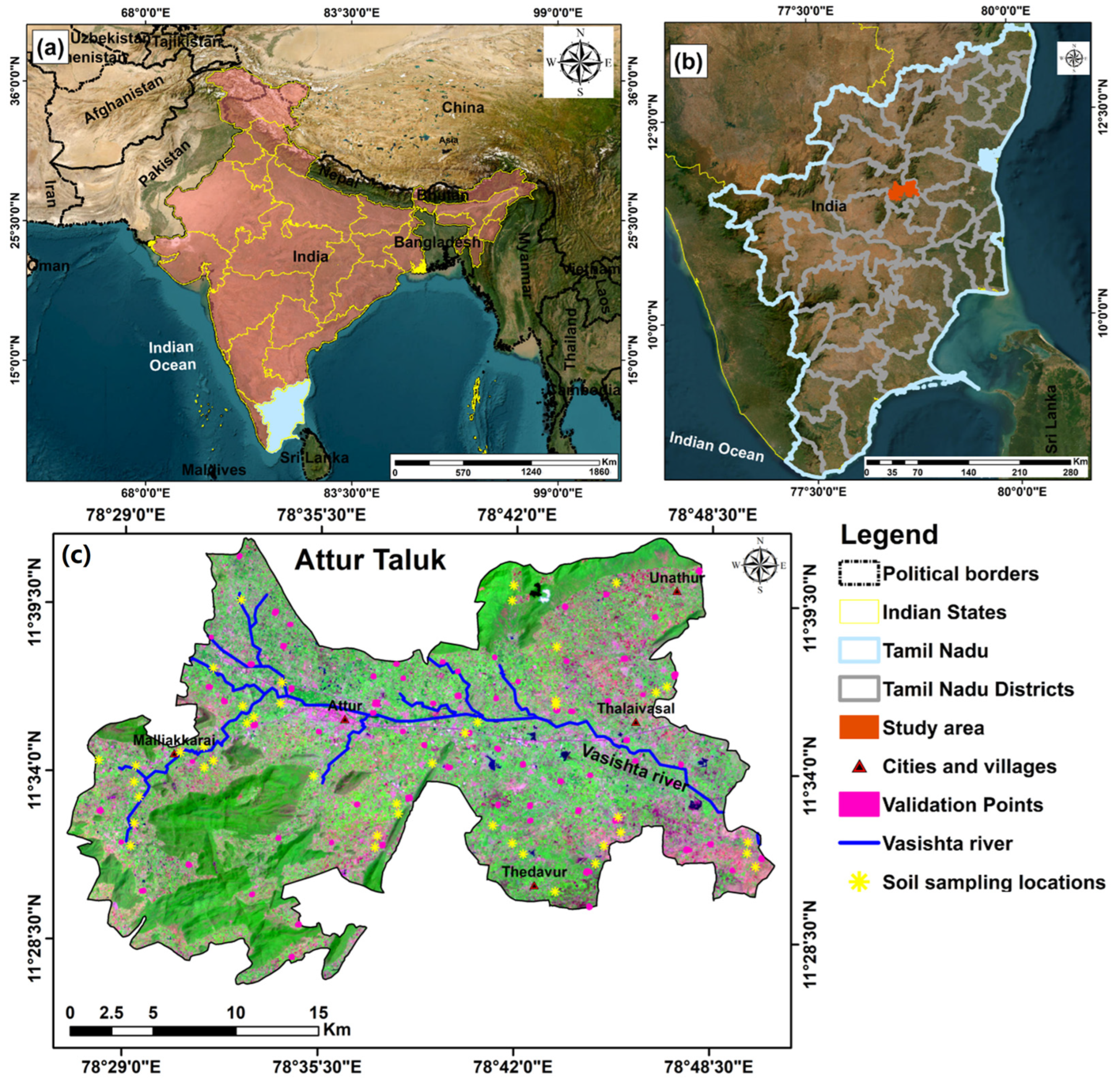
2.1. Study Area

This research was carried out in Attur Taluk, one of the nine taluks in the Salem district of India (Figure 1). Attur Taluk, located in the western region of Tamil Nadu, encompasses an area of 625.13 km². In addition, it is situated between 11.45° and 11.69° N (latitude) and between 78.45° and 78.84° E (longitude). It includes the Vasishta River, a tributary of the Vellar River, which originates in the Chitteri Hills. The Vasishta River runs southeastward into the Bay of Bengal, where it converges with the Vellar River.

Attur, a town recognized for its agricultural output, ranks among the four principal producers of cotton seeds in India [22]. The primary agricultural products in Attur include rice, maize, cotton, tapioca, areca nut, fodder sorghum, coleus, and vegetables such as okra and tomato. The rice mills provide rice nationwide, considerably adding to India’s overall agricultural output [23]. Six unique geomorphic units are recognized within the study area: plateau, structural hills, valley fill, pediments, shallow pediments, and buried pediments [24]. The region consists of granite gneiss, charnockite, granites, and other associated rock formations [25]. The research area exhibits a tropical environment characterized by distinct monsoons. The southwest and northeast monsoons influence the region’s yearly precipitation, which varies from 750 to 1200 mm, with the northeast monsoon as the primary source. The yearly average maximum and minimum temperatures are 34 °C and 17 °C, respectively.

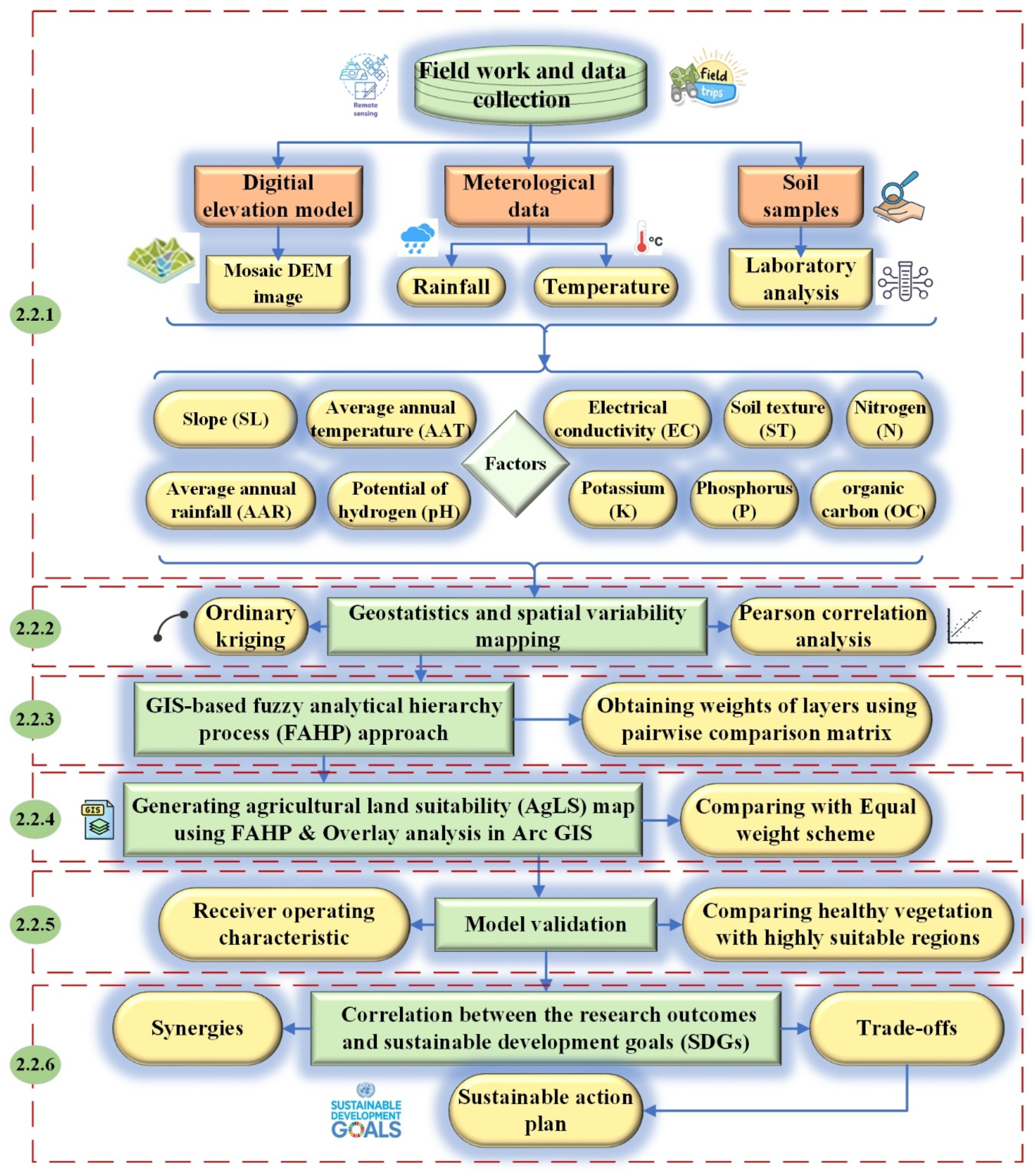
2.2. Datasets and Methodology

This study utilized several data sources to provide a thorough framework for assessing possible AgLS sites in the Attur region. A systematic methodology was employed inside the GIS framework to accomplish the research objectives, which encompassed the following steps (Figure 2):

2.2.1. Fieldwork and Data Preparation

Multi-criteria evaluation entails a systematic methodology within GIS for integrating various input data layers (factors) via informed assessments [26,27,28]. Consequently, ten criteria affecting AgLS were identified for the study area: slope (SL), soil texture (ST), potential of hydrogen (pH), electrical conductivity (EC), organic carbon (OC), available nitrogen (AN), available phosphorus (AP), and available potassium (AK), along with average annual rainfall (AAR) and average annual temperature (AAT), following previous studies [29,30]. The Attur GIS database was developed utilizing publicly accessible resources, comprising satellite Shuttle Radar Topography Mission (SRTM) images and global climate data from the Climate Forecast System Reanalysis (CFSR), in conjunction with field soil sampling measures, as illustrated in the following sections.

• Topographical Elements

This research employed SRTM–Digital Elevation Model (SRTM-DEM) data. The SRTM-DEM was acquired via the United States Geological Survey (USGS) website [29] at a resolution of 30 m. The spatial distribution of SL was obtained from a mosaic DEM image utilizing GIS 10.8.

• Climatic Variables

Daily precipitation and temperature data from 2000 to 2015 were acquired from the worldwide CFSR product [30] in the Soil and Water Assessment Tool (SWAT) format. CFSR is a comprehensive, high-resolution system encompassing atmospheric, oceanic, land surface, and sea ice data, aimed at providing the most precise information for the obtained period [31]. The yearly average climatic datasets for temperature (minimum and maximum) and AAR were interpolated.

• Soil Physicochemical Factors

During fieldwork, 85 random soil samples were obtained from the study region (Figure 1). Sampling locations were specified utilizing a global positing system (GPS) device (Garmin GPS Map 76CSx, Garmin Ltd., Lenexa, KS, USA) in collaboration with farm proprietors knowledgeable about their terrain. The sampling strategy adhered to the protocols set forth by Tamil Nadu Agricultural University [32]. Soil samples, both disturbed and undisturbed, were obtained at a depth of 0–15 cm. Intact samples were collected with a core sampler for the study of bulk density. Disturbed samples were gathered in a V-formation using a spade and subsequently air-dried before filtering through a 2 mm mesh. All samples were preserved in airtight containers for subsequent laboratory analyses, which included soil pH determined by the pH meter method [33], soil EC assessed via the conductometric method [33], soil particle size distribution (sand, silt, and clay) measured using the Bouyoucos hydrometer method [34], soil OC quantified through the wet oxidation method [35], AN evaluated by the alkaline potassium permanganate method [36], AP determined by the Olsen method [37], and AK measured using the normal neutral ammonium acetate method [38].

2.2.2. Geostatistics and Spatial Variability Mapping

A geostatistical analysis is a method for examining spatial variability, derived from classical statistics [39]. Two statistical methods, Pearson correlation analysis and ordinary kriging, were utilized. In addition, descriptive statistics are efficient instruments that yield valuable insights into soil factors. The descriptive statistics for the variables were computed utilizing the data analysis add-in of Microsoft Excel. Then, the Pearson correlation coefficient (r) was calculated to assess the correlations among the soil properties.

Geospatial mapping requires the utilization of a theoretical semivariogram to forecast spatial variations at unsampled sites. A semivariogram is a graphical instrument that illustrates the geographical dependency of a soil attribute, demonstrating how the variance between samples varies with increasing distance of separation. The semivariogram $\mathsf{\gamma }\left(\mathrm{h}\right)$ can be calculated using Equation (1) [40].

$$\mathsf{\gamma }\left(\mathrm{h}\right)={\displaystyle \frac{1}{2\mathrm{N}\left(\mathrm{h}\right)}}{\sum }_{i,j\in h}^{\mathrm{N}\left(\mathrm{h}\right)}{\left(\mathrm{Z}\left({\mathrm{x}}_{\mathrm{i}}\right)-\mathrm{Z}({\mathrm{x}}_{\mathrm{j}})\right)}^2$$

(1)

where N(h) denotes the number of pairings distanced by (h), whereas Z(x_i) and Z(x_j) signify the values of the variable (Z) at positions (x_i) and (x_j), respectively.

This study utilized multiple semivariogram models, specifically the Gaussian, spherical, and exponential models, to determine the model that most accurately represents the spatial distribution of each soil attribute. Models with the lowest root mean square error (RMSE) were chosen for subsequent investigation, signifying a superior alignment between the predicted and actual values of soil characteristics. RMSE can be estimated using Equation (2) at (n) locations [16].

$$\mathrm{R}\mathrm{M}\mathrm{S}\mathrm{E}=\sqrt{{\displaystyle \frac{1}{\mathrm{n}}}{\sum }_{\mathrm{i}=1}^{\mathrm{n}}{(\mathrm{a}\mathrm{c}\mathrm{t}\mathrm{u}\mathrm{a}\mathrm{l} \mathrm{v}\mathrm{a}\mathrm{l}\mathrm{u}\mathrm{e}-\mathrm{p}\mathrm{r}\mathrm{e}\mathrm{d}\mathrm{i}\mathrm{c}\mathrm{t}\mathrm{e}\mathrm{d} \mathrm{v}\mathrm{a}\mathrm{l}\mathrm{u}\mathrm{e})}^2}$$

(2)

The interpolation of soil parameters was subsequently conducted using the ordinary kriging technique, employing the most suitable semivariogram model. Ordinary kriging was selected for the generation of attribute data layers because of its numerous advantages. It adeptly mitigates the constraints of low sample density by employing the optimal semivariogram model, in contrast to more rudimentary interpolation techniques. In addition, it provides a probabilistic assessment of interpolation accuracy (uncertainty), as articulated by Burrough and McDonnell [41]. Moreover, it utilizes spatial correlations to compute a target variable Z at a specified point X₀, employing a series of values of the same parameter obtained at (n) locations near the estimate points X_i (Equation (3)) [42].

$$\mathrm{Z}\left({\mathrm{X}}_0\right)={\mathrm{a}}_0+{\sum }_{\mathrm{i}=1}^{\mathrm{n}}{\mathsf{\lambda }}_{\mathrm{i}}\mathrm{Z}\left({\mathrm{x}}_{\mathrm{i}}\right)$$

(3)

where ${\mathrm{a}}_0$ = constant, and ${\mathsf{\lambda }}_{\mathrm{i}}$ = weighting factor.

Ordinary kriging was utilized to obtain skewed estimations, deliberately minimizing low values and exaggerating high values. This was achieved by applying a spatial variability model to the sample data, to minimize errors in the resultant soil physiochemical maps relative to the provided datasets. The model’s accuracy was ultimately evaluated via cross-validation, and calculating the RMSE between observed and predicted values.

2.2.3. Geographic Information System (GIS)-Based Fuzzy Analytical Hierarchy Process (FAHP) Approach

FAHP is a decision-making methodology that uses fuzzy numbers to evaluate and contrast various criteria. The development of the FAHP technique was driven by the necessity to resolve the widespread problem of ambiguity in decision-making contexts [43]. A triangular fuzzy number (TFN) is a mathematical construct that measures the relative magnitude of each component pair within a specified hierarchy. M can be represented as M = (l, m, u), where l denotes the lower bound, m signifies the median, and u represents the upper bound, adhering to the TFN constraint l < m < u in a fuzzy event [17]. When l = m = u, it is considered a non-fuzzy number by convention. The triangle membership function (TMF) can be employed to delineate a set by allocating a membership grade between zero and one to each element. A fuzzy set (A) can be defined using Equations (4) and (5) [44].

A = {x, µA (x)}x ∈ X

(4)

$$\mathrm{A}\left(\mathrm{x}\right)=\left\{\begin{array}{c}{\displaystyle \frac{\mathrm{x}-\mathrm{l}}{\mathrm{m}-\mathrm{l}}}, \mathrm{l}\le \mathrm{x}\le \mathrm{m}\\ {\displaystyle \frac{\mathrm{u}-\mathrm{x}}{\mathrm{u}-\mathrm{m}}}, \mathrm{l}\le \mathrm{x}\le \mathrm{m}\\ 0, \mathrm{other} \mathrm{wise}\end{array}\right.$$

(5)

where X = {x} is a finite set of points, and µA(x) is a membership function of x in A.

The following steps were employed for AgLS in Attur, India, using the FAHP method:

• Step (1)

A fuzzification pairwise comparison matrix (PWCM) is created utilizing the TFN associated with each variable, determined by the relative importance scale established by Saaty [16]. The TMF was utilized for the development of the PWCM (Table S2). In the FAHP method, factors were ranked from 1 to 9 based on the fundamental scale established by Saaty [16]. The exact weight rankings were subsequently fuzzificated and categorized into upper, middle, and lower weight classifications. In FAHP, PWCM and TFN can be articulated using Equations (6)–(8) [8].

A = (ãij)n × n = [(1,1,1)(l12, m12, u12)…(l1n, m1n, u1n)(l21, m21, u22)

(6)

(1,1,1)…(l2n, m2n, u2n)⋮⋮⋮(ln1, mn1, un1)

(7)

(ln2, mn2, un2)…(1,1,1)

(8)

where ãij = (lij, mij, uij), ãij − 1 = (1/uij, 1/mij, lij), i,j = 1,…, n, and i ≠ j.

The crisp numeric value was fuzzified as $ℳ$A(x) = A = (l,m,u) and further reciprocated by Equation (9).

A⁻¹ = (l, m, u)⁻¹ = (1u, 1m, 1l)

(9)

• Step (2)

The geometric mean was utilized to calculate a fuzzy weight (wi) for the ten thematic data layers [45]. The geometric mean was computed using Equation (10).

A1 × A2 = (l1, m1, u1) × (l2, m2, u2) = (l1 × l2, m1 × m2, u1 × u2)

(10)

• Step (3)

Subsequently, the fuzzy geometric mean was employed to determine the (wi), utilizing Equation (11).

A1 + A2 = (l1, m1, u1) + (l2, m2, u2) = ((l1 + l2), (m1 + m2), (u1 + u2))

(11)

This value was multiplied by the reciprocal of the sum of the geometric mean. Accordingly, this value represented the (wi), as indicated in Table S3.

• Step (4)

To guarantee consistency of estimation, the consistency index (CI) and consistency ratio (CR) were calculated [17]. This method used a random index table to detect any overestimation or underestimation of suitability scores. A CR below 0.1 was deemed acceptable.

• Step (5)

The defuzzification employed weights for each requirement. This study employs the center of area (COA) approach for defuzzification. Equation (12) was employed to compute the defuzzification weight of the centroid value.

COA = wi

(12)

• Step (6)

The normalized weight (Nwi) for each criterion was subsequently calculated using Equation (13):

Nwi = Wi/ΣWjni = 1, J = 1………n

(13)

where ΣNwi = 1, and (i = 1………n).

2.2.4. Generating Agricultural Land Suitability (AgLS) Maps

The study of land suitability depends on the amalgamation of diverse thematic layers/factors within a GIS framework. GIS modeling utilizes two fundamental components for efficient factor analysis: ranking and weighting [17]. The choice of a decision rule is essential since it determines the weighting method employed to consolidate the effects of several factors, and influences the result [46]. This research examined two decision rules in the appropriateness assessment: equal weights and FAHP. Additionally, it provided a concise overview of the procedures for generating AgLS maps with the spatial data modeler extension in GIS 10.8 using the following steps in Attur Taluk, India.

• Step (1)

All input variables were standardized to provide spatial consistency [47]. This entailed transforming each variable into a 30 m resolution raster layer and co-registering them to a unified Universal Transverse Mercator (UTM) projection (WGS84, zone 44N) utilizing ArcMap 10.8.

• Step (2)

The thematic layers were organized with numerical values ranging from five (indicating the highest suitability) to one (designated as permanently unsuited), following criteria from literature reviews [7], field investigations, and further recommendations.

• Step (3)

The predictive AgLS map utilizing the equal weighting scheme (AgLS_Eq) was generated by attributing uniform significance to all assessed elements and analyzing the cumulative intersection for each category through arithmetic overlay, employing Equation (14) [48].

$${\mathrm{AgLS}}_{\mathrm{Eq}}={\sum }_{\mathrm{i}=1}^{{\mathrm{n}}_{\mathrm{f}}}\mathrm{N}\mathrm{w}\mathrm{i}\times {\mathrm{X}}_{\mathrm{i}\mathrm{j}}$$

(14)

where $\mathrm{N}\mathrm{w}\mathrm{i}$ is the weight value of the factor (i),${\mathrm{X}}_{\mathrm{i}\mathrm{j}}$ is the score of the class (j) for the factor (i), and n_f is the number of factors.

• Step (4)

The proposed AgLS map through FAHP (AgLS_FAHP) was produced by multiplying the scored factors by their normalized weight from FAHP (Table S3). The resulting products were then summed to produce the final suitability map using Equation (15) [17].

$${\mathrm{AgLS}}_{\mathrm{FAHP}}={\sum }_{\mathrm{i}=1}^{{\mathrm{n}}_{\mathrm{f}}}\mathrm{N}\mathrm{w}\mathrm{i}\times {\mathrm{X}}_{\mathrm{i}\mathrm{j}}$$

(15)

• Step (5)

The resulting maps were categorized into five suitability classes [49], i.e., highly suitable (S1), moderately suitable (S2), marginally suitable (S3), currently unsuitable (N1), and permanently unsuitable (N2), to identify different zones in the study area.

2.2.5. Model Validation

Modeling site appropriateness without validation lacks scientific significance [50]. The precision of susceptibility models in this study was assessed using the receiver operating characteristic (ROC) curve and basic overlay techniques. The area under the curve (AUC) of ROC, ranging from 0.5 to 1.0, serves as a composite measure of model accuracy for suitability/susceptibility [51]. Elevated AUC values signified superior model performance, classified as outstanding (0.90–1.00), very good (0.80–0.90), good (0.70–0.80), and average (0.60–0.70). AUC can be estimated using Equation (16) [24].

$$\mathrm{A}\mathrm{U}\mathrm{C}=\int \mathrm{T}\mathrm{R}\mathrm{P}\mathrm{d}\left(\mathrm{F}\mathrm{P}\mathrm{R}\right)={\displaystyle \frac{\sum \left[\mathrm{T}\mathrm{R}\mathrm{P}\left(\mathrm{i}+1\right)+\mathrm{T}\mathrm{R}\mathrm{P}\left(\mathrm{i}\right)\right]}{2}}\times \left(\mathrm{F}\mathrm{P}\mathrm{R}\left(\mathrm{i}+1\right)-\mathrm{F}\mathrm{P}\mathrm{R}\left(\mathrm{i}\right)\right)$$

(16)

where TPR is the true positive rate, FPR is the false positive rate, and FPR (i) and TPR (i) are FPR and TPR at the i-th threshold, respectively.

The ROC curve was constructed by correlating the cumulative percentage of areas across various suitability categories with the cumulative count of existing healthy vegetation lands within each suitable class. Additionally, the second validation stage evaluated the concordance between the spatial distribution of current healthy vegetation and the regions designated as moderately to highly appropriate for agriculture. A random sample of 75 farmers was chosen to identify their highest productive field.

2.2.6. Correlation of Research Outcomes to Sustainable Development Goals (SDGs)

The relationship between AgLS outcomes and SDGs was analyzed by linking suitability results from the GIS-FAHP–geostatistical model with relevant SDG targets. This approach cross-referenced land-use suitability layers with the environmental, social, and economic aspects of the SDGs to highlight synergies and trade-offs. This structured methodology can provide a basis for integrating agricultural planning with sustainability objectives, as recommended in prior studies [21].

3. Results and Discussion

3.1. Geostatistics and Spatial Variability of Soil Properties

Agroecosystems exhibit considerable regional heterogeneity in natural soil properties, even within distinct soil strata [52]. Therefore, clarifying the geographical distribution of soil characteristics across these strata is essential for enhancing agricultural field management strategies.

Table 1. Descriptive statistics of soil parameters of Attur Taluk, India.

Soil Parameter	Min.	Max.	Mean	SD	CV	Skewness	Kurtosis
pH	6.20	7.54	6.92	0.28	4.05	−0.47	0.07
EC (dSm−1)	0.12	1.24	0.46	0.29	63.04	1.13	0.44
Sand (%)	32.30	70.30	59.72	6.87	35.29	−1.43	2.50
Silt (%)	2.00	12.00	6.01	2.30	19.63	0.48	−0.36
Clay (%)	25.70	51.20	33.86	5.07	54.96	1.26	1.61
OC	3.40	20.0	10.2	3.6	56.59	0.60	−0.32
AN (kg ha−1)	190.40	420.00	296.31	58.18	33.27	0.19	−0.59
AP (kg ha−1)	10.40	88.30	39.68	21.81	43.08	0.64	−0.57
AK (kg ha−1)	53.70	887.50	231.45	130.97	59.94	1.80	6.27

Note: Min. = minimum; Max. = maximum; SD = standard deviation; CV = coefficient of variation; pH = potential of hydrogen; EC = electrical conductivity; OC = organic carbon; AN = available nitrogen; AP = available phosphorus; AK = available potassium.

displays descriptive statistics regarding the physicochemical characteristics of the soils of Attur Taluk, India. The examination of soil profiles disclosed mean values ranging from 0.46 to 296.31 for the assessed variables. AN, AK, AP, sand, and clay demonstrated elevated mean values (>33.86), whereas the other characteristics showed diminished mean values (<33.86). Soil property variability was classified according to the coefficient of variation (CV) values into low (≤15%), medium (15–35%), and high (≥35%) categories throughout the region [53]. The CV data indicated little variability for soil pH (CV = 4.05%), moderate variability for silt (CV = 19.63%) and AN (CV = 33.27%), and substantial variability for the other characteristics (ranging from 35.29% to 63.04%). Since OC is a relatively recalcitrant component of the soil environment, it demonstrates inherent stability. Nonetheless, its geographical variability may be affected by the severity of pedogenic processes [52]. This observation might be attributed to various contributing elements, including uniform parent material, micro-topography, macro-climate, and effective fertilizer management [54]. Soil chemical content (AK, AN, and AP) showed the highest diversity and the greatest standard deviation (SD) values, followed by ST and OC, respectively, which indicated a broader dispersion of data points for the chemical elements. The kurtosis values for all soil characteristics varied between −0.59 and 6.27 (Table 1). Following the skewness study, the observations for silt, OC, AN, and AP exhibited a nearly symmetrical distribution. In contrast, sand and pH data indicated a leftward skew, whilst EC, clay content, and AK measurements demonstrated a rightward skew, indicating departures from a normal distribution [55]. The significant variety in soil properties was likely due to a combination of anthropogenic and natural influences [17]. Potential influences encompassed agricultural management approaches, intrinsic soil characteristics, and existing climate conditions [56].

Table 2. Correlation of soil parameters based on Pearson correlation coefficient (r) of Attur Taluk, India.

Soil Parameters	pH	EC	OC	AN	AP	AK	Sand	Silt	Clay
pH	1
EC	−0.125	1
OC	0.199	0.080	1
AN	−0.147	0.226 *	0.136	1
AP	−0.261 *	0.173	−0.010	0.192	1
AK	0.139	0.054	0.225 *	0.133	0.203	1
Sand	−0.240 *	−0.035	−0.338 **	−0.060	0.156	−0.373 **	1
Silt	0.205	−0.026	0.319 **	0.028	−0.148	0.334 **	−0.533 **	1
Clay	0.187	−0.064	0.227 *	0.103	−0.194	0.267 *	−0.840 **	0.336 **	1

Note: * is an indication for p-value < 0.05; ** is an indication for p-value < 0.01; pH = potential of hydrogen; EC = electrical conductivity; OC = organic carbon; AN = available nitrogen; AP = available phosphorus; AK = available potassium.

displays the (r) values for the nine soil metrics, examined in Attur Taluk, India. Positive correlations signify the spatial co-occurrence of certain factors, whilst negative correlations imply opposing spatial distribution patterns [57]. pH had a negative correlation with AP (r = −0.261 *) and sand (r = −0.240 *) while demonstrating a positive correlation with silt (r = 0.205). EC had a positive correlation with AN (r = 0.226 *). OC exhibited a positive correlation with silt (r = 0.319 **) and a negative correlation with sand (r = −0.338 **). AP exhibited a favorable correlation with AK (r = 0.203 **). AK had positive associations with silt (r = 0.334 **) and clay (r = 0.267 **) while demonstrating a negative connection with sand (r = −0.373 **). Sand demonstrated substantial negative relationships with silt (r = −0.533 *) and clay (r = −0.840 *). Silt was favorably linked with clay (r = 0.336 **). These data indicated that deliberately reducing pH and sand content in regions with low nutrient levels might substantially enhance the availability of AP, AK, and AN [14].

Multiple semivariogram models, such as spherical, circular, tetraspherical, pentaspherical, rational quadratic, exponential, Gaussian, J-Bessel, and stable, were applied to each dataset. The most suitable semivariogram model for each dataset was selected according to the lowest associated RMSE value (

Table 3. Statistics for different semivariogram models of Attur Taluk, India.

Soil Parameters	Model	Nugget	Partial Sill	Range	Sill	Nugget/Sill Ratio	RMSE	Spatial Dependence
pH	Exponential	0.0446	0.411	5898	0.456	0.098	0.95	Strong
EC	Gaussian	0.0206	0.107	1767	0.128	0.161	1.01	Strong
Sand	Exponential	9.8	36.52	1131	46.320	0.212	1.02	Strong
Silt	Spherical	3.92	2.03	16,875	5.950	0.659	1.02	Moderate
Clay	Spherical	0.25	0.493	24,033	0.743	0.336	0.99	Moderate
OC	Spherical	0.003	0.005	3246	0.008	0.375	1.09	Moderate
AN	Exponential	2464	1128	12,172	3592.000	0.686	1.03	Moderate
AP	Exponential	31	517.65	2145	548.650	0.057	1.01	Strong
AK	Exponential	5880	13,889	1131	19,769.000	0.297	0.94	Moderate

Note: pH = potential of hydrogen; EC = electrical conductivity; OC = organic carbon; AN = available nitrogen; AP = available phosphorus; AK = available potassium; RMSE = root mean square error.

). The exponential model yielded the optimal fit for the datasets of pH, sand, AN, AP, and AK. EC was optimally represented by the Gaussian model. The spherical model was the most appropriate for datasets of silt, clay, and organic carbon. The RMSE values varied from 0.94 to 1.09, signifying a strong correlation between the selected models and the empirical semivariograms. The soil parameters examined in this study exhibited varied spatial dependence as a result of their nugget-to-sill ratios. pH, EC, sand, and AP exhibited considerable spatial dependence, while silt, clay, organic carbon, AN, and AK demonstrated moderate spatial dependence. Robust spatial dependence is mostly linked to intrinsic soil characteristics, including mineralogy and texture. In contrast, considerable spatial dependence indicates the impact of both intrinsic and external variables such as fertilization and plowing [58]. This claim indicated that these models were suitable for predicting and mapping the spatial patterns of the examined soil properties in Attur Taluk, India.

3.2. Contribution of Thematic Layers for Agriculture Suitability

This study utilized 10 thematic layers, including topographic (Figure 3), meteorological (Figure 4), and soil physicochemical characteristics (Figure 5 and Figure 6), to determine optimal sites for AgLS evaluation. The classifications, selection criteria, and intrinsic spatial heterogeneity within Attur Taluk for these thematic layers were elaborated upon (refer to Figure 7 and

Table 4. Weights of all criteria used in the current research of Attur Taluk, India.

Influencing Factor	Class	Class Weight	Factor Weight	Class Weight × Factor Weight
AAT (°C)	22–26	4	0.224	0.896
	18–22 or 26–32	3		0.672
	14–18 or 33–15	2		0.448
	<14 or >35	1		0.224
AAR (mm)	<800	1	0.191	0.191
	800–1200	2		0.382
	<1200	3		0.573
SL (%)	Level (0–1)	6	0.160	0.8
	Very gentle SL (1–3)	5		0.8
	Gentle SL (3–8)	4		0.64
	Moderate SL (8–15)	3		0.48
	Strong SL (15–30)	2		0.32
	Steep SL (>30)	1		0.16
ST	Sandy clay loam	4	0.047	0.188
	Sandy clay	3		0.141
	Clay	2		0.094
	Sandy	1		0.047
pH	Acidic soil (<6.5)	2	0.102	0.204
	Neutral (<6.5–7.5)	3		0.306
	Saline soil (7.5–8.5)	2		0.204
	Alkaline soil (>8.5)	1		0.16
EC (dS m−1)	No restriction (<1)	3	0.095	0.285
	Restriction with some crops (1–4)	2		0.19
	Restricted with all crops (>4)	1		0.095
OC (Kg ha−1)	Low (<5.0)	1	0.062	0.062
	Medium (5.0–7.5)	2		0.124
	High (>7.5)	3		0.186
AN (Kg ha−1)	Low (<280)	1	0.049	0.049
	Medium (280−450)	2		0.098
	High (>450)	3		0.147
AP (Kg ha−1)	Low (<11)	1	0.037	0.037
	Medium (11–22)	2		0.074
	High (>22)	3		0.111
AK (Kg ha−1)	Low (<118)	1	0.034	0.034
	Medium (118−280)	2		0.068
	High (>280)	3		0.102

Note: AAR = average annual rainfall; AAT = average annual temperature; SL = slope; ST = soil texture; pH = potential of hydrogen; EC = electrical conductivity; OC = organic carbon; AN = available nitrogen; AP = available phosphorus; AK = available potassium.

). Table S1 displays the area corresponding to each factor for every appropriateness class. The following section details the outcomes of various thematic layers in delineating AgLS zones.

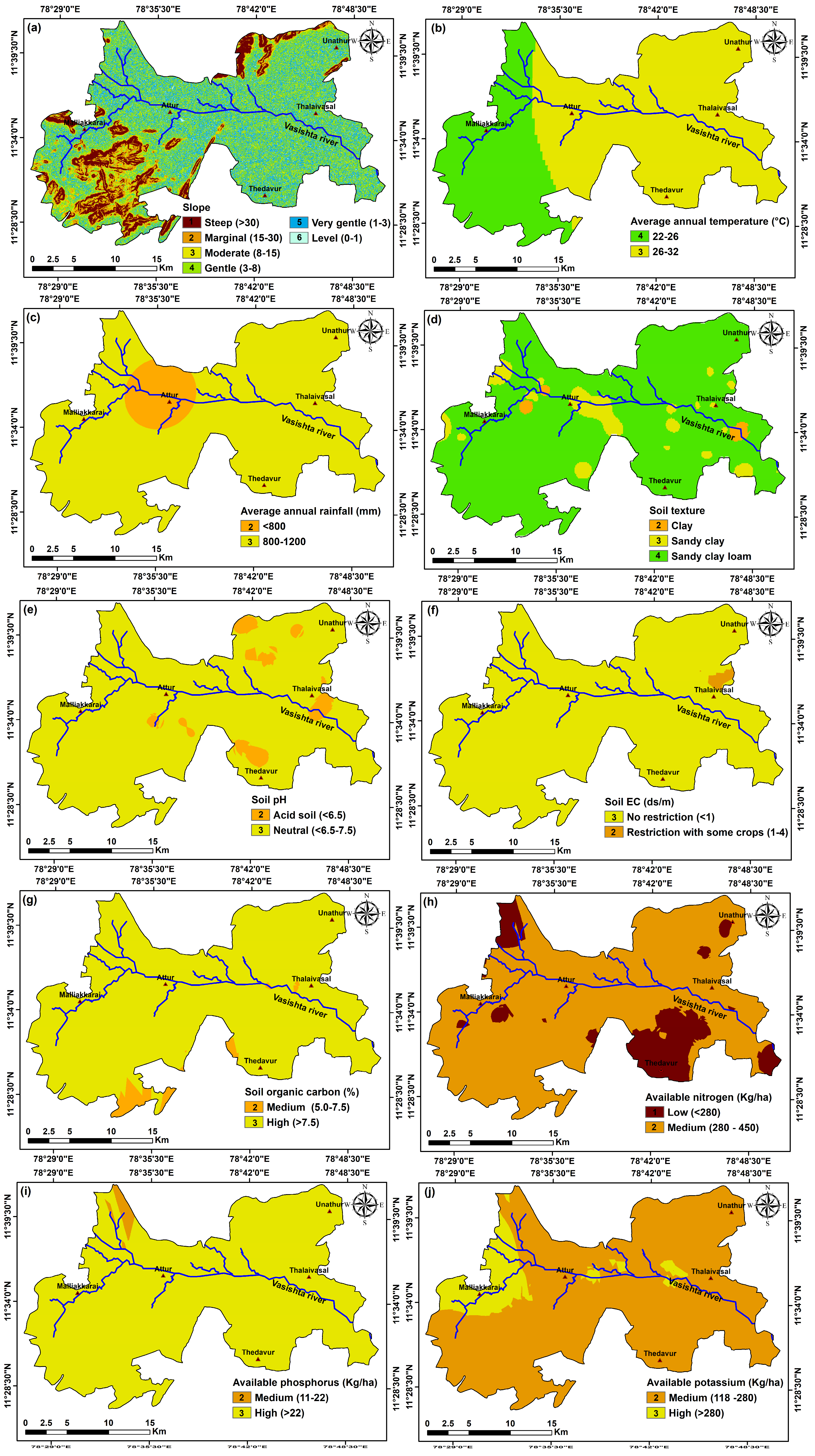
3.2.1. Topographical Factors

Analyzing SRTM-DEM imagery is a commonly utilized method for identifying landform classes with potential agricultural suitability [59]. The height of the Attur region declines progressively from roughly 925 m above sea level (a.s.l.) in its southwestern and northern areas to 126 m (a.s.l.) in the southeastern area (Figure 3a). Generally, Attur features a gentle SL surface (<8%), with certain regions exhibiting a steep SL exceeding 30% (Figure 3b). SL is a known key topographic feature affecting AgLS [6]. A scoring system was devised to evaluate the appropriateness of various SL classes for AgLS (Table 4). This approach allocates ratings according to the SL gradient, with increased values signifying enhanced appropriateness. The classes with a level of 0–1% and a very gentle SL of 1–3% are awarded the highest score of 5, while the gentle SL of 3–8% receives a score of 4 (Table 4 and Figure 7a). A moderate SL (8–15%) is assigned a score of 3, but a strong SL (15–30%) and a steep SL (>30%) are assigned values of 2 and 1, respectively. The gentle SL class encompassed the largest area, measuring around 250.25 km² (Table S1). The groups of level, very gentle, moderate, severe, and very steep SL encompass areas of approximately 40.49, 199.48, 38.31, 38.43, and 58.17 km² of the entire research area, respectively.

3.2.2. Climatic Factors

The spatial distribution map of average maximum and minimum temperatures indicates that elevated values were situated in the northeastern and northwestern regions of the area (Figure 4a,b). The analysis of temperature data indicated that regions with a moderate temperature range (e.g., 22–26 °C) were designated as the most appropriate for agriculture (Figure 7b). Conversely, regions with elevated temperatures (e.g., over 26 °C) were assigned a moderate appropriateness rating. This ranking indicates the possible constraints that excessive heat may put on crop development and productivity [7]. The regional variability map of AAT was produced utilizing the ordinary kriging approach, with class: (22–26 °C) of around 416.57 km² and class: (over 26 °C) spanning around 208.56 km² of the total area of the study region (Figure 7b). The AAR varied between 750 mm and 1092 mm (Figure 4c). Regions characterized by high rainfall are typically deemed more conducive to agriculture, while locations with low rainfall offer the least advantageous conditions [2]. As a result, the region was categorized into two zones: class 1 (<800 mm) and class 2 (800–1200 mm), as seen in Figure 7c. The AAR class 1 and class 2 encompass regions of roughly 55.01 km² and 570.11 km², respectively (Figure 7c and Table S1).

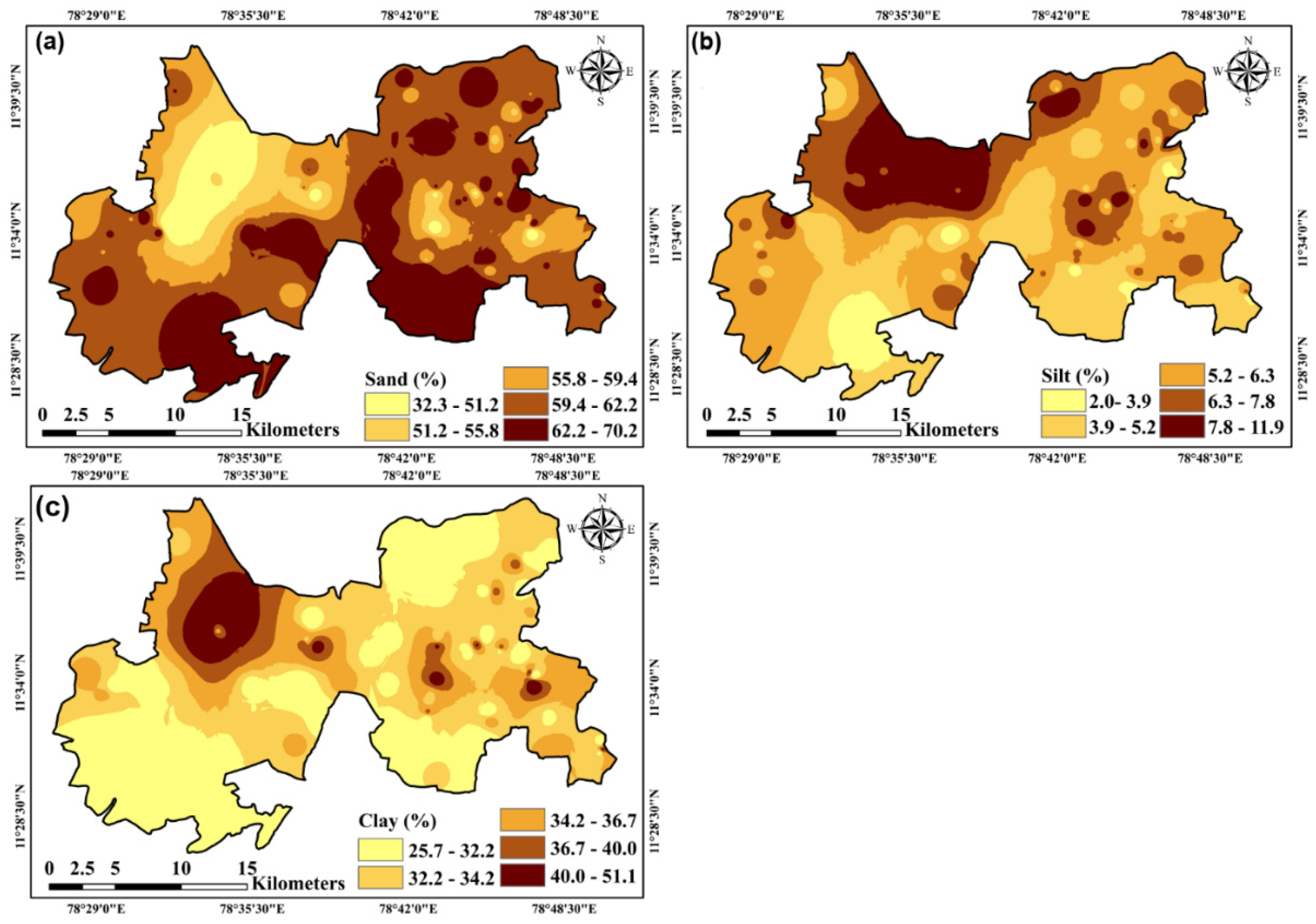
3.2.3. Soil Texture (ST)

ST is essential for determining appropriate agricultural locations [6]. The spatial distribution of near-surface soils in the study area was primarily characterized by sand, clay, and silt contents, averaging 59.72%, 33.86%, and 6.01%, respectively. Sand attained its peak concentration (70.2%) in the southern regions, with a local maximum seen in the northeastern area (Figure 5a). Soils in the northwestern areas were characterized by elevated levels of clay (51.1%) and silt (11.9%) (Figure 5b,c). The ST map illustrated three soil types in Attur Taluk: sandy clay loam, sandy clay, and clay (Figure 7d). Accordingly, Attur soil was deemed appropriate for sandy clay loam, receiving a score of 4, while sandy clay was rated at 2, indicating lesser suitability (Table 4).

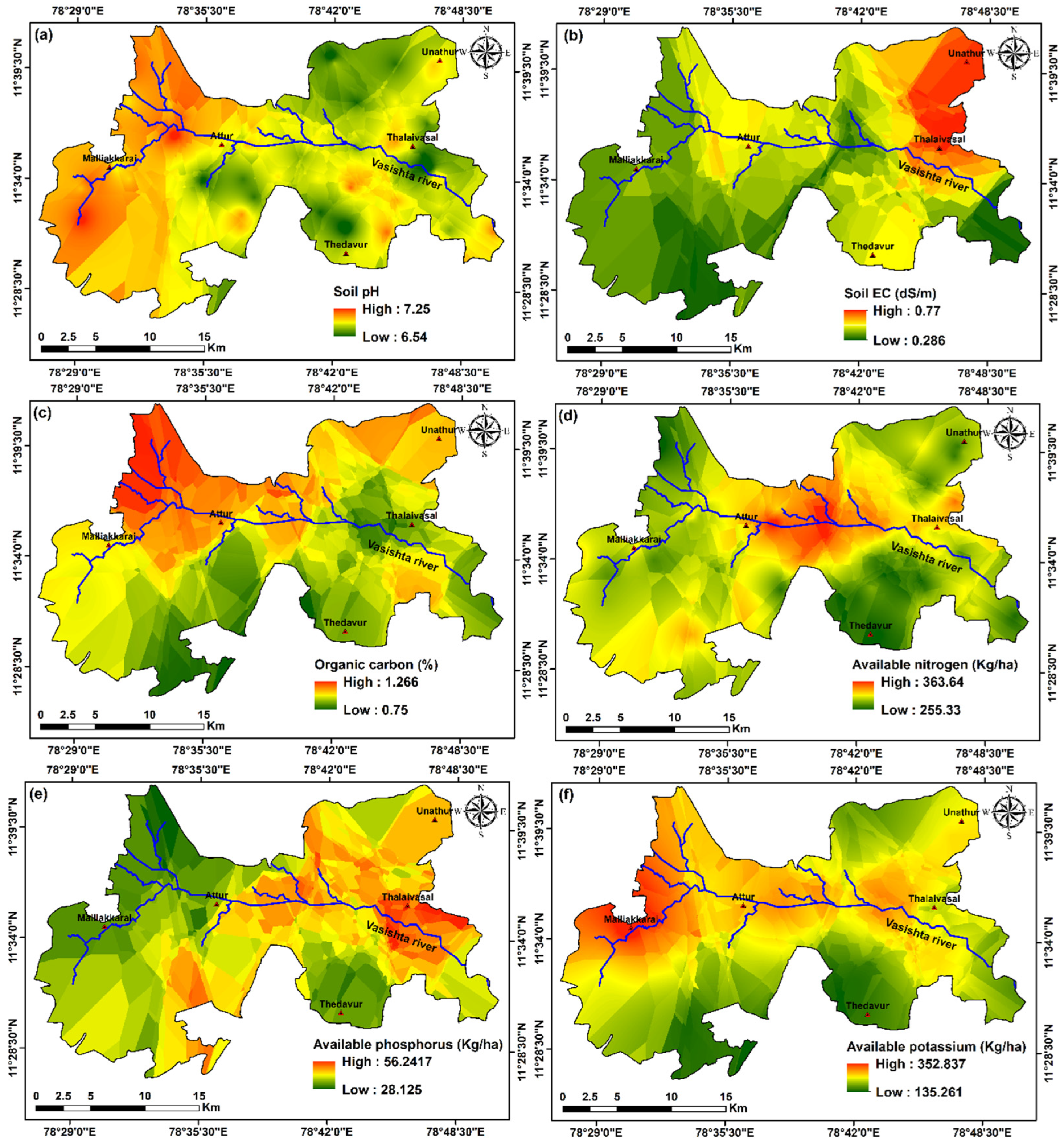
3.2.4. Soil Chemical Contents

The spatial characterization of soil physicochemical parameter distribution is essential for assessing the potential impact of external variables on ecosystems [60]. Figure 6 illustrates the distribution maps of the analyzed soil chemical constituents. The soil pH was elevated in the majority of the research area’s sections (Figure 6a). Two pH categories were identified, acidic (<6.5) and neutral (6.5–7.5), as illustrated in Figure 7e, encompassing areas of 30.00 km² and 595.10 km² (Table S1), respectively. The regional distribution of soil EC indicated that the majority of the Attur region possessed acceptable soil (<1 dS m⁻¹) while exhibiting localized limitations for certain crops (1–4 dS m⁻¹) in the eastern region (Figure 6b and Figure 7f).

Soil nutrients constitute an additional limiting soil characteristic for AgLS, in conjunction with salinity conditions [14]. The current study’s results indicated fluctuations in the concentrations of OC, AN, AP, and AK throughout the study region (Figure 6c–f). The OC map indicated elevated concentrations in the northern parts of the study area (Figure 6c). These regions corresponded with areas designated as extremely favorable for OC concentration exceeding 7.5%, encompassing 609.1 km² of the total area (Table S1). In contrast, the regions (16.00 km²) exhibiting intermediate adaptability were defined by organic carbon levels between 5 and 7.5%. AN varied from 190.40 to 420 kg ha⁻¹, whereas AP had values from 10.40 to 88.30 kg ha⁻¹ (Table 1). The AK concentrations varied from 53.70 to 887.50 kg ha⁻¹. These results align with the data documented by Wani et al. [61]. In addition, favorable suitability mapping is most affected by OC levels over 0.75%, AP levels surpassing 22 kg ha⁻¹, and AK levels more than 280 kg ha⁻¹, as depicted in Figure 7g–i. In addition, medium suitability delineation is most influenced by OC (5–7.5)%, AP (11–22) kg ha⁻¹, AK (11–280) kg ha⁻¹, and AN (280–450) kg ha⁻¹.

3.3. Mapping and Validation of Agricultural Land Suitability (AgLS) Models

This study presents a comprehensive methodology for evaluating land suitability for sustainable agriculture, incorporating thorough evaluations of soil physicochemical parameters, geomorphological characteristics, and climatic variables. Utilizing both statistical and qualitative procedures that were previously discussed, two suitability maps were produced employing different modeling techniques: (1) an equal weighting model yielding an AgLS_Eq map and (2) an FAHP model producing an AgLS_FAHP map. Discrepancies between the two models were evident in the weighting of previously analyzed components (Table 4). Reduced values in the models signified diminished appropriateness, whereas elevated values implied optimal prospective compatibility for agricultural utilization.

The equal weightage approach is the preferred option among many MCDA-WLC approaches for decision support [48], owing to its straightforward implementation in GIS. Considering that each univariate controlling factor exerts only a partial influence on AgLS, AgLS_Eq was created by integrating ten classed maps (Figure 7a–j), each with equal weight (~10%), concerning potential agricultural suitability. AgLS_Eq categorized the research area into various suitability classifications, from permanently unsuitable to highly suitable for agriculture (Figure 8a). The AgLS_Eq map for agricultural applications indicated that 3.16% (19.53 km²) of Attur Taluk was S1, 50.68% (313.71 km²) was S2, 22.04% (136.45 km²) was S3, 17.34% (107.34 km²) was N1, and 6.78% (41.94 km²) was N2 for cultivation (

Table 5. Areas of different agricultural land suitability (AgLS) classes of Attur Taluk, India, using the equal-weighted (AgLS_Eq) and FAHP-weighted (AgLS_FAHP) criteria models.

Suitability Class	AgLSEq			AgLSFAHP
	Area			Area
	(km2)	(ha)	(%)	(km2)	(ha)	(%)
N2	41.94	4194	6.78	48.50	4850	7.82
N1	107.34	10,734	17.34	73.56	7356	11.87
S3	136.45	13,645	22.04	134.47	13,447	21.69
S2	313.71	31,371	50.68	256.16	25,616	41.32
S1	19.53	1953	3.16	107.29	10,729	17.31

Note: S₁ = highly suitable; S₂ = moderately suitable; S₃ = marginally suitable; N₁ = currently unsuitable; N₂ = permanently unsuitable.

).

A crucial element of the FAHP method is acquiring appropriate weights and addressing fuzziness and uncertainty in modeling to enhance the predictive capability of agricultural suitability [17]. The FAHP analysis produced λmax (the largest eigenvalue of the comparative matrix), CI, and CR values of 10.42, 0.042, and 0.032, respectively. These values validated satisfactory consistency throughout all suitability assessment matrices, i.e., CR < 0.1. Table 4 presents the fuzzy geometric mean, fuzzy weight, defuzzification weight, and normalized weight of the primary criterion. The AgLS_FAHP map was produced using normalized weights (Figure 8b). The AgLS_FAHP map for agricultural applications indicated that 17.31% (107.29 km²) of Attur Taluk was S1, 41.32% (256.16 km²) was S2, 21.69% (134.47 km²) was S3, 11.87% (73.56 km²) was N1, and 7.82% (48.50 km²) was N2 for cultivation (Table 5).

Figure 9 gives the AUC of ROC curves for the AgLS maps, generated using both AgLS_Eq and AgLS_FAHP. The AgLS_FAHP map demonstrated reliable performance with an AUC of 0.71, representing a substantial enhancement over the AUC of 0.602 recorded by the AgLS_Eq map. For enhanced validation results, a credible suitability map should indicate that a majority (exceeding 50%) of healthy vegetation is situated in moderately appropriate zones or higher [48]. In the AgLS_Eq map, 58.7% of the current healthy vegetation is located within moderately and highly appropriate areas (Figure 10). The percentage rose markedly to 74.6% for the AgLS_FAHP map. The data indicated that AgLS_FAHP successfully identified regions more conducive to healthy vegetation development and showed higher accuracy than the AgLS_Eq model.

The AgLS_FAHP technique found numerous key parameters influencing land suitability, including AAR, AAT, SL, pH, and EC (Table 4). These factors collectively represented more than 77% of the overall weight, showing their considerable impact on land suitability. Kilic et al. [2] contended that higher SLs can hinder soil formation and restrict the establishment of sufficient root depth for plant growth. Aguilar-Rivera et al. [62] identified the reliance of some crop production suitability on climatic changes through an integrated GIS-FAHP model. This described the demarcation of N2 zones in the southwestern and northern sectors of the AgLS_FAHP map (Figure 8b). Although OC, AN, and ST were essential factors, AP and AK had a relatively minor impact on land suitability for agriculture. Soil nutrients typically demonstrated elevated suitable values throughout the majority of the research area (Figure 7g–j). As a result, optimal places had minimal limitations for existing crops, facilitating intensive agriculture, particularly with irrigation. Moderately appropriate regions, on the other hand, can support agriculture but require careful management to ensure good yields. The results of this investigation corresponded to observations from recent analogous studies in urban riverine settings, as documented by Wu et al. [63]. Moreover, Wu et al. [63] reported the significance of MCDA methodologies by illustrating the efficacy of a fuzzy logic model that incorporates both soil quality and land-use type distribution in their analysis of the Yellow River Delta, China. Furthermore, Sengupta et al. [64] reported the significance of local knowledge by employing FAHP-GIS for AgLS evaluation in the Ranchi area, India. Optimally employing land with significant agricultural potential for sustainable practices is essential to guarantee long-term food security [6]. The current assessment study highlighted the regional variability of soil characteristics, which considerably affected agricultural land viability. In addition, it established a basis for harmonizing agricultural practices, as elaborated in the following section, which examines the connections between the study outcomes and the SDGs.

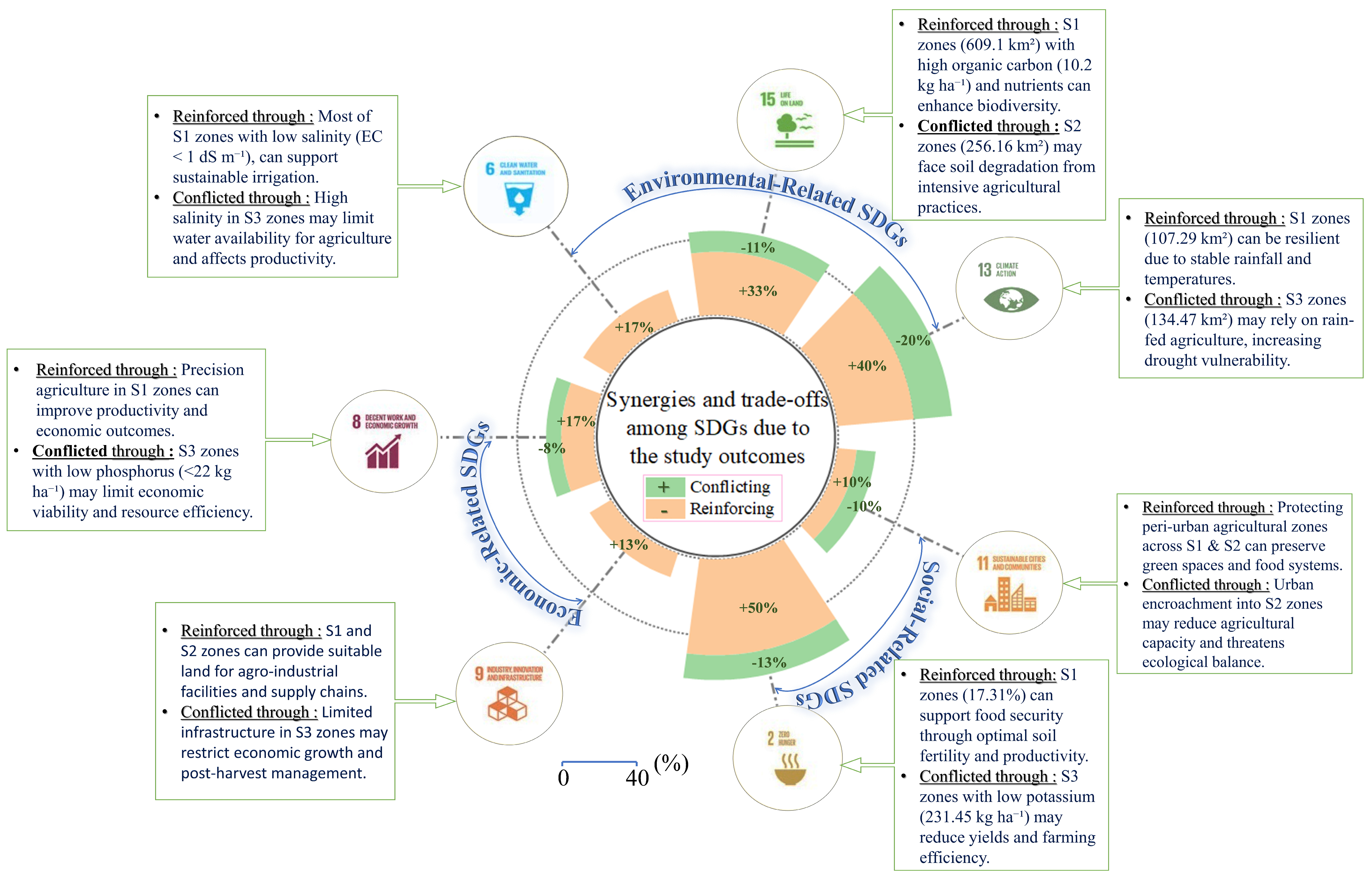
3.4. Correlation of Study Outcomes to Sustainable Development Goals (SDGs)

The hybrid GIS-FAHP–geostatistical approach utilized in this study provided a methodical framework for identifying suitable AgLS in the area of investigation. This methodology enhanced the precision and reliability of land suitability evaluations by incorporating geospatial technology, fuzzy multi-criteria decision analysis, and geostatistical analysis, as reported in previous studies [65]. Additionally, the obtained AgLS in this study can be positively or negatively correlated to SDGs. To illustrate, positive relationships (reinforcing linkages) between AgLS and SDGs enhance sustainable growth by improving resource efficiency and environmental conservation while addressing negative relationships (conflicting linkages) through targeted interventions to mitigate adverse impacts and ensure balanced progress toward sustainability (Figure 11).

3.4.1. Reinforcing Linkages

The hybrid GIS-FAHP–geostatistical approach can reveal significant patterns in advancing SDGs by identifying synergies between effective agricultural land use and sustainability targets. These reinforcing links might highlight the study’s advantages for environmental conservation, economic development, and social growth.

• Environmental-Related SDGs

This study contributes to 40% (two out of five) of SDG 13 targets, specifically addressing Targets 13.1 (resilience to climate-related hazards) and 13.3 (education and capacity building on climate adaptation). S1 zones, covering an area of 107.29 km², exhibit favorable agro-climatic conditions with an AAR of 800–1200 mm and an AAT of 22–26 °C. These conditions can contribute to resilience against climate-related hazards by reducing vulnerability to extreme weather events such as droughts or heat waves. Moderate AAR can ensure sufficient water availability, while AAT within this range can minimize crop stress, supporting stable agricultural productivity. These agro-climatic characteristics can also enable the adoption of drought-resistant crops, which require a moderate but stable water supply. Such crops can reduce reliance on intensive irrigation and enhance climate-resilient agricultural practices. By delineating AgLS zones, the findings can provide a framework to mitigate risks posed by climatic variability and confirm the role of adaptive strategies, such as efficient water use and crop diversification, in promoting climate resilience. These findings align with the role of sustainable agricultural planning, as highlighted by Wang et al. [66].

Additionally, this study can address ~33% (two out of six) of SDG 15 targets, specifically Targets 15.1 (safeguarding ecosystems) and 15.5 (halting biodiversity loss). S1 zones have high levels of organic carbon (10.2 kg ha⁻¹) and essential nutrients such as nitrogen (296.31 kg ha⁻¹), phosphorus (39.68 kg ha⁻¹), and potassium (231.45 kg ha⁻¹). These favorable soil conditions can support ecosystem health by enhancing soil fertility, promoting biodiversity, and aligning agricultural suitability with environmental conservation. In addition, the appropriate management of S1 zones can prevent ecosystem degradation, ensure sustainable soil use, and promote long-term biodiversity. These findings highlight the critical role of maintaining soil health for land conservation and environmental sustainability, as supported by Hussain et al. [59].

Also, this study can contribute to ~17% (one out of six) of SDG 6 targets, specifically Target 6.6 (safeguarding water-related ecosystems). Approximately 33% of S1 zones have EC values below 1 dS m⁻¹, indicating minimal salinity issues and high suitability for sustainable irrigation practices. These low-salinity areas can support efficient water use, reduce the risk of salinity-induced soil degradation, and promote long-term agricultural sustainability. By mapping and prioritizing these zones, this study can provide critical insights for sustainable water management practices. These findings underscore the importance of salinity control in AgLS, as emphasized by Muhaimeed et al. [60].

• Economic-Related SDGs

This study can support ~17% (2 out of 12) of SDG 8 targets, specifically Targets 8.2 (enhancing economic productivity) and 8.3 (supporting entrepreneurship). S1 zones, covering 107.29 km², are highly suitable for implementing precision agriculture, which can improve yields, reduce input costs, and enhance resource efficiency. These practices not only can promote sustainable agricultural production but also create economic opportunities for rural communities by fostering employment and entrepreneurship. These findings demonstrate that optimizing agricultural suitability zones can enhance productivity, increase rural income, and contribute to sustainable economic growth. This aligns with previous studies, such as Ozkan et al. [65], which highlighted the potential of agricultural development to drive rural economic improvement.

In addition, this study can contribute to ~13% (one out of eight) of SDG 9 targets, specifically Target 9.1 (building resilient infrastructure). The spatial mapping of S1 and S2 zones can provide actionable insights for developing agro-industrial facilities in high-potential areas. For instance, establishing post-harvest storage and processing hubs in these zones can minimize crop losses, enhance supply chain efficiency, and promote agricultural resilience. By aligning infrastructure development with land suitability, the study can support the creation of resilient agricultural systems. These systems can boost productivity and sustainability, aligning with the findings of Sengupta et al. [64].

• Social-Related SDGs

This study can contribute to 50% (three out of six) of SDG 2 targets, specifically Targets 2.1 (ending hunger), 2.3 (doubling agricultural productivity), and 2.5 (preserving genetic diversity). S1 zones, which represent 17.31% of the study area, exhibit optimal soil fertility and favorable climatic conditions, making them vital for achieving high agricultural productivity. Prioritizing these zones for intensive and sustainable agriculture can enhance food security, address malnutrition, and support economic stability in rural areas. Additionally, focusing on these high-potential zones can allow for the development of sustainable food systems that preserve biodiversity and genetic resources, aligning with the recommendations of Wang et al. [66].

Moreover, this study can positively connect to 10% (1 out of 10) of the targets of SDG 11, specifically Target 11.3 (sustainable urbanization). The hybrid GIS-FAHP–geostatistical approach can provide actionable insights for equitable urban–rural land utilization by identifying and safeguarding peri-urban agricultural zones. These zones, which often exhibit high agricultural suitability, can be protected to curb urban expansion into areas critical for food production. Integrating AgLS zones into urban planning policies can ensure that peri-urban areas maintain their dual role as green buffers and productive agricultural zones, supporting sustainable urbanization. This aligns with the findings of Hussain et al. [59].

3.4.2. Conflicting Linkages

Although the hybrid GIS-FAHP–geostatistical approach can support numerous targets of SDGs, possible conflicting correlations may exist. These contradictory connections may stem from trade-offs among resource optimization, environmental preservation, and social equality.

• Environmental-Related SDGs

The study can contradict 20% (one out of five) of the targets of SDG 13, specifically Target 13.2 (integrating climate measures into policy). S3 zones, covering 134.47 km², are heavily reliant on rain-fed agriculture, making them particularly vulnerable to droughts and climatic variability. Without implementing adaptive measures such as water conservation, soil management, or drought-resistant cropping systems, these areas can risk low productivity and heightened environmental stress. Addressing the climate vulnerability of marginally suitable zones is essential for achieving long-term resilience, as highlighted by Kilic and Gunal [2].

In addition, this study can negatively match ~11% (one out of nine) of the targets of SDG 15, specifically Target 15.3 (combat desertification). S2 zones, spanning 256.16 km², are at risk of nutrient depletion and soil degradation due to over-intensive agricultural practices. These vulnerabilities can underscore the need for sustainable interventions, such as rotational cropping, organic amendments, and soil conservation techniques, to mitigate desertification risks. The effective management of these zones is critical to preventing long-term productivity loss and ensuring land sustainability, as highlighted by Hussain et al. [59].

• Economic-Related SDGs;

The study can show conflicts with ~8% (1 out of 12) of the targets of SDG 8, specifically Target 8.4 (global resource efficiency). S3 zones, characterized by poor soil fertility and climatic constraints, may lead to inefficient resource use and low economic returns. These findings highlight the importance of reallocating resources to S1 and S2 zones, where higher productivity and better resource efficiency can be achieved. Prioritizing S3 areas for farming may result in increased production costs and reduced profitability, underscoring the need for strategic land-use planning, as supported by Sathiyamurthi et al. [48].

• Social-Related SDGs;

The study can negatively match ~13% (one out of eight) of the targets associated with SDG 2, specifically Target 2.4 (ensuring sustainable food production). S3 zones, with nutrient levels below optimal thresholds (e.g., phosphorus < 22 kg ha⁻¹), can contribute minimally to food production while demanding high resource inputs. These inefficiencies can reduce their potential to support food security and emphasize the need for targeted resource management strategies, such as soil fertility enhancement and precision agriculture techniques, to improve productivity in these zones. This aligns with the findings of Bogunovic et al. [52].

Moreover, this study can negatively meet 10% (1 out of 10) of the targets of SDG 11, specifically Target 11.7 (universal access to green areas). Urban encroachment into S1 and S2 zones, covering 363.45 km², can pose a significant threat to green spaces and peri-urban agricultural buffers. These areas can serve as critical ecological and social assets, and their loss could undermine environmental sustainability and community well-being. The findings highlight the need for stringent zoning regulations and urban planning policies to safeguard these zones and preserve their role as green buffers and food production areas, as emphasized by Sengupta et al. (2020) [64].

Resolving these environmental, economic, and social conflicts is crucial for achieving balanced advancement toward sustainability achievement.

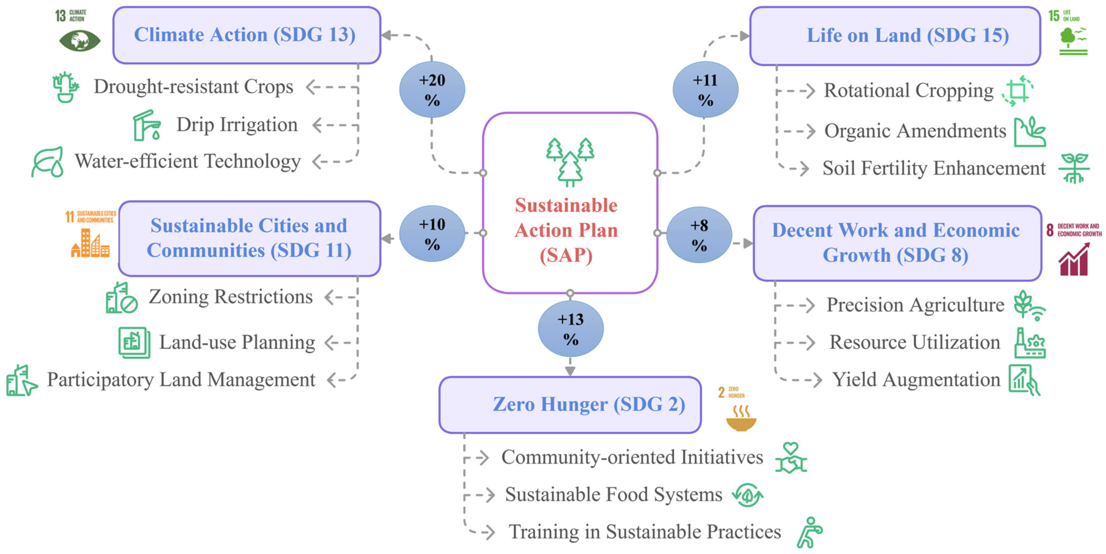
3.4.3. Sustainable Action Plan (SAP)

A thorough SAP is essential to address the conflicts identified in the study, align agricultural practices with long-term sustainability objectives, and avoid negative impacts on SDG targets (Figure 12). For SDG 13 (climate action), reliance on rain-fed agriculture in S3 zones (134.47 km²) may increase vulnerability to drought and climate variability. These challenges highlight the importance of implementing adaptive measures such as drought-resistant crops and advanced irrigation methods, including drip irrigation. Such interventions can reduce reliance on rainfall, enhance water-use efficiency, and stabilize agricultural systems in areas experiencing significant rainfall variability. These adaptive strategies contribute to achieving Target 13.1 (resilience to climate-related hazards), as emphasized by Muhaimeed et al. [60]. By integrating these measures, progress toward SDG 13 can improve by 20% (gaining one additional target out of five).

For SDG 15 (life on land), intensive farming in S2 zones (256.16 km²) may pose a risk of soil degradation due to overutilization. Strategies like rotational cropping and the use of organic amendments, especially in areas where organic carbon levels fall below 8.5 kg ha⁻¹, are essential for restoring soil fertility and ensuring long-term productivity. These interventions can align with Target 15.3 (combat desertification) and support sustainable land management. The nitrogen and potassium levels in these zones, averaging 296.31 kg ha⁻¹ and 231.45 kg ha⁻¹ respectively, can provide a strong basis for targeted soil restoration interventions. Such practices, as highlighted by Chang [18], are crucial for sustaining soil fertility and agricultural productivity. These efforts can improve alignment with SDG 15 by 11% (gaining one additional target out of nine).

For SDG 8 (decent work and economic growth), unsustainable resource use in S3 zones, particularly in areas with phosphorus levels below 22 kg ha⁻¹, may limit their economic potential. Precision agriculture technologies can optimize resource utilization and significantly improve yields in these zones, reducing inefficiencies. Efficient resource allocation and nutrient management can enhance economic contributions from low-potential areas, supporting rural livelihoods and local economies. These measures directly align with Target 8.2 (enhancing economic productivity), as noted by Sathiyamurthi et al. [48]. Implementing these strategies can advance alignment with SDG 8 by 8% (gaining 1 additional target out of 12).

Urban encroachment into S1 and S2 zones, spanning 363.45 km², may pose a significant threat to achieving SDG 11 (sustainable cities and communities) by reducing the agricultural capacity of these areas and diminishing their ecological and economic contributions. Peri-urban zones not only may serve as green buffers but also may function as critical food production hubs, playing an integral role in urban food security and environmental health. This study highlights how protecting these zones through zoning regulations and participatory land-use frameworks can ensure sustainable urban–rural integration. These frameworks should prioritize preserving the agricultural potential of S1 and S2 zones to meet urban demands while maintaining ecological balance. Furthermore, the integration of AgLS findings into urban planning policies can guide sustainable development by aligning infrastructure growth with land suitability, mitigating the risk of losing highly productive agricultural zones. These interventions directly align with Target 11.3 (sustainable urbanization) by promoting equitable and efficient land use, as supported by Hussain et al. [59]. By implementing these measures, alignment with SDG 11 can improve by 10% (gaining 1 additional target out of 10).

Addressing inefficiencies in S3 zones, which contribute minimally to SDG 2 (zero hunger), may require inclusive, community-driven initiatives. Providing training to farmers on sustainable practices and access to essential inputs can increase productivity in these areas. Interventions to improve soil fertility in S3 zones with low potassium (231.45 kg ha⁻¹) and organic carbon can substantially enhance agricultural outputs. These efforts can align with Target 2.3 (doubling agricultural productivity) and Target 2.4 (ensuring sustainable food production), as noted by Bogunovic et al. [52]. These efforts can improve alignment with SDG 2 by 13% (gaining two additional targets out of eight).

The proposed SAP closely aligns with the study’s findings, offering a practical framework for mitigating conflicts and enhancing agricultural systems’ contributions to SDGs. Integrating these measures into policy frameworks ensures that agricultural development can positively impact environmental, economic, and social dimensions, fostering balanced progress toward achieving the SDGs.

4. Limitations and Future Research Directions

This study provides valuable insights into the synergies and trade-offs between AgLS and SDGs. However, several limitations should be acknowledged. The use of generalized agro-climatic thresholds, such as annual average rainfall (AAR: 800–1200 mm) and annual average temperature (AAT: 22–26 °C), may not fully account for localized climate variability or the specific requirements of diverse crops [59]. While these thresholds may provide a broad framework, they may oversimplify complex environmental dynamics, potentially affecting the precision of contributions to SDG 13 (climate action). The reliance on available spatial and environmental data also may limit the inclusion of socio-economic variables, which could have strengthened the analysis in Section 3.4.1 and Section 3.4.3 [63]. Furthermore, while FAHP may minimize bias through expert judgment, it may introduce a degree of subjectivity in assigning weights to decision-making criteria. Lastly, the absence of field-based validation or stakeholder feedback due to time and logistical constraints may limit the real-world applicability of the findings and their direct relevance to broader social and economic systems [17].

Future studies should address these limitations by incorporating fine-scale agro-climatic data and crop-specific thresholds to enhance the accuracy of land suitability analyses [66]. Expanding the scope to include socio-economic variables, such as population density, income levels, and access to markets, can improve correlations with broader SDGs, particularly SDG 8 (decent work and economic growth) and SDG 11 (sustainable cities and communities) [67]. Moreover, conducting field-based validations and engaging stakeholders in participatory planning processes can provide practical insights and strengthen the reliability of results. Refining the FAHP methodology with advanced data-driven approaches, such as machine learning, can further reduce subjectivity and improve decision-making precision [68]. These advancements ensure that future studies can provide a more comprehensive and context-specific understanding of AgLS and its alignment with SDGs, as recommended by Paudel et al. [20], Barletti et al. [69], and Briassoulis et al. [70].

5. Conclusions

This research employed a hybrid GIS-FAHP–geostatistical approach to delineate AgLS in Attur Taluk, India, while examining its implications for synergies and trade-offs with the SDGs. The study illustrated the possibility for enhanced site suitability evaluations by incorporating ten parameters, representing typographical, climatic, and soil characteristics. Geostatistical analysis indicated considerable geographical heterogeneity in soil parameters, especially SL and OC. The AgLS_FAHP map exhibited enhanced accuracy, with AUC = 0.71 for the ROC plot, in comparison with AUC = 0.602 for AgLS_Eq. This high accuracy of the AgLS_FAHP map was confirmed with 74.6% of healthy vegetation zones associated with highly and moderately appropriate areas, in contrast to 58.7% for the AgLS_Eq map. According to the AgLS_FAHP map, suitability mapping designated 17.31% of the area as the S1 zone, 41.32% as the S2 area, and 21.68% as the N2 region. The quantitative investigation of the study outcomes to SDG achievement revealed substantial synergies. The analysis positively addressed 40% of the targets of SDG 13 (climate action) by improving climate resilience through suitability mapping informed by rainfall and temperature variability. For SDG 15 (life on land), 33% of the targets showed positive correlations, especially through the protection of ecosystems and biodiversity via land-use planning that emphasized regions with elevated organic carbon levels. The current research also advanced SDG 2 (zero hunger) by meeting 50% of the targets through the promotion of sustainable food production and the enhancement of productivity in appropriate areas. However, trade-offs were identified, including 20% mismatch with SDG 13 due to reliance on rain-fed agriculture in marginal zones, 11% with SDG 15 due to soil degradation risks, and 13% with SDG 2 resulting from inefficiencies in low-productivity areas. To alleviate these conflicts, an SAP was introduced, encompassing techniques such as drought-resistant crops, enhanced irrigation, and participatory planning. This study can offer a reproducible paradigm for sustainable land-use planning in similar regions worldwide by integrating agricultural development with global sustainability targets. Future studies should incorporate additional socio-economic variables, higher-resolution data, and machine learning techniques to improve MCDA and match more SDGs.

References

1. Saito, Y.; Syvitski, J.P.M. Morphodynamics of deltas under the influence of humans. Glob. Planet. Chang. 2007, 57, 261–282. [Google Scholar]
2. Kilic, O.M.; Gunal, H. Spatial-temporal changes in rainfall erosivity in Turkey using CMIP5 global climate change scenario. Arab. J. Geosci. 2021, 14, 12. [Google Scholar] [CrossRef]
3. IPCC. Climate Change 2013—The Physical Science Basis. In Soil Chemical Analysis; Prentice Hall, Inc.: Englewood Cliffs, NJ, USA, 2013. [Google Scholar]
4. Rama Rao, C.A.; Raju, B.M.K.; Subba Rao, A.V.M.; Rao, K.V.; Rao, V.U.M.; Ramachandran, K.; Venkateswarlu, B.; Sikka, A.K.; Srinivasa Rao, M.; Maheswari, M.; et al. A district level assessment of vulnerability of Indian agriculture to climate change. Curr. Sci. 2016, 110, 1939–1946. [Google Scholar] [CrossRef]
5. Tian, X.; Engel, B.A.; Qian, H.; Hua, E.; Sun, S.; Wang, Y. Will reaching the maximum achievable yield potential meet future global food demand? J. Clean. Prod. 2021, 294, 126285. [Google Scholar] [CrossRef]
6. Saqr, A.M.; Nasr, M.; Fujii, M.; Yoshimura, C.; Ibrahim, M.G. Monitoring of Agricultural Expansion Using Hybrid Classification Method in Southwestern Fringes of Wadi El-Natrun, Egypt: An Appraisal for Sustainable Development. In Environment and Sustainable Development. ACESD 2022. Environmental Science and Engineering; Ujikawa, K., Ishiwatari, M., Hullebusch, E.V., Eds.; Springer: Singapore, 2023; pp. 349–362. [Google Scholar] [CrossRef]
7. Naidu, L.G.K.; Ramamurthy, V.; Challa, O.; Hedge, R.; Krishnan, P. Manual Soil Site Suitability Criteria for Major Crops; NBSS Publication No. 129; National Bureau of Soil Survey and Land Use Planning (NBSS & LUP): Nagpur, Indian, 2006.
8. Alao, J.O.; Ayejoto, D.A.; Fahad, A.; Mohammed, M.A.A.; Saqr, A.M.; Joy, A.O. Environmental Burden of Waste Generation and Management in Nigeria. In Technical Landfills and Waste Management; Springer Water, Part F2824; Springer: Cham, Switzerland, 2024; pp. 27–56. [Google Scholar] [CrossRef]
9. El Baroudy, A.A. Mapping and evaluating land suitability using a GIS-based model. Catena 2006, 140, 96–104. [Google Scholar] [CrossRef]
10. Sharma, R.; Kamble, S.S.; Gunasekaran, A. Big GIS analytics framework for agriculture supply chains: A literature review identifying the current trends and future perspectives. Comput. Electron. Agric. 2018, 155, 103–120. [Google Scholar] [CrossRef]
11. Mendas, A.; Delali, A. Integration of MultiCriteria Decision Analysis in GIS to develop land suitability for agriculture: Application to durum wheat cultivation in the region of Mleta in Algeria. Comput. Electron. Agric. 2012, 83, 117–126. [Google Scholar] [CrossRef]
12. Saqr, A.M.; Nasr, M.; Fujii, M.; Yoshimura, C.; Ibrahim, M.G. Optimal Solution for Increasing Groundwater Pumping by Integrating MODFLOW-USG and Particle Swarm Optimization Algorithm: A Case Study of Wadi El-Natrun, Egypt. In Proceedings of the 2022 12th International Conference on Environment Science and Engineering (ICESE 2022), Environmental Science and Engineering, Beijing, China, 2–5 September 2022; Chen, X., Ed.; Springer: Singapore, 2023; pp. 59–73. [Google Scholar] [CrossRef]
13. Saqr, A.M.; Ibrahim, M.G.; Fujii, M.; Nasr, M. Simulation-Optimization Modeling Techniques for Groundwater Management and Sustainability: A Critical Review. Adv. Eng. Forum 2022, 47, 89–100. [Google Scholar] [CrossRef]
14. Metwally, M.S.; Shaddad, S.M.; Liu, M.; Yao, R.J.; Abdo, A.I.; Li, P.; Jiao, J.; Chen, X. Soil properties spatial variability and delineation of site-specific management zones based on soil fertility using fuzzy clustering in a hilly field in Jianyang, Sichuan, China. Sustainability 2019, 11, 7084. [Google Scholar] [CrossRef]
15. Saha, S.; Sarkar, D.; Mondal, P.; Goswami, S. GIS and multi-criteria decision-making assessment of sites suitability for agriculture in an anabranching site of sooin river, India. Model. Earth Syst. Environ. 2021, 7, 571–588. [Google Scholar] [CrossRef]
16. Saaty, T.L. The Analytic Hierarchy Process: Planning, Priority Setting, Resource Allocation; McGraw-Hill: New York, NY, USA, 1980; pp. 1–287. [Google Scholar]
17. Saqr, A.M.; Ibrahim, M.G.; Fujii, M.; Nasr, M. Sustainable Development Goals (SDGs) Associated with Groundwater Over-Exploitation Vulnerability: Geographic Information System-Based Multi-criteria Decision Analysis. Nat. Resour. Res. 2021, 30, 4255–4276. [Google Scholar] [CrossRef]
18. Chang, D.-Y. Applications of the extent analysis method on fuzzy AHP. Eur. J. Oper. Res. 1996, 95, 649–655. [Google Scholar] [CrossRef]
19. Noman, M.; Ullah, I.; Khan, M.A.; Qazi, A.; Farooq, W.; Saqr, A.; Elsheikh, A. Analysis of overcurrent protective relaying as minimum adopted fault protection for small-scale hydropower plants. Int. J. Environ. Sci. Technol. 2024, 21, 4457–4470. [Google Scholar] [CrossRef]
20. Paudel, G.; Pant, R.R.; Joshi, T.R.; Saqr, A.M.; Ðurin, B.; Cetl, V.; Kamble, P.N.; Bishwakarma, K. Hydrochemical Dynamics and Water Quality Assessment of the Ramsar-Listed Ghodaghodi Lake Complex: Unveiling the Water-Environment Nexus. Water 2024, 16, 3373. [Google Scholar] [CrossRef]
21. Foley, J.A.; Ramankutty, N.; Brauman, K.A.; Cassidy, E.S.; Gerber, J.S.; Johnston, M.; Mueller, N.D.; O’Connell, C.; Ray, D.K.; West, P.C.; et al. Solutions for a cultivated planet. Nature 2011, 478, 337–342. [Google Scholar] [CrossRef] [PubMed]
22. Choudhary, K.; Boori, M.S.; Shi, W.; Valiev, A.; Kupriyanov, A. Agricultural land suitability assessment for sustainable development using remote sensing techniques with analytic hierarchy process. Remote Sens. Appl. Soc. Environ. 2023, 32, 101051. [Google Scholar] [CrossRef]
23. Panneerselvam, B.; Muniraj, K.; Thomas, M.; Ravichandran, N.; Bidorn, B. Identifying influencing groundwater parameter on human health associate with irrigation indices using the Automatic Linear Model (ALM) in a semi-arid region in India. Environ. Res. 2021, 202, 111778. [Google Scholar] [CrossRef] [PubMed]
24. Pathak, H.; Fagodiya, R.K. Nutrient Budget in Indian Agriculture During 1970–2018: Assessing Inputs and Outputs of Nitrogen, Phosphorus, and Potassium. J. Soil Sci. Plant Nutr. 2022, 22, 1832–1845. [Google Scholar] [CrossRef]
25. Sundaralingam, K.; Biswal, T.K.; Thirukumaran, V. Strain analysis of the Salem-Attur shear zone of Southern Granulite Terrane around Salem, Tamil Nadu. J. Geol. Soc. India 2017, 89, 5–11. [Google Scholar] [CrossRef]
26. Şener, Ş.; Şener, E.; Nas, B.; Karagüzel, R. Combining AHP with GIS for landfill site selection: A case study in the Lake Beyşehir catchment area (Konya, Turkey). Waste Manag. 2010, 30, 2037–2046. [Google Scholar] [CrossRef] [PubMed]
27. Roy, S.; Singha, N.; Bose, A.; Basak, D.; Chowdhury, I.R. Multi-influencing factor (MIF) and RS–GIS-based determination of agriculture site suitability for achieving sustainable development of Sub-Himalayan region, India. Environ. Dev. Sustain. 2023, 25, 7101–7133. [Google Scholar] [CrossRef]
28. Moshago, S.; Regassa, A.; Yitbarek, T. Characterization and Classification of Soils and Land Suitability Evaluation for the Production of Major Crops at Anzecha Watershed, Gurage Zone, Ethiopia. Appl. Environ. Soil Sci. 2022, 2022, 9733102. [Google Scholar] [CrossRef]
29. USGS. Homepage. Available online: https://earthexplorer.usgs.gov/ (accessed on 3 December 2024).
30. Available online: https://globalweather.tamu.edu/ (accessed on 3 December 2024).
31. Ghimire, U.; Akhtar, T.; Shrestha, N.K.; Paul, P.K.; Schürz, C.; Srinivasan, R.; Daggupati, P. A Long-term Global Comparison of IMERG and CFSR with Surface Precipitation Stations. Water Resour. Manag. 2022, 36, 5695–5709. [Google Scholar] [CrossRef]
32. Available online: https://tnau.ac.in/site/kvk-salem/soil-and-water-testing-3/ (accessed on 23 June 2023).
33. Jackson, M.L. Soil chemical analysis. J. Frankl. Inst. 1958, 265, 356. [Google Scholar] [CrossRef]
34. Bouyoucos, G.J. The hydrometer as a new method for the mechanical analysis of soils. Soil Sci. 1927, 23, 343–353. [Google Scholar] [CrossRef]
35. Black, I.; Walkley, A.J. Estimation of soil organic carbon by the chromic acid titration method. Soil Sci. 1934, 37, 29–38. [Google Scholar]
36. Subbiah, B.V.; Asija, G.L. A rapid procedure for determination of available nitrogen in soils. Curr. Sci. 1956, 25, 259–260. [Google Scholar]
37. Olsen, S.R.; Cole, C.V.; Watandbe, F.; Dean, L. Estimation of Available Phosphorus in Soil by Extraction with sodium Bicarbonate. J. Chem. Inf. Model. 1954, 53, 1689–1699. [Google Scholar]
38. Stanford, S.; English, L. Use of flame photometer in rapid soil tests of K and Ca. J. Agron. 1949, 41, 446–447. [Google Scholar] [CrossRef]
39. Shit, P.K.; Bhunia, G.S.; Maiti, R. Spatial analysis of soil properties using GIS based geostatistics models. Model. Earth Syst. Environ. 2016, 2, 2. [Google Scholar] [CrossRef]
40. Selmy, S.; El-Aziz, S.A.; El-Desoky, A.; El-Sayed, M. Characterizing, predicting, and mapping of soil spatial variability in Gharb El-Mawhoub area of Dakhla Oasis using geostatistics and GIS approaches. J. Saudi Soc. Agric. Sci. 2022, 21, 383–396. [Google Scholar] [CrossRef]
41. Burrough, P.A.; McDonnell, R.A. Principles of Geographical Information Systems; Taylor & Francis, Ltd.: Abingdon, UK, 1998; Volume 75, p. 422. [Google Scholar]
42. Siska, P.P.; Goovaerts, P.; Hung, I.K.; Bryant, V.M. Predicting ordinary kriging errors caused by surface roughness and dissectivity. Earth Surf. Process. Landf. 2005, 30, 601–612. [Google Scholar] [CrossRef]
43. Mikhailov, L.; Tsvetinov, P. Evaluation of services using a fuzzy analytic hierarchy process. Appl. Soft Comput. J. 2004, 5, 23–33. [Google Scholar] [CrossRef]
44. Reddy, G.M. Trapezoidal fuzzy numbers in extent analysis method in fuzzy AHP. Int. J. Concept. Comput. Inf. Technol. 2015, 3, 69–71. [Google Scholar]
45. Buckley, J.J.; Feuring, T.; Hayashi, Y. Fuzzy hierarchical analysis. In Proceedings of the 1999 IEEE International Fuzzy Systems. Conference Proceedings (Cat. No.99CH36315), Seoul, Republic of Korea, 22–25 August 1999; Volume 2. [Google Scholar]
46. Meyer, V.; Scheuer, S.; Haase, D. A multicriteria approach for flood risk mapping exemplified at the Mulde river, Germany. Nat. Hazards 2009, 48, 17–39. [Google Scholar] [CrossRef]
47. Aly, M.H.; Giardino, J.R.; Klein, A.G. Suitability assessment for New Minia City, Egypt: A GIS approach to engineering geology. Environ. Eng. Geosci. 2005, 11, 259–269. [Google Scholar] [CrossRef]
48. Sathiyamurthi, S.; Subbarayan, S.; Ramya, M.; Sivasakthi, M.; Gobi, R.; Qaysi, S.; Praveen Kumar, S.; Lee, J.; Alarifi, N.; Wahba, M.; et al. Advancing Agricultural Land Suitability in Urbanized Semi-Arid Environments: Insights from Geospatial and Machine Learning Approaches. ISPRS Int. J. Geo-Inf. 2024, 13, 436. [Google Scholar] [CrossRef]
49. FAO. A Framework for Land Evaluation; Soils Bulletin No. 32; FAO: Rome, Italy, 1976; pp. 59–92. Available online: https://www.fao.org/3/x5310e/x5310e00.htm (accessed on 3 December 2024).
50. Sepehri, M.; Malekinezhad, H.; Jahanbakhshi, F.; Ildoromi, A.R.; Chezgi, J.; Ghorbanzadeh, O.; Naghipour, E. Integration of interval rough AHP and fuzzy logic for assessment of flood prone areas at the regional scale. Acta Geophys. 2020, 68, 477–493. [Google Scholar] [CrossRef]
51. Das, S. Geospatial mapping of flood susceptibility and hydro-geomorphic response to the floods in Ulhas basin, India. Remote Sens. Appl. Soc. Environ. 2019, 14, 60–74. [Google Scholar] [CrossRef]
52. Bogunovic, I.; Mesic, M.; Zgorelec, Z.; Jurisic, A.; Bilandzija, D. Spatial variation of soil nutrients on sandy-loam soil. Soil Tillage Res. 2014, 144, 174–183. [Google Scholar] [CrossRef]
53. Wilding, L.P. Spatial variability: Its documentation, accommodation and implication to soil surveys. In Soil Spatial Variability; Pudoc: Wageningen, The Netherlands, 1985; pp. 166–189. [Google Scholar]
54. Trigalet, S.; Gabarrón-Galeote, M.A.; Van Oost, K.; van Wesemael, B. Changes in soil organic carbon pools along a chronosequence of land abandonment in southern Spain. Geoderma 2016, 268, 14–21. [Google Scholar] [CrossRef]
55. Cooksey, R.W. Descriptive Statistics for Summarising Data. In Illustrating Statistical Procedures: Finding Meaning in Quantitative Data; Springer: Singapore, 2020; pp. 61–139. [Google Scholar] [CrossRef]
56. Soropa, G.; Mbisva, O.M.; Nyamangara, J.; Nyakatawa, E.Z.; Nyapwere, N.; Lark, R.M. Spatial variability and mapping of soil fertility status in a high-potential smallholder farming area under sub-humid conditions in Zimbabwe. SN Appl. Sci. 2021, 3, 4. [Google Scholar] [CrossRef]
57. Mousavi, S.J.; Parnianpour, M.; Askary-Ashtiani, A.R.; Hadian, M.R.; Rostamian, A.; Montazeri, A. Translation and validation study of the Persian version of the Arthritis Impact Measurement Scales 2 (AIMS2) in patients with osteoarthritis of the knee. BMC Musculoskelet. Disord. 2009, 10, 95. [Google Scholar] [CrossRef]
58. Behera, S.K.; Mathur, R.K.; Shukla, A.K.; Suresh, K.; Prakash, C. Spatial variability of soil properties and delineation of soil management zones of oil palm plantations grown in a hot and humid tropical region of southern India. Catena 2018, 165, 251–259. [Google Scholar] [CrossRef]
59. Hussain, S.; Nasim, W.; Mubeen, M.; Fahad, S.; Tariq, A.; Karuppannan, S.; Alqadhi, S.; Mallick, J.; Almohamad, H.; Ghassan Abdo, H. Agricultural land suitability analysis of Southern Punjab, Pakistan using analytical hierarchy process (AHP) and multi-criteria decision analysis (MCDA) techniques. Cogent Food Agric. 2024, 10, 2294540. [Google Scholar] [CrossRef]
60. Muhaimeed, A.S.; al-Jeboory, S.R.; Saliem, K.A.; Burt, R.; Chiaretti, J.V. Genesis and Classification of Selected Soils in an Arid Region of Central Iraq. Soil Horiz. 2013, 54, 1–13. [Google Scholar] [CrossRef]
61. Wani, M.A.; Shaista, N.; Wani, Z.M. Spatial Variability of Some Chemical and Physical Soil Properties in Bandipora District of Lesser Himalayas. J. Indian Soc. Remote Sens. 2017, 45, 611–620. [Google Scholar] [CrossRef]
62. Aguilar-Rivera, N.; Algara-Siller, M.; Olvera-Vargas, L.A.; Michel-Cuello, C. Land management in Mexican sugarcane crop fields. Land Use Policy 2018, 78, 763–780. [Google Scholar] [CrossRef]
63. Wu, C.; Liu, G.; Huang, C.; Liu, Q. Soil quality assessment in Yellow River Delta: Establishing a minimum data set and fuzzy logic model. Geoderma 2019, 334, 82–89. [Google Scholar] [CrossRef]
64. Sengupta, S.; Mohinuddin, S.; Arif, M.; Sengupta, B.; Zhang, W. Assessment of agricultural land suitability using GIS and fuzzy analytical hierarchy process approach in Ranchi District, India. Geocarto Int. 2022, 37, 13337–13368. [Google Scholar] [CrossRef]
65. Özkan, B.; Dengiz, O.; Turan, İ.D. Site suitability analysis for potential agricultural land with spatial fuzzy multi-criteria decision analysis in regional scale under semi-arid terrestrial ecosystem. Sci. Rep. 2020, 10, 22074. [Google Scholar] [CrossRef] [PubMed]
66. Wang, X.; Lian, Q.; Qu, P.; Yang, Q. TBCA: Prediction of Transcription Factor Binding Sites Using a Deep Neural Network With Lightweight Attention Mechanism. IEEE J. Biomed. Health Inform. 2024, 28, 2397–2407. [Google Scholar] [CrossRef] [PubMed]
67. Dessie, G. Forest Decline in South Central Ethiopia Extent, History and Process. Doctoral Dissertation, Stockholm University, Stockholm, Sweden, 2007; p. 90. [Google Scholar]
68. Anand, A.; Deb, C. The potential of remote sensing and GIS in urban building energy modelling. Energy Built Environ. 2024, 5, 957–969. [Google Scholar] [CrossRef]
69. Sarmiento Barletti, J.P.; Larson, A.M.; Hewlett, C.; Delgado, D. Designing for engagement: A Realist Synthesis Review of how context affects the outcomes of multi-stakeholder forums on land use and/or land-use change. World Dev. 2020, 127, 104753. [Google Scholar] [CrossRef]
70. Briassoulis, H. Combating land degradation and desertification: The land-use planning quandary. Land 2019, 8, 27. [Google Scholar] [CrossRef]
Figure 1. (a) Geographic location of the study area in South Asia; (b) Administrative map of Tamil Nadu District in southern India; (c) Detailed map of Attur Taluk, indicating soil sampling sites and the current distribution of healthy vegetation lands used as inventory data.
Sustainability 17 00809 g001
Figure 2. Methodology flowchart of the research study in Attur Taluk, India.
Sustainability 17 00809 g002
Figure 3. Spatial variability map of topographical factors of Attur Taluk, India: (a) elevation and (b) slope (SL).
Sustainability 17 00809 g003
Figure 4. Spatial variability map of climatic factors: (a) minimum annual temperature, (b) maximum annual temperature, and (c) average annual rainfall (AAR).
Sustainability 17 00809 g004
Figure 5. Spatial variability map of soil physical characteristics in the study area: (a) sand (%), (b) silt (%), and (c) clay (%).
Sustainability 17 00809 g005
Figure 6. Spatial variability map of soil chemical factors of Attur Taluk, India: (a) potential of hydrogen (pH), (b) electrical conductivity (EC), (c) organic carbon (OC), (d) available nitrogen (AN), (e) available phosphorus (AP), and (f) available potassium (AK).
Sustainability 17 00809 g006
Figure 7. Ten thematic rated factors of agricultural land suitability (AgLS) of Attur Taluk, India: (a) slope (SL), (b) average annual temperature (AAT), (c) average annual rainfall (AAR), (d) soil texture (ST), (e) potential of hydrogen (pH), (f) electrical conductivity (EC), (g) available organic carbon (OC), (h) available nitrogen (AN), (i) available phosphorus (AP), and (j) available potassium (AK).
Sustainability 17 00809 g007
Figure 8. Final agriculture land suitability (AgLS) maps of Attur Taluk, India: (a) the equal-weighted (AgLSEq) map and (b) the fuzzy analytical hierarchy process (FAHP)-weighted (AgLSFAHP) map.
Sustainability 17 00809 g008
Figure 9. Area under the curve (AUC) of receiver operating characteristic (ROC) plot for the validation of the agricultural land suitability (AgLS) maps of Attur Taluk, India, using different models.
Sustainability 17 00809 g009
Figure 10. Validation of agricultural land suitability (AgLS) maps of Attur Taluk, India, using different approaches.
Sustainability 17 00809 g010
Figure 11. Quantitative correlation of synergies/trade-offs between the study outcomes of land suitability in Attur Taluk, India, and sustainable development goals (SDGs).
Sustainability 17 00809 g011
Figure 12. Sustainable action plan (SAP) along with enhancement percentages to mitigate conflicting linkages to sustainable development goals (SDGs) in Attur Taluk, India.
Sustainability 17 00809 g012