Optimizing Modular Vehicle Public Transportation Services with Short-Turning Strategy and Decoupling/Coupling Operations

Abstract

In public transportation systems, the passenger demand during peak hours is characterized by over-saturation at intermediate stops and directional imbalances, and the traditional single scheduling strategy and fixed capacity cannot solve the contradiction between the demand and capacity mismatch. In order to accurately match demand and capacity, this paper proposes a method to optimize the service of a public transportation system by using a short-turning strategy combined with decoupled/coupled operation of modular vehicles (MVs). The short-turning strategy is used to alleviate the heavy passenger flow at intermediate stations, and the decoupling/coupling operations of MVs are employed to flexibly adjust the capacity levels in different directions. Considering urban space limitations, depots for storing modular units (MUs) are only set up at the starting and ending stations of bidirectional lines. MVs can not only adjust the departure capacity at the starting station but also consider whether to decouple/couple at turnaround stations for short-turning trips to achieve a more effective supply–demand match, with the decoupled/coupled MUs being deadheaded from or provided by the depot. We formulated this problem as an integer nonlinear programming (INLP) model, jointly optimizing the departure intervals of each trip, the capacity of MVs, the turnaround scheme for short-turning trips, and the decoupling/coupling scheme for MVs at turnaround stations, with the aim of minimizing passenger waiting time costs and vehicle operating costs. To facilitate a solution, we equivalently transformed some nonlinear terms in the model, which was then solved by the commercial solver Gurobi. The numerical study shows that, compared with the traditional full-length strategy combined with conventional buses, the model proposed in this paper can reduce the total system cost by about 19.59%. In particular, it can achieve precise matching between passenger demand and transport capacity, thereby reducing the passenger waiting time cost by about 29.99%. Compared with the full-length strategy combined with MVs, the total system cost is also reduced by about 14.65%. The research results contribute to enhancing the service quality and efficiency of public transportation systems, which is of great significance to the sustainable development of these systems.

1. Introduction

Transportation is one of the main sources of carbon emissions; to effectively reduce transportation-related carbon emissions, it is necessary to significantly enhance the attractiveness of public transportation and optimize its service capabilities [1]. Public transportation is a vital mode of travel for urban residents and plays a significant role in alleviating traffic congestion and achieving sustainable development [2,3]. However, with the acceleration of urbanization, the demand for passenger traffic continues to grow, and the contradiction between the supply and demand of urban public transportation systems becomes increasingly prominent [4]. Due to the different functional orientations of various urban areas, there are differences in passenger demand for the up and down directions of bus routes and at each station along the route during peak hours. Traditional public transportation scheduling patterns are singular, with fixed vehicle capacity and fixed departure times, which can meet off-peak demands but cannot effectively adapt to the varying passenger demands during peak hours. This leads to excessively long passenger wait times and high vehicle operation costs, severely reducing the service quality and operational efficiency of the public transportation system [5]. Therefore, effective operational schemes are needed to improve the matching of supply and demand within urban public transportation systems.

In recent years, to alleviate the phenomenon of passenger saturation at peak times in some stations and partial sections, the most commonly used control strategies in public transportation systems include short-turning [6], skip-stop [7], and express [8], etc. These strategies allow buses to skip some stops, thereby reducing the total waiting time for passengers. The focus of this paper’s research is the short-turning strategy, which, based on the traditional single-route bus, opens short-turning vehicles. In response to the phenomenon of high demand passenger flow between some stations and low demand passenger flow between other stations on the bus line, short-turning vehicles can alleviate the local large passenger flow by circulating within a certain sub-section [9,10,11].

In addition, an emerging technology of modular vehicles (MVs) provides a new direction for the development of urban buses [12,13]. This technology uses modular units (MUs) of the same length and capacity, and dynamically adjusts the vehicle capacity through physical decoupling/coupling between the MUs, which can adapt to uneven passenger demand [14]. Currently, the technology has been field-tested in a number of locations, such as Dubai, where MVs developed by NEXT Future Transportation Inc. (Delaware, OH, USA) have been tested.

In view of these benefits, and in order to better balance the contradiction between demand and capacity, this paper adopts a short-turning strategy in combination with MVs technology to optimize the service of the public transportation system, and takes into account the reality that it is not possible to arrange MU-containing depots at all stops in practice, and only sets up two depots for storing the MUs at the starting stops of the bi-directional routes. Work in the literature on short-turning strategies has typically focused on optimizing service schemes for a single type of vehicle, without taking into account the directional imbalance in passenger demand. In contrast, in this study, in addition to the ability of MVs to perform decoupling/coupling operations to flexibly adjust the first-stop departure capacity at the starting station of a bidirectional route, it is considered whether or not decoupling/coupling operations are necessary for the decision-making of the turnaround station of a short-turning vehicle in order to obtain a more effective matching of supply and demand. Specifically, an integer nonlinear programming (INLP) model was developed in this study to determine the departure interval of each trip of the bus system at the first stop and the capacity of MV, the turnaround scheme for short-turning trips, and the decoupling/coupling scheme for MVs at the turnaround stops, which can minimize the cost of waiting time for passengers and the cost of vehicle operation. The main contributions of this paper are summarized as follows:

(1)

Aiming at the problem of saturated passenger flow at local interval stops and unbalanced passenger flow in the up and down directions of a bidirectional bus route during peak hours, this paper jointly optimizes the departure interval of each trip and the capacity of MV, the turnaround scheme of short-turning vehicles, and the decoupling/coupling scheme of MVs at turnaround stops to improve the matching degree between the bus system’s capacity and passenger demand.

(2)

We propose an integer nonlinear programming (INLP) model to simulate the service of MVs with short-turning strategies in public transportation systems, with the objective of minimizing the total sum of passenger waiting time costs and vehicle operating costs. To directly solve the model using the commercial solver Gurobi version 12.0.0, some nonlinear and non-quadratic terms in the model are equivalently replaced.

(3)

The proposed model is tested through numerical studies. The model is compared with two benchmark operation strategies to demonstrate the advantage of MV technology combined with short-turning strategies in reducing the total system cost.

The rest of the paper is organized as follows. In Section 2, we review the literature on short-turning strategies and MVs. In Section 3, we introduce the problem description and notation. In Section 4, we present an integer nonlinear programming (INLP) model to describe the problem, which is solved using the commercial solver Gurobi version 12.0.0 after the equivalent transformation process. In Section 5, we validate the proposed model through a numerical study. In Section 6, we draw some conclusions and future research directions.

2. Literature Review

This section reviews the literature on short-turning strategies and modular vehicles, respectively.

2.1. Short-Turning Strategies

Passenger demand at stations during peak hours is unevenly distributed; in order to improve the operational efficiency and service quality of the bus system, many scholars have proposed different operational strategies, such as short-turning, skip-stop and express. In recent years, the short-turning strategy has been widely applied in bus systems [10]. Zhang et al. [15] conducted research on high-demand bus networks and proposed an integrated strategy combining stationing and short-turning to meet the unbalanced and asymmetric demands of bus routes, aiming to minimize costs to optimize departure frequencies. Wang et al. [16] proposed a real-time short-turning strategy based on passenger choice behavior to improve the service level of bus stations with high passenger demand during peak hours. By optimizing the short-turning trip plan and the starting and ending stations of short-turning, the strategy aims to minimize passenger waiting time. Gkiotsalitis et al. [17] proposed a method for generating candidate short-turning and sub-line routes based on rules. By flexibly assigning bus routes to match changing passenger demands, this method can significantly reduce passenger waiting time and operating costs. Bie et al. [18] proposed a combined operation mode of full-route and short-turning strategies to solve the problem of uneven passenger distribution at different stations. By using the short-turning strategy to relieve passenger flow at some stations, the transportation capacity of buses can be matched with passenger demand, effectively reducing operating costs. Zhang et al. [19] introduced the short-turning strategy in battery electric bus systems to deal with uneven passenger demand during peak hours. By deciding the frequency of short-turning routes and the charging schedule, the strategy aims to minimize passenger waiting time costs and system operating costs. Subsequently, Zhang et al. [20] integrated short-turning and interlining strategies to address the issue of insufficient bus utilization during peak hours. They jointly optimized the planning of short-turning and interlining routes, departure frequencies, and battery capacity to improve vehicle utilization and reduce operating costs. Yanık et al. [21] considering the limited capacity of buses, designed a bus route with a short-turning service mode to maximize the reduction of overcapacity and shortage as well as passenger time-related costs, effectively improving the problem of insufficient transportation capacity.

The above studies have shown that the short-turning strategy is advantageous in dealing with the problem of uneven passenger demand on bus routes during peak hours. The short-turning strategy serves more passengers by increasing the frequency of vehicle service between high-demand stop intervals, and is able to reduce passenger waiting time as well as vehicle fullness. However, most existing studies only consider fixed-capacity vehicles in combination with the short-turning strategy, which is unable to provide a matching level of supply for the directionally unbalanced passenger demand during peak hours. Therefore, this study introduces the MV technology based on the short-turning strategy, which adjusts the capacity size by decoupling/coupling operation at the turnaround station of the short-turning trips, in addition to flexibly changing the capacity of the MV at the first station.

2.2. Modular Vehicles

MVs, as an emerging mode of transportation, have attracted extensive attention from scholars as they are able to achieve autonomous decoupling and coupling on urban roads using automation technology, providing greater flexibility in adjusting the capacity of individual vehicles. Most of the existing related literature focuses on the joint optimization of fixed bus route schedules and vehicle formation plans by considering MVs that can be decoupled/coupled at terminals or designated stops. For example, Chen et al. [22] proposed a discrete modeling approach to jointly optimize the scheduling intervals and capacities of MVs by considering the cost of passenger waiting time and energy consumption, and the MVs can be decoupled/coupled to obtain different capacities. Subsequently, Chen et al. [23] proposed a continuous approximation (CA) model that can effectively provide optimal solutions for the design of bus operation based on MVs technology, which are difficult to find the exact optimal solutions using discrete modeling methods. Dai et al. [24] considered the joint design problem of bus dispatch headway and modular automated vehicle capacity for a bus system with a mixture of manually driven vehicles and modular automated vehicles, with the goal of minimizing bus operating costs and passenger costs. Zhang et al. [25] proposed a new modular automated vehicle service model at the bus stop level, which combines the technique of decoupling/coupling MVs on the move and the skip-stop strategy to decide the number of MVs required per trip, the departure interval, the decoupling/coupling scheme of the MVs and the skip-stop scheme, and is capable of minimizing the total cost of bus operations and passengers as well as save energy consumption. Dakic et al. [26] proposed a novel flexible bus scheduling system that effectively reduces the total system cost by adjusting the optimal composition of MUs and the optimal service frequency of the dispatched vehicles on each bus route through changes in passenger demand.

All of the above studies provide for a MU depot to be set up at the start and end stations of the line, thus storing/providing MUs for decoupling/coupling operations of the MVs. There are also studies that assume a MU depot at the intermediate stops of the line, for example, Liu et al. [27] proposed a joint optimization model for bus schedules and bus formation planning that allows all available MUs in the intermediate depot to be able to join the modular bus in either direction, and the results show that a public transportation system based on modular automated vehicles can better trade-off the vehicle operating costs and passenger waiting time costs. Tian et al. [28] proposed a mixed integer nonlinear programming (MINLP) model to determine the optimal scheduling and MU formation on a single bus route with time-dependent travel demand by considering the limited availability of MUs at the stops and their cost of decoupling/coupling. The case study demonstrated that MV bus services offer significant advantages in reducing operating and passenger costs. Xia et al. [29] optimized the MVs schedules and dynamic capacity allocation plans by allowing MVs to change their capacity at any stop in their study, taking into account time-dependent travel times and uncertain passenger demand. The case study shows that the proposed method is effective in reducing passenger and operator costs.

The above studies show that MVs can dynamically adjust their capacity through decoupling/coupling operations, which can effectively meet the demand of unevenly distributed passenger flow at peak hours. Most of the studies assume that depots for storing MUs are set up at the intermediate stations of the line, but the reality is that it is not possible to set up storage depots at each station of the line due to the space limitation in the city. Therefore, this paper only sets up storage depots at the starting and ending stations of the bus route, and the MUs for short-turning operations are provided/stored by depots through deadheading.

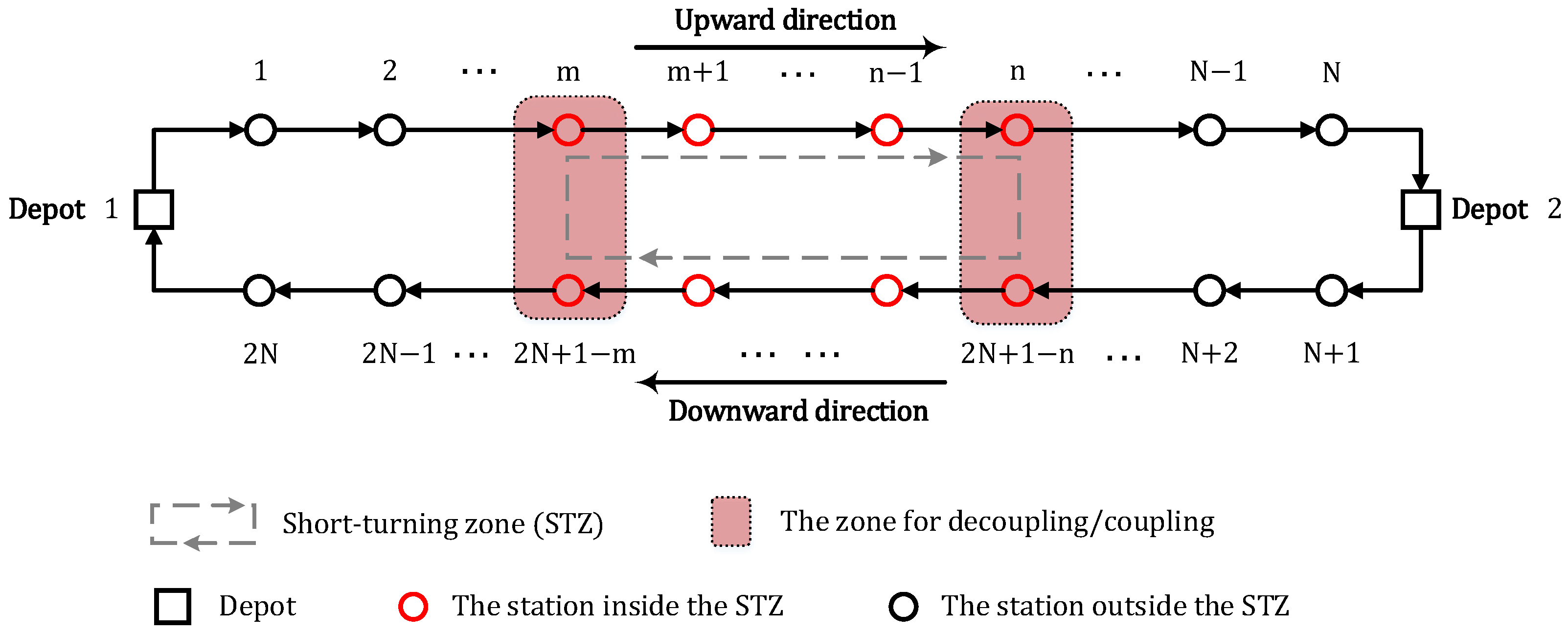
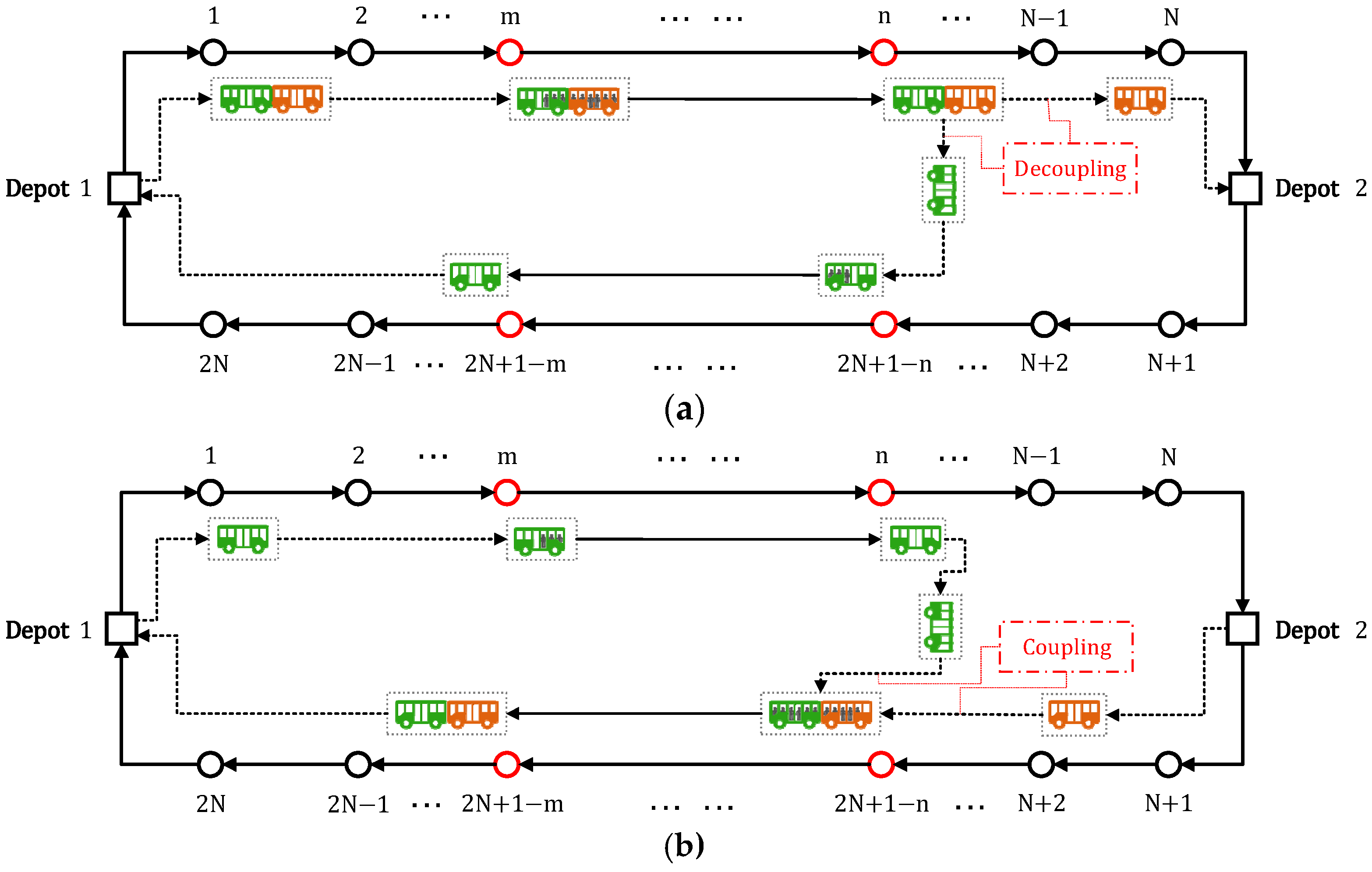
3. Problem Description

In this study, we consider a bi-directional bus route with $2N$ stations, where the direction in which the bus runs from station 1 to station $N$ is defined as the upward direction, and the direction in which it runs from station $N+1$ to $2N$ is defined as the downward direction, and the line is flanked by depots storing the modularized units, which are connected to the start and end stations in the upward and downward directions. Intermediate turnaround stops are provided in the up and down directions, with stop m and stop n in the up direction and stop $m1=2N+1-m$ and stop $n1=2N+1-n$ in the down direction, allowing transit to turnaround along the up/down direction to the down/up direction for service. Depending on the turnaround route, the MV can operate coupled in the upward direction at stop m and in the downward direction at stops $2N+1-n$, denoted by the symbol $y{c}_s$, and decoupled in the upward direction at stop n and in the downward direction at stops $2N+1-m$, denoted by the symbol $y{d}_s$. The layout of the studied line is shown in Figure 1.

We study the operation of short-turning trips based on a single full-length trip in the case of uneven distribution of passenger demand in a two-way bus route. Full-length trips serve all stops along the route, operating between the starting and ending stations in both up and down directions. Short-turning trips serve a portion of the route, operating between intermediate return stations in both up and down directions. In this operational scenario, in addition to adjusting the formation of MV at the starting station, due to the directional imbalance in passenger demand, we consider decoupling/coupling MVs at intermediate turnaround stations to meet the demand in the corresponding direction.

The decoupling and coupling operations of MVs at turnaround stations are as follows. When the downward passenger demand does not require all MUs from the upward direction to turn back, the MVs can be decoupled at the turnaround station. As shown in Figure 2a, the MVs in the upward direction are decoupled at station $n$. The decoupled green MU turns back to the opposite direction to serve passengers for the corresponding trip. The remaining orange MU deadheads back to depot 2.

When the MVs turning back in the upward direction cannot meet the passenger demand in the opposite direction, additional MUs need to be dispatched for coupling. As shown in Figure 2b, the green MU from the upward direction turns back to station $2N+1-n$ in the opposite direction. Simultaneously, depot 2 dispatches an orange MU to the same station through deadheading. After the green and orange MU are coupled into a single MV, they jointly serve passengers for the corresponding trip in the downward direction.

Here, we only analyze the decoupling/coupling operation of MVs from the upward direction to the downward direction at the turnaround station under the short-turning strategy, and the same for the downward direction.

Based on the aforementioned description, each trip determines whether to operate in full-length service mode or short-turning service mode, as well as its departure capacity, according to the passenger demand at each station. MVs operating on short-turning routes decide on decoupling/coupling schemes at turnaround stations based on the unbalanced passenger demand in both directions of the route. The goal is to better match demand and capacity supply within the public transportation system, providing more targeted services for unevenly distributed passenger demands along the route, thereby reducing both passenger waiting time costs and public transit operational costs. To establish the mathematical model for the problem under study, we make the following assumptions:

Assumption 1: Passenger arrival rates at each station remain constant during peak periods; Assumption 2: The MUs stored in the depot setup at the start and end stations are sufficient; Assumption 3: Inter-station running times as well as station dwell times are predetermined; Assumption 4: Passengers will always choose the trip whose origin and destination are within the service area without transferring; Assumption 5: All passengers waiting to board a trip are assumed to have equal boarding opportunities [30]; Assumption 6: MV decoupling/coupling time is negligible.

4. Model Formulation and Solution

4.1. Notation

For the reader’s convenience, all symbols used in the equations are tabulated in

Table 1. Notation table.

Symbol	Description
Sets
$T$	$\mathrm{Set} \mathrm{of} \mathrm{discreted} \mathrm{time} \mathrm{intervals}, \mathrm{i}.\mathrm{e}., T=\left\{1,2,\dots ,I\right\}$
$S^u,S^d$	Sets of stations in the up and down direction, $\mathrm{i}.\mathrm{e}., S^u=\left\{1,2,\dots ,N\right\},S^d=\left\{N+1,N+2,\dots ,2N\right\}$
$S$	Set of all stations, $\mathrm{i}.\mathrm{e}., S=S^u\cup S^d$
$K^u,K^d$	Sets of trips in the up and down direction, $\mathrm{i}.\mathrm{e}., K^u=\left\{1,2,\dots ,K_1\right\},K^d=\left\{K_1+1,K_1+2,\dots ,K_2\right\}$
$K$	Set of all trips, $\mathrm{i}.\mathrm{e}., K=K^u\cup K^d$
Parameters
$c$	Capacity of individual MU
$n_{\max }$	Maximum number of MUs in a MV
${\varphi }_{s{s}^{+}}$	Passenger arrival rate from station $s$ to stop $s^{+}$
$f_i$	Operational cost of a MV to complete one trip
$f_s$	Fixed operating cost for a MV
$f_v$	Marginal operating cost for a MV
$h_{\min },h_{\max }$	Maximum and minimum headway
${\tau }_{ks}$	Dwell time of MV on trip $k$ at station $s$
$t{r}_s$	Running time of MV from station $s$ to station $s+1$
$\gamma$	Passenger waiting time cost per unit time
$M$	a large value
$tr{n}_{\min },tr{n}_{\max }$	Maximum and minimum turnaround time
$s{s}_s,f{s}_s$	Stopping station for short-turning trips, full-length trips. 1 if stopping, 0 otherwise
$y{d}_s,y{c}_s$	MV decoupling and coupling stations. 1 if yes, otherwise 0
${\omega }_1,{\omega }_2$	Weights in the objective function
Decision variables
$t{n}_{kl}$	Number of MUs for MV turnaround on trip $k$ to trip $l$ in the opposite direction
$c{p}_k$	Number of MUs provided by the depot for coupling to trip $k$
$v_{kl}$	Binary variable that equals 1 if the MV on trip $k$ turnaround to trip $l$, and 0 otherwise
${\lambda }_k$	Binary variable that equals 1 if trip $k$ is a short-turning trip, and $0$ otherwise
$h_k$	Headway of trip $k$ at the initial station
Dependent variables
$i_{ks}$	Number of MUs of the MV on trip $k$ at station $s$
$dc{p}_k$	Number of MUs decoupled from the MV on trip $k$ at the designated station
$ot{n}_l$	Number of MUs provided to trip $l$ by the turnaround after decoupling from MV of the opposite direction trip
${\alpha }_k$	Binary variable that equals 1 if the MV on a trip in the opposite direction turnaround to trip $k$, and 0 otherwise
${\beta }_k$	Binary variable that equals 1 if the MV on trip $k$ turnaround to the opposite direction, and $0$ otherwise
${\mu }_{ks}$	Binary variable that equals 1 if trip $k$ stops at station $s$
$r_{ks{s}^{+}}$	Number of passengers arriving at station $s$ and destined for station $s^{+}$ between trip $k-1$ and trip $k$
$w_{ks{s}^{+}}$	Number of passengers arriving at station $s$ with destination station $s^{+}$ in the interval between trip $k-1$ and trip $k$
$w_{ks{s}^{+}}^g$	Number of passengers actually waiting at station $s$ for the MV of trip $k$ with destination station $s^{+}$
${\rho }_{ks{s}^{+}}$	Binary variable that equals 1 If trip $k$ stops at both station $s$ and $s^{+}$, and 0 otherwise
$m_{ks{s}^{+}}$	Number of passengers boarding MV of trip $k$ at station $s$ with destination station $s^{+}$
$l_{ks{s}^{+}}$	Number of passengers failing to board the MV on trip $k$ at station $s$ with destination station $s^{+}$
$a_{ks}$	Number of passengers arriving at station $s$ between trip $k-1$ and trip $k$
$w_{ks}$	Number of passengers waiting for the MV on trip $k$ at station $s$
$w_{ks}^g$	Number of passengers actually waiting at station $s$ for the MV of trip $k$
$g_{ks}$	Number of passengers boarding the MV on trip $k$ at station $s$
$o_{ks}$	Number of passengers alighting from the MV on trip $k$ at station $s$
$b_{ks}$	Number of passengers on board the MV on trip $k$ before arriving at station $s$
$l_{ks}$	Number of passengers failing to board the MV on trip $k$ at station $s$
$pro{p}_{ks{s}^{+}}$	Proportion of passengers boarding trip $k$ from station $s$ to station $s^{+}$
$ar{r}_{ks}$	Arrival time of the MV on trip $k$ at station $s$
$de{p}_{ks}$	Departure time of the MV on trip $k$ from station $s$
${\zeta }_{ks},{\xi }_{ks}$	Binary variables used for linearization

.

4.2. Constraints

4.2.1. Vehicle Operation Constraints

Due to the adoption of the short-turning strategy, the serviced stops differ between the short-turning and full-length service modes within the study period. As described in the line layout in Figure 1, it has been explained that the full-length service mode provides service at all stations from Station 1 to Station $N$ in the upstream direction and from Station $N+1$ to Station $2N$ in the downstream direction, represented by $f{s}_s$. In contrast, the short-turning service mode provides service only at stations from Station m to Station n in the upstream direction and from Station $2N+1-n$ to Station $2N+1-m$ in the downstream direction, represented by $s{s}_s$. Then, the formula for whether trip k stops at station s for service is expressed as follows:

$${\mu }_{ks}={\lambda }_k\times s{s}_s+\left(1-{\lambda }_k\right)\times f{s}_s,\forall s\in S,k\in K$$

(1)

In order to avoid long waiting times for passengers at some stations, one of the two consecutive trips in each direction must be a full-length trip, subject to the following constraint:

$${\lambda }_{k-1}+{\lambda }_k\le 1,\forall k\in K^u/\left\{1\right\}\hspace{0.17em}\hspace{0.33em}or\hspace{0.33em}\hspace{0.17em}k\in K^d/\left\{K_1+1\right\}\hspace{0.17em}$$

(2)

Then, the specific operation process of the bus is modeled, including the arrival and departure times of each trip on the line, and the departure interval between two adjacent trips. The arrival time of trip $k$ at stop $s$ is determined by adding the departure time of trip $k$ at stop $s-1$ to the running time from stop $s-1$ to stop $s$. The departure time of trip $k$ at stop $s$ is the arrival time of trip $k$ at that stop plus the dwell time, expressed as follows:

$$ar{r}_{ks}=de{p}_{k,s-1}+t{r}_s,\forall s\in S^u/\left\{1\right\},k\in K^u\hspace{0.17em}or\hspace{0.17em}\hspace{0.17em}\forall s\in S^d/\{N+1\},k\in K^d$$

(3)

$$de{p}_{ks}=ar{r}_{ks}+{\tau }_{ks},\forall s\in S,k\in K$$

(4)

It should be noted that, in order to facilitate modeling, the virtual arrival time and departure time are defined for the stations outside the short-turning interval of the short-turning trip, which also meet the constraints (3) and (4).

In addition, to ensure the quality of service, we require that the last trips on both directions of the line are full-length trips, and that the difference between their departure time at the first station and the end time of the study range cannot exceed the maximum departure interval, satisfying the following constraints:

$$I-h_{\max }\le de{p}_{K_1,1},de{p}_{K_2,N+1}\le I$$

(5)

$${\lambda }_{K_1}={\lambda }_{K_2}=0$$

(6)

In addition, to ensure the quality of service, we require that the last trip on both directions of the line be a full-length trip and both depart from the first station at the end time of the study horizon, satisfying the following constraints:

The departure interval between trip $k-1$ and trip $k$ is the difference between their departure times at the starting station, and the interval corresponding to the first trip in both directions is the difference between their departure times at the starting station and the start time of the study period, and the departure interval of each trip in both directions at the starting station is required to satisfy the minimum and maximum interval constraints, which are expressed as follows:

$$h_k=de{p}_{ks},\forall k\in 1,s=1\hspace{0.33em}\hspace{0.33em}or\hspace{0.33em}\hspace{0.33em}\forall k\in K_1+1,s=N+1$$

(7)

$$h_k=de{p}_{ks}-de{p}_{k-1,s},\forall k\in K^u/\left\{1\right\},s=1\hspace{0.33em}\hspace{0.33em}or\hspace{0.33em}\hspace{0.17em}\forall k\in K^d/\{K_1+1\},s=N+1$$

(8)

$$h_{\min }\le h_k\le h_{\max }$$

(9)

4.2.2. Turnaround Constraints

Turnaround operations allow short-turning trips to serve trips in the opposite direction after a turnaround at a turnaround station, which means that both the trips before and after the turnaround are short-turning trips. The constraints are as follows:

$$2\times v_{kl}\le {\lambda }_k+{\lambda }_l,\forall k\in K^u,l\in K^d$$

(10)

$$2\times v_{kl}\le {\lambda }_k+{\lambda }_l,\forall k\in K^d,l\in K^u$$

(11)

If trip $k$ is a short-turning trip, the trip may return directly to the terminal depot after completing this service, or it may turn around to continue service in the opposite direction. We use the symbols ${\alpha }_k$ and ${\beta }_k$ to denote the above; if ${\alpha }_k=1$, it means that the MV of trip $k$ is provided by the trip $l$ in the opposite direction after the turnaround; if ${\beta }_k=1$, it means that trip $k$ will not return to the depot of the terminal after finishing this service, but turnaround to the opposite direction to continue the service of trip $l$, which is denoted as follows:

$${\alpha }_k={\displaystyle \sum _{l\in K^d}{v}_{lk},}\forall k\in K^u$$

(12)

$${\alpha }_k={\displaystyle \sum _{l\in K^u}{v}_{lk},}\forall k\in K^d$$

(13)

$${\beta }_k={\displaystyle \sum _{l\in K^d}{v}_{kl},}\forall k\in K^u$$

(14)

$${\beta }_k={\displaystyle \sum _{l\in K^u}{v}_{kl},}\forall k\in K^d$$

(15)

$${\alpha }_k+{\beta }_k=2\times v_{kl},if\hspace{0.17em}{v}_{kl}=1,\forall k\in K^u,l\in K^d$$

(16)

$${\alpha }_k+{\beta }_k=2\times v_{kl},if\hspace{0.17em}{v}_{kl}=1,\forall k\in K^d,l\in K^u$$

(17)

When a short-turning trip completes its service in the up/down direction and turns back to continue service in the opposite direction (when $v_{kl}=1$), the turnaround time must meet the minimum and maximum turnaround time constraints. That is, the difference between the departure time of the up-direction short-turning trip $k$ from turnaround station $n$ and the arrival time of the down-direction short-turning trip $l$ at station $2N+1-n$ should satisfy the minimum and maximum time constraints. Similarly, the difference between the departure time of the down-direction short-turning trip $k$ from turnaround station $2N+1-m$ and the arrival time of the up-direction short-turning trip $l$ at station $m$ should satisfy the minimum and maximum time constraints. This can be expressed as follows:

$$tr{n}_{\min }\le ar{r}_{l,2N+1-n}-de{p}_{km}\le tr{n}_{\max },\hspace{0.33em}\hspace{0.33em}if\hspace{0.17em}\hspace{0.17em}{v}_{kl}=1,\forall k\in K^u,l\in K^d$$

(18)

$$tr{n}_{\min }\le ar{r}_{lm}-de{p}_{k,2N+1-m}\le tr{n}_{\max },\hspace{0.33em}\hspace{0.33em}if\hspace{0.17em}\hspace{0.17em}{v}_{kl}=1,\forall k\in K^d,l\in K^u$$

(19)

4.2.3. Decoupling/Coupling Operation Constraints

For each trip on a bi-directional route, we need to determine the specific number of MUs of MV at each station for each trip. The number of MUs of the MV at each trip from the first station is the variable to be decided, and by default it has been decoupled/coupled before the departure at the depot.

According to the description in Section 3, MVs can only be operated uncoupled/coupled at designated turnaround sites. The number of decoupled/coupled MUs is determined by the following constraints:

$$dc{p}_k={\displaystyle \sum _{l\in K^d}t{n}_{kl}},\forall k\in K^u$$

(20)

$$dc{p}_k={\displaystyle \sum _{l\in K^u}t{n}_{kl}},\forall k\in K^d$$

(21)

$$ot{n}_l={\displaystyle \sum _{k\in K^d}t{n}_{kl}},\forall l\in K^u$$

(22)

$$ot{n}_l={\displaystyle \sum _{k\in K^u}t{n}_{kl}},\forall l\in K^d$$

(23)

$$t{n}_{kl}\le v_{kl}\times i_{k,n-1},\forall k\in K^u,l\in K^d$$

(24)

$$t{n}_{kl}\le v_{kl}\times i_{k,2N-m},\forall k\in K^d,l\in K^u$$

(25)

$$c{p}_k\le {\alpha }_k\times \left(n_{\max }-ot{n}_k\right),\forall k\in K$$

(26)

We use the symbol $t{n}_{kl}$ to represent the number of MUs of MV that are turnaround from the up/down direction short-turning trip $k$ to the opposite direction short-turning trip, that is, the number of decoupled MUs $dc{p}_k$ of short-turning trip $k$ (calculated through Equations (20) and (21)); it is also the number of MUs $ot{n}_l$ provided by short-turning trip $l$ after being decoupled and turned over from the MV of the opposite direction short-turning trip $k$ (calculated through Equations (22) and (23)). Constraints (24) and (25) ensure that the number of MUs turnaround from the up/down direction short-turning trip $k$ to the opposite direction short-turning trip $l$ at the turnaround station does not exceed the number of MUs at the station immediately preceding the turnaround station. Constraint (26) restricts the number of MUs provided by the depot for coupling to short-turning trip $k$ to not exceed the difference between the maximum allowable number of MUs for coupling $n_{\max }$ and the number of MUs provided by the short-turning trip $l$ after being turnaround from the opposite direction $ot{n}_k$.

Then, the number of MUs of MVs at each station of the bi-directional route is updated according to the following formula:

$$i_{ks}=i_{k,s-1}-{\beta }_k\times dc{p}_k\times y{d}_s+{\alpha }_k\times \left(ot{n}_k+c{p}_k\right)\times y{c}_s,\forall s\in S/\left\{1\right\},k\in K^u$$

(27)

$$i_{ks}=i_{k,s-1}-{\beta }_k\times dc{p}_k\times y{d}_s+{\alpha }_k\times \left(ot{n}_k+c{p}_k\right)\times y{c}_s,\forall s\in S/\left\{N+1\right\},k\in K^d$$

(28)

When the up/down direction short-turning trip $k$ is provided by the MV of a short-turning trip from the opposite direction after turning back (i.e., when ${\alpha }_k=1$), the number of MUs of short-turning trip $l$ at the initial station is 0, which can be represented as follows:

$$i_{k1}=0,\hspace{0.33em}if\hspace{0.33em}\hspace{0.33em}{\alpha }_k=1,\forall k\in K^u$$

(29)

$$i_{k,N+1}=0,\hspace{0.33em}if\hspace{0.33em}\hspace{0.33em}{\alpha }_k=1,\forall k\in K^d$$

(30)

4.2.4. Passenger Flow Dynamic Evolution Constraints

The dynamic changes in passenger flow at various stations are related to the operation schedule and the MV capacity. We model the passenger flow situation of each trip at each station.

We first analyze in detail the passengers arriving at station $s$ and with destination station $s^{+}$. The formula for the number of passengers arriving at station $s$ and with destination station $s^{+}$ during the departure interval between trip $k-1$ and trip $k$ is as follows:

$$r_{ks{s}^{+}}=\left\{\begin{array}{c}{\varphi }_{s{s}^{+}}\times de{p}_{ks},\hspace{0.33em}\hspace{0.33em}\hspace{0.33em}\hspace{0.33em}\hspace{0.33em}\hspace{0.33em}\hspace{0.33em}if\hspace{0.33em}\hspace{0.33em}k=1,K_1+1\hfill \\ {\varphi }_{s{s}^{+}}\times (de{p}_{ks}-de{p}_{k-1,s}),otherwise\hfill \end{array}\right.,\forall k\in K,s,s^{+}\in S,s<s^{+}$$

(31)

The number of passengers waiting at station $s$ for trip $k$ with a destination of station $s^{+}$, consists of two parts: the number of passengers arriving at station $s$ during the interval between trip $k-1$ and trip $k$, and the number of passengers who were unable to board the previous trip $k-1$, expressed as follows:

$$w_{ks{s}^{+}}=\left\{\begin{array}{c}{r}_{ks{s}^{+}},\hspace{0.33em}\hspace{0.33em}\hspace{0.33em}\hspace{0.33em}\hspace{0.33em}\hspace{0.33em}\hspace{0.33em}if\hspace{0.33em}\hspace{0.33em}k=1,K_1+1\hfill \\ r_{ks{s}^{+}}-l_{k-1,s{s}^{+}},otherwise\hfill \end{array}\right.,\forall k\in K,s,s^{+}\in S,s<s^{+}$$

(32)

Based on Assumption 4, passengers will choose the trip $k$ whose departure and destination stops are both within the service interval of the trip, therefore, the number of passengers actually waiting to take trip $k$ in the interval between trip $k-1$ and trip $k$ is calculated by Equation (33). The ${\rho }_{ks{s}^{+}}$ is used to indicate whether trip $k$ serves both station $s$ and station $s^{+}$, satisfying the constraint (34).

$$w_{ks{s}^{+}}^g=w_{ks{s}^{+}}\times {\rho }_{ks{s}^{+}},\forall k\in K,s,s^{+}\in S,s<s^{+}$$

(33)

$$2\times {\rho }_{ks{s}^{+}}\le {\mu }_{ks}+{\mu }_{k{s}^{+}},\forall k\in K,s,s^{+}\in S,s<s^{+}$$

(34)

Based on Assumption 5, where passengers actually waiting for trip $k$ at station $s$ have an equal chance of boarding the vehicle, the formula for calculating the number of passengers whose destination station is $s^{+}$ and who successfully take trip $k$ is as follows:

$$m_{ks{s}^{+}}={\displaystyle \frac{w_{ks{s}^{+}}^g}{w_{ks}^g}}\times g_{ks},\forall k\in K,s,s^{+}\in S,s<s^{+}$$

(35)

Due to limited vehicle capacity or short-turning strategies, some passengers may not be able to board the vehicle, as indicated below:

$$l_{ks{s}^{+}}=w_{ks{s}^{+}}-m_{ks{s}^{+}},\forall k\in K,s,s^{+}\in S,s<s^{+}$$

(36)

Then, we performed an overall analysis of the number of passengers at station $s$. We calculated separately: the number of passengers arriving at station $s$ in the time interval between trip $k-1$ and trip $k$, the number of passengers actually waiting to take trip $k$ in the time interval between trip $k-1$ and trip $k$, the number of passengers getting off at station $s$ for trip $k$, and the number of passengers failing to board trip $k$ at station $s$, expressed as follows:

$$a_{ks}=\left\{\begin{array}{c}{\displaystyle \sum _{s^{+}=s+1}^N{r}_{ks{s}^{+}}},\forall k\in K^u,s,s^{+}\in S^u,s<s^{+}\\ {\displaystyle \sum _{s^{+}=s+1}^{2N}{r}_{ks{s}^{+}}},\forall k\in K^d,s,s^{+}\in S^d,s<s^{+}\end{array}\right.$$

(37)

$$w_{ks}^g=\left\{\begin{array}{c}{\displaystyle \sum _{s^{+}=s+1}^N{w}_{ks{s}^{+}}^g},\forall k\in K^u,s,s^{+}\in S^u,s<s^{+}\\ {\displaystyle \sum _{s^{+}=s+1}^{2N}{w}_{ks{s}^{+}}^g},\forall k\in K^d,s,s^{+}\in S^d,s<s^{+}\end{array}\right.$$

(38)

$$o_{ks}=\left\{\begin{array}{c}\hspace{0.33em}\hspace{0.33em}\hspace{0.33em}0,\hspace{0.33em}\hspace{0.33em}\hspace{0.33em}\hspace{0.33em}\hspace{0.33em}\hspace{0.33em}\hspace{0.33em}\forall k\in K,s=1,I+1\\ {\displaystyle \sum _{s^{-}\in S}{m}_{k{s}^{-}s}},\forall k\in K,s^{-},s\in S,s^{-}<s\end{array}\right.$$

(39)

$$l_{ks}=\left\{\begin{array}{c}{\displaystyle \sum _{s^{+}=s+1}^N{l}_{ks{s}^{+}}},\forall k\in K^u,s,s^{+}\in S^u,s<s^{+}\\ {\displaystyle \sum _{s^{+}=s+1}^{2N}{l}_{ks{s}^{+}}},\forall k\in K^d,s,s^{+}\in S^d,s<s^{+}\end{array}\right.$$

(40)

The number of passengers boarding trip $k$ at station $s$ depends on the remaining capacity of the MV when trip $k$ arrives at the station and the number of passengers actually waiting to take trip $k$. Wherein the remaining capacity of the MV is the total capacity minus the number of passengers on board the vehicle before the arrival at the station plus the number of passengers getting off the vehicle at the station. Thus, the formula for $g_{ks}$ is as follows:

$$g_{ks}=\min \left(c\times i_{ks}-b_{ks}+o_{ks},w_{ks}^g\right),\forall k\in K,s\in S$$

(41)

The number of passengers in the vehicle when trip $k$ arrives at station $s$ is categorized into two cases by station: first, when trip $k$ arrives at the first station of a two-way route, the number of passengers in the vehicle is $0$; second, when trip $k$ arrives at other station $s$, the number of passengers in the vehicle is the number of passengers in the vehicle when trip $k$ arrives at station $s-1$ plus the number of people boarding the vehicle at station $s-1$, and then subtracting the number of people exiting the vehicle at station $s-1$, as expressed as follows:

$$b_{ks}=\left\{\begin{array}{c}\hspace{0.33em}\hspace{0.33em}\hspace{0.33em}0,\hspace{0.33em}\hspace{0.33em}\hspace{0.33em}\hspace{0.33em}\hspace{0.33em}\hspace{0.33em}\hspace{0.33em}\forall k\in K,s=1,I+1\\ b_{k,s-1}+g_{k,s-1}-o_{k,s-1},\forall k\in K,s\in S\end{array}\right.$$

(42)

4.3. Objective Functions

The objective function of the model in this paper aims to minimize the weighted sum of passenger waiting time costs and vehicle operating costs. The calculation formula is as follows:

$$\min \hspace{0.33em}Z={\omega }_1\times Z_w+{\omega }_2\times Z_v$$

(43)

In which, ${\omega }_1$ and ${\omega }_2$ represent the weight coefficients, $Z_w$ represents the cost of passenger waiting time, and $Z_v$ represents the operating cost of the vehicle. Considering the equal importance of passenger waiting time cost and vehicle operating cost in the public transportation system, in this study, the weights ${\omega }_1$ and ${\omega }_2$ are both set to 1 [22,31].

4.3.1. Passenger Waiting Time Cost

The waiting time for passengers consists of three parts: the first part is the waiting time $C_{w1}$ for passengers who arrive at each station from the start of the study period until the departure of the first trip; the second part is the waiting time $C_{w2}$ for passengers who arrive at each station between two consecutive trips; and the third part is the waiting time $C_{w3}$ for passengers who were unable to board the previous trip. Therefore, the passenger’s total waiting time cost is shown in Equation (47), which consists of the total waiting time multiplied by the passenger’s waiting time cost per unit of time $\gamma$.

$$C_{w1}={\displaystyle \sum _{s\in S^u}\frac{1}{2}\times a_{ks}}\times \left(de{p}_{1s}\right)+{\displaystyle \sum _{s\in S^d}\frac{1}{2}\times a_{kss}}\times \left(de{p}_{K_1+1,s}\right)$$

(44)

$$C_{w2}={\displaystyle \sum _{k=2}^{K_1}{\displaystyle \sum _{s\in S^u}\frac{1}{2}\times a_{ks}}\times \left(de{p}_{ks}-de{p}_{k-1,s}\right)}+{\displaystyle \sum _{k=K_1+2}^{K_2}{\displaystyle \sum _{s\in S^d}\frac{1}{2}\times a_{ks}\times }\left(de{p}_{ks}-de{p}_{k-1,s}\right)}$$

(45)

$$C_{w3}={\displaystyle \sum _{k=1}^{K_1-1}{\displaystyle \sum _{s\in S^u}\left(de{p}_{k+1,s}-de{p}_{k,s}\right)\times l_{ks}}}+{\displaystyle \sum _{k=K_1+1}^{K_2-1}{\displaystyle \sum _{s\in S^d}\left(de{p}_{k+1,s}-de{p}_{k,s}\right)\times l_{ks}}}$$

(46)

$$Z_w=\left(C_{w1}+C_{w2}+C_{w3}\right)\times \gamma$$

(47)

4.3.2. Vehicle Operating Cost

The operational costs of MVs differ from those of conventional buses. According to reference [13,14], the calculation formula for the operational cost of a MV composed of $i$ MUs is as follows:

$$f_i=f_s+f_v\times {\left(i\times c\right)}^{\sigma }$$

(48)

in which $f_s$ represents the fixed operating cost, $f_v$ represents the marginal operating cost, the parameter $\sigma (0<\sigma \le 1)$ is used to describe the economies of scale for MVs of different capacities [24], and in this study, the parameter $\sigma$ is taken as 1.

Due to the possibility of decoupling/coupling operations at the turnaround station, which may change the capacity of MVs for short-turning trips, the operating cost for a single trip is calculated by accumulating the operating costs of MVs at each station. The formula is as follows:

$$C_{v1}={\displaystyle \sum _{k\in K^u}{\displaystyle \sum _{\mathrm{s}=1}^{N-1}\frac{f_{i_{ks}}}{N-1}}}+{\displaystyle \sum _{k\in K^d}{\displaystyle \sum _{\mathrm{s}=N+1}^{2N-1}\frac{f_{i_{ks}}}{N-1}}}$$

(49)

In addition, the MUs provided by the up and down direction depot for coupling the corresponding trips also have an operating cost, which is calculated in the following formula:

$$C_{v2}={\displaystyle \sum _{k\in K^u}\left(\frac{f_{c{p}_k}}{N-1}\times \left(m-1\right)\right)}+{\displaystyle \sum _{k\in K^d}\left(\frac{f_{c{p}_k}}{N-1}\times \left(N-n\right)\right)}$$

(50)

The total operational cost of MVs is calculated using Formula (51):

$$Z_v=C_{v1}+C_{v2}$$

(51)

4.4. Model Solving

In summary, an integer nonlinear programming model is constructed with (43) as the objective function and Equations (1)–(42) as constraints. We use the commercial solver Gurobi version 12.0.0 for the solution, which requires equivalent replacement of some nonlinear and nonquadratic terms in the model.

For constraints (16) and (17), we introduce a maximal value $M$. Constraints (16) and (17) can be equivalently replaced by the following linear constraints:

$$\left\{\begin{array}{c}{\alpha }_{\mathrm{k}}+{\beta }_l\le 2+M\times \left(1-v_{kl}\right),\forall k\in K^u,l\in K^d\\ {\alpha }_{\mathrm{k}}+{\beta }_l\le 2+M\times \left(1-v_{kl}\right),\forall k\in K^d,l\in K^u\\ {\alpha }_{\mathrm{k}}+{\beta }_l\ge 2-M\times \left(1-v_{kl}\right),\forall k\in K^d,l\in K^u\\ {\alpha }_{\mathrm{k}}+{\beta }_l\le 2+M\times \left(1-v_{kl}\right),\forall k\in K^d,l\in K^u\end{array}\right.$$

(52)

For constraints (18) and (19), they can be equivalently replaced with the following linear constraints:

$$\left\{\begin{array}{c}ar{r}_{l,2N+1-n}-de{p}_{km}\ge tr{n}_{\min }-M\times \left(1-v_{kl}\right),\forall k\in K^u,l\in K^d\\ ar{r}_{l,2N+1-n}-de{p}_{km}\le tr{n}_{\max }+M\times \left(1-v_{kl}\right),\forall k\in K^u,l\in K^d\\ ar{r}_{lm}-de{p}_{k,2N+1-m}\ge tr{n}_{\min }-M\times \left(1-v_{kl}\right),\forall k\in K^d,l\in K^u\\ ar{r}_{lm}-de{p}_{k,2N+1-m}\le tr{n}_{\max }+M\times \left(1-v_{kl}\right),\forall k\in K^d,l\in K^u\end{array}\right.$$

(53)

For constraints (29) and (30), they can be equivalently transformed into the following linear constraints:

$$\left\{\begin{array}{c}{i}_{k1}\le \left(1-{\alpha }_k\right)\times M,\forall k\in K^u\\ i_{k,N+1}\le \left(1-{\alpha }_k\right)\times M,\forall k\in K^d\end{array}\right.$$

(54)

For constraint (35), we introduce the variable $pro{p}_{ks{s}^{+}}={\displaystyle \frac{w_{ks{s}^{+}}^g}{w_{ks}^g}}$, which represents the proportion of passengers waiting at station $s$ for trip $k$ with a destination of station $s$ out of all passengers waiting for trip $k$. Constraint (35) can be equivalently replaced by the following quadratic constraint:

$$\left\{\begin{array}{c}{w}_{ks{s}^{+}}^g=pro{p}_{ks{s}^{+}}\times w_{ks}^g\\ m_{ks{s}^{+}}=pro{p}_{ks{s}^{+}}\times g_{ks}\end{array}\right.$$

(55)

For constraint (41), we introduce binary variables ${\zeta }_{ks}$ and ${\xi }_{ks}$ to linearize it, and formulate the following set of linear constraints to replace it:

$$\left\{\begin{array}{c}\begin{array}{c}{g}_{ks}\le c\times i_{ks}-b_{ks}+o_{ks}\\ g_{ks}\ge \left(c\times i_{ks}-b_{ks}+o_{ks}\right)-M\times {\zeta }_{ks}\end{array}\\ \begin{array}{c}{g}_{ks}\le w_{ks}^g\\ g_{ks}\ge w_{ks}^g-M\times {\xi }_{ks}\\ {\zeta }_{ks}+{\xi }_{ks}\ge 1\end{array}\end{array}\right.,\forall k\in K,s\in S$$

(56)

In the process of solving the model, the simulation was run on a computer with hardware environment of Intel (R) Core (TM) i7-9750HF CPU @ 2.60GHz and 8GB RAM. The software environment was Windows 10, and the program was scripted in Python 3.12 to interface with the Gurobi version 12.0.0 for the model’s resolution.

5. Numerical Studies

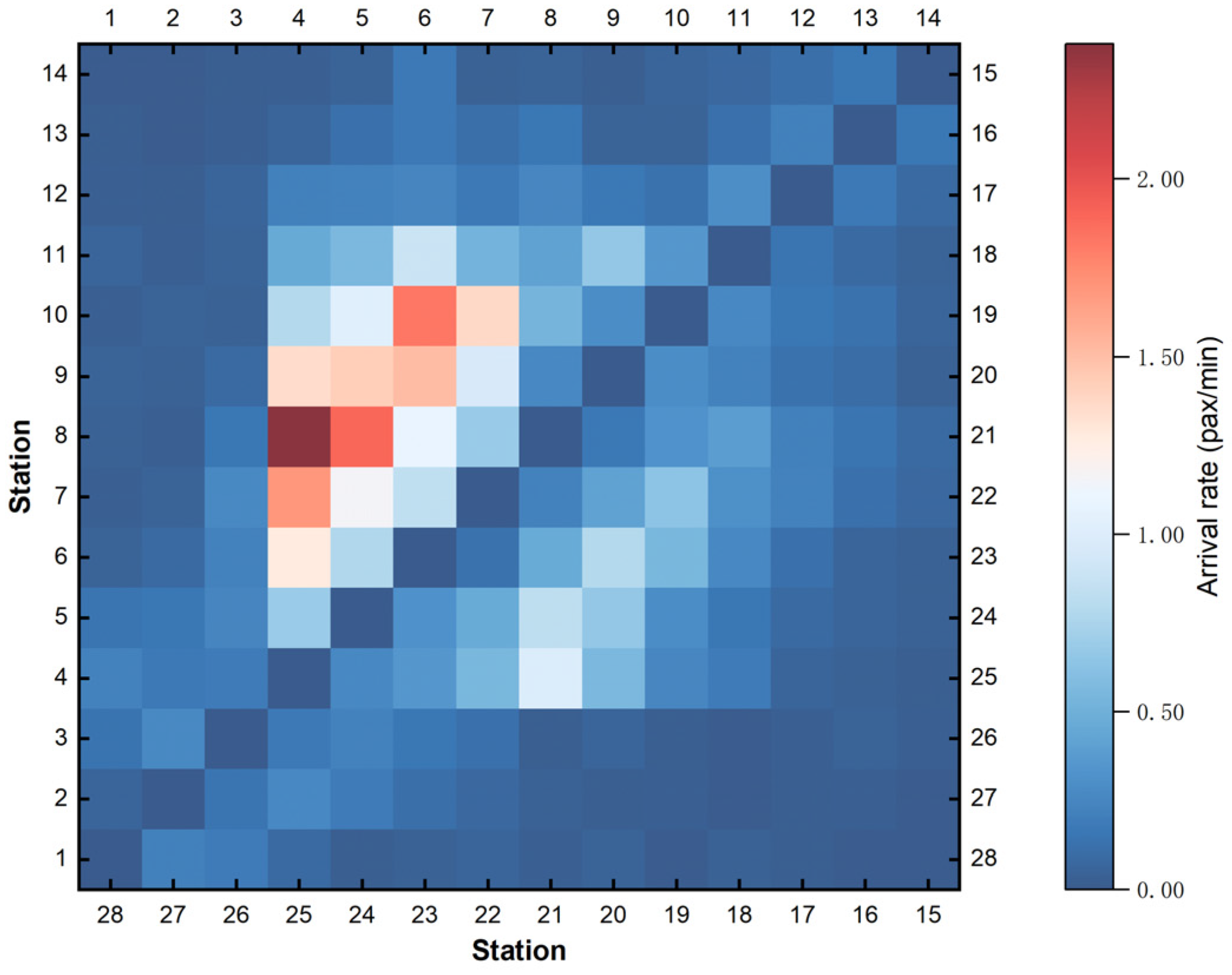
5.1. Basic Data

This paper simulates the operation of public transportation services with uneven passenger demand to test the effectiveness of the proposed model. A bidirectional bus route with 14 stations in each upward and downward direction is considered, and the study period is from 7:30 to 9:00 on weekdays during the morning peak hours, which is a 90-min time horizon with a time granularity of 1 min, i.e., $t=\left[0,90\min \right]$. There are $23$ trips in both the up and down directions, and the running time between two consecutive stations is shown in

Table 2. Running time between two consecutive stations.

Stations	Running Time (min)	Stations	Running Time (min)	Stations	Running Time (min)	Stations	Running Time (min)
1–2	2	8–9	3	15–16	2	22–23	2
2–3	2	9–10	2	16–17	2	23–24	2
3–4	2	10–11	2	17–18	3	24–25	3
4–5	3	11–12	3	18–19	2	25–26	2
5–6	2	12–13	2	19–20	2	26–27	2
6–7	2	13–14	2	20–21	3	27–28	2
7–8	2			21–22	2

. The dwell time at each station is set to 1 min. The minimum and maximum headway times for departures from the initial station are $h_{\min }=2 \min$ and $h_{\max }=5 \min$, respectively. The minimum and maximum turnaround times for short-turning trips are $tr{n}_{\min }=1 \min$ and $tr{n}_{\max }=5 \min$, respectively. Figure 3 represents the inter-station Origin–Destination passenger arrival rates for the bidirectional route, which is characterized by a clear station imbalance and directional imbalance. Based on the bidirectional passenger demand along the route, Stations 4 and 11 are selected as the turnaround stations for short-turning trips in the up direction, correspondingly, Stations 18 and 25 are selected as the turnaround stations for short-turning trips in the down direction. According to the data in the literature [22,29,32], the capacity of a single MU is set to $c=15$ passengers per MU, and the maximum number of MUs that a MV can consist of is $n_{\max }=5$. The cost of waiting time per passenger per minute is set to $w=0.8 \$/\min$, the fixed operating cost of a MV is set to $f_s=1.912 \$/\min$, and the marginal operating cost is set to $f_v=0.59 \$/\min$.

5.2. Optimization Results and Analysis

We used Gurobi version 12.0.0 to solve the proposed model and obtained the optimized MVs formation and timetable as shown in Figure 4. In the figure, solid lines indicate that the MV will stop at the connected stations to provide service, while dashed lines indicate that the MV is deadheading. The different colors of the lines correspond to the number of MUs that constitute the MV. If a line contains both solid and dashed segments, it represents a short-turning trip; if a line is entirely solid, it represents a full-length trip. U-shaped lines indicate that the MV decouples its MUs at the turnaround station and turnarounds them to the opposite direction, while the remaining MUs deadhead back to the depot. Arcs represent the MUs provided by the depot through deadheading to short-turning trip.

As can be seen in the figure, the short-turning strategy is utilized to alleviate the high passenger flow at the intermediate stations of the line during the peak period. The difference in passenger demand in both directions of the line leads to the decoupling/coupling operation of the MVs. Due to high passenger demand in the upstream direction, the number of MUs in the MV departing from the first station is greater; similarly, due to lower passenger demand in the downstream direction, the number of MUs in the MV departing from the first station is fewer. When the MV of the short-turning trips in the upstream direction are turned around, some MUs are decoupled to the downstream direction, while the remaining MUs deadhead back to the depot. When the MV of the short-turning trips in the downstream direction are turned around, the MUs provided to the upstream direction are not sufficient to meet the high passenger demand, hence a certain number of MUs from the depot deadhead to the turnaround station for coupling.

To further increase the visibility of the decoupling/coupling operation of MVs,

Table 3. Number of decoupled MUs (turnaround to opposite direction).

Trips	Numbers	Trips	Numbers
3→34	2	25→10	1
6→36	1	27→12	2
8→38	2	29→14	1
12→42	1	32→16	2
14→44	2	36→21	1

below shows the number of MUs decoupled from the MV and the specific trips of the turnaround, and

Table 4. Number of MUs to be coupled (from depot to turnaround station by deadheading).

Depot-Trip	Numbers	Depot-Trip	Numbers
Depot1→10	3	Depot1→16	2
Depot1→12	2	Depot1→21	3
Depot1→14	3

below shows the number of MUs supplied by the depot and the corresponding specific trips. Here, the vehicle operating cost corresponding to the modular units provided by the depot and deadheading to the turnaround station is 229.51 $, while the vehicle operating cost corresponding to all the trips on the two-way line is 2074.95 $.

In order to verify the validity of the proposed model, the short-turning strategy combined with MVs (ST+MV) is compared with two other schemes, namely the full-length strategy combined with MVs (FT+MV) and the full-length strategy combined with conventional buses (FT+NB) [27]. The FT+MV scheme requires MVs to serve all stations on the line, and MVs are only allowed to flexibly change capacity at the starting stations of the two-way line. The FT+NB scheme requires conventional buses to serve all stations on the line, and conventional buses can accommodate 45 passengers; that is, MVs composed of three MUs. The total cost, passenger waiting time cost, and vehicle operating cost of the three schemes are shown in Figure 5. It can be seen that the passenger waiting time cost accounts for a relatively high proportion of the total cost. In addition, compared with the other two schemes, the model proposed in this paper has certain advantages in reducing the total system cost.

To further increase the visibility of the performance differences among different schemes, Figure 6 provides a detailed comparison of the results of the three schemes. In Figure 6, the red arrow indicates the percentage decrease compared to the other scheme, while the green arrow indicates the percentage increase. As shown in Figure 6a, compared with the traditional full-length strategy combined with conventional buses (FT+NB), the model proposed in this paper can reduce the total system cost by about 19.59%. The difference is mainly caused by the passenger waiting time cost. This is because conventional buses always operate at a fixed capacity at all stations on the two-way line, and cannot meet the high demand direction of local large passenger flow during peak hours, resulting in empty running and too many passengers staying, which increases the passenger waiting time cost. The short-turning strategy can relieve the large passenger flow at the middle stations of the line, and MVs can dynamically adjust the capacity by decoupling/coupling operations to meet the passenger flow demand in different directions, which can provide higher matching transport capacity with passenger flow demand. Although the combined large-capacity MVs make the vehicle operating cost slightly higher, it also reduces the passenger waiting time cost by about 29.99%.

As shown in Figure 6b, compared with the full-length strategy combined with MVs (FT+MV), the model proposed in this paper can reduce the total system cost by about 14.65%. Since the full-length strategy combined with MVs only allows MVs to adjust the capacity at the starting stations of the two-way line, and serves all stations on the line. Therefore, it cannot effectively relieve the large passenger flow at local stations on the line, and will lead to a longer operating time of MVs. The model proposed in this paper combines the short-turning strategy, in addition to adjusting the capacity at the starting stations of the line, it also considers decoupling/coupling operations at the turnaround stations to adapt to the unbalanced passenger flow demand. Under the condition of accurately matching transport capacity for unbalanced passenger flow demand, it effectively reduces the operating cost of MVs, reducing the passenger waiting time cost and vehicle operating cost by about 17.9% and 8.11%, respectively.

In addition, we compared the results of the full-length strategy combined with MVs (FT+MV) and the traditional full-length strategy combined with conventional buses (FT+NB), as shown in Figure 6c. Since MVs can flexibly adjust the capacity at the starting stations of the two-way line, compared with conventional buses with fixed capacity, they can still adapt to the unbalanced passenger flow demand, reducing the total system cost by about 5.79%.

After the above comparison, it is found that in the face of too much passenger flow demand at local stations during peak hours and the difference between two-way lines, using the short-turning strategy combined with MVs can minimize the total system cost, which proves the effectiveness of the proposed model.

6. Conclusions

In this paper, we investigate the optimization of public transportation services by employing short-turning strategies combined with the decoupling/coupling operations of MVs. To achieve an effective match between system capacity and passenger demand during peak hours, short-turning strategies are utilized to alleviate the heavy passenger flow in specific line sections. The decoupling/coupling operations of MVs at turnaround stations can address the directional imbalance of passenger flow on bidirectional lines. The MUs of MVs are stored/provided by the depot through deadheading. By simultaneously considering the departure intervals of each trip, the number of MUs, turnaround schemes, and decoupling/coupling schemes, we formulated an integer nonlinear programming model to improve the match between capacity and demand in urban public transportation systems, thereby minimizing passenger waiting time costs and vehicle operating costs. In order to solve the model, we processed some of the nonlinear and non-quadratic terms in the model with equivalent transformations, which were then solved by the commercial solver Gurobi version 12.0.0. The numerical studies show that, compared with the traditional full-length strategy combined with conventional bus schemes, the model proposed in this paper can reduce the total system cost by about 19.59%. It can achieve precise matching between passenger demand and transport capacity, thereby reducing the passenger waiting time cost by about 29.99%, effectively alleviating the problem of passenger congestion and improving the service level of the public transportation system. Compared with the full-length strategy combined with MVs, the model in this study can also reduce the total system cost by about 14.65%.

However, there are some limitations to this work. We assumed that the dwell times of MVs at stations and the travel times between stations are fixed, whereas in reality, these times may dynamically vary due to factors such as passenger boarding and alighting speeds, traffic congestion, etc. In future research, these uncertainty factors can be taken into account. Since this paper only considers a single bus route, in further research, we hope to extend the model to large-scale traffic networks with multiple bus routes. Additionally, when passengers choose which trip to ride, they may first opt for short-turning trips and then transfer to full-length trips to reach their destination. Therefore, studying passenger trip choice behavior is also an interesting topic for research.

References

1. Bi, H.; Zhang, S.; Lu, F. Analysis of Decoupling Effects and Influence Factors in Transportation: Evidence from Guangdong Province, China. ISPRS Int. J. Geo-Inf. 2024, 13, 404. [Google Scholar] [CrossRef]
2. Abuaisha, A.; Abu-Eisheh, S. Optimization of Urban Public Transportation Considering the Modal Fleet Size: A Case Study from Palestine. Sustainability 2023, 15, 6924. [Google Scholar] [CrossRef]
3. Luan, X.; Eikenbroek, O.A.L.; Corman, F.; van Berkum, E.C. Passenger social rerouting strategies in capacitated public transport systems. Transp. Res. E Logist. Transp. Rev. 2024, 188, 103598. [Google Scholar] [CrossRef]
4. Li, X.; An, X.; Zhang, B. Minimizing passenger waiting time in the multi-route bus fleet allocation problem through distributionally robust optimization and reinforcement learning. Comput. Oper. Res. 2024, 164, 106568. [Google Scholar] [CrossRef]
5. Wu, M.; Yu, C.; Ma, W.; An, K.; Zhong, Z. Joint optimization of timetabling, vehicle scheduling, and ride-matching in a flexible multi-type shuttle bus system. Transp. Res. Part C Emerg. Technol. 2022, 139, 103657. [Google Scholar] [CrossRef]
6. Xue, H.; Jia, L.; Li, J.; Guo, J. Jointly optimized demand-oriented train timetable and passenger flow control strategy for a congested subway line under a short-turning operation pattern. Physica A 2022, 593, 126957. [Google Scholar] [CrossRef]
7. Khan, Z.S.; He, W.; Menéndez, M. Application of modular vehicle technology to mitigate bus bunching. Transp. Res. Part C Emerg. Technol. 2023, 146, 103953. [Google Scholar] [CrossRef]
8. Tang, L.; Ariano, A.D.; Xu, X.; Li, Y.; Ding, X.; Samà, M. Scheduling local and express trains in suburban rail transit lines: Mixed–integer nonlinear programming and adaptive genetic algorithm. Comput. Oper. Res. 2021, 135, 105436. [Google Scholar] [CrossRef]
9. Yuan, J.; Gao, Y.; Li, S.; Liu, P.; Yang, L. Integrated optimization of train timetable, rolling stock assignment and short-turning strategy for a metro line. Eur. J. Oper. Res. 2022, 301, 855–874. [Google Scholar] [CrossRef]
10. Gong, C.; Luan, X.; Yang, L.; Qi, J.; Corman, F. Integrated optimization of train timetabling and rolling stock circulation problem with flexible short-turning and energy-saving strategies. Transp. Res. Part C Emerg. Technol. 2024, 166, 104756. [Google Scholar] [CrossRef]
11. Wang, F.; Wang, P.; Zhu, Z.; Xu, R.; Pan, H.; Bešinovi, N. Robust optimization of train timetables with short-length and full-length services considering uncertain passenger volume and service choice behavior. Transp. Res. Part C Emerg. Technol. 2024, 169, 104855. [Google Scholar] [CrossRef]
12. Shi, X.; Li, X. Operations design of modular vehicles on an oversaturated corridor with first-in, first-out passenger queueing. Transp. Sci. 2021, 55, 1187–1205. [Google Scholar] [CrossRef]
13. Chen, Z.; Li, X.; Qu, X. A continuous model for designing corridor systems with modular autonomous vehicles enabling station-wise docking. Transp. Sci. 2022, 56, 1–30. [Google Scholar] [CrossRef]
14. Tian, Q.; Lin, Y.H.; Wang, D.Z.W.; Yang, K. Toward real-time operations of modular-vehicle transit services: From rolling horizon control to learning-based approach. Transp. Res. Part C Emerg. Technol. 2025, 170, 104938. [Google Scholar] [CrossRef]
15. Zhang, H.; Zhao, S.; Liu, H.; Liang, S. Design of integrated limited-stop and short-turn services for a bus route. Math. Probl. Eng. 2016, 2016, 7901634. [Google Scholar] [CrossRef]
16. Wang, W.; Tian, Z.; Li, K.; Yu, B. Real-time short turning strategy based on passenger choice behavior. J. Intell. Transp. Syst. 2019, 23, 569–582. [Google Scholar] [CrossRef]
17. Gkiotsalitis, K.; Wu, Z.; Cats, O. A cost-minimization model for bus fleet allocation featuring the tactical generation of short-turning and interlining options. Transp. Res. Part C Emerg. Technol. 2019, 98, 14–36. [Google Scholar] [CrossRef]
18. Bie, Y.; Hao, M.; Guo, M. Optimal Electric Bus Scheduling Based on the Combination of All-Stop and Short-Turning Strategies. Sustainability 2021, 13, 1827. [Google Scholar] [CrossRef]
19. Zhang, W.; Zhao, H.; Xu, M. Optimal operating strategy of short turning lines for the battery electric bus system. Commun. Transport. Res. 2021, 1, 100023. [Google Scholar] [CrossRef]
20. Zhang, W.; Zhao, H. Optimal design of electric bus short turning and interlining strategy. Transport. Res. Part D-Transport Environ. 2024, 134, 104334. [Google Scholar] [CrossRef]
21. Yanık, S.; Yilmaz, S.B. Optimal design of a bus route with short-turn services. Public Transport 2022, 15, 169–197. [Google Scholar] [CrossRef]
22. Chen, Z.; Li, X.; Zhou, X. Operational design for shuttle systems with modular vehicles under oversaturated traffic: Discrete modeling method. Transp. Res. Part B Methodol. 2019, 122, 1–19. [Google Scholar] [CrossRef]
23. Chen, Z.; Li, X.; Zhou, X. Operational design for shuttle systems with modular vehicles under oversaturated traffic: Continuous modeling method. Transp. Res. Part B Methodol. 2020, 132, 76–100. [Google Scholar] [CrossRef]
24. Dai, Z.; Liu, X.C.; Chen, X.; Ma, X. Joint optimization of scheduling and capacity for mixed traffic with autonomous and human-driven buses: A dynamic programming approach. Transp. Res. Part C Emerg. Technol. 2020, 114, 598–619. [Google Scholar] [CrossRef]
25. Zhang, J.; Ge, Y.; Tang, C.; Zhong, M. Optimising modular-autonomous-vehicle transit service employing coupling-decoupling operations plus skip-stop strategy. Transp. Res. Part E Logist. Transp. Rev. 2024, 184, 103450. [Google Scholar] [CrossRef]
26. Dakic, I.; Yang, K.; Menendez, M.; Chow, J.Y.J. On the design of an optimal flexible bus dispatching system with modular bus units: Using the three-dimensional macroscopic fundamental diagram. Transp. Res. Part B Methodol. 2021, 148, 38–59. [Google Scholar] [CrossRef]
27. Liu, Z.; Correia, G.H.D.A.; Ma, Z.; Li, S.; Ma, X. Integrated optimization of timetable, bus formation, and vehicle scheduling in autonomous modular public transport systems. Transp. Res. Part C Emerg. Technol. 2023, 155, 104306. [Google Scholar] [CrossRef]
28. Tian, Q.; Lin, Y.H.; Wang, D.Z.W. Joint scheduling and formation design for modular-vehicle transit service with time-dependent demand. Transp. Res. Part C Emerg. Technol. 2023, 147, 103986. [Google Scholar] [CrossRef]
29. Xia, D.; Ma, J.; Azadeh, S.S.; Zhang, W. Data-driven distributionally robust timetabling and dynamic-capacity allocation for automated bus systems with modular vehicles. Transp. Res. Part C Emerg. Technol. 2023, 155, 104314. [Google Scholar] [CrossRef]
30. Sadrani, M.; Tirachini, A.; Antoniou, C. Optimization of service frequency and vehicle size for automated bus systems with crowding externalities and travel time stochasticity. Transp. Res. Part C Emerg. Technol. 2022, 143, 103793. [Google Scholar] [CrossRef]
31. Tian, Q.; Lin, Y.H.; Wang, D.Z.W.; Liu, Y. Planning for modular-vehicle transit service system: Model formulation and solution methods. Transp. Res. Part C Emerg. Technol. 2022, 138, 103627. [Google Scholar] [CrossRef]
32. Chen, Z.; Li, X. Designing corridor systems with modular autonomous vehicles enabling station-wise docking: Discrete modeling method. Transp. Res. Part E Logist. Transp. Rev. 2021, 152, 102388. [Google Scholar] [CrossRef]
Figure 1. Layout of a bidirectional bus line.
Sustainability 17 00870 g001
Figure 2. Decoupling/coupling of modular vehicles under short-turning strategy diagram. (a) Decoupling of modular vehicles under short-turning strategy. (b) Coupling of modular vehicles under short-turning Strategy.
Sustainability 17 00870 g002
Figure 3. Passenger arrival rate between stations.
Sustainability 17 00870 g003
Figure 4. Modularized vehicle formations and schedules.
Sustainability 17 00870 g004
Figure 5. Comparison of costs for different schemes.
Sustainability 17 00870 g005
Figure 6. Comparison of results among different schemes. (a) Comparison of scheme “ST+MV” and scheme “FT+NB”. (b) Comparison of scheme “ST+MV” and scheme “FT+MV”. (c) Comparison of scheme “FT+MV” and scheme “FT+NB”.
Sustainability 17 00870 g006