Abstract
Trajectory forecasting for human mobility plays a critical role in the effective management and sustainable development of urban transportation, which aligns with the advocacy of Sustainable Development Goals (SDGs). Although several approaches have been developed in other trajectory forecasting applications, such as autonomous driving and intelligent robotics, there remain limitations in forecasting trajectories of human mobility. This is because they do not adequately consider the prior knowledge of human movement patterns and the heterogeneous effects of geographical environments. Therefore, in this study, we propose an environment-driven trajectory forecasting method that can adapt to distinct movement patterns. First, the indicator systems, which systematically summarize the heterogeneous effects of different environmental factors on human mobility, are, respectively, constructed for the convergence, divergence, and leadership patterns. Then, based on the corresponding indicator system, the potential field is generated, representing the calibrated probability of the human mobility direction under the environmental effects. A gradient descent algorithm is finally employed on the potential field to forecast the next-step mobility location. Extensive experiment results demonstrated the satisfactory performance of our proposed method under different movement patterns. Compared to other baselines, our proposed method also shows advantages in both long-term and real-time forecasting.
1. Introduction
Under the advocacy of the United Nations Sustainable Development Goals (SDGs), current urban development has emphasized a sustainable orientation to better improve the quality of people’s lives [1]. The optimization of urban transportation, which is closely linked to people’s daily travel activities, serves as a critical task in urban development. As cities expand and populations increase, the most vital challenge for urban traffic management is how to accommodate the escalation and diversification of people’s travel demand. Traffic management needs to alleviate the increasingly prominent human–land contradiction, such as traffic congestion, infrastructure limitations, and resource inefficiency [2]. Therefore, to meet sustainable needs, the optimization of urban transportation should be people-centered, striving to maximize the convenience and efficiency of human mobility [3]. This calls for further optimizing the layout of urban transportation infrastructure and improving the dynamic allocation of public transportation resources [4]. In this context, accurate understanding and forecasting the dynamics of human mobility becomes essential. This serves as a foundation for achieving effective and targeted traffic optimizations.
With the rapid development of mobile sensing devices, the mobility of city dwellers can be captured and recorded in real time, generating a wealth of trajectory data [5]. These trajectory data contain valuable insights into people’s travel purposes, such as work, study, leisure, and other daily activities [6]. Analyzing human mobility from trajectory data is essential for urban managers to gain a deeper understanding of urban transportation dynamics [7]. Among various data mining techniques, spatio-temporal forecasting for human mobility trajectory holds a significant position since it can particularly provide future information for downstream decision-making tasks. Thereby, it can enable more rational planning and more efficient management of urban transportation. Examples include the optimization of traffic signal timing, the construction of bike-sharing infrastructure, the design of pedestrian-friendly spaces, and the planning of metro station layouts. All of these contribute to promoting the sustainable development of the urban transportation system [8,9,10].
However, achieving accurate trajectory forecasting for human mobility still poses challenges, arising from two major aspects. First, depending on the different travel purposes, the trajectories of human mobility can conform to different prior movement patterns [11]. In our study, we focus on the following three important patterns: the convergence pattern, the divergence pattern, and the leadership pattern, as illustrated in Figure 1. The convergence pattern reflects the travel trend of people moving and concentrating towards a specific destination over a period of time [12]. The destinations in the convergence pattern are typically important public places such as workplaces, schools, and commercial centers. For instance, when students are going to school, their trajectories often align with the convergence pattern, as they head toward the same location. In contrast to the convergence pattern, the divergence pattern reflects the movement of people from a centralized start location to dispersed destination locations [12]. For instance, after school, students might disperse in various directions to go home. The leadership pattern reflects that the people’s mobility behaviors are influenced by a leader, with individuals following the leader’s movement in a specific formation [13]. For instance, if a teacher leads a group of students on an excursion, their trajectories exemplify the leadership pattern, where the teacher influences the movement of the students. To improve forecasting performance, it is crucial to incorporate prior knowledge of different movement patterns into the forecasting modeling process [14]. Second, human mobility is strongly influenced by the geographical environments [15]. How to consider the heterogeneous effects of geographical environments is also of significance. As demonstrated in Figure 2, various environmental factors, such as roads, buildings, and water bodies, can significantly influence human mobility. Some environmental factors provide opportunities for human mobility (e.g., the well-developed road networks), while others act as obstacles (e.g., the water bodies). The heterogenous effects we considered are reflected not only in different types of environmental factors but also in different movement patterns. Particularly, the same environmental factor may have varying degrees of effect on human mobility under different movement patterns. For instance, restricted areas deter the convergence of people, while some people may still pass through in the divergence pattern, as long as they choose routes that minimize exposure. Steep areas significantly deter convergence due to physical exertion, but in a leadership pattern, if the leader chooses the steep path, followers may be motivated to follow, reducing the impact on their trajectories. Therefore, the heterogeneous effects of different environmental factors under distinct movement pattern scenarios should be well considered.

Figure 1.
(a) Illustrates a convergence pattern, where people from different start locations gather toward a specific destination (e.g., school or commercial center); (b) illustrates a divergence pattern, where people disperse from the same starting point to different destinations; (c) illustrates a leadership pattern, where one person leads others along a movement path, usually occurring in crowds or protests.
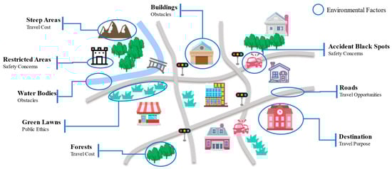
Figure 2.
The environmental factors of human mobility.
Currently, numerous trajectory forecasting methods have been developed and applied in various fields, such as autonomous driving [16], traffic management [17], and intelligent robotics [18]. Existing trajectory forecasting methods can be generally categorized into three types: traditional methods, machine learning methods, and deep learning methods. Traditional methods model the movement process of moving objects through physical or mathematical formulas, thereby achieving future trajectory forecasting. Such methods are characterized by their reliance on prior knowledge while typically offering the advantages of simplicity and efficiency. Representatives include the Kalman filtering method [19,20], Hidden Markov Models (HMMs) [21], particle filtering algorithms [22], etc. Machine learning methods achieve trajectory forecasting through efficient data-driven learning. Such methods implicitly learn the movement trends of the moving objects from large amounts of historical trajectory data, acquiring the capacity to handle more complex nonlinear relationships. Representatives include the Random Forest method [23], the Gradient Boosting Decision Tree method [24], and the K-Nearest Neighbors method [25]. The deep learning method is a vital branch of the machine learning method. Such methods can perform deep and nonlinear feature extraction on historical trajectory states and thereby forecast future trajectory states through mapping functions. With their strong capability in automatic feature learning, deep learning methods can achieve high-precision forecasting performance. Meanwhile, data intensiveness is also a major characteristic of deep learning methods. Representatives include Long Short-Term Memory (LSTM) [26], Gated Recurrent Unit (GRU) [27,28], and Seq2Seq [29]. However, existing methods face several limitations when applied to the forecasting scenario of human mobility that arises from daily urban activities. Most of the existing approaches fail to simultaneously consider the prior knowledge of human movement patterns and the heterogeneous effects of environmental factors. Thereby, they lack the ability to accurately and robustly forecast human mobility trajectories in the complex urban environment [30].
In our study, we formulate human mobility actions in daily urban activities as reactions to specific environmental factors. Consequently, we developed an environment-driven trajectory forecasting method that adapts to complex forecasting needs. Specifically, we begin by classifying different movement patterns; notable examples include convergence, divergence, and leadership. Since the influence of the geographical environments on human mobility varies depending on the prior patterns, we established several indicator systems for each movement pattern based on prior knowledge to quantify these heterogeneous effects. During the forecasting process, these indicator systems are utilized to generate potential fields, representing the calibrated probability of the next-step mobility direction. A gradient descent algorithm is then employed on these potential fields to determine the next-step mobility location. By treating the forecasted location as the current state of the trajectory, the method can support robust long-term forecasting. Furthermore, since there are no parameters in this environment-driven method that need to be trained, efficient real-time forecasting is also feasible.
The contributions of this study can be summarized as follows:
- (1)
- Human mobility in daily urban activities is significantly influenced by geographical environments. Hence, we developed an environment-driven trajectory forecasting method. Specifically, a potential field model and a gradient descent algorithm to simulate the heterogeneous effects of geographical environments during the forecasting process.
- (2)
- In order to incorporate the prior knowledge about different movement patterns, the indicator system is tailored to each type of movement pattern, which systematically summarizes the types of environmental factors that impact human mobility and their specific effects.
- (3)
- The effectiveness of the proposed method is validated on the synthetic trajectory dataset containing multiple movement patterns. Experimental results demonstrate that compared to data-driven approaches, the proposed method can achieve a stable forecasting performance under different environmental conditions and movement patterns.
The remainder of this paper is organized as follows. Section 2 provides a review of related work in the field of human mobility trajectory forecasting. Section 3 outlines the study area and the datasets used in this study. Section 4 provides a detailed description of the proposed human mobility trajectory forecasting method. Section 5 presents and discusses the experimental results. Finally, Section 6 concludes the paper and suggests future research directions.
2. Related Works
Trajectory forecasting, particularly in the context of human mobility arising from daily urban activities, has been widely researched across various domains. Existing forecasting methods can be generally divided into three major categories: traditional methods, machine learning methods, and deep learning methods. Each of these methods has its strengths and weaknesses, particularly in terms of robust long-term and real-time dynamic forecasting.
2.1. Traditional Methods
Traditional methods for human trajectory forecasting primarily rely on statistical models and mathematical techniques that utilize historical data. These models often focus on creating deterministic or probabilistic frameworks to forecast human mobility.
One of the earliest and most prominent methods for human mobility trajectory forecasting is the Kalman Filter method, which is widely used in linear dynamic systems [31,32]. For instance, Motai et al. [20] proposed a novel trajectory forecasting method that combines Kalman filtering and optical flow, enabling reliable real-time trajectory forecasting in dynamic environments. Additionally, Markov Chains and HMMs have also been employed to forecast trajectories based on previous states [20,33]. Qiao et al. [34] developed a hybrid Markov-based model for predicting non-Gaussian mobility data, achieving over 56% accuracy by adapting to individual mobility patterns and spatio-temporal characteristics. Furthermore, Lv et al. [35] utilized HMMs to enhance spatio-temporal mobility forecasting, demonstrating that incorporating individuals’ living habits improves mobility forecasting accuracy across diverse groups. Another notable advancement was introduced by Fox et al. [22], who applied particle filters as an improvement over Kalman filters, particularly beneficial for real-time applications like robot localization. This method proved effective in handling nonlinear, non-Gaussian noise, making it suitable for dynamic daily activities, such as real-time obstacle monitoring.
While traditional methods excel in real-time forecasting with linear and structured environments, they often falter when dealing with complex and highly variable environments. Their lack of adaptability hinders their ability to account for intricate movement patterns and long-term trends in human mobility.
2.2. Machine Learning Methods
With the rise in computational power, machine learning techniques have gained prominence in trajectory forecasting for human mobility. These methods are capable of handling more complex data but typically require large datasets for accurate forecasting.
Papathanasopoulou et al. [23] employed Random Forest algorithms to classify human movement based on factors such as gender, walking pace, and distraction, achieving high accuracy. However, their study was limited by the use of experimental data from a controlled environment, which may not fully capture the variability of real-world pedestrian movements. Similarly, He et al. [24] applied Gradient Boosting Decision Trees to predict human mobility patterns, demonstrating the model’s capability to capture complex, nonlinear relationships between environmental factors and human movement, though they faced challenges with dataset sparsity and missing values, which may impact prediction accuracy. Additionally, Yu et al. [25] employed K-Nearest Neighbors (KNN) for short-term traffic condition predictions, achieving effective results by incorporating spatial and temporal parameters. While the model demonstrated good accuracy, it struggled with long-term predictions. Cho et al. [36] investigated the influence of social ties on human mobility forecasting, revealing significant impacts of social connections on movement patterns, thus enhancing forecasting accuracy. Moreover, Song et al. [11] examined the predictability of human mobility using large-scale location-based data, concluding that individual mobility is highly predictable, which has significant implications for forecasting models.
While machine learning methods provide greater flexibility and are able to capture nonlinear relationships, they often require extensive training data and can be computationally intensive, which limits their real-time applicability.
2.3. Deep Learning Methods
The advent of deep learning has revolutionized trajectory forecasting. Deep neural networks are capable of modeling complex movement patterns in human daily activities. However, these models come with challenges, particularly when real-time predictions are required.
Alahi et al. [26] proposed a Long Short-Term Memory (LSTM)-based model to predict human trajectories in crowded environments, where the LSTM excels in learning long-term dependencies, making it ideal for sequential data, such as trajectory prediction. Graph Convolutional Networks (GCNs) have also been effectively utilized in pedestrian trajectory prediction by modeling complex interactions and long-term tendencies, with innovations like Sparse GCN (SGCN) [27] and attention-based GCN (AVGCN) [28] further enhancing accuracy in dynamic environments. Karatzoglou et al. [29] introduced Seq2Seq models for long-term human mobility forecasting, effectively translating input sequences into output sequences for more accurate forecasting in continuous time-series data. Vemula et al. [37] implemented attention-based models for trajectory prediction, allowing the model to focus on the most relevant parts of the data. This approach enhanced both the accuracy and interpretability of forecasting. Further advancements include the work by Jia et al. [38], where they proposed an Attention-LSTM model for aircraft trajectory forecasting, demonstrating higher forecasting accuracy by focusing on influential factors. In another study, Lin et al. [39] explored the use of LSTMs with spatial-temporal attention mechanisms for trajectory forecasting, highlighting the model’s ability to explain the influence of historical trajectories and surrounding environments. Additionally, research by Lv et al. [40] and Peng et al. [41] has shown promising results in the application of LSTM and attention mechanisms for trajectory forecasting, respectively.
Deep learning methods offer unparalleled accuracy in capturing complex movement patterns and making long-term forecasts [42,43]. However, the computational demands of these models, combined with the large datasets required for training, often hinder real-time applicability [44].
In summary, traditional methods provide effective real-time trajectory forecasting but have limitations in handling complex movement patterns with robustness over long-term periods. Machine learning methods present greater flexibility but usually at the cost of computational efficiency. Deep learning techniques deliver high accuracy, particularly for long-term forecasting, but also struggle with maintaining computational efficiency. Therefore, our study aims to fill these gaps by integrating potential field theory with movement patterns, improving forecasting performance in terms of both efficiency and robustness. The potential field method, which simulates the heterogeneous effects of geographical environments, ensures computational feasibility for dynamic real-time applications, while incorporating pattern-based knowledge enhances long-term forecasting accuracy, minimizing the compounding errors typical of data-driven approaches.
3. Study Area and Data Description
3.1. Study Area
The study area is the Zhongzheng District of Taipei, an urban region known for its dense population. The area’s urban landscape features a mix of natural, economic, and cultural areas, making it ideal for studying trajectories of human mobility arising from daily urban activities. As shown in Figure 3, the area’s diverse features, including roads, buildings, and water bodies, create an environment for examining how geographical environments affect human mobility trajectories.
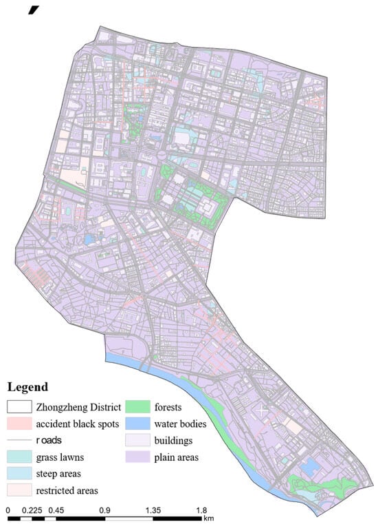
Figure 3.
Overall study area with distributions of different environmental factors.
3.2. Synthetic Trajectory Dataset
We used a synthetic trajectory dataset to evaluate forecasting performance via a hybrid simulation framework. This framework is driven by prior knowledge and practical data to generate a reliable and adaptive dataset. Specifically, the prior knowledge is utilized to define basic simulation rules for each type of movement pattern. And the practical dataset, GeoLife [45,46,47], is utilized to provide reference information, improving the simulation reliability within our target study area. To ensure the applicability of the GeoLife dataset to our target study area, we carefully considered the similarities between Beijing (the primary location of GeoLife trajectories) and Taipei. Both cities are highly urbanized, and economically developed, and exhibit similar industrial structures and urban mobility patterns. These shared characteristics support the transferability of human mobility knowledge derived from the GeoLife dataset to our target study area, thereby enhancing the reliability of the synthetic trajectory dataset in representing realistic movement scenarios [48,49,50].
The prior knowledge of different movement patterns is summarized as follows: First, the convergence pattern is typically destination-oriented. It requires the fastest arrival to the destination, which is generally an important public place. Second, for the divergence pattern, on the contrary, its starting location is generally a public place. And without an urgent need for arrival, it would first pass through certain waypoints for other activities before ultimately reaching the destination. Third, the leadership pattern is typically leader mobility-oriented. It primarily focuses on the movement speed of the leader and the queue of the followers. Therefore, we clarify the key points for different movement patterns’ simulation, which is briefly presented in Table 1. The specific simulation rules for each pattern are introduced in the following sections.

Table 1.
Key points for different movement patterns’ simulation based on prior knowledge.
- (1)
- Trajectory simulation for the convergence pattern
To simulate the convergence pattern, we first extract reference information from the GeoLife dataset, including the alternative types of starting location and destination location (Algorithm 1). Then, based on the reference information and POI dataset, the starting location and destination location are randomly selected for a trajectory sample (Algorithm 2, lines 3–9). Third, the A* method is used to generate the shortest path from the starting location to the destination location (Algorithm 2, line 11). Finally, with the sparsification and randomization on the path (Algorithm 2, lines 13–18), the trajectory sample can be generated.
| Algorithm 1: Reference information extraction from the GeoLife dataset for the convergence pattern |
| Input: GeoLife trajectory dataset ; POI dataset in Beijing minimum frequency threshold |
Output: alternative set for the selection of starting and destination location types
|
| Algorithm 2: Trajectory sample simulation for the convergence pattern |
| Input: alternative set for the selection of starting and destination location types ; POI dataset in Taipei ; minimum distance threshold road network ; sampling frequency ; gauss noise parameters |
Output: simulated trajectory sample
|
- (2)
- Trajectory simulation for the divergence pattern
To simulate the divergence pattern, we first extract reference information from the GeoLife dataset, including the alternative types of starting location, waypoints, and destination location (Algorithm 3). It is worth noting that waypoint detection considers both movement attributes and semantic information (Algorithm 3, lines 9–12). Then, based on the reference information and POI dataset, starting location waypoints and destination locations are randomly sampled. Third, we generate a path using the A* method according to the order of these sampling points. And the trajectory sample is finally generated with a sparsification and randomization operation (these steps are similar to those in Algorithm 2).
| Algorithm 3: Reference information for the divergence pattern |
| Input: GeoLife trajectory dataset ; POI dataset in Beijing ; time threshold and distance threshold for stay-point detection algorithm ; minimum frequency threshold |
Output: alternative set for the selection of starting location, waypoints and destination location types
|
- (3)
- Trajectory simulation for the leadership pattern
To simulate the leadership pattern, we first extract reference information from the GeoLife dataset, including the alternative selections of movement speeds (Algorithm 4). Then, the leader trajectory is first generated (Algorithm 5, lines 4–18). The generation steps are similar to those previously described, with one major difference in the sparsification operation. Specifically, when sampling trajectory points along the path, the reference movement speeds should be taken into account (Algorithm 5, lines 13–14). Subsequently, the final follower trajectory is generated considering the following queue parameters (Algorithm 5, lines 20–22).
| Algorithm 4: Reference information for the leadership pattern |
| Input: GeoLife trajectory dataset |
Output: alternative set for the selection of movement speeds in trajectory
|
| Algorithm 5: Trajectory sample simulation for the leadership pattern |
| Input: alternative set for the selection of movement speeds in trajectory ; POI dataset in Taipei ; minimum distance threshold road network ; gauss noise parameters ; lag distance and offset angle for the followers’ queue |
Output: simulated trajectory sample
|
Finally, according to the defined simulation rules, we generated 100 trajectory samples for each type of movement pattern. Therefore, a synthetic trajectory dataset with diverse movement patterns and an abundant number of samples can be constructed for the subsequent experiments.
3.3. Environment Datasets
In our study, the environmental factors include nine categories, namely plain areas, roads, steep areas, forests, grass lawns, water bodies, buildings, restricted areas, and accident black spots. The environmental factors are acquired from multi-source geographical data. A detailed description of each category of environmental factors is presented in Table 2. And the spatial distribution of environmental data is visualized in Figure 4.
Table 2.
Description of environmental datasets.

Figure 4.
The spatial distribution of environmental data in this study. (a) Plain areas; (b) roads; (c) steep areas; (d) forests; (e) grass lawns; (f) water bodies; (g) buildings; (h) restricted areas; (i) accident black spots.
4. Methodology
4.1. Overall Framework
In our study, we propose an environment-driven trajectory forecasting method for human mobility arising from daily urban activities. In all, we formulate human mobility actions in daily urban activities as reactions to specific environmental factors. Firstly, as illustrated in Figure 5, considering the influence of the geographical environments on human mobility varies depending on the prior patterns, we develop different indicator systems for the convergence, divergence, and leadership patterns. These indicator systems comprehensively summarize the heterogeneous effects of environmental factors. Under the guidance of the indicator system of the corresponding movement pattern, the potential field is first generated to quantify the comprehensive effect of all environmental factors. Specifically, the potential field modeling includes two aspects. On the one hand, attractive and repulsive potential functions are constructed, respectively, to simulate the attraction or repulsion effect of environmental factors on human mobility. On the other hand, the weights of different environmental factors are determined in a hybrid manner. Thereby, a comprehensive potential field can be generated through the weighted sum manner, representing the calibrated probability of the next-step mobility direction. Finally, a gradient descent algorithm is then employed on the potential field to determine the next-step mobility location.
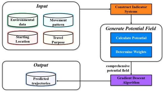
Figure 5.
Flowchart of the environment-driven trajectory forecasting method.
4.2. Indicator System Construction
The indicator system is developed to systematically identify what types of environmental factors are influencing human mobility and what specific effects they have. Specifically, the indicator system is structured into three levels.
The first level of the indicator system reflects the attractive or repulsive effect of environmental factors. Attractive factors, such as accessible roads and destinations, have a positive effect on human mobility. People are drawn to these factors for convenience or safety during the travel process. In contrast, repulsive factors, such as restricted areas, water bodies and obstacles, negatively influence the decisions of human mobility, pushing them toward alternative routes. Attraction and repulsion are the most fundamental manifestations of the heterogeneous effects of environmental factors.
The second level of the indicator system further refines the specific aspects of how attractive and repulsive factors affect human mobility. Attractive factors can be further refined into travel opportunities and travel purposes. Their detailed meanings are presented as follows:
- Travel Opportunities: Refers to the availability of paths or plain areas that facilitate easy movement through the urban spaces. Roads and open spaces offer flexibility and convenience in route selection, influencing decision-making and efficiency.
- Travel Purpose: Encompasses the motivations behind the movement, influencing trajectories in various ways. It can lead to convergence when individuals aim for a common destination, divergence when they disperse from a central point or a starting location, and leadership patterns when others follow a leader’s path. It helps shape movement patterns in daily activities and social contexts, reflecting both individual goals and group behavior.
Repulsive factors can be further refined into travel cost, public ethics, obstacles, and safety concerns. Their detailed meanings are presented as follows:
- Travel Cost: Represents the effort required to traverse specific terrains, such as steep inclines or forested areas. High travel costs are associated with challenging terrains that impede movement, making these areas less likely to be chosen for travel.
- Public Ethics: Social norms, such as avoiding walking on grass lawns, influence pedestrian trajectories. Ethical considerations and public rules can create restrictions on movement, even if these paths offer shortcuts.
- Obstacles: Physical barriers like water bodies or buildings prompt people to adjust their routes, avoiding direct paths to prevent collisions with these obstacles. These obstacles require detours but do not necessarily alter the overall trend of travel, simply influencing the specific paths taken.
- Safety Concerns: Relates to the perceived risk associated with certain areas, such as restricted areas or accident black spots. People are more likely to avoid unsafe routes, opting for paths that offer better security and lower risks [51].
The first and second levels of the indicator system provide a comprehensive understanding of the heterogeneous effect of environmental factors on human mobility. Then, the third level of the indicator system presents the specific environmental factors corresponding to the aforementioned classification.
The indicator systems for convergence, divergence, and leadership patterns differ in their focus on movement patterns and interactions with the environment. For the convergence pattern, factors attract people to a common point (destination), while restricted areas or obstacles act as repulsive forces. In divergence, the indicators emphasize dispersal opportunities and multiple path choices. For leadership patterns, the system focuses on how people follow a leader, with the leader’s influence being more important than other environmental factors. Each system reflects how people interact with their surrounding environments in different movement patterns. The indicator system constructed for the convergence pattern is shown in Figure 6. For divergence and leadership, the primary differences lie in two aspects: the travel purpose and the weight of environmental factors. Specifically, in convergence, the travel purpose is a shared destination; in divergence, it is the start location; and in leadership, it revolves around the leader’s trajectory. Additionally, the weights assigned to environmental factors vary across these patterns to reflect their unique influences on each pattern. The detailed calculation manner for these weights is provided in Section 4.3.3.
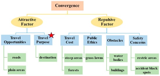
Figure 6.
The indicator system constructed for the convergence pattern. The red star is used to indicate that “Travel Purpose” is the most significant factor among them.
4.3. Potential Field Modeling
4.3.1. Overview for Modeling Approach
Potential field modeling is employed to comprehensively and quantitatively simulate the effect of environmental factors on human mobility [52,53]. The potential field method conceptualizes the environment as a field of forces, where environmental factors typically exert two types of forces, i.e., attractive or repulsive forces, on human mobility. The combined effects of these two types of forces finally determine the trajectories on which people are likely to travel [54].
Based on the abovementioned indicator system constructed in a top-down manner, we can now calculate the potential field, which comprehensively forms the effect of all environmental factors on human mobility from a bottom-up perspective. Specifically, the potential at a location is computed as a weighted sum of the potentials from each type of environmental factor,
where is the total potential at the location . is the total number of environmental factors. is the weight associated with the -th factor, reflecting its relative importance. is the potential contribution from the -th environmental factor. It can be divided into two categories, i.e., attractive potential and repulsive potential . They use a different computation manner. The next two subsections would describe in detail how to construct the two types of potential functions and how to determine the weights of the environmental factors.
4.3.2. Attractive and Repulsive Potential Functions
Considering the attractive force can pull the people towards the attractive factors, the attractive potential can be typically calculated by the following potential function:
where is the attractive potential at location . is the attraction gain coefficient. represents the location of the attractive factors closest to the location . represents the distance between location and its closest attractive factors. is the trigger threshold. is the influence range of the attractive factors. Once the people get into the effect range of attractive factors, the attractive potential would significantly decrease as the distance between the people and the attractive factors gets smaller. It can ensure that the people are increasingly attracted as they get closer to the attractive factors.
On the contrary, the repulsive force is designed to push the people away from the repulsive factors. The repulsive potential can be typically calculated by the following potential function:
where is the repulsive potential at location . is the repulsion gain coefficient. represents the location of the repulsive factors closest to the location . represents the distance between location and its closest repulsive factors. is the trigger threshold, and is the influence range of the repulsive factors. This repulsive potential would significantly increase as the people get closer to a repulsive factor, thus exerting a repulsive force that pushes the people away from potential collisions.
The meanings and setting values of the hyperparameters in Formulas (2) and (3) are further explained in this paragraph. Taking the convergence pattern as an example, the distances calculated in Equations (2) and (3) are based on the shortest distance from the nearest line or polygon geometry. Notably, there is a small threshold value where distances within this range are assigned a value of to prevent the potential from becoming infinitely large, especially when the point is inside the polygon. Conversely, represents the influence range; beyond this range, the potential is set to zero. The gain coefficients (/) and influence radius () for each factor are set as constants for all environmental factors to simplify the model’s complexity and enhance its generalization capabilities. Constant hyperparameters are commonly used in spatial interaction and potential field models, such as the gravitational coefficient in human mobility studies, to represent stable relationships between human and environmental factors [55,56]. Similarly, the fixed influence radius helps clearly define the spatial scope of environmental factors’ effects, similar to the service radius concept in urban facilities planning [57]. Except for the travel purpose, it has a global influence and is not restrained by a finite radius.
4.3.3. Manner for Determining the Weights of Environmental Factors
In addition, the other important elements in Equation (1), namely the weights for different types of environmental factors, are required to be determined. Each environmental factor’s potential field is represented as a 2D potential field array. The weights are used to aggregate these arrays into a composite potential field for subsequent trajectory forecasting. In our study, the weights for different types of environmental factors are determined by a combined weighting manner. Specifically, this manner integrates both the subjective expert scoring method and the objective entropy weight method. For each type of movement pattern, the details of the weighting manner are described as follows.
- (1)
- Subjective expert scoring method
The expert scoring method incorporates domain knowledge to determine weights [58]. A structured questionnaire was distributed to 20 domain experts, who evaluated the factors across five levels of importance: Highly Important (Score 5), Moderately Important (Score 4), Neutral (Score 3), Slightly Important (Score 2), and Not Important (Score 1). The detailed results of the expert scoring survey are shown in Appendix A. It is worth noting that the expert scoring survey results are, respectively, obtained for the convergence, divergence, and leadership patterns. For the -th environmental factors, its total score evaluated by an expert is calculated by
where represents the total score of the -th environmental factors. represents the number of importance levels. represents the number of -th importance levels received from experts for the -th environmental factor. represents the basic score of the -th importance level. Then, the weight for the -th environmental factor is calculated by the proportion of its score in the total score, using the following equation:
where represents the weight for the -th environmental factor determined by the subjective expert scoring method.
- (2)
- Objective entropy weight method
The entropy weight method is a data-driven method that objectively reflects the importance of environmental factors based on their variability across data samples [59]. The detailed calculation steps are as follows. Firstly, it needs to perform the data normalization operation. The raw data of each environmental factor is normalized to ensure comparability,
where represents the normalized potential value, and and are the minimum and maximum potential values for the -th environmental factor, respectively. Then, it needs to calculate the information entropy. The entropy for the -th environmental factor is computed as follows:
where represents the proportion of the sample in location for the -th environmental factor. and represent the numbers of locations in width and height, respectively.
Finally, it needs to determine the objective weight based on information entropy. For a certain environmental factor, the smaller its information entropy value, the greater the dispersion degree it has, and the more important information it reflects. Therefore, it requires a larger weight. Then, the objective weight for the -th environmental factor is calculated as follows:
- (3)
- Weight combination
The final weight for each factor is a linear combination of objective and subjective weights and is as follows:
where represents the proportion of reliance on entropy weighting, set at 0.5 in this study based on empirical validation. The weights are applied in the potential field model to scale the influence of each environmental factor’s potential field when summing their contributions. This ensures that both data-driven insights and expert judgment are reflected in the trajectory forecasting. This combined approach balances objectivity and domain relevance, enhancing model robustness and interpretability. The calculated results of the combined weights are also presented in Appendix A.
4.4. Gradient Descent Algorithm for Trajectory Forecasting
Based on the modeling result of the potential field, the gradient descent algorithm is utilized to implement the trajectory forecasting process. In the potential field, as illustrated in the pseudo-code of Algorithm 6, people travel from a starting location. During the travel process, people tend to move towards locations with low potential while simultaneously avoiding locations with high potential until they ultimately reach the destination location. To achieve the optimal trajectory forecasting, the gradient descent algorithm can be applied. First, in the initialization step, the location is set to , the iteration index is initialized to 0, and then is added to the trajectory sequence (Algorithm 6, lines 1–2). In the while loop, the next location is calculated at each step by subtracting from and is added to the trajectory sequence (Algorithm 6, lines 4–5). Here, the direction of the gradient indicates the direction in which the potential changes fastest. The learning rate is determined based on the walking speed of pedestrians in the simulation. It controls the step size of each iteration, ensuring that the movement is neither too fast nor too slow [60]. The loop runs until the Euclidean distance between and is less than a step size or exceeds maximum iterations (Algorithm 6, line 3). An example of the trajectory forecasting using the gradient descent algorithm is also visualized in Figure 7.
| Algorithm 6: Gradient descent algorithm for trajectory forecasting |
| Input: starting location , destination location , potential filed which simulates environment effects, learning rate , step size , maximum iterations |
Output: forecasted trajectory
|
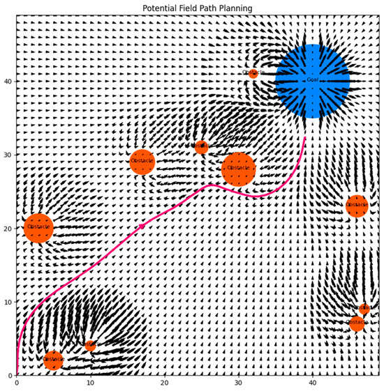
Figure 7.
Illustrates a forecasted trajectory using the gradient descent algorithm in the potential field. The trajectory of human mobility is influenced by the attractive force and repulsive forces of the environmental factors. The black arrow represents the gradient direction of the potential function at each location.
5. Experiments and Discussions
5.1. Evaluation Metrics
The forecasting performance of the proposed method is evaluated using the following three metrics:
- (1)
- Average Displacement Error (ADE) [61]: ADE measures the mean squared distance between the forecasted location and the actual location. It is calculated as follows:where is the actual location at time for the -th target, is the forecasted location, is the number of targets, and is the number of forecasting time steps.
- (2)
- Maximum Absolute Error (MaxAE) [62]: MaxAE is the maximum observed distance between the forecasted and actual trajectory. It is calculated as:where is the actual location at time for the -th target, is the forecasted location.
- (3)
- Miss Rate (MR) [63]: MR is the proportion of trajectories where the forecasted location exceeds a threshold distance from the actual position, as illustrated in Figure 8. The formula is as follows:where is the total number of trajectories, and is the number of missed forecasted locations (those exceeding the threshold).
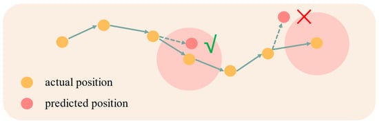 Figure 8. Process of calculating MR.
These metrics help in assessing the overall accuracy (ADE), worst-case performance (MaxAE), and model failures (MR).
5.2. Comparisons with Baseline Methods
To assess the effectiveness of the potential field approach, a comparison was made with Kalman Filter and LSTM baselines using metrics including ADE, MaxAE, and MR, as presented in Figure 9. Multi-step prediction involves forecasting several future time steps based on previous observations and predictions, allowing for a comprehensive evaluation of each model’s performance over extended horizons. The results indicate that the potential field model generally outperforms the other two methods in long-term predictions.

Figure 9.
The comparison of experimental results with baseline methods, including Kalman Filter and LSTM, uses three metrics: (a) ADE; (b) MaxAE; (c) MR.
As also shown in the examples in Figure 10, one of the key advantages of the potential field approach is its ability to maintain low ADE and MaxAE across multiple forecasting steps. This demonstrates its robustness and reliability in accurately forecasting human mobility trajectories, even when the forecasting time step extends or when situations such as turns are encountered. Although the potential field model may not outperform LSTM in short-term forecasting (one, three, or five steps), it excels in longer-term forecasting (ten steps), showcasing its stability and long-term advantages. Furthermore, the potential field model exhibits a lower MR, indicating that it effectively minimizes the occurrence of significant forecasting errors.
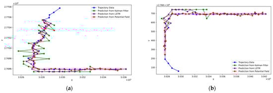
Figure 10.
The comparison of predicted trajectories of different models on the dataset. (a) shows the overall trend of the predicted trajectories of different models in a continuous time—series. It can be clearly observed that our potential field model maintains stable predictions over a relatively long period, with less deviation and more consistent trends compared to the other two models. (b) a scenario with significant turns in the trajectory is presented. Here, it is evident that our potential field model can also handle turns better than Kalman Filter and LSTM.
In contrast, the Kalman filter, despite being widely used in various prediction applications, exhibits notably higher values for ADE, MaxAE, and MR across all three metrics. These errors increase significantly as the prediction step increases. The primary reason for this performance drop might be explained from two aspects. On the one hand, Kalman filters are designed for systems with linear dynamics and Gaussian noise, making them less effective in real-world urban environments where the environment is complex and highly nonlinear. On the other hand, the Kalman filter does not account for the underlying movement patterns, such as convergence, divergence, or trendsetter behaviors. This absence of consideration for human movement patterns and complex environmental factors means that the Kalman filter is unable to capture the full range of influences that drive mobility, which is essential for accurate trajectory forecasting in urban environments. Furthermore, the potential field model incorporates both complex environmental factors and prior movement patterns, which contributes to its superior performance in long-term forecasting. Although LSTM models are capable of learning from historical data and performing well in short-term predictions, they also struggle to maintain accuracy over longer prediction steps, primarily due to error accumulation.
Overall, the potential field method stands out for its ability to provide stable and accurate trajectory forecasting, making it particularly suitable for daily urban activities where understanding human mobility is critical for traffic management and safety. This trend highlights the model’s potential as a preferred choice for urban trajectory forecasting.
5.3. Forecasting Accuracy Results Under Different Movement Patterns
Based on the experimental results from Table 3, which compares the forecasting performance of the model based on potential fields under different movement patterns, slight variations are observed. For the ADE, the convergence pattern shows an average trajectory error of 9.96, which is slightly higher than the divergence (6.22) and leadership patterns (8.24). However, the MR and MaxAE show no significant differences across the patterns, indicating that the prediction algorithm maintains strong stability and robustness across different movement patterns.
Table 3.
The comparison of experimental results under different movement patterns: convergence, divergence, and leadership.
Upon further analysis, the MR for all patterns remains within the range of 9.30% to 11.25%, showing that the forecasting algorithm adapts well to different movement patterns and maintains a low error rate in most cases, which is crucial for real-world applications. In terms of MaxAE, all movement patterns recorded the same error of 141.42. While the divergence pattern is characterized by its inherent uncertainty and exploratory nature, which might suggest variability, the consistent MaxAE across all three modes indicates that the prediction model effectively handles the complexities of each movement pattern. This uniformity reinforces the model’s robustness and reliability in trajectory forecasting, demonstrating that it can maintain performance despite the distinct behaviors associated with convergence, divergence, and leadership patterns.
In conclusion, the prediction model based on potential fields demonstrates strong prediction accuracy and stability across various movement patterns, making it an effective method for trajectory forecasting.
5.4. Capability Analysis of Real-Time Forecasting
The potential field approach has demonstrated remarkable efficacy in real-time trajectory forecasting applications. In contrast to deep learning models that often grapple with latency due to their intensive computational requirements, the potential field method offers expedited predictions, achieving a response time of less than 1 s per update. This swift response capability is crucial for real-time systems, as it allows for dynamic adjustment of forecasting based on the latest environmental data. In this study, with historical data as a reference, the method is capable of providing long-term trajectory forecasting for more than 30 min based on positional sampling intervals of 3 min. Moreover, the average accuracy of these forecasting processes is maintained at no less than 85%. This level of accuracy underscores the method’s reliability and effectiveness in long-term trajectory forecasting, which is particularly valuable for applications requiring precise and sustained predictive insights. This level of performance is highly beneficial for applications that require precise and timely trajectory guidance over extended periods. As depicted in Figure 11, the potential field method’s efficiency is evident, making it an ideal choice for systems that demand both dynamic real-time and robust long-term forecasting capabilities.
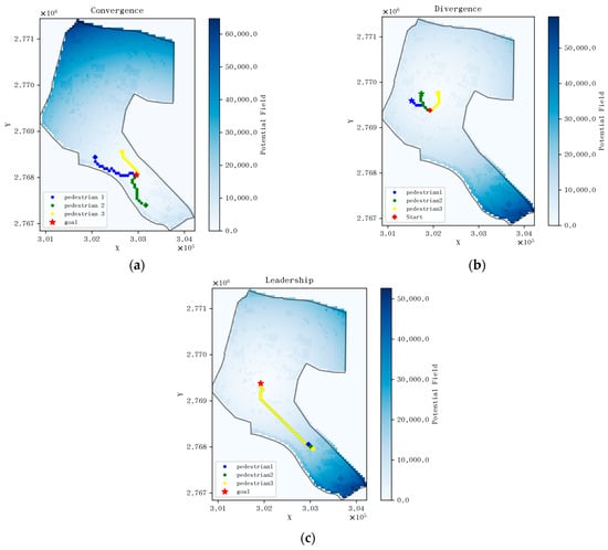
Figure 11.
(a) Visualizes the trajectory forecasting result for the convergence pattern; (b) visualizes the trajectory forecasting result for the divergence pattern; (c) visualizes the trajectory forecasting result for the leadership pattern.
5.5. Evaluation of Data Sensitivity
This section presents an analysis of the model’s performance under varying conditions of data availability in a fifteen-step prediction. With results summarized in Table 4, by comparing the model’s accuracy with complete environmental data against the conditions lacking specific environmental data categories, we assess the impact of each indicator on trajectory forecasting.
Table 4.
The comparison of experimental results under different missing conditions of environmental data.
The results show that the model maintains robust forecasting accuracy even when some environmental data are unavailable. The absence of “Travel Opportunities” and “Travel Cost” data results in slight increases in ADE to 28.34 and MaxAE to 1364.73, with minimal changes in MR. Similarly, the lack of “Public Ethics” data shows a comparably smaller impact, with ADE increasing to 28.10, indicating that these factors, while influential, do not critically impair the model’s performance. However, the absence of “Obstacles” data significantly affects forecasting accuracy, with ADE rising to 29.08, MaxAE to 1400.00, and MR increasing to 12.20%. These results underline the critical role of obstacle-related data, such as water bodies and buildings, in shaping pedestrian trajectories. Furthermore, missing “Safety Concerns” data also leads to a notable degradation in performance, with ADE increasing to 29.21 and MR to 12.05%, reflecting the importance of accurately accounting for safety-related factors in trajectory forecasting.
Furthermore, we compare the results of the experiments with combined missing data, as shown in Figure 12. Both rows and columns represent the missing data categories. Hence, the results are symmetric matrices and the values on the diagonal correspond to the cases where only a single category of data is missing. The results of combined missing data further validate the conclusion drawn from the cases of single-category missing data. When data on “Travel Opportunities”, “Travel Cost”, and “Public Ethics” are missing in pairwise combinations, the three metrics (ADE, MaxAE, and MR) are generally smaller. This indicates that the absence of these data combinations has a relatively smaller impact on the results. Conversely, when data on “Obstacles” and “Safety Concerns” are missing in combination, the three metrics are generally larger. This significant increase in the metrics suggests that the lack of information regarding obstacles and safety has a substantial negative impact on the model’s performance, highlighting the crucial role these two factors play in accurately predicting the trajectories.
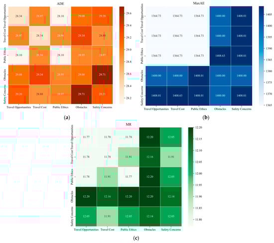
Figure 12.
The comparison of experimental results under combined missing conditions of environmental data. The values on the diagonal are the results of experiments with single missing data. (a) ADE; (b) MaxAE; (c) MR.
In summary, while the model demonstrates resilience in the face of environmental data absence, the type of missing data significantly influences its forecasting performance. The experiments underscore the necessity of incorporating diverse environmental factors for improved accuracy and reliability in trajectory forecasting. Future research will investigate methods for mitigating data sensitivity, such as data imputation techniques or integrating complementary data sources to further enhance model robustness under variable data conditions.
6. Summary and Outlook
6.1. Conclusions
This paper presents a novel environment-driven trajectory forecasting method that leverages potential field theory to model human mobility in urban environments. The methodology integrates the prior knowledge of movement patterns and the heterogeneous effects of geographical environments to provide robust and adaptive trajectory predictions for daily urban activities. The main contributions of the study are summarized as follows:
- (1)
- The study introduces a unique approach to incorporate prior movement patterns, including convergence, divergence, and leadership, into the trajectory forecasting process. This integration allows the model to account for distinct mobility behaviors, enhancing its applicability across various scenarios.
- (2)
- By systematically constructing indicator systems for environmental factors, the method quantifies the effects of heterogeneous geographical environments on human mobility. The combination of attractive and repulsive potential fields provides a robust framework for modeling complex environmental effects.
- (3)
- The proposed method employs a hybrid weighting approach, combining expert scoring and entropy weight methods to assign weights to environmental factors. This ensures both data-driven objectivity and domain-specific relevance, resulting in a calibrated potential field that reflects real-world dynamics.
- (4)
- The proposed methodology is extensively evaluated on synthetic trajectory datasets representing various movement patterns. It demonstrates superior performance in long-term forecasting compared to Kalman filter and LSTM models, showcasing its robustness and reliability.
6.2. Implications for Practice
The practical future implications of this study are substantial, particularly in aspects such as effective traffic management, dynamic resource allocation, and sustainable urban development.
In terms of effective traffic management, the model can be used to forecast human mobility paths in high-density areas, informing traffic signal timings and road designs. This capability allows city planners to anticipate pedestrian navigation at critical intersections, thereby reducing congestion and enhancing safety. However, as the complexity of the environment increases, computational demands may grow significantly due to the combinatorial nature of pedestrian interactions. To address this challenge, strategies such as modular zoning, which involves dividing large areas into smaller computational units, or integrating edge computing technologies, can help maintain real-time responsiveness in practical applications.
For resource allocation, the model facilitates the strategic placement of resources such as bike-sharing stations or pedestrian signage. By forecasting how people are likely to move through different spaces, city services can be dynamically distributed to optimize facility usage and minimize waste. However, when applied at a city scale, such as across multiple commercial or residential districts, computational bottlenecks may arise due to complex spatial topologies, including elevated walkways or multi-layer road systems. A prioritized approach that focuses on transient high-traffic zones, such as subway stations during rush hours, rather than attempting city-wide synchronization, can enhance computational efficiency while preserving the model’s utility.
In the context of sustainable urban development, the model aids in optimizing urban designs to promote walking and cycling and reduce vehicular congestion. By strategically positioning green corridors, bike lanes, and walking trails based on predicted pedestrian paths, more eco-friendly transportation options can be encouraged in cities. However, simulating extended time horizons, such as annual predictions, introduces dynamic variables like weather and events, which may strain computational resources. To mitigate this, incremental updates that refine model parameters iteratively using historical data, rather than performing full recomputations, offer a practical solution to reduce computational overhead in long-term scenarios.
Overall, the study underscores the critical role of human mobility trajectory prediction in achieving sustainable urban environments, supporting the shift towards more livable and eco-friendly cities. It underscores the importance of balancing precision and computational efficiency, particularly in large-scale or long-term applications. Faced with more complex environments, combinations with other lightweight algorithms can also be considered.
6.3. Research Deficiency
While the model demonstrated strong performance, it does have some limitations. First, the model relies heavily on the accuracy and completeness of environmental data, such as roads, buildings, and other geographical features. In practical applications, these data may be outdated, incomplete, or unavailable in real time, which could compromise the reliability of the model. Second, the current indicator system assumes static environmental conditions, which do not account for dynamic changes like temporary infrastructure modifications, weather conditions, or road closures. These changes can have a significant impact on human mobility patterns and are not yet fully addressed in the current framework. Finally, the evaluation of the model primarily relies on the synthetic trajectory dataset. Despite the representative advantages of synthetic datasets, they may not fully reflect the complexity and variability of real-world human mobility. The validation under large-scale real-world trajectory remains to be further realized.
6.4. Future Research
To address these limitations, future research will focus on the following directions:
- (1)
- The integration of dynamic environmental data, such as real-time traffic conditions, weather updates, or temporary road closures, will be explored. Incorporating these dynamic inputs into the potential field modeling process would allow the model to better adapt to rapidly changing urban environments, significantly improving its robustness and applicability in complex environments.
- (2)
- Recognizing the need for real-world validation, future efforts will include the collection of real-world trajectory data. This will involve conducting volunteer-based studies, where participants provide detailed travel purposes and mobility trajectories through surveys and GPS tracking. Additionally, collaborations with transportation agencies and urban planning organizations will be pursued to access comprehensive datasets, ensuring that the model is tested and validated in diverse and practical scenarios.
- (3)
- Future studies will also aim to integrate social and behavioral factors into the model. Factors such as group dynamics, individual preferences, and social interactions could provide a richer understanding of human mobility and lead to more accurate trajectory forecasting.
- (4)
- Exploring hybrid models that combine the advantages of deep learning for feature extraction and the potential field method for real-time decision-making is another promising direction. Such approaches could enhance both short-term accuracy and long-term stability in trajectory forecasting, particularly in highly dynamic urban environments.
Author Contributions
Conceptualization, K.C. and P.Z.; methodology, K.C. and P.Z.; software, P.Z.; validation, K.C., P.Z., J.L., M.D., Q.G., C.Y., J.C. and X.P.; formal analysis, P.Z.; investigation, P.Z.; resources, J.L., M.D., Q.G., C.Y., J.C. and X.P.; data curation, P.Z.; writing—original draft preparation, P.Z.; writing—review and editing, K.C.; visualization, P.Z.; supervision, J.L., M.D., Q.G., C.Y., J.C. and X.P.; project administration, J.L., M.D., Q.G., C.Y., J.C. and X.P.; funding acquisition, J.L., M.D., Q.G., C.Y., J.C. and X.P. All authors have read and agreed to the published version of the manuscript.
Funding
This research was funded by Key R&D Plan Projects in Hebei Province, grant number 22340301D, China Postdoctoral Science Foundation, grant number 2021M703021, and Hebei Postdoctoral Science Foundation, grant number B2021003031.
Institutional Review Board Statement
Not applicable.
Informed Consent Statement
Not applicable.
Data Availability Statement
The data presented in this study are available on request from the corresponding author due to privacy. The codes supporting the findings of this study are available at https://github.com/code-1949/Trajectory-Forecasting-via-Potential-Field, accessed on 15 January 2025.
Acknowledgments
We thank anonymous reviewers for their comments on improving this manuscript.
Conflicts of Interest
Authors Jingyi Liu, Qi Guo, Chen Yao, Jinyong Chen and Xinyu Pei were employed by The 54th Research Institute of China Electronics Technology Group Corporation. The remaining authors declare that the research was conducted in the absence of any commercial or financial relationships that could be construed as a potential conflict of interest.
Appendix A
The results of the expert scoring survey are summarized in Table A1, Table A2 and Table A3, which categorizes the environmental factors based on their perceived importance. The table lists the total number of responses for each level of importance—Highly Important (Score 5), Moderately Important (Score 4), Neutral (Score 3), Slightly Important (Score 2), and Not Important (Score 1). The aggregated scores reflect expert evaluations and form the basis for calculating subjective weights. This structured scoring method ensures that the relative significance of each factor aligns with domain expertise while complementing the objective entropy weighting process. The final calculated results of the combined weights are also presented in Table A4, Table A5 and Table A6.
Table A1.
The results of the expert scoring survey for the convergence pattern.
Table A1.
The results of the expert scoring survey for the convergence pattern.
| Data | Highly Important | Moderately Important | Neutral | Slightly Important | Not Important |
|---|---|---|---|---|---|
| Plain areas | 12 | 6 | 2 | 0 | 0 |
| Roads | 16 | 4 | 0 | 0 | 0 |
| Destination | 20 | 0 | 0 | 0 | 0 |
| Steep areas | 10 | 6 | 3 | 1 | 0 |
| Forests | 9 | 7 | 3 | 1 | 0 |
| Grass lawns | 6 | 5 | 6 | 3 | 0 |
| Water bodies | 12 | 5 | 2 | 1 | 0 |
| Buildings | 14 | 6 | 0 | 0 | 0 |
| Restricted areas | 18 | 2 | 0 | 0 | 0 |
| Accident black spots | 12 | 6 | 2 | 0 | 0 |
Table A2.
The results of the expert scoring survey for the divergence pattern.
Table A2.
The results of the expert scoring survey for the divergence pattern.
| Data | Highly Important | Moderately Important | Neutral | Slightly Important | Not Important |
|---|---|---|---|---|---|
| Plain areas | 13 | 5 | 2 | 0 | 0 |
| Roads | 15 | 5 | 0 | 0 | 0 |
| Start | 14 | 4 | 2 | 0 | 0 |
| Steep areas | 8 | 6 | 4 | 2 | 0 |
| Forests | 7 | 8 | 4 | 1 | 0 |
| Grass lawns | 5 | 6 | 6 | 3 | 0 |
| Water bodies | 10 | 5 | 4 | 1 | 0 |
| Buildings | 12 | 7 | 1 | 0 | 0 |
| Restricted areas | 16 | 4 | 0 | 0 | 0 |
| Accident black spots | 14 | 4 | 2 | 0 | 0 |
Table A3.
The results of the expert scoring survey for the leadership pattern.
Table A3.
The results of the expert scoring survey for the leadership pattern.
| Data | Highly Important | Moderately Important | Neutral | Slightly Important | Not Important |
|---|---|---|---|---|---|
| Plain areas | 11 | 6 | 3 | 0 | 0 |
| Roads | 16 | 4 | 0 | 0 | 0 |
| Leader | 15 | 3 | 2 | 0 | 0 |
| Steep areas | 9 | 6 | 3 | 2 | 0 |
| Forests | 8 | 6 | 4 | 2 | 0 |
| Grass lawns | 6 | 5 | 6 | 3 | 0 |
| Water bodies | 11 | 5 | 3 | 1 | 0 |
| Buildings | 14 | 6 | 0 | 0 | 0 |
| Restricted areas | 18 | 2 | 0 | 0 | 0 |
| Accident black spots | 12 | 6 | 2 | 0 | 0 |
Table A4.
The results of the combined weights for the convergence pattern.
Table A4.
The results of the combined weights for the convergence pattern.
| Data | Expert Scoring Method | Entropy Weight Method | Combined Weight |
|---|---|---|---|
| Plain areas | 0.1001 | 0.1238 | 0.112 |
| Roads | 0.1068 | 0.0374 | 0.0721 |
| Destination | 0.1112 | 0.027 | 0.0691 |
| Steep areas | 0.0946 | 0.1174 | 0.106 |
| Forests | 0.0934 | 0.1069 | 0.1001 |
| Grass lawns | 0.0823 | 0.1468 | 0.1145 |
| Water bodies | 0.0979 | 0.1146 | 0.1063 |
| Buildings | 0.1046 | 0.0552 | 0.0799 |
| Restricted areas | 0.1090 | 0.1298 | 0.1194 |
| Accident black spots | 0.1001 | 0.1411 | 0.1206 |
Table A5.
The results of the combined weights for the divergence pattern.
Table A5.
The results of the combined weights for the divergence pattern.
| Data | Expert Scoring Method | Entropy Weight Method | Combined Weight |
|---|---|---|---|
| Plain areas | 0.104 | 0.1238 | 0.1139 |
| Roads | 0.1086 | 0.0374 | 0.073 |
| Destination | 0.1051 | 0.027 | 0.0661 |
| Steep areas | 0.0914 | 0.1174 | 0.1044 |
| Forests | 0.0926 | 0.1069 | 0.0997 |
| Grass lawns | 0.0834 | 0.1468 | 0.1151 |
| Water bodies | 0.096 | 0.1146 | 0.1053 |
| Buildings | 0.104 | 0.0552 | 0.0796 |
| Restricted areas | 0.1097 | 0.1298 | 0.1198 |
| Accident black spots | 0.1052 | 0.1411 | 0.1231 |
Table A6.
The results of the combined weights for the leadership pattern.
Table A6.
The results of the combined weights for the leadership pattern.
| Data | Expert Scoring Method | Entropy Weight Method | Combined Weight |
|---|---|---|---|
| Plain areas | 0.0999 | 0.1238 | 0.1119 |
| Roads | 0.109 | 0.0374 | 0.0732 |
| Destination | 0.1056 | 0.027 | 0.0663 |
| Steep areas | 0.0931 | 0.1174 | 0.1053 |
| Forests | 0.0908 | 0.1069 | 0.0988 |
| Grass lawns | 0.084 | 0.1468 | 0.1154 |
| Water bodies | 0.0976 | 0.1146 | 0.1061 |
| Buildings | 0.1067 | 0.0552 | 0.0809 |
| Restricted areas | 0.1112 | 0.1298 | 0.1205 |
| Accident black spots | 0.1021 | 0.1411 | 0.1216 |
References
- United Nations. Department of Economic and Social Affairs. Sustainable Development. Available online: https://sdgs.un.org/goals (accessed on 24 November 2024).
- Djahel, S.; Doolan, R.; Muntean, G.-M.; Murphy, J. A Communications-Oriented Perspective on Traffic Management Systems for Smart Cities: Challenges and Innovative Approaches. IEEE Commun. Surv. Tutor. 2014, 17, 125–151. [Google Scholar] [CrossRef]
- de la Torre, R.; Corlu, C.G.; Faulin, J.; Onggo, B.S.; Juan, A.A. Simulation, Optimization, and Machine Learning in Sustainable Transportation Systems: Models and Applications. Sustainability 2021, 13, 1551. [Google Scholar] [CrossRef]
- Abuaisha, A.; Abu-Eisheh, S. Optimization of Urban Public Transportation Considering the Modal Fleet Size: A Case Study from Palestine. Sustainability 2023, 15, 6924. [Google Scholar] [CrossRef]
- Ghahramani, M.; Zhou, M.; Wang, G. Urban sensing based on mobile phone data: Approaches, applications, and challenges. IEEE/CAA J. Autom. Sin. 2020, 7, 627–637. [Google Scholar] [CrossRef]
- Elsamani, Y.; Kajikawa, Y. Envisioning the Future of Mobility: A Well-Being-Oriented Approach. Sustainability 2024, 16, 8114. [Google Scholar] [CrossRef]
- Yang, X.; Zhao, Z.; Lu, S. Exploring Spatial-Temporal Patterns of Urban Human Mobility Hotspots. Sustainability 2016, 8, 674. [Google Scholar] [CrossRef]
- Tan, X.; Deng, M.; Chen, K.; Shi, Y.; Zhao, B.; Liu, Q. A Spatial Hierarchical Learning Module Based Cellular Automata Model for Simulating Urban Expansion: Case Studies of Three Chinese Urban Areas. GISci. Remote Sens. 2024, 61, 2290352. [Google Scholar] [CrossRef]
- Peng, J.; Deng, M.; Tang, J.; Hu, Z.; Xia, H.; Liu, H.; Mei, X. A Movement-Aware Measure for Trajectory Similarity and Its Application for Ride-Sharing Path Extraction in a Road Network. Int. J. Geogr. Inf. Sci. 2024, 38, 1703–1727. [Google Scholar] [CrossRef]
- Peng, J.; Liu, H.; Tang, J.; Peng, C.; Yang, X.; Deng, M.; Xu, Y. Exploring Crowd Travel Demands Based on the Characteristics of Spatiotemporal Interaction Between Urban Functional Zones. ISPRS Int. J. Geo-Inf. 2023, 12, 225. [Google Scholar] [CrossRef]
- Song, C.; Qu, Z.; Blumm, N.; Barabási, A.-L. Limits of Predictability in Human Mobility. Science 2010, 327, 1018–1021. [Google Scholar] [CrossRef]
- Laube, P.; Imfeld, S. Analyzing Relative Motion within Groups of Trackable Moving Point Objects. In International Conference on Geographic Information Science; Springer: Berlin, Heidelberg, 2002; pp. 132–144. [Google Scholar] [CrossRef]
- Andersson, M.; Gudmundsson, J.; Laube, P.; Wolle, T. Reporting Leadership Patterns among Trajectories. In Proceedings of the 2007 ACM Symposium on Applied Computing, Seoul, Republic of Korea, 11–15 March 2007; pp. 3–7. [Google Scholar] [CrossRef]
- Martinez, J.; Black, M.J.; Romero, J. On human motion prediction using recurrent neural networks. In Proceedings of the IEEE Conference on Computer Vision and Pattern Recognition, Honolulu, HI, USA, 21–26 July 2017; pp. 2891–2900. [Google Scholar] [CrossRef]
- Barbosa, H.; Barthelemy, M.; Ghoshal, G.; James, C.R.; Lenormand, M.; Louail, T.; Menezes, R.; Ramasco, J.J.; Simini, F.; Tomasini, M. Human mobility: Models and applications. Phys. Rep. 2018, 734, 1–74. [Google Scholar] [CrossRef]
- Shao, L.; Ling, M.; Yan, Y.; Xiao, G.; Luo, S.; Luo, Q. Research on Vehicle-Driving-Trajectory Prediction Methods by Considering Driving Intention and Driving Style. Sustainability 2024, 16, 8417. [Google Scholar] [CrossRef]
- Chen, K.; Deng, M.; Shi, Y. A Temporal Directed Graph Convolution Network for Traffic Forecasting Using Taxi Trajectory Data. ISPRS Int. J. Geo-Inf. 2021, 10, 624. [Google Scholar] [CrossRef]
- Salzmann, T.; Ivanovic, B.; Chakravarty, P.; Pavone, M. Trajectron++: Dynamically-feasible trajectory forecasting with heterogeneous data. In Proceedings of the 16th European Conference on Computer Vision (ECCV 2020), Glasgow, UK, 23–28 August 2020; Springer: Cham, Switzerland, 2020; pp. 683–700. [Google Scholar] [CrossRef]
- Bishop, G.; Welch, G. An Introduction to the Kalman Filter. Proc. Siggraph Course 2001, 8, 41. [Google Scholar]
- Motai, Y.; Jha, S.K.; Kruse, D. Human Tracking from a Mobile Agent: Optical Flow and Kalman Filter Arbitration. Signal Process. Image Commun. 2012, 27, 83–95. [Google Scholar] [CrossRef]
- Rabiner, L.R. A Tutorial on Hidden Markov Models and Selected Applications in Speech Recognition. Proc. IEEE 1989, 77, 257–286. [Google Scholar] [CrossRef]
- Fox, D.; Thrun, S.; Burgard, W.; Dellaert, F. Particle Filters for Mobile Robot Localization. In Sequential Monte Carlo Methods in Practice; Doucet, A., de Freitas, N., Gordon, N., Eds.; Statistics for Engineering and Information Science; Springer: New York, NY, USA, 2001; pp. 401–428. [Google Scholar] [CrossRef]
- Papathanasopoulou, V.; Spyropoulou, I.; Perakis, H.; Gikas, V.; Andrikopoulou, E. A Data-Driven Model for Pedestrian Behavior Classification and Trajectory Prediction. IEEE Open J. Intell. Transp. Syst. 2022, 3, 328–339. [Google Scholar] [CrossRef]
- He, H.; Wu, X.; Wang, Q. Forecasting Urban Mobility using Sparse Data: A Gradient Boosted Fusion Tree Approach. In Proceedings of the 1st International Workshop on the Human Mobility Prediction Challenge, Hamburg, Germany, 13 November 2023; pp. 41–46. [Google Scholar] [CrossRef]
- Yu, B.; Song, X.; Guan, F.; Yang, Z.; Yao, B. k-Nearest Neighbor Model for Multiple-Time-Step Prediction of Short-Term Traffic Condition. J. Transp. Eng. 2016, 142, 04016018. [Google Scholar] [CrossRef]
- Alahi, A.; Goel, K.; Ramanathan, V.; Robicquet, A.; Li, F.-F.; Savarese, S. Social LSTM: Human Trajectory Prediction in Crowded Spaces. In Proceedings of the IEEE Conference on Computer Vision and Pattern Recognition, Las Vegas, NV, USA, 27–30 June 2016; pp. 961–971. [Google Scholar]
- Shi, L.; Wang, L.; Long, C.; Zhou, S.; Zhou, M.; Niu, Z.; Hua, G. SGCN: Sparse Graph Convolution Network for Pedestrian Trajectory Prediction. In Proceedings of the IEEE/CVF Conference on Computer Vision and Pattern Recognition, Nashville, TN, USA, 20–25 June 2021; pp. 8994–9003. [Google Scholar]
- Liu, C.; Chen, Y.; Liu, M.; Shi, B.E. AVGCN: Trajectory Prediction Using Graph Convolutional Networks Guided by Human Attention. In Proceedings of the IEEE International Conference on Robotics and Automation (ICRA), Xi’an, China, 30 May–5 June 2021; pp. 14234–14240. [Google Scholar] [CrossRef]
- Karatzoglou, A.; Jablonski, A.; Beigl, M. A Seq2Seq Learning Approach for Modeling Semantic Trajectories and Predicting the Next Location. In Proceedings of the 26th ACM SIGSPATIAL International Conference on Advances in Geographic Information Systems, Seattle, WA, USA, 6–9 November 2018; pp. 528–531. [Google Scholar] [CrossRef]
- Fisher, P.F.; Laube, P.; van Kreveld, M.; Imfeld, S. Finding REMO—Detecting Relative Motion Patterns in Geospatial Lifelines. In Developments in Spatial Data Handling: 11th International Symposium on Spatial Data Handling; Springer: Berlin, Heidelberg, 2005; pp. 201–215. [Google Scholar] [CrossRef]
- Khodarahmi, M.; Maihami, V. A Review on Kalman Filter Models. Arch. Comput. Methods Eng. 2023, 30, 727–747. [Google Scholar] [CrossRef]
- Kim, Y.; Bang, H. Introduction to Kalman Filter and Its Applications. Introd. Implement. Kalman Filter 2018, 1, 1–16. [Google Scholar]
- Rabiner, L.; Juang, B. An Introduction to Hidden Markov Models. IEEE ASSP Mag. 1986, 3, 4–16. [Google Scholar] [CrossRef]
- Qiao, Y.; Si, Z.; Zhang, Y.; Ben Abdesslem, F.; Zhang, X.; Yang, J. A Hybrid Markov-Based Model for Human Mobility Prediction. Neurocomputing 2018, 278, 99–109. [Google Scholar] [CrossRef]
- Lv, Q.; Qiao, Y.; Ansari, N.; Liu, J.; Yang, J. Big Data Driven Hidden Markov Model Based Individual Mobility Prediction at Points of Interest. IEEE Trans. Veh. Technol. 2017, 66, 5204–5216. [Google Scholar] [CrossRef]
- Cho, E.; Myers, S.A.; Leskovec, J. Friendship and Mobility: User Movement in Location-Based Social Networks. In Proceedings of the 17th ACM SIGKDD International Conference on Knowledge Discovery and Data Mining, San Diego, CA, USA, 21–24 August 2011; pp. 1082–1090. [Google Scholar] [CrossRef]
- Vemula, A.; Muelling, K.; Oh, J. Social Attention: Modeling Attention in Human Crowds. In Proceedings of the IEEE International Conference on Robotics and Automation (ICRA), Brisbane, Australia, 21–25 May 2018; pp. 4601–4607. [Google Scholar] [CrossRef]
- Jia, P.; Chen, H.; Zhang, L.; Han, D. Attention-LSTM Based Prediction Model for Aircraft 4-D Trajectory. Sci. Rep. 2022, 12, 15533. [Google Scholar] [CrossRef]
- Lin, L.; Li, W.; Bi, H.; Qin, L. Vehicle Trajectory Prediction Using LSTMs With Spatial–Temporal Attention Mechanisms. IEEE Intell. Transp. Syst. Mag. 2022, 14, 197–208. [Google Scholar] [CrossRef]
- Lv, K.; Yuan, L. SKGACN: Social Knowledge-Guided Graph Attention Convolutional Network for Human Trajectory Prediction. IEEE Trans. Instrum. Meas. 2023, 72, 1–11. [Google Scholar] [CrossRef]
- Peng, Y.; Zhang, G.; Shi, J.; Xu, B.; Zheng, L. SRA-LSTM: Social Relationship Attention LSTM for Human Trajectory Prediction. arXiv 2021, arXiv:2103.17045. [Google Scholar] [CrossRef]
- LeCun, Y.; Bengio, Y.; Hinton, G. Deep Learning. Nature 2015, 521, 436–444. [Google Scholar] [CrossRef]
- Luca, M.; Barlacchi, G.; Lepri, B.; Pappalardo, L. A Survey on Deep Learning for Human Mobility. ACM Comput. Surv. 2021, 55, 1–44. [Google Scholar] [CrossRef]
- Kong, W.; Liu, Y.; Li, H.; Wang, C.X.; Cui, X.H. Survey of Pedestrian Trajectory Prediction Methods Based on Deep Learning. Control Decis. 2021, 36, 2841–2850. [Google Scholar]
- Zheng, Y.; Zhang, L.; Xie, X.; Ma, W.-Y. Mining interesting locations and travel sequences from GPS trajectories. In Proceedings of the International Conference on World Wide Web (WWW 2009), Madrid, Spain, 20–24 April 2009; ACM Press: New York, NY, USA, 2009; pp. 791–800. [Google Scholar] [CrossRef]
- Zheng, Y.; Li, Q.; Chen, Y.; Xie, X.; Ma, W.-Y. Understanding mobility based on GPS data. In Proceedings of the ACM Conference on Ubiquitous Computing (UbiComp 2008), Seoul, Republic of Korea, 21–24 September 2008; ACM Press: New York, NY, USA, 2008; pp. 312–321. [Google Scholar] [CrossRef]
- Zheng, Y.; Xie, X.; Ma, W.-Y. GeoLife: A collaborative social networking service among user, location, and trajectory. IEEE Data Eng. Bull. 2010, 33, 32–40. [Google Scholar]
- He, T.; Bao, J.; Li, R.; Ruan, S.; Li, Y.; Song, L.; He, H.; Zheng, Y. What Is the Human Mobility in a New City: Transfer Mobility Knowledge Across Cities. In Proceedings of the Web Conference 2020, Taipei, China, 20–24 April 2020; pp. 1355–1365. [Google Scholar] [CrossRef]
- Chen, G.; Su, Y.; Zhang, X.; Hu, A.; Chen, G.; Feng, S.; Xiang, J.; Zhang, J.; Zheng, Y. A Cross-City Federated Transfer Learning Framework: A Case Study on Urban Region Profiling. arXiv 2022, arXiv:2206.00007. [Google Scholar] [CrossRef]
- Rong, C.; Feng, J.; Ding, J. GODDAG: Generating Origin-Destination Flow for New Cities via Domain Adversarial Training. IEEE Trans. Knowl. Data Eng. 2023, 35, 10048–10057. [Google Scholar] [CrossRef]
- Liu, E.; Chen, K.; Shi, Y.; Deng, M. A Hot Spot Detection Method of Criminal Events Under Data Uncertainty. Geomat. Inf. Sci. Wuhan Univ. 2024, 49, 2342–2354. [Google Scholar] [CrossRef]
- Hwang, Y.K.; Ahuja, N. A Potential Field Approach to Path Planning. IEEE Trans. Robot. Autom. 1992, 8, 23–32. [Google Scholar] [CrossRef]
- Koren, Y.; Borenstein, J. Potential Field Methods and Their Inherent Limitations for Mobile Robot Navigation. Proc. IEEE Int. Conf. Robot. Autom. (ICRA) 1991, 2, 1398–1404. [Google Scholar]
- Ge, S.S.; Cui, Y.J. Dynamic Motion Planning for Mobile Robots Using Potential Field Method. Auton. Robot. 2002, 13, 207–222. [Google Scholar] [CrossRef]
- Divasson, J.A.; Macarulla, A.M.; Garcia, J.I.; Borges, C.E. Agent-Based Modeling in Urban Human Mobility: A Systematic Review. Cities 2025, 158, 105697. [Google Scholar] [CrossRef]
- Capoani, L. Review of the Gravity Model: Origins and Critical Analysis of Its Theoretical Development. SN Bus. Econ. 2023, 3, 95. [Google Scholar] [CrossRef]
- Zhai, S.; Kong, Y.; Song, G.; Luo, J. A New Facility Location Problem for Urban Public Facility Planning Toward 15-Minute Life Circle: Model and Experiment. Acta Geogr. Sin. 2023, 78, 1484–1497. [Google Scholar] [CrossRef]
- Huang, T.; Ou, X.; Yang, H.; Hu, S.; Geng, J.; Xu, Z.; Yang, Z. Pull together: Option-weighting-enhanced mixture-of-experts knowledge tracing. Expert Syst. Appl. 2024, 248, 123419. [Google Scholar] [CrossRef]
- Gong, Y.; Liu, X. Measurement and Spatiotemporal Variation in High-Quality Population Development in the Yangtze River Economic Belt. Sustainability 2024, 16, 8355. [Google Scholar] [CrossRef]
- Giannoulaki, M.; Christoforou, Z. Pedestrian Walking Speed Analysis: A Systematic Review. Sustainability 2024, 16, 4813. [Google Scholar] [CrossRef]
- Huang, Y.; Du, J.; Yang, Z.; Zhou, Z.; Zhang, L.; Chen, H. A Survey on Trajectory-Prediction Methods for Autonomous Driving. IEEE Trans. Intell. Veh. 2022, 7, 652–674. [Google Scholar] [CrossRef]
- Giganti, A.; Mandelli, S.; Bestagini, P.; Tubaro, S. Learn from Simulations, Adapt to Observations: Super-Resolution of Isoprene Emissions via Unpaired Domain Adaptation. Remote Sens. 2024, 16, 3963. [Google Scholar] [CrossRef]
- Pellegrini, S.; Ess, A.; Schindler, K.; van Gool, L. You’ll Never Walk Alone: Modeling Social Behavior for Multi-Target Tracking. In Proceedings of the 2009 IEEE 12th International Conference on Computer Vision, Kyoto, Japan, 27 September–4 October 2009; pp. 261–268. [Google Scholar] [CrossRef]
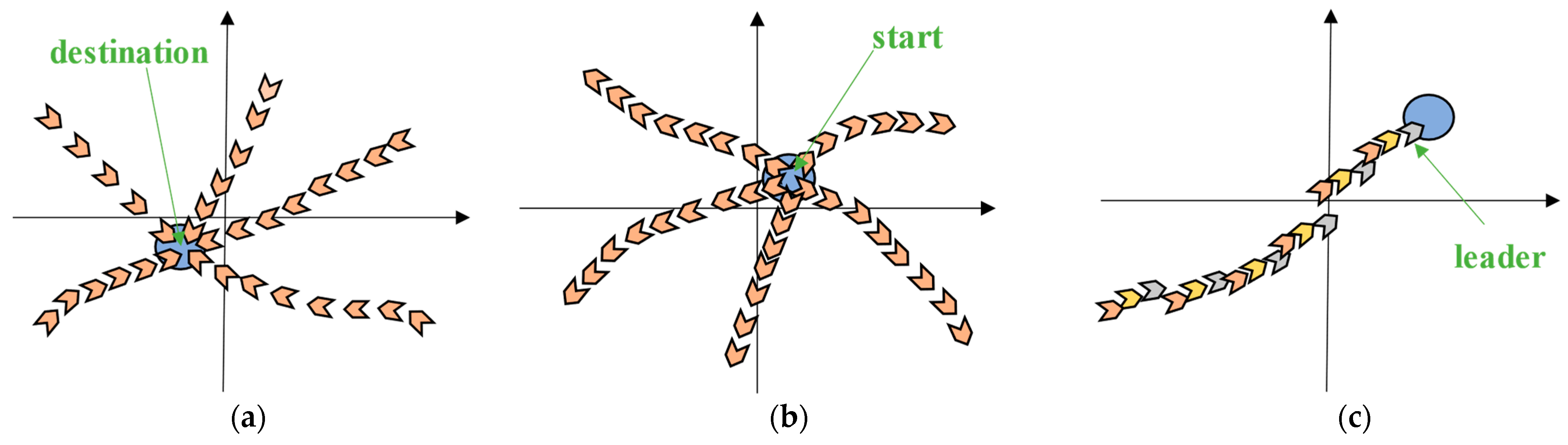
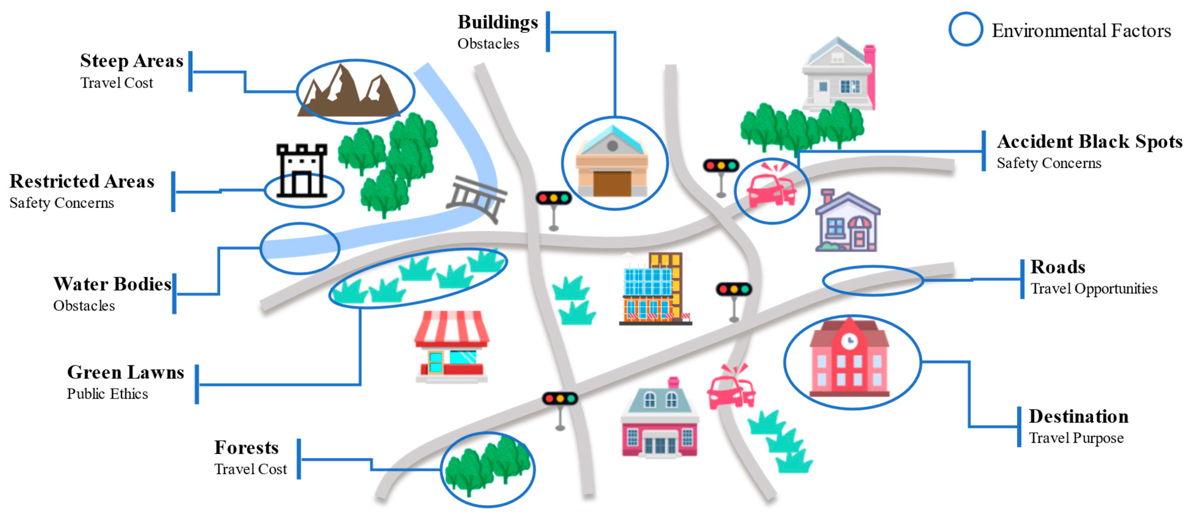
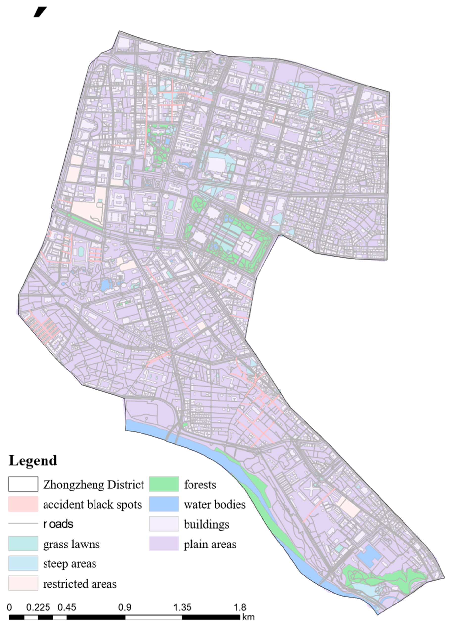
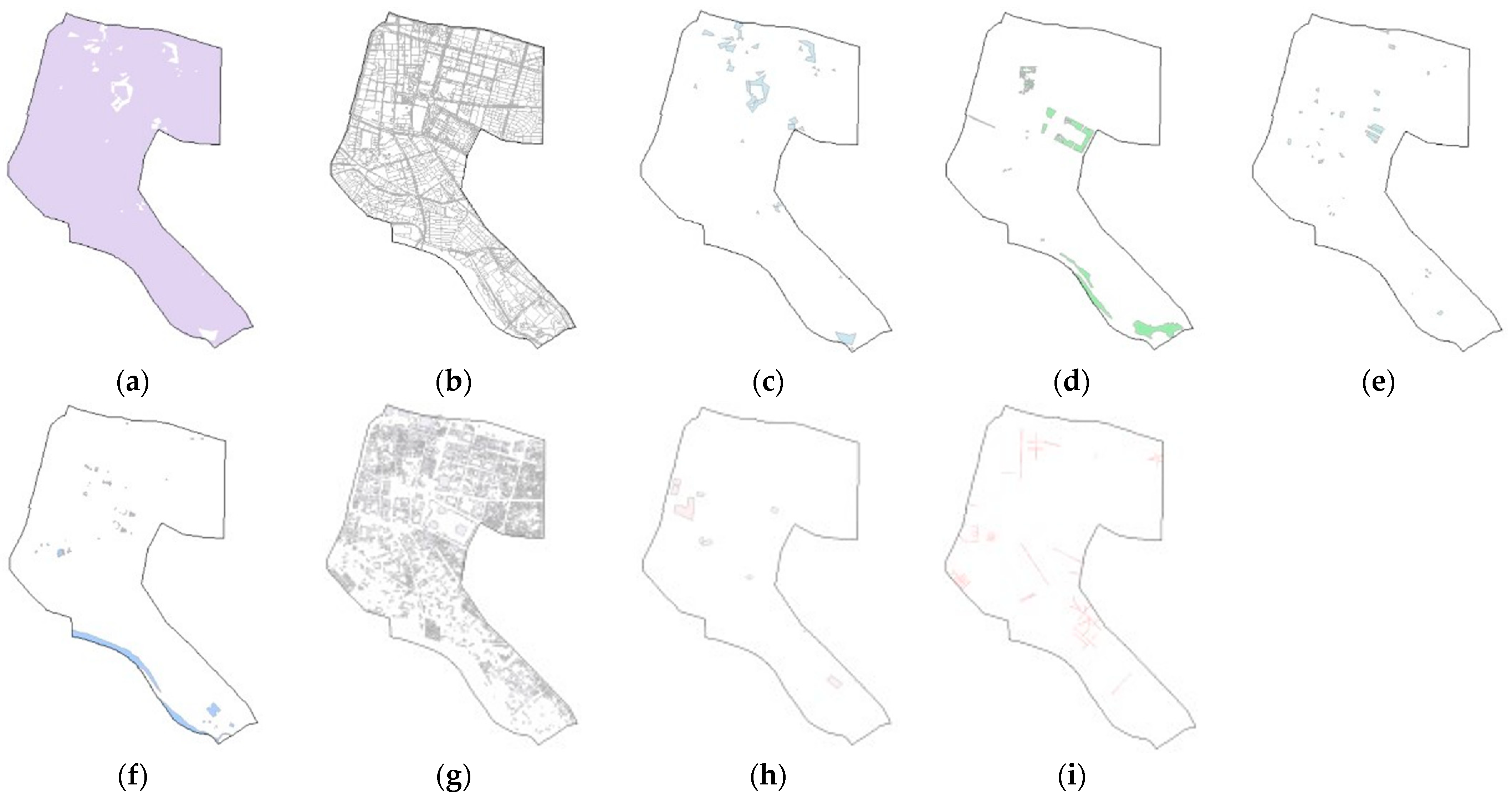

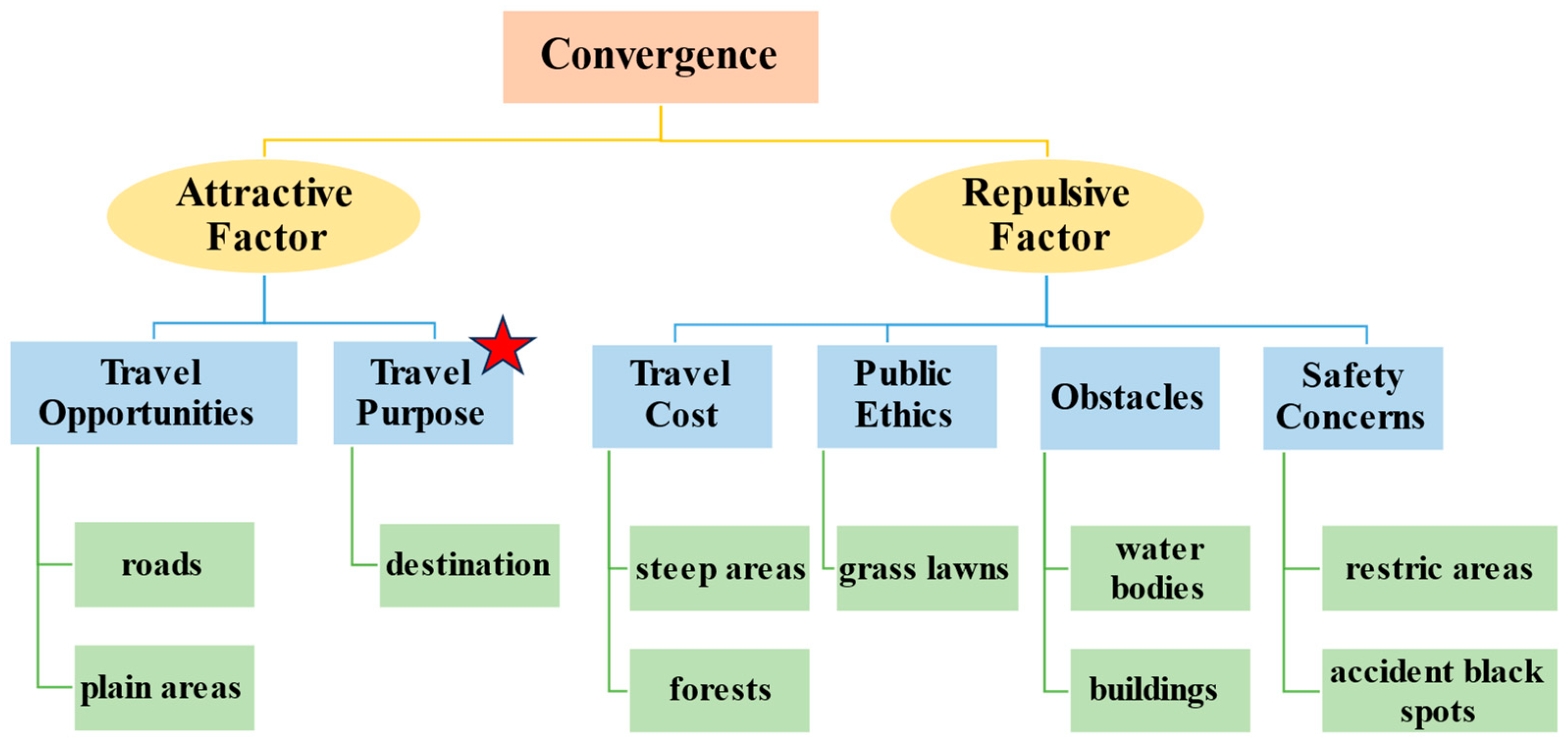

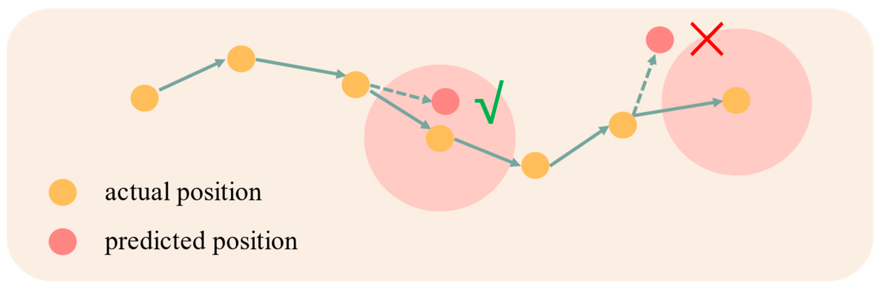
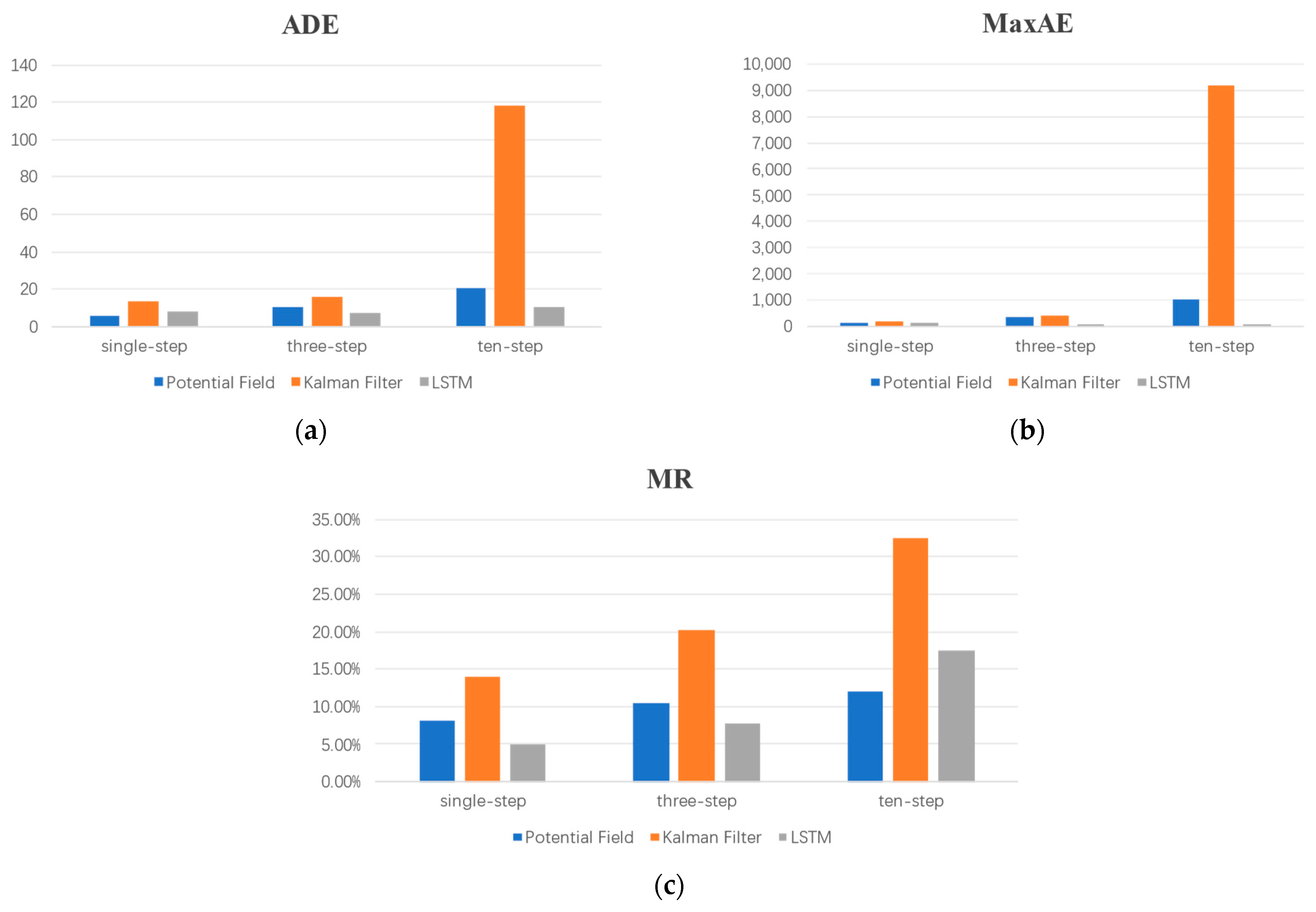
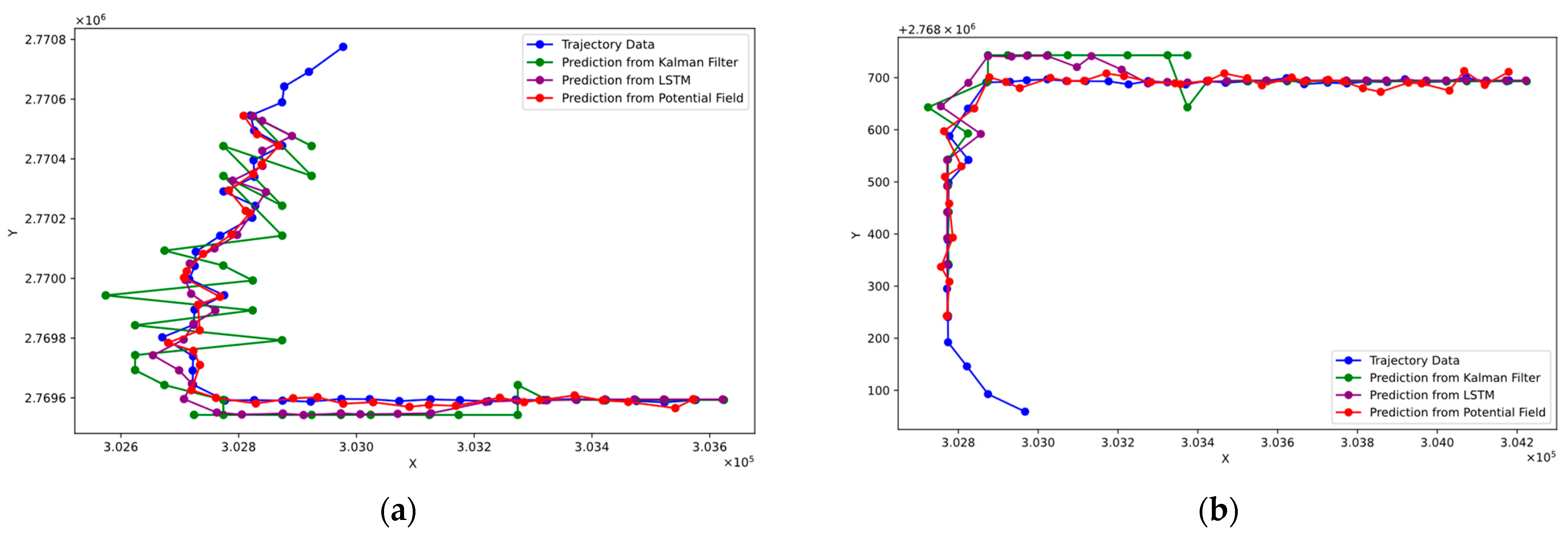


Disclaimer/Publisher’s Note: The statements, opinions and data contained in all publications are solely those of the individual author(s) and contributor(s) and not of MDPI and/or the editor(s). MDPI and/or the editor(s) disclaim responsibility for any injury to people or property resulting from any ideas, methods, instructions or products referred to in the content. |
© 2025 by the authors. Licensee MDPI, Basel, Switzerland. This article is an open access article distributed under the terms and conditions of the Creative Commons Attribution (CC BY) license (https://creativecommons.org/licenses/by/4.0/).