Machine Learning-Based Carbon Emission Predictions and Customized Reduction Strategies for 30 Chinese Provinces

Abstract

With the intensification of global climate change, the discerning identification of carbon emission drivers and the accurate prediction of carbon emissions have emerged as critical components in addressing this urgent issue. This paper collected carbon emission data from Chinese provinces from 1997 to 2021. Machine learning algorithms were applied to identify province characteristics and determine the influence of provincial development types and their drivers. Analysis indicated that technology and energy consumption had the greatest impact on low-carbon potential provinces (LCPPs), economic growth hub provinces (EGHPs), sustainable growth provinces (SGPs), low-carbon technology-driven provinces (LCTDPs), and high-carbon-dependent provinces (HCDPs). Furthermore, a predictive framework incorporating a grey model (GM) alongside a tree-structured parzen estimator (TPE)-optimized support vector regression (SVR) model was employed to forecast carbon emissions for the forthcoming decade. Findings demonstrated that this approach provided substantial improvements in prediction accuracy. Based on these studies, this paper utilized a combination of SHapley Additive exPlanation (SHAP) and political, economic, social, and technological analysis—strengths, weaknesses, opportunities, and threats (PEST-SWOTs) analysis methods to propose customized carbon emission reduction suggestions for the five types of provincial development, such as promoting low-carbon technology, promoting the transformation of the energy structure, and optimizing the industrial structure.

1. Introduction

As global climate change intensifies, the excessive emission of greenhouse gases has caused irreversible damage to the Earth’s ecological environment. Among the more than 30 known greenhouse gases that contribute to global warming, carbon dioxide (CO₂) is the most influential one [1]. Consequently, the mitigation of CO₂ emissions represents an essential challenge on a global scale. As the globe’s second-largest economy, China, responsible for approximately one-third of worldwide CO₂ emissions, emerges as a pivotal actor in international climate regulation. The Chinese government has established ambitious objectives aiming to reach peak carbon emissions by 2030 and attain carbon neutrality by 2060 [2]. These goals not only reflect China’s commitment to global climate responsibility but also provide a clear direction for the country’s development in the coming decades.

However, attaining carbon reduction goals necessitates a profound analytical approach and precise forecasting tailored to the distinct economic development stages, industrial compositions, and energy usage patterns of China’s provinces [3]. Although the existing carbon emission reduction strategies have achieved some results, there is still a lack of regional pertinence, a lack of data accuracy, a neglect of multiple multicollinearities, and a lack of dynamic adjustment mechanism [4,5,6,7]. These deficiencies highlight the need for more precise analysis tools to support scientific and rational measures to reduce emissions and promote sustainable development in various regions [8]. Consequently, the principal aim herein is to pinpoint pivotal determinants of carbon emissions and to construct high-fidelity forecasting models. This endeavor seeks to furnish a robust scientific foundation for the formulation of precisely targeted emission reduction policies.

Within the realm of carbon emission studies, scholars have been dedicated to analyzing the driving factors behind carbon emissions. Regarding the analysis of carbon emission drivers, various models and methods have been employed to investigate how different factors influence emissions. For example, Wang et al. [9] used the Stochastic Impacts by Regression on Population, Affluence, and Technology (STIRPAT) model to scrutinize the determinants of carbon emissions in Jiangsu Province. They concluded that population size, wealth level, technological advancement, urbanization, and industrial structure had significant impacts on carbon emissions. Although the STIRPAT model can assess the comprehensive influence of multiple factors to provide important reference points for policy making on carbon emissions from a macro perspective, it may not capture the complexities and nonlinearities in real-world scenarios fully. To address these limitations, Wei et al. [10] combined the Tapio decoupling model with the STIRPAT model to analyze the carbon emission in rural area drivers comprehensively, revealing that rural urbanization rates and per capita consumption expenditure had negative impacts on carbon emissions, while carbon intensity and total agricultural machinery power had positive effects. In addition to traditional economic models, many scholars have used statistical learning methods to analyze the carbon emissions drivers. For example, Zhao et al. [11] identified per capita GDP as the pivotal determinant of carbon emission disparities in the Yellow River Basin via Quadratic Assignment Procedure Regression analysis. Meanwhile, Dai et al. [12] utilized the resistance model to analyze the major obstacles to industrial carbon reduction in Bengbu City, identifying the urbanization rate as the most significant factor influencing industrial carbon emissions. Yan et al. [13] utilized the Carbon Kuznets Curve approach to ascertain that developed nations attained their peak carbon emissions at an earlier stage. To analyze the contribution of various factors more precisely, many scholars have adopted the Logarithmic Mean Divisia Index (LMDI) method for factor analysis in recent years. Zou et al. [14] established that carbon intensity and energy intensity are critical factors impacting variations in peak carbon emissions within China’s residential building sector through the application of the LMDI model. Building on Zou’s research, Zhang [15] further combined the Kaya identity with the LMDI model to study carbon emission growth in Shandong Province’s construction industry. The Kaya identity is a method used to analyze CO₂ emissions at a national or regional level, attributing changes in emissions to shifts in population, economic activity, energy efficiency, and technological progress [16]. Utilizing this integrated framework, Zhang elucidated that enhancements in residents’ affluence and the quality of building services constitute the principal catalysts for the increase in carbon emissions within Shandong’s construction sector. Carbon emissions are the result of multiple complex factors interacting in intricate, non-linear relationships.

Carbon emissions result from the complex interplay of multiple factors, necessitating a comprehensive analysis from various dimensions. The drivers of carbon emissions vary significantly across regions and industries, necessitating targeted and detailed analyses. Although the STIRPAT model can assess the combined impact of multiple factors from a macro perspective and provide important policy reference points, it may fall short of capturing the full complexity and non-linear relationships inherent in real-world conditions [17]. Furthermore, existing models frequently fail to adequately address the interactions among multiple factors, leading to the omission or underestimation of crucial drivers. Current research has identified several key drivers of carbon emissions and can capture simple non-linear relationships. Additionally, various regression models have been developed to analyze the impacts of these factors and to explain the interactions among them.

In terms of carbon emission forecasting, scholars primarily use two categories of models: statistical models and machine learning models. Among statistical approaches, GM is favored for its effectiveness in small-sample forecasting. For example, Yu et al. [18] used a grey model to predict China’s CO₂ emission trends, indicating that China was expected to achieve zero growth in CO₂ emissions by 2023. However, as a univariate forecasting tool, the GM struggles with capturing interactions among multiple variables, potentially impacting its predictive accuracy and stability. Sapnken et al. [19] proposed an optimized wavelet transform multivariate GM for predicting carbon emissions from road traffic fuel combustion, further improving forecasting accuracy. The autoregressive integrated moving average model is another commonly used statistical model. Zhong et al. [20] developed an integrated forecasting approach combining Empirical Mode Decomposition, autoregressive integrated moving average model (ARIMA), and Truncated Singular Value Decomposition techniques. Also, Ye et al. [21] built a combined forecasting model by integrating ARIMA with support vector regression, and the results demonstrated superior predictive performance. Within machine learning, neural network models are distinguished by their robust nonlinear fitting capabilities. Chuang Luo’s [22] Multi-Echelon Analysis with Back Propagation model forecasted a declining trend in carbon emissions for Jiangsu’s construction industry over the next five years. However, although Long Short-Term Memory (LSTM) excels at handling time series data, a single LSTM model may struggle to capture the intrinsic drivers of data fully in certain specific scenarios. Jiang et al. [23] addressed this limitation with the Bidirectional Adaptive Selection Long Short-Term Memory (BAS-LSTM) model, integrating Variational Mode Decomposition and Empirical Mode Decomposition for enhanced analysis of historical carbon emission data in smart buildings. On the other hand, considering the challenges LSTM faces with training time and resource consumption when processing large-scale datasets, Niu et al. [24] developed a generalized regression neural network forecasting model optimized by an improved fireworks algorithm. The results predicted that China’s total carbon emissions would peak around 2030. Furthermore, in the expansive field of machine learning models, scholars continue to enhance the accuracy and efficiency of carbon emission forecasting. Sun et al. [25] proposed a carbon emission forecasting model based on a bacterial foraging optimization algorithm and least-squares support vector machine, demonstrating significant improvements in prediction accuracy.

While univariate models excel in small-sample predictions, they inadequately capture interactions among multiple variables [26]. While multivariate models better capture the interactions within the data, they require more data and incur higher computational costs. Classical models like ARIMA and support vector machines (SVMs), despite their efficacy on particular datasets, show restricted adaptability and generalizability across varying datasets or time frames [27]. Furthermore, the lack of interpretability in many advanced models restricts their utility in decision making and policy development. Presently, ensemble learning methods are being employed to bolster model robustness and generalization. Additionally, adaptive models are under development, designed to dynamically modify their parameters and structures in response to input data variations. This adaptability equips these models to adeptly handle challenges arising from diverse datasets or time periods.

Despite extensive scholarly research on carbon emission drivers, have targeted and detailed analyses been conducted to address regional disparities? Have the complex non-linear relationships among carbon emission drivers been adequately captured? Have scholars thoroughly elucidated interactions among multiple factors to prevent the omission or underestimation of critical drivers? Concerning carbon emission predictions, have scholars maximized the benefits of hybrid models? Have they improved the interpretability of carbon emission prediction models and incorporated tailored emission reduction and development strategies for various regions?

In summary, this paper focused on analyzing emission reduction strategies at the provincial level in China, aiming to address the limitations of existing research. This paper employed an adaptive K-means++ algorithm to categorize China’s 30 provinces, providing a reliable foundation for regional policy making. By combining Least Absolute Shrinkage and Selection Operator (Lasso) regression with Projection Pursuit Regression (PPR), this paper identified key drivers of carbon emissions across different province types, capturing complex non-linear relationships and interactions among multiple factors, ensuring critical drivers were neither omitted nor underestimated. This paper integrated GM and SVR techniques to predict carbon emissions from 2022 to 2032. The resulting grey model–support vector regression (GM-SVR) hybrid model significantly enhanced prediction accuracy and generalization performance. To improve model transparency and interpretability, the SHAP framework was introduced. This increased the explainability of the predictive model, offering policymakers more intuitive and reliable insights. Through PEST-SWOT analysis, this paper explored heterogeneity among different categories, providing practical support and tailored policy recommendations for emission reduction and development strategies specific to each type of province.

This paper comprises five sections. Section 2 provides a brief summary of the materials and methods. Section 3 summarizes the implementation of machine-learning classification, selection, and heterogeneity of driving factors and the findings from the carbon emission prediction model. Section 4 describes the regional heterogeneity analysis for the five types of provinces and provides tailored carbon emission reduction suggestions for each type of provincial development. Finally, Section 5 presents the research conclusions.

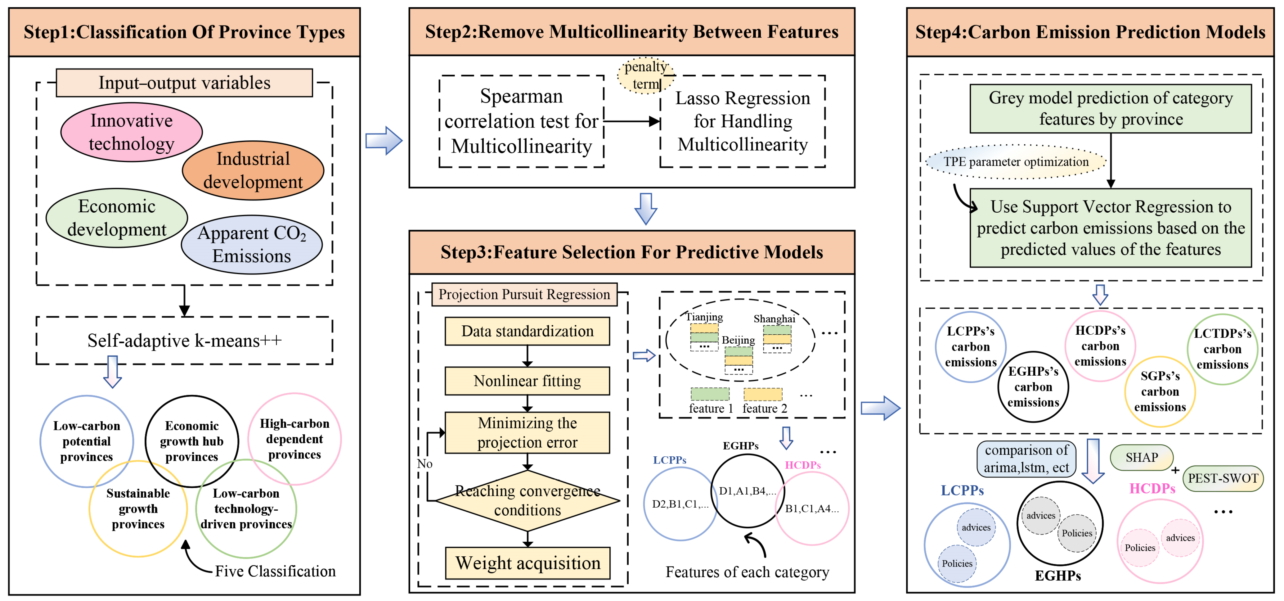
2. Materials and Methods

In this section, this paper proposed a combined machine learning model integrating category classification, driver selection, and prediction. An adaptive K-means++ algorithm was used to cluster provinces into distinct groups based on four key driving factors. The Spearman correlation coefficient detected multicollinearity among the driving factors, which was then resolved using Lasso regression. PPR further filtered the driving factors within each category. For carbon emission forecasting, the GM model was used to predict the driving factors initially. Based on the GM results, SVR was applied to predict carbon emissions for provinces within each category. Eventually, the SHAP and PEST-SWOT algorithms were used to analyze the prediction results and provide policy recommendations for each category. In this paper, Python 3.6 was used to program for the algorithms and data analysis. In addition, the experimental data were plotted and visualized using Origin 2021. The algorithm structure is shown in Figure 1.

2.1. Province Clusters

2.1.1. Classification Data Processing

This paper selected four driving factors as classification criteria for the provinces: per capita GDP, technological market transaction volume, carbon dioxide emissions, and the proportion of secondary industry in GDP. Green et al. [28] identified carbon dioxide emissions as a critical metric for assessing environmental impact and guiding sustainable development goals. Wang et al. [29] emphasized that the contribution rate of the secondary industry to GDP signifies the extent of industrial development. Both Wang, Q. et al. and Wang, Y. et al. [30,31] argued that per capita GDP serves as a proxy for human capital and is a key indicator for measuring the sustainable economic development capacity of cities. Zhou et al. [32] highlighted that the volume of transactions in the technology market plays a pivotal role in fostering technological innovation. Given that categorical variables fluctuated over time, they led to the same province being classified into different categories at different time points. To overcome this issue, this paper adopted the time-weighted variable method to transform panel data into cross-sectional data, ensuring that the same province maintained consistent classification throughout the entire study period. The formula for the time-weighted variable method is shown in Equation (1):

$$W_{S_i}=\sum {\displaystyle \frac{t-t_{min}+1}{\sum \left(t-t_{min}+1\right)}}\times S_i,$$

(1)

where $W_{S_i}$ represents the weighted classification variable value for the i province, t denotes the current year in the data, $t_{min}$ represents the earliest year in the data, and $S_i$ represents the original classification variable value for the i province at time t.

2.1.2. Self-Adaptive k-Means++ Algorithm

Unsupervised classification models are required to classify individual provinces. Therefore, this paper uses the k-means++ for the classification of provinces. The k-means++ requires the determination of the number of clusters, k, depending on the dataset’s features and previous experience. However, the selection of k has an important effect on the clustering results. An unsuitable k value can directly influence the effectiveness of predictive models. Therefore, this paper improved the k-means++ by including an adaptive determination of k [33,34,35]. This ensures the reliability of classification results and improved accuracy of subsequent predictive models. The pseudocode for self-adaptive k-means++ is visible in Algorithm A1.

The distance formula, the silhouette coefficient calculation, and the formula for determining new cluster centers in the self-adaptive k-means++ algorithm are presented in Equations (2)–(4).

$$d\left(h,c_i\right)=\sqrt{{\displaystyle \sum _{j=1}^n}{(h_j,c_{ij})}^2},$$

(2)

$$u_i={\displaystyle \frac{b_i-a_i}{\mathrm{m}\mathrm{a}\mathrm{x}(a_i,b_i)}},$$

(3)

$$c_i^{\prime }={\displaystyle \frac{1}{\left|S_i\right|}}{\displaystyle \sum _{h\in S_i}}h,$$

(4)

where $d\left(h,c_i\right)$ is the distance matrix of each node to the cluster centers, $u_i$ is the silhouette coefficient for the i cluster with k value, $c_i^{\prime }$ is the matrix of new cluster centers, and $S_i$ is the set of data points in the i cluster.

2.2. Lasso Regression

Lasso regression is an unbiased estimation method used to handle high-dimensional and complex collinear data. The basic idea is to add an L1 norm penalty term to the fitting of a generalized linear regression [36]. Compared to the L2 norm penalty term in Ridge regression, Lasso regression is better at shrinking the coefficients of less important variables to 0. Therefore, it is widely used for dimensionality reduction of driving factors and preventing overfitting. The constructed penalty function is shown in Equation (5):

$${\displaystyle \underset{w}{\min }}{\displaystyle \frac{1}{2n}}{‖y-Xw‖}_2^2+\lambda {‖w‖}_1={\displaystyle \underset{w}{\min }}f\left(x\right)=g(x)+h(x),$$

(5)

where y denotes the carbon emission matrix, X denotes the matrix of driving factors for each province, w denotes the matrix of regression coefficients for the independent variables, and $\lambda$ denotes the regularization coefficient.

The first term in Equation (5) is a differentiable convex function, while the second term is a non-differentiable convex function that satisfies the L-Lipschitz condition. Therefore, the proximal gradient descent method can be used to solve the Lasso regression. In this paper, the penalty function is expanded using the second-order Taylor expansion, and the Lipschitz constant is used to express it.

$$\widehat{f}\left(x\right)\approx {\displaystyle \frac{L}{2}}{‖x_k-\left(x_k-{\displaystyle \frac{1}{L}}\nabla f\left(x_k\right)\right)‖}_2^2+const,$$

(6)

where ${\displaystyle \frac{1}{L}}$ is the iteration step size. By setting $x=x_k-{\displaystyle \frac{1}{L}}\nabla f\left(x_k\right)$, the maximum minimization can be achieved. Therefore, the iteration formula is expressed as Equation (7):

$$x_{k+1}={\displaystyle \frac{L}{2}}{\displaystyle \sum _{i=1}^n}{(x^{\left(i\right)}-{\displaystyle \frac{1}{L}}\nabla f\left(x_k\right))}^2+\lambda {\displaystyle \sum _{i=1}^n}\left|x_i\right|.$$

(7)

The optimization for each dimension of the parameter in Equation (7) is performed separately. Meanwhile, the proximal gradient descent method is used for solving the Lasso regression. The solution obtained is as follows:

$$x=\left\{\begin{array}{c}z+{\displaystyle \frac{\lambda }{L}}, z<-{\displaystyle \frac{\lambda }{L}}\\ 0, \left|z\right|\le {\displaystyle \frac{\lambda }{L}}\\ z-{\displaystyle \frac{\lambda }{L}}, z>{\displaystyle \frac{\lambda }{L}}\end{array}\right..$$

(8)

2.3. Carbon Emission Prediction Algorithm

This paper uses the GM algorithm and TPE Bayesian parameter optimization SVR algorithm to predict carbon emission amounts for each province across different categories.

2.3.1. GM Algorithm

GM is a prediction technique that can provide effective prediction when data is scarce. The core advantage of this method is its ability to build mathematical models and make accurate predictions even with only four data points, addressing the challenge of insufficient historical data [37]. Owing to the individual driving factors for each category of provinces in this paper, which consist of 24 data points, the GM was used to forecast the driving factors for each category. The specific steps of the model are as follows:

Let the original sequence be

$$x^{\left(0\right)}=\left(x^0\left(1\right),x^0\left(2\right),\dots ,x^0\left(n\right)\right),$$

(9)

$$x^{\left(r\right)}\left(k\right)={\displaystyle \sum _i^k}{x}^{\left(r-1\right)}\left(i\right),k=\mathrm{1,2},\dots ,n,$$

(10)

where ${ x}^{\left(r\right)}\left(k\right)$ represents the cumulative generating sequence of the original sequence $x^{\left(0\right)}$ for each category’s driving factor. In this paper’s model $r=1$.

Based on the cumulative generation sequence of the driving factors for each category, the grey differential equation is established and discretized. The formulation is detailed in Equations (11) and (12):

$$z^1\left(k\right)=\left(z^1\left(1\right),z^1\left(2\right),\dots ,z^1\left(n\right)\right),$$

(11)

$$z^1\left(k\right)={\displaystyle \frac{1}{2}}\left(x^1\left(k\right)+x^1\left(k-1\right)\right),$$

(12)

where $z\left(k\right)$ is the adjacent mean generating sequence of the cumulative generating sequence for each category’s driving factor.

Next, based on Equations (11) and (12), this paper uses the least squares method to determine parameters a and b and write them in matrix form. Its matrix form is shown in Equation (13):

$$Y=\left[\begin{array}{c}x\left(2\right)\\ ⋮\\ x\left(n\right)\end{array}\right],B=\left[\begin{array}{cc}-z\left(2\right)& 1\\ ⋮& ⋮\\ -z\left(n\right)& 1\end{array}\right],A=\left[\begin{array}{c}a\\ b\end{array}\right].$$

(13)

By substituting parameters a and b into the differential equation, the prediction equation for the cumulative sequence obtained by summing the driving factors across different categories is obtained, as shown in Equation (14).

$$x\left(k+1\right)=\left(x\left(1\right)-{\displaystyle \frac{b}{a}}\right)e^{-a\left(k-1\right)}-\left(x\left(1\right)-{\displaystyle \frac{b}{a}}\right)e^{-a\left(k-2\right)},$$

(14)

where $x(k+1)$ denotes the predicted value.

2.3.2. SVR Prediction Algorithm with TPE Bayesian Parameter Optimization

Built on the various category eigenvalues obtained by GM prediction, this paper used the SVR prediction algorithm based on TPE Bayesian parameter optimization to predict the carbon emission of each province in each category.

1.

TPE-based Bayesian Parameter Optimization

Bayesian optimization optimizes the objective function by constructing a probabilistic model between hyperparameters and performance. It continuously observes the evaluation results of the objective function and updates the posterior probability distribution of the objective function to reasonably select the next hyperparameter to be evaluated [38]. Because SVR is very sensitive to hyperparameter selection, different hyperparameter settings can lead to significant differences in model performance. Therefore, the Bayesian optimization based on the TPE is used for the hyperparameter tuning of the SVR model. The main steps are as follows:

Each hyperparameter is assumed to follow a Gaussian distribution with a mean of 0 being chosen. n sets of hyperparameters X were randomly sampled and the corresponding true loss y for these hyperparameters was computed. In addition, the TPE procedure was set to fit the proxy function to $X\to y$ and a hyperparameter $\gamma$ was set to represent the quantile of y with a value of 0.25. The formula is expressed as Equation (15):

$$f\left(x\right)=\gamma l\left(x\right)+\left(1-\gamma \right)g\left(x\right).$$

(15)

EI function is chosen to evaluate the acquisition points as the acquisition function. Also, the EI function can represent the average lift level of y relative to threshold $y^{\ast }$ given x. Its formula is shown in Equation (16):

$$E{I}_{y^{\ast }}\left(x\right)={\int }_{-\infty }^{+\infty }\mathit{max}\left(y^{\ast }-y,0\right)P_M\left(\left.y\right|x\right)dy.$$

(16)

Sampling group c group hyperparameters composition $X_{candidate}$. For each $x_i$ in $X_{candidate}$, this paper calculates $P_M\left(\left.y_i\right|x_i\right)$ and selects the optimal $x^{\ast }$ from the acquisition points. Then, this paper inputs it into the model to compute the actual loss $y^{\ast }$, as shown in Equations (17) and (18).

$$E{I}_{y^{\ast }}\left(x\right)={\int }_{-\infty }^{y^{\ast }}\left(y^{\ast }-y\right){\displaystyle \frac{l\left(x\right)p\left(y\right)}{\gamma l\left(x\right)+\left(1-\gamma \right)g\left(x\right)}}dy,$$

(17)

$$E{I}_{y^{\ast }}\left(x\right)={\displaystyle \frac{{\int }_{-\infty }^{y^{\ast }}\left(y^{\ast }-y\right)p\left(y\right)dy}{\gamma +\left(1-\gamma \right)\frac{g\left(x\right)}{l\left(x\right)}}}.$$

(18)

From Equation (18), it can be seen that the value of the EI function is proportional to the inverse of its denominator. Once $\gamma$ is determined, the size of the denominator depends on the ratio of the probabilities at both ends of ${\displaystyle \frac{l\left(x\right)}{g\left(x\right)}}$. Therefore, the optimal acquisition point is the one that maximizes this ratio.

2.

SVR

SVR is a regression method based on the principles of SVM. The core idea is to find an optimal hyperplane or a non-linear function that can predict the continuous output values as accurately as possible [39]. Compared to traditional regression methods, SVR handles non-linear problems by introducing a loss function and kernel tricks, while also controlling the complexity of the model to avoid overfitting. Therefore, this paper used the SVR model to predict the carbon emissions of different categories of provinces.

The SVR model defines a “tolerance band” through an $ϵ-insentiveloss$ loss function. The loss is only included when the deviation between the predicted value of carbon emissions and the true value of carbon emissions of each province exceeds ε, as shown in Equation (19).

$$L_{\epsilon }\left(y,f\left(x\right)\right)\left\{\begin{array}{c}0, \left|y-f\left(x\right)\right|\le \epsilon \\ \left|y-f\left(x\right)\right|-\epsilon , else\end{array}\right.,$$

(19)

where $\epsilon$ represents a preset tolerance threshold. When the prediction error is within $\epsilon$, the loss is zero. When the prediction error exceeds $\epsilon$, the loss is the prediction error minus $\epsilon$. $f\left(x\right)$ is the predicted carbon emission value for each category of provinces, and y is the actual carbon emission value for each category of provinces.

The objective of SVR is to minimize the deviation between the predicted and actual carbon emission values for each category of provinces. This can be expressed as Equation (20):

$${\displaystyle \underset{w,b,\xi ,{\xi }^{\ast }}{\mathit{min}}}{\displaystyle \frac{1}{2}}{‖w‖}^2+C{\displaystyle \sum _{i=1}^n}\left({\xi }_i+{\xi }_i^{\ast }\right),$$

(20)

where ${\xi }_i$ and ${\xi }_i^{\ast }$ are slack variables representing the deviation beyond the $\epsilon$ insensitive error tolerance, and C is the penalty coefficient used to balance the model’s complexity and smoothness.

2.4. Data Sources and Selection

2.4.1. Data Sources

The data used in this paper covered carbon emissions in China’s provinces from 1997 to 2021. These data were sourced from the China Emission Accounts and Datasets (CEADs) [40,41,42,43,44], accessible at https://www.ceads.net/data/province/ (accessed on 1 October 2024). Carbon emission driving factors were obtained from the China Provincial Statistical Yearbook for the period of 1997 to 2021. For missing data, this paper referred to the China Environmental Yearbook, China Science and Technology Statistical Yearbook, China Railway Yearbook, and official websites of provincial statistical bureaus for supplementation and completion.

2.4.2. Data Selection

Previous literature indicated that carbon emissions were related to multiple domains closely, including social development, energy economy, and the environment [45,46,47]. Therefore, this paper considered 23 relevant driving factors comprehensively, categorizing them into five main categories systematically: population, economy, society, energy, and environment. The driving factor system is presented in

Table 1. Driving Factor System.

Primary Feature	Secondary Feature	Unit	Code
Population	Total Population	Ten thousand people	A1
	Urbanization Rate	%	A2
	Urban Population	Ten thousand people	A3
	Resident Population at Year-End	Ten thousand people	A4
Economy	Proportion of Secondary Industry in GDP	%	B1
	Proportion of Tertiary Industry in GDP	%	B2
	GDP per Capita	CNY	B3
	Gross Regional Product	Hundred million CNY	B4
	GDP per Capita of Region	CNY/person	B5
Social Factors	Technology Market Transaction Value	Ten thousand CNY	C1
	Road Passenger Traffic	Ten thousand CNY	C2
	Rail Passenger Traffic	Ten thousand CNY	C3
	Passenger Traffic	Ten thousand passenger trips	C4
	Education Expenditure	Ten thousand CNY	C5
	Domestic Patent Applications Received	Items	C6
Energy Factors	Carbon Dioxide Emissions	MT	D1
	Coal Consumption	Ten thousand tons	D2
	Gasoline Consumption	Ten thousand tons	D3
	Natural Gas Consumption	Hundred million cubic meters	D4
	Diesel Consumption	Ten thousand tons	D5
	Electricity Consumption	Billion kWh	D6
	Kerosene Consumption	Ten thousand tons	D7
Environmental Factors	Green Coverage Rate in Built-up Areas	%	E1

.

3. Results

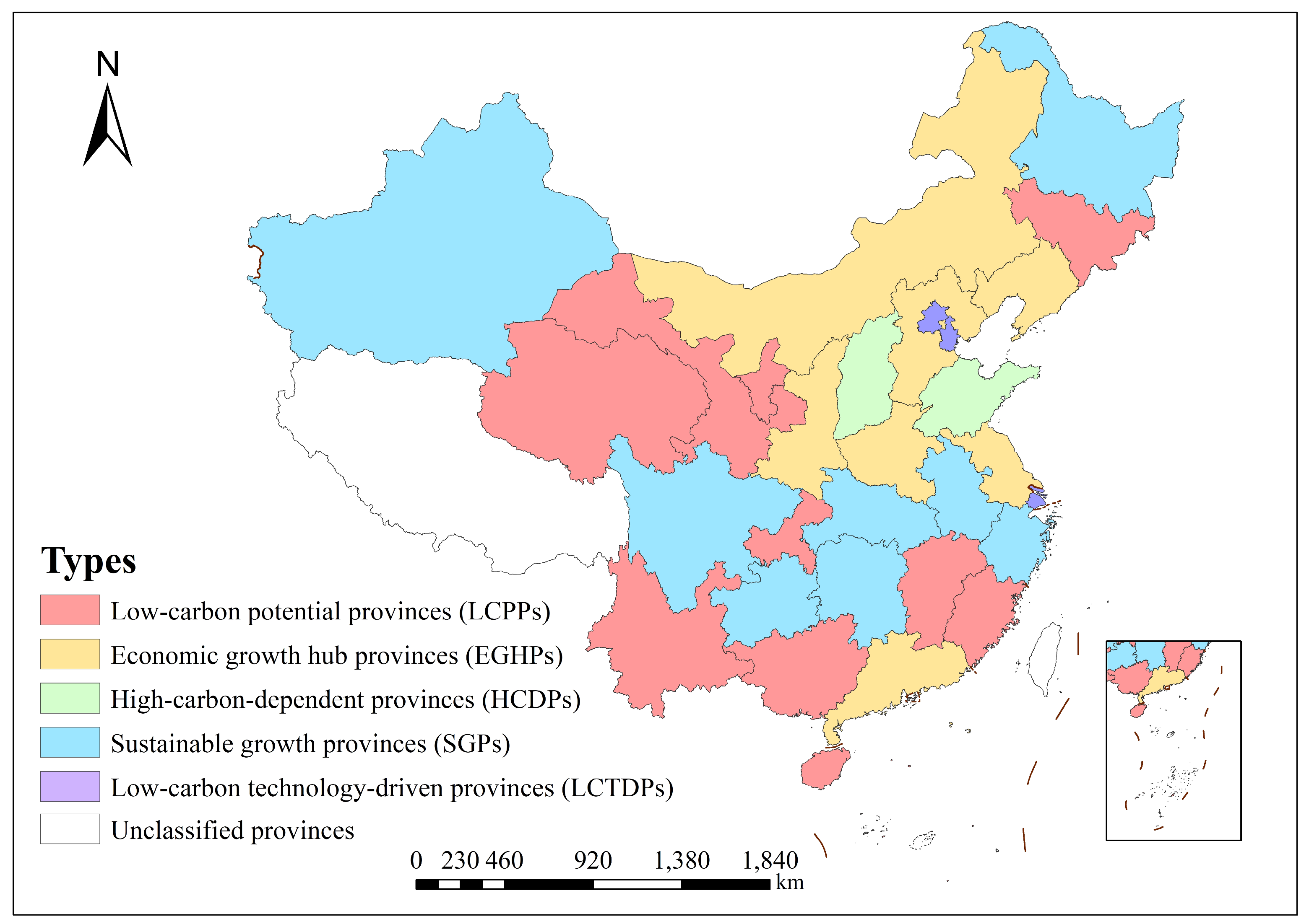
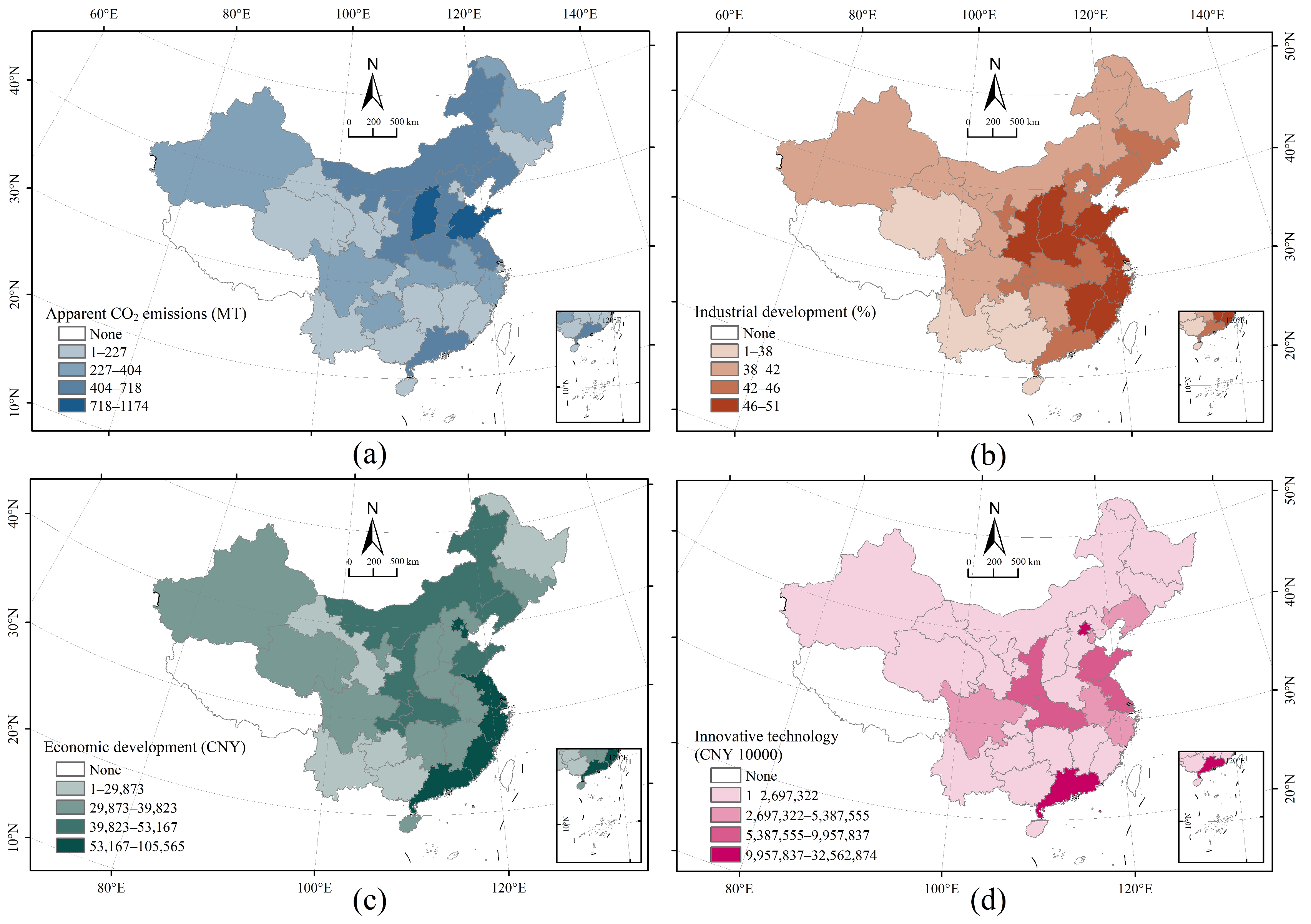
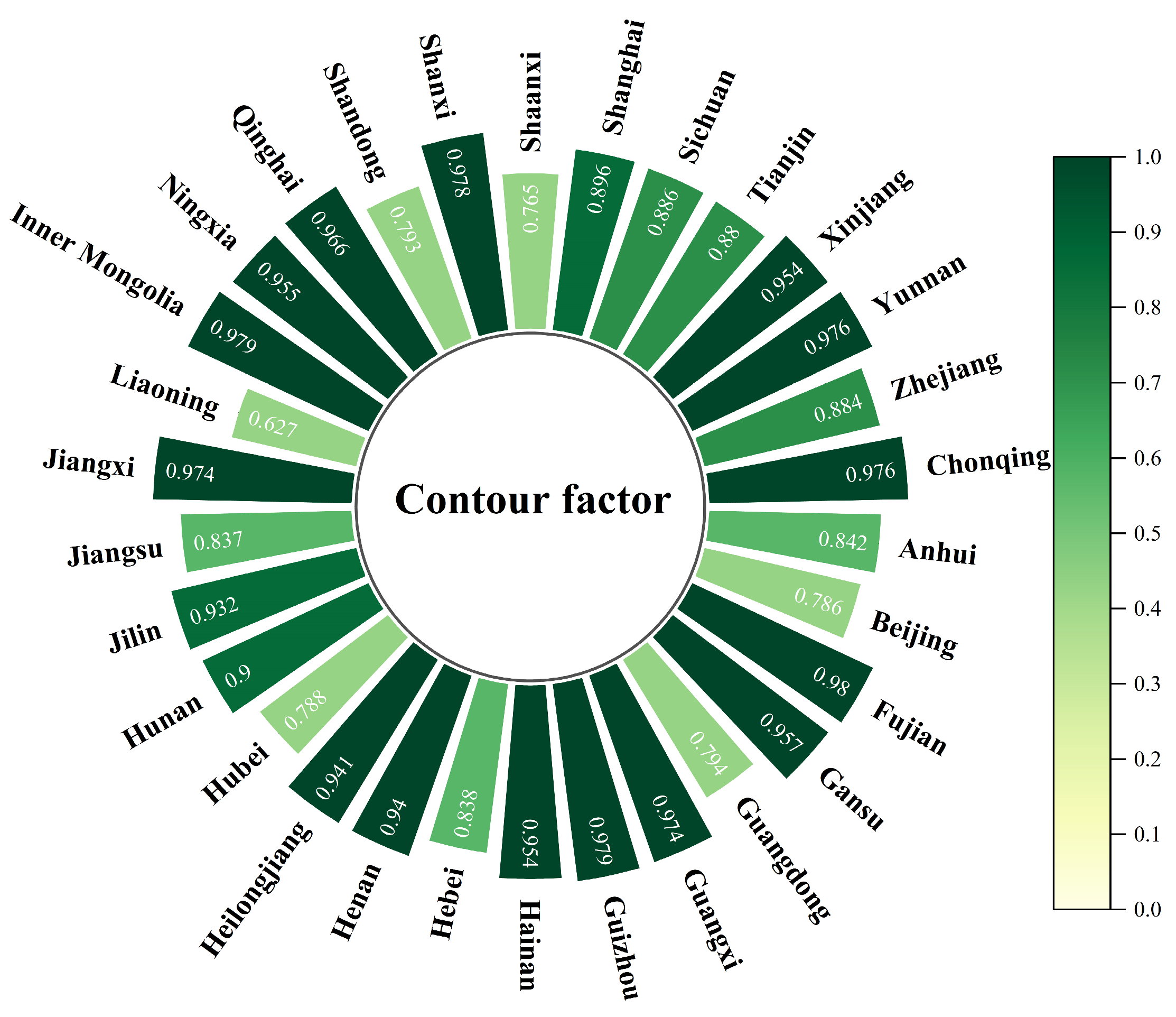
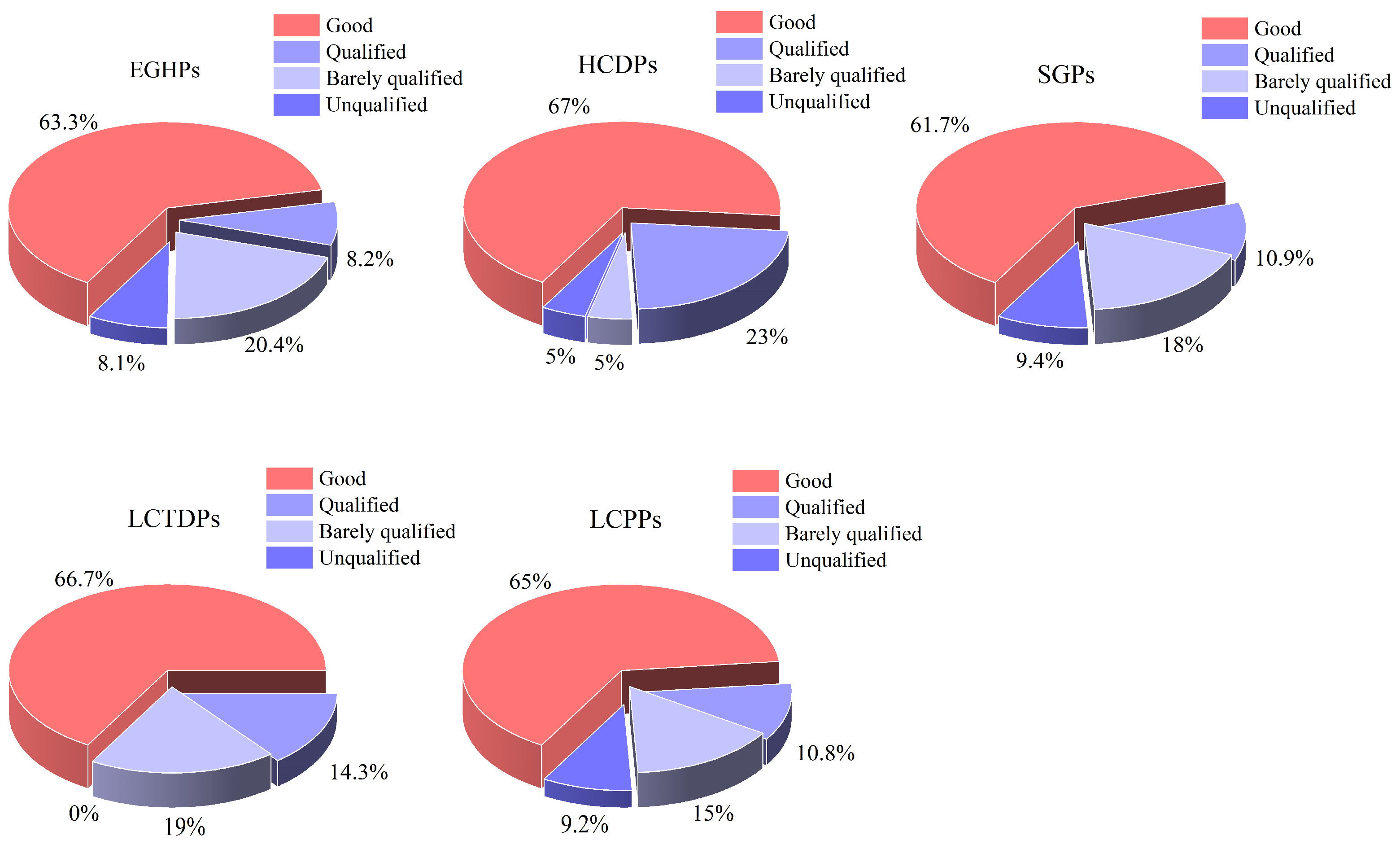
3.1. Provincial Classification

Based on the classification data processed by the time-weighted variable method, this paper used an adaptive k-means++ clustering approach to categorize the 30 provinces into 5 distinct groups: EGHPs, HCDPs, SGPs, and LCTDPs. Clustering results are shown in Figure 2.

As shown in Figure 2, EGHPs are located in central and eastern regions, including Shaanxi, Inner Mongolia, Liaoning, Jiangsu, Henan, Hebei, and Guangdong. HCDPs, concentrated in the eastern and northern regions, consisted of Shanxi and Shandong. SGPs, distributed across various regions nationwide, encompassed Zhejiang, Xinjiang, Sichuan, Hunan, Hubei, Heilongjiang, Guizhou, and Anhui. Meanwhile, LCTDPs are centered in major cities, including Tianjin, Shanghai, and Beijing. Finally, the remaining provinces were classified as LCPPs.

Spatial Distribution of Four Driving Factors

To further explore the spatial distribution of the four driving factors, this paper visualized the spatial distribution of the factors, as shown in Figure 3.

As shown in Figure 3, EGHPs exhibited high per capita GDP and vibrant technological market transactions. These provinces achieved a balance between economic growth and environmental protection through the optimization of industrial structures and technological advancements. HCDPs were characterized by significant industrial contributions to GDP and substantial carbon dioxide emissions, yet they showed relatively low technological market activity. Transitioning towards cleaner energy sources has been crucial for these provinces to reduce their carbon footprint. SGPs emphasized green technologies and renewable energy, maintaining low carbon emissions and a balanced proportion of secondary industry within GDP. LCTDPs prioritized high-technology innovation, boasting the highest levels of technological market transactions and the lowest carbon emissions. Finally, LCPPs lagged in economic and technological development but possessed abundant natural resources and significant potential for advancing low-carbon economies.

To validate the performance of the algorithm, this paper visualized the silhouette coefficients of the samples. The silhouette coefficients for the adaptive k-means++ clustering are shown in Figure 4.

As shown in Figure 4, the silhouette coefficients of most provinces ranged from 0.79 to 0.98, indicating that the overall clustering effect was good, and the province classification was significant. This proved the effectiveness of the adaptive k-means++ clustering method in province classification.

3.2. Handling Multicollinearity

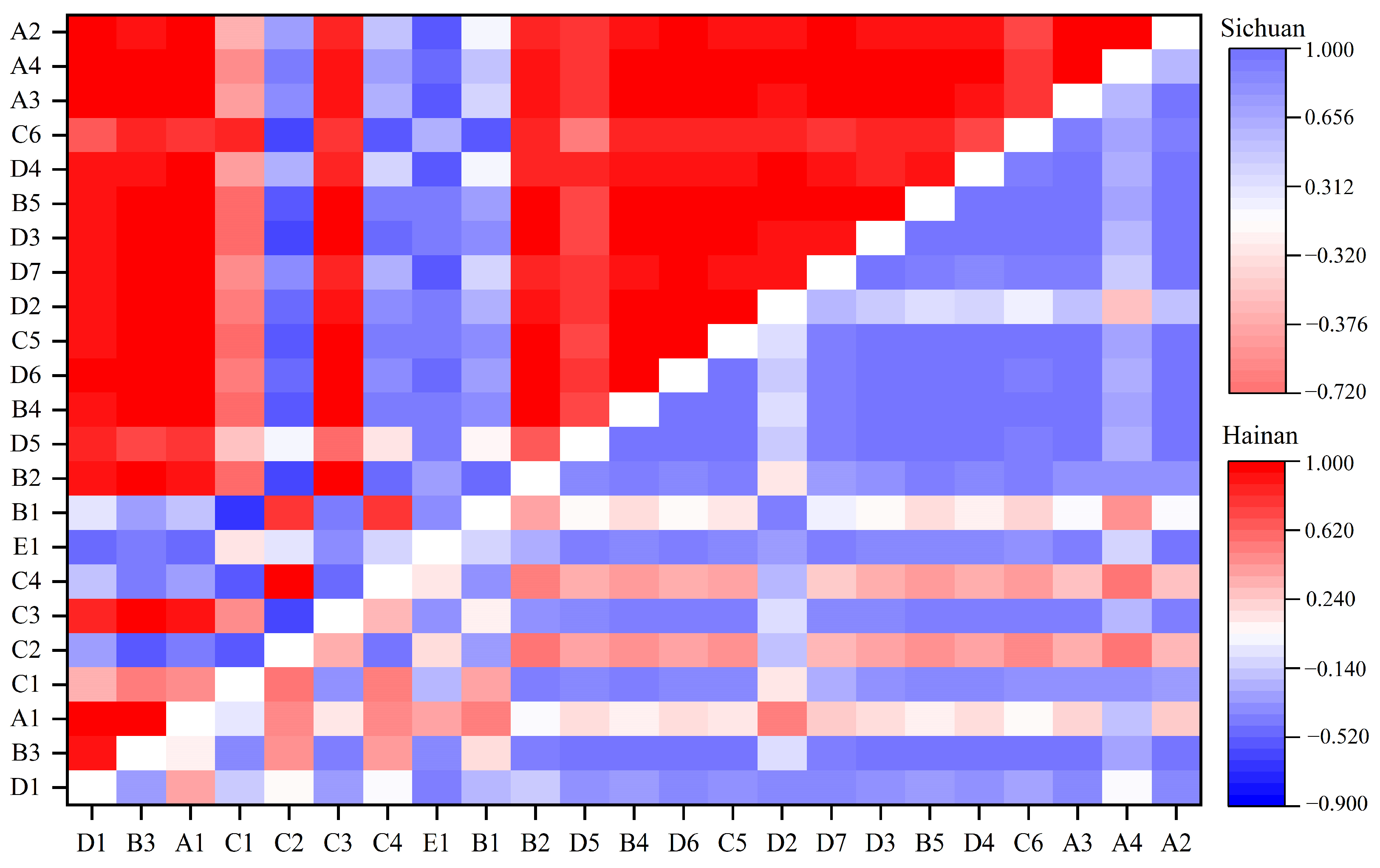
3.2.1. Multicollinearity Analysis of the Driving Factors

Given that the dataset of each province contained 23 driving factors, the dataset exhibited a multidimensional and complex correlation structure. This paper used Spearman correlation analysis to detect multicollinearity among the driving factors, as shown in Figure 5.

As shown in Figure 5, the correlation coefficients between some driving factors were close to 1, indicating that there was multicollinearity among the driving factors.

3.2.2. Lasso Regression to Address Multicollinearity

Given the multicollinearity among some driving factors in the dataset of each province, this paper treated the driving factors of each province as independent variables and carbon dioxide emissions as the dependent variable. Based on standardized data, this paper employed cross-validation methods to select the optimal penalty parameter for each province. After calibrating the optimal penalty parameter through cross-validation, this paper obtained the Lasso regression coefficients for the driving factors of each province. The Lasso regression coefficients for the driving factors of some provinces are shown in

Table 2. Lasso Regression Coefficients for Driving Factors of Selected Provinces.

Province	B3	A1	C1	C2	C3	C4	E1
Shanghai	0.006	−0.023	0	−0.01	−0.008	0	0.319
Yunnan	0	−0.292	0	0	0.005	−0.001	−0.404
Inner Mongolia	0.037	0.794	0	−0.023	0.041	0.022	−0.675
Beijing	0	0.059	0	0	0.001	0	−0.303
Jilin	0.001	0.234	0	−0.006	−0.001	0.006	0.101
Sichuan	−0.001	−0.046	0	−0.002	−0.002	0.002	−4.88
Tianjin	−0.003	0	0	0.028	0.039	−0.028	0
Ningxia	0.003	3.242	0	−0.02	0.053	0.018	1.854
Anhui	−0.006	−0.041	0	0.004	0.011	−0.004	−0.61
Shandong	0.026	1.441	0	−0.003	0.009	0.003	4.257
Shanxi	−0.384	−0.576	0.001	0.127	0.176	−0.155	−19.819
Guangdong	0	−0.017	0	0.001	0	−0.001	−2.114
Guangxi	0.006	−0.027	0	0.004	0.005	−0.003	0.076
Xinjiang	0.01	−0.039	0	0	−0.002	0	2.185
Jiangsu	0	−0.625	0	−0.005	−0.006	0.005	−0.761
Jiangxi	0.001	−0.098	0	−0.001	0	0.001	−0.299
Hebei	−0.094	0.772	0	0	0.02	−0.001	0
Henan	−0.05	0.125	0	−0.021	−0.03	0.02	0.19
Zhejiang	0.01	−0.011	0	0.011	0.01	−0.011	2.707
Hainan	−0.002	−0.222	0	−0.012	−0.02	0.012	0.139
Hubei	−0.001	−0.008	0	0	0.003	0	−0.453
Hunan	0.005	0.142	0	0	−0.001	0	−11.551
Gansu	−0.002	−0.019	0	0.004	0.007	−0.004	0.306
Fujian	0.004	−0.069	0	0.001	0	−0.001	−3.901
Guizhou	0.02	0.02	0	0	−0.019	0	−0.809
Liaoning	−0.064	0.344	0	0.009	0.004	−0.008	0.254
Chongqing	−0.002	−0.126	0	0	0.013	0	−1.078
Shaanxi	0.016	2.562	0	0.012	0.021	−0.012	−1.566
Qinghai	0.007	0.418	0	−0.015	0.007	0.015	−0.24
Heilongjiang	−0.004	0.399	0	−0.002	0.016	0	0.04

.

As shown in Table 2, the B3 factor exhibited a positive effect on carbon emissions in provinces such as Shanghai, Inner Mongolia, and Jilin. Conversely, the A1 factor was found to significantly reduce carbon emissions in most provinces, with particularly notable effects observed in Ningxia and Shandong. The E1 factor displayed substantial negative coefficients across numerous provinces, underscoring its critical role in mitigating carbon emissions. In contrast, the C1 to C4 factors were nearly zero across the dataset for all provinces, indicating that these variables are highly collinear with other factors within specific regions. Consequently, Lasso regression effectively addresses these multicollinearity issues through its distinctive L1 regularization mechanism, thereby enhancing the model’s robustness and interpretability.

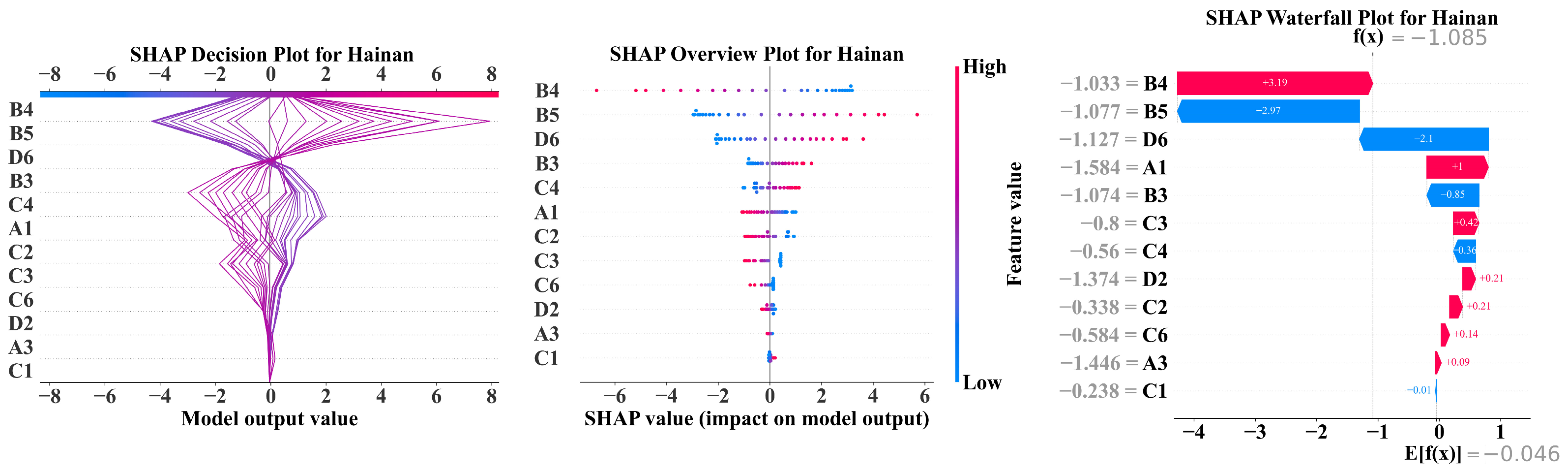
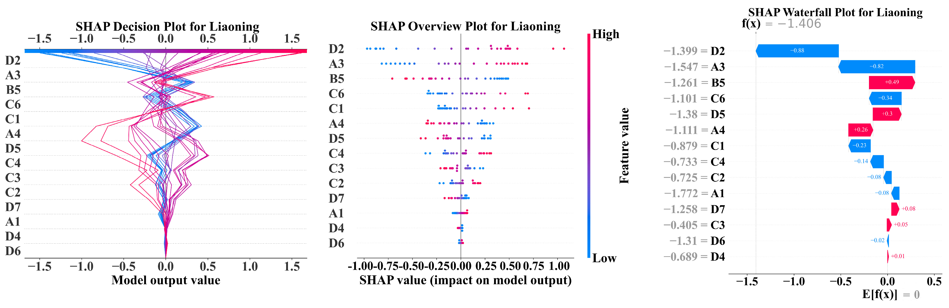
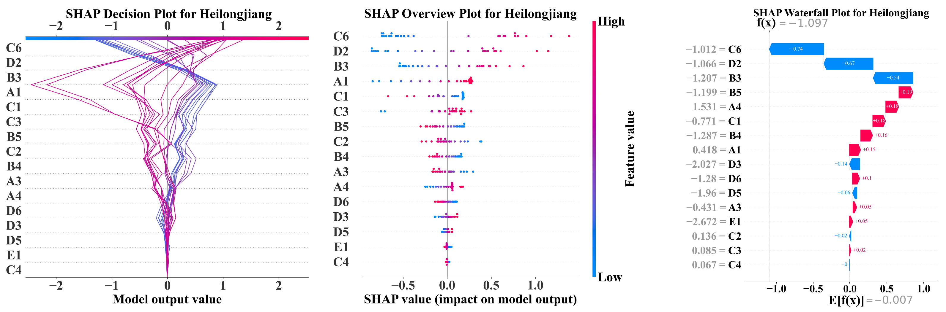
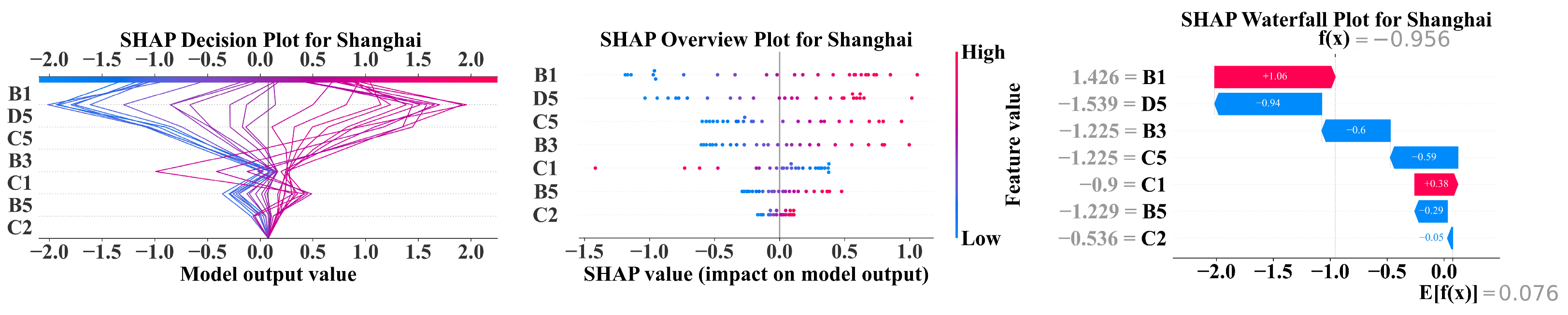
3.3. PPR for Driving Factor Selection

After addressing multicollinearity successfully, this paper further used PPR to select the key driving factors. The weights of the driving factors for each category of provinces are shown in Figure 6.

As shown in Figure 6, the driving factors for different categories of provinces exhibited significant differences after the PPR. Initially, this paper selected the driving factors with weights greater than 0.1 as the effective driving factors for each province. Then, the driving factors that were shared by more than 80% of the provinces within the same category were chosen as the representative driving factors for that category. The final effective driving factors for each category are shown in

Table 3. Effective driving factors for each category.

Category	Effective Driving Factors
Low-carbon potential provinces (LCPPs)	C2, B3, D2, A3, A1, C1, D6, C4, C6, C3, B5, B4
Economic growth hub provinces (EGHPs)	C1, B5, D5, D7, C6, C2, C3, D2, C4, D4, D6, A4, A1, A3
High-carbon-dependent provinces (HCDPs)	A4, B3, C1, C2, D6, B4, C6, A3, D7, E1, B1
Sustainable growth provinces (SGPs)	C1, A3, A4, B5, C6, C2, B3, C3, E1, D5, B4, D3, D2, C4, D6, A1
Low-carbon technology-driven provinces (LCTDPs)	C2, C1, B5, C5, D5, B1, B3

.

As shown in Table 3, LCPPs concentrated on optimizing energy structures and enhancing technological innovation to mitigate carbon emissions. These provinces aimed to increase the utilization of renewable energy sources, facilitated by external support mechanisms. EGHPs adeptly balanced economic growth with environmental stewardship by adjusting industrial structures and integrating technological innovations. HCDPs, which traditionally relied on conventional energy sources and exhibited high levels of carbon emissions, progressively shifted towards cleaner energy alternatives and improved energy efficiency through advanced technological upgrades. SGPs adopted comprehensive strategies that encompassed energy structure optimization, technological innovation, and supportive policy frameworks to achieve sustainable development. This approach effectively alleviated environmental pressures by promoting green technologies and renewable energy solutions. Meanwhile, LCTDPs prioritized the development and deployment of low-carbon technologies. Leveraging their advanced research facilities and innovative enterprises, these provinces drove technological advancements and offered critical technical support to facilitate similar transitions in other regions. In summary, both technological advancement and energy consumption patterns played pivotal roles in shaping the developmental trajectories of different provinces. Optimizing energy structures and upgrading technologies were essential for achieving sustainable development across all provinces.

3.4. GM-SVR Carbon Emission Prediction Model

3.4.1. Driving Factor Prediction

Considering the sample size of the dataset for each category of provinces was relatively small, this paper used the GM model to predict the values of key driving factors for each category of provinces in China from 2022 to 2032. Therefore, Hainan, Liaoning, Shandong, Heilongjiang, and Shanghai were selected for presentation from the LCPPs, EGHPs, HCDPs, SGPs, and LCTDPs categories, respectively. The results are shown in

Table 4. GM-predicted driving factors for the five categories of provinces.

Province	Factor	2027	2028	2029	2030	2031
Hainan (LCPPs)	C1	70,003.93	76,783.04	84,218.63	92,374.28	101,319.70
	C2	26,654.30	28,043.98	29,506.10	31,044.46	32,663.03
	D5	455.33	468.52	482.10	496.07	510.44
Liaoning (EGHPs)	C1	15,186,425.47	17,646,268.75	20,504,548.71	23,825,802.71	27,685,021.65
	C2	74,335.99	75,319.90	76,316.83	77,326.95	78,350.45
	D5	2371.90	2532.60	2704.17	2887.38	3082.99
Shandong (HCDPs)	C1	59,327,768.93	65,207,510.88	77,094,826.87	87,512,060.07	90,219,269.12
	C2	114,268.81	114,535.20	114,802.20	115,069.82	115,338.07
	B1	41.08	40.68	40.29	39.90	39.51
Heilongjiang (SGPs)	C1	8,159,351.428	9,517,661.358	11,102,092.92	12,950,289.21	15,106,159.89
	C2	21,797.98	21,228.48	20,673.87	20,133.75	19,607.74
	D5	483.43	485.75	488.08	490.42	492.77
Shanghai (LCTDPs)	C1	38,685,401.75	44,225,406.57	50,558,776.64	57,799,127.11	66,076,343.53
	C2	4075.18	4163.22	4253.17	4345.06	4438.93
	B1	24.31	23.68	23.07	22.47	21.89

.

For a comprehensive evaluation of the GM model’s predictive performance, this paper selected the small error probability P and the posterior variance ratio as the key indicators for measuring the accuracy of the grey model’s predictions. Generally speaking, when P exceeds 0.95 and C is below 0.35, the predictive accuracy of the grey model is considered excellent. Then, if P is greater than 0.8 and C is below 0.5, the model’s accuracy is deemed acceptable. Additionally, when P exceeds 0.7 and C is below 0.65, the model is considered barely acceptable. If neither of these conditions are met, the predictive accuracy of the model is regarded as poor. The proportions of grey model accuracy levels for each category are shown in Figure 7.

As shown in Figure 7, for more than 95% of the provinces across the five categories, the GM prediction accuracy level was at least barely acceptable or higher. Among these categories, 61% to 68% of the provinces exhibited good prediction accuracy, indicating that the grey model demonstrated reliable performance across all five categories.

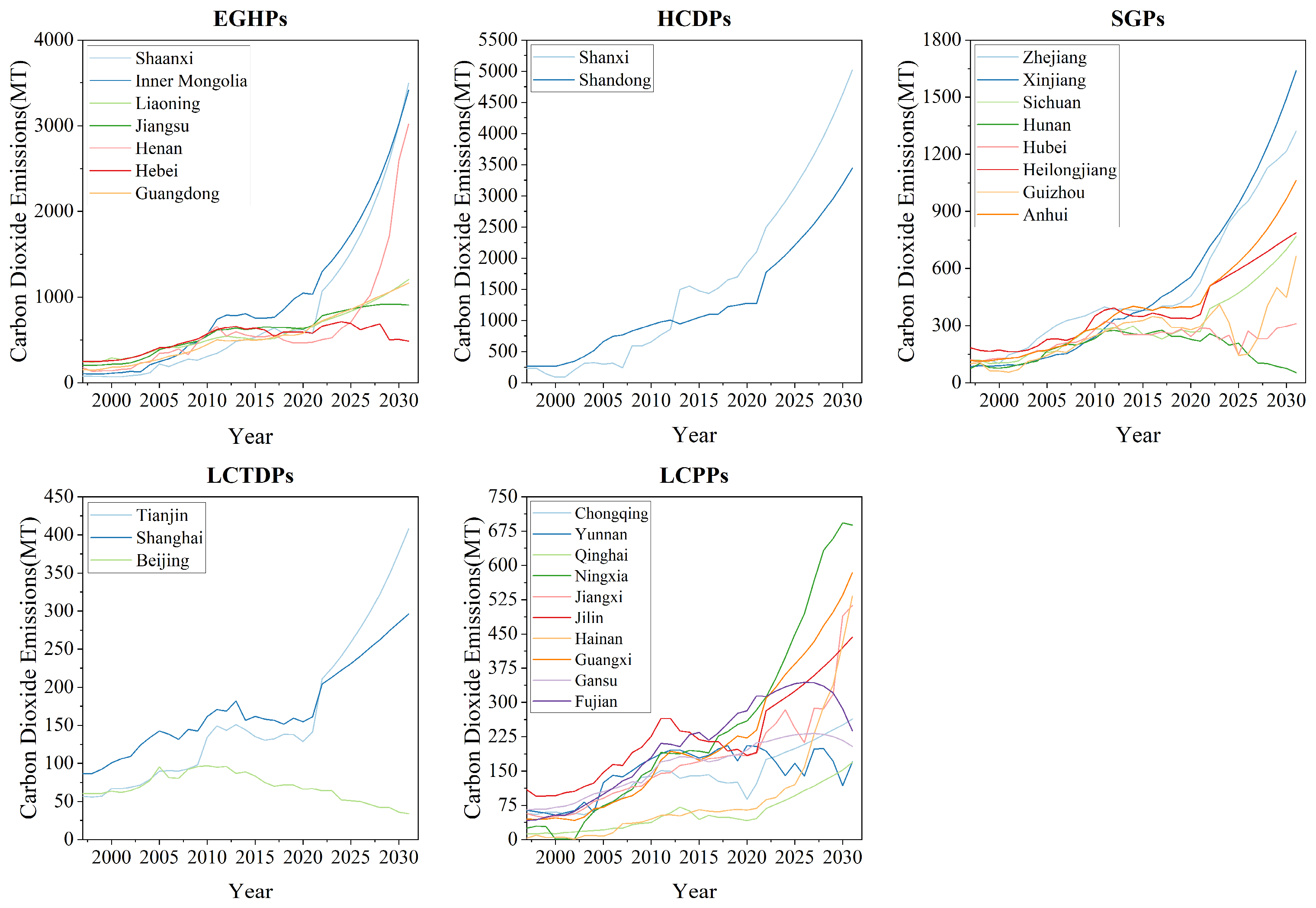
3.4.2. Carbon Emission Prediction

Based on the GM model to predict the driver values of various provinces from 2022 to 2032, this paper used the TPE algorithm to optimize the parameters of the SVR for predicting carbon emissions over the next decade. For data processing, 80% of the data from 1997 to 2022 were extracted as the training dataset, and the remaining 20% were extracted as the test dataset. The predicted carbon emission values for each category of provinces from 2022 to 2032 are shown in Figure 8.

As shown in Figure 8, EGHPs were projected to continue their significant increase, demonstrating a sustained and rapid growth trend. HCDPs, which were already at high levels, were expected to show a slow upward trend. Despite currently low emissions, SGPs were anticipated to experience moderate growth. In contrast, the carbon emissions of LCTDPs and LCPPs were expected to remain at lower levels with a relatively stable growth trend.

3.5. Comparative Analysis of Multiple Prediction Models

To evaluate the prediction performance of the GM-SVR model and compare it with other prediction models, this paper adopted three evaluation metrics: the average Root Mean Squared Error (RMSE), Mean Absolute Error (MAE), and the Coefficient of Determination (R²).

RMSE measures the average difference between the predicted values and the actual values. Its formula is expressed as Equation (21):

$$RMSE=\sqrt{{\displaystyle \frac{1}{n}}{\displaystyle \sum _{i=1}^n}{\left(y_i-{\widehat{y}}_i\right)}^2},$$

(21)

where $y_i$ represents the actual value, ${\widehat{y}}_i$ represents the predicted value, and n represents the sample size.

MAE measures the average absolute difference between the predicted and actual values. The formula is expressed as Equation (22):

$$MAE={\displaystyle \frac{1}{n}}{\displaystyle \sum _{i=1}^n}\left|y_i-{\widehat{y}}_i\right|,$$

(22)

where $y_i$ is the actual value, ${\widehat{y}}_i$ is the predicted value, and n is the sample size.

The Coefficient of Determination measures the proportion of variance in the dependent variable that is explained by the model. The value of R² ranges from 0 to 1, where a value closer to 1 indicates a better model fit. The formula is expressed as Equation (23):

$$R^2=1-{\displaystyle \frac{{\sum }_{i=1}^n{\left(y_i-{\widehat{y}}_i\right)}^2}{{\sum }_{i=1}^n{\left(y_i-{\overline{y}}_i\right)}^2}},$$

(23)

where $y_i$ denotes the actual value, ${\widehat{y}}_i$ denotes the predicted value, n denotes the sample size, and ${\overline{y}}_i$ denotes the mean of the actual values.

To ensure the robustness and generalization capability of the models, this paper employed 5-fold cross-validation for the GM-SVR model. The results of the 5-fold cross-validation are shown in

Table 5. 5-fold cross-validation results for SVR model.

Fold	RMSE	MAE	R2
1	0.158	0.150	0.952
2	0.165	0.154	0.957
3	0.160	0.152	0.954
4	0.159	0.153	0.956
5	0.164	0.156	0.955
Avg	0.161	0.153	0.955

.

As shown in Table 5, the SVR model demonstrated strong predictive performance and robustness across all five folds. What is more, RMSE, MAE, and R² scores indicate that the model is reliable.

With the model’s robustness confirmed via 5-fold cross-validation, this paper further compared the performance of multiple prediction models using the same evaluation metrics. The comparison of various models’ metrics is shown in

Table 6. Comparison of prediction methods.

Algorithm	RMSE	MAE	R2
GM	0.345	0.351	0.671
LSTM	0.315	0.342	0.678
SVR	0.315	0.234	0.684
X-GBOOST	0.475	0.443	0.618
Random Forest	0.272	0.254	0.765
GM-SVR	0.161	0.153	0.955

.

As shown in Table 6, the GM-SVR model exhibited a significantly higher R² compared to other models, indicating its superior performance in explaining data variability and fitting accuracy. Additionally, the GM-SVR model’s RMSE and MAE were lower than those of other models, reaching 0.161 and 0.153, respectively. This demonstrated that the GM-SVR model had a clear advantage in predicting the driving factors for each province from 2022 to 2032.

4. Discussion

4.1. Heterogeneity Analysis of Regional Carbon Emissions

Based on the results obtained from SHAP, this paper established a PEST-SWOT model to analyze the five regions. For the SHAP results, Hainan, Liaoning, Shandong, Heilongjiang, and Shanghai from LCPPs, EGHPs, HCDPs, SGPs, and LCTDPs were selected for visualization. The visualization results are shown in Figure 9, Figure 10, Figure 11, Figure 12 and Figure 13.

Figure 9 demonstrate that in LCPPs, coal and electricity consumption had a significant negative impact on carbon emissions, while per capita GDP and total regional GDP had positive effects. Railway passenger volume negatively affected carbon emissions, and urban population size showed mixed effects depending on the province. In EGHPs, coal and electricity consumption negatively impacted carbon emissions, while urban population size also had a negative effect. Market transaction volume and domestic patent applications positively influenced carbon emissions, with per capita GDP showing mixed effects across provinces. In HCDPs, urban population size, green coverage of built-up areas, and electricity consumption all had negative effects on carbon emissions, while per capita GDP and total GDP showed a larger negative impact. Additionally, the proportion of secondary industry in GDP had a positive effect. In SGPs, coal and electricity consumption affected carbon emissions negatively and per capita GDP and total GDP showed negative effects. What is more, urban population impacted carbon emissions negatively, while market transaction volume influenced it positively. In LCTDPs, per capita GDP and diesel consumption had large negative effects on carbon emissions, while the proportion of secondary industry in GDP had a positive impact. Additionally, market transaction volume positively influenced carbon emissions, while education funding and road passenger traffic had negative effects. Based on PEST-SWOT analysis, this paper analyzed regional heterogeneity from four perspectives: political, economic, social, and technological.

4.1.1. Political Factors

• LCPPs: The political will of the government to promote low-carbon policies and reduce carbon emissions plays a critical role in shaping regional carbon emission trends. For instance, policies focused on clean energy development and energy efficiency improvements to reduce coal and electricity consumption. Additionally, the government’s political stability and emphasis on environmental protection influence the control and reduction of high-carbon energy sources. Policies such as energy consumption caps, green tax incentives, and support for renewable energy projects could be crucial in decreasing the reliance on coal. Furthermore, government initiatives can influence factors such as railway passenger volume and urban population distribution by promoting public transportation and urban development in environmentally friendly ways;
• EGHPs: In this category, the government’s adoption of strict energy control policies directly influences carbon emissions. Specific policies include carbon tax regulations, energy consumption quotas, and incentives for energy efficiency improvements in industries. The government may also provide financial support and subsidies to foster technological innovation, particularly in clean technologies such as renewable energy, carbon capture, and energy storage solutions. Support for domestic patent applications in green technologies also contributes to reducing carbon emissions by promoting local innovation in low-carbon solutions. These regions might also focus on green infrastructure to manage urban growth and reduce emissions;
• HCDPs: Government policies aimed at green development are particularly significant in reducing carbon emissions in these high-carbon-dependent provinces. For instance, policies may involve phasing out coal plants, incentivizing renewable energy adoption, and promoting energy-efficient technologies. Political transparency and public participation in environmental decision making can enhance the effectiveness of these policies. Furthermore, local governance plays an important role in the implementation of environmental protection laws, such as stricter emission standards and environmental impact assessments for industrial projects. Policies supporting electricity consumption reduction and public education on energy conservation are likely to be emphasized in these regions;
• SGPs: Political decisions regarding energy consumption directly influence carbon emissions, especially in the management of coal and electricity use. Governments may adopt energy transition policies that focus on reducing the share of coal in energy production and increasing the use of renewable energy sources. In addition, the government might introduce green technology support policies, such as subsidies for electric vehicles, solar power projects, and carbon emission reduction targets. These measures are designed to reduce the carbon footprint of key industries, particularly in manufacturing and transportation sectors. By focusing on low-carbon technology adoption, these provinces can further their goals of reducing emissions;
• LCTDPs: Policy guidance is vital in promoting an increase in the share of the secondary industry while reducing diesel consumption. For example, tax incentives for green technologies, subsidies for electric transportation, and carbon credit systems can play a central role. Governments may also provide strong support for education, promoting green technologies through research funding and the development of training programs for low-carbon industries. Additionally, transportation policies focusing on public transit and electric vehicle infrastructure could contribute to overall carbon reduction efforts. Technology development policies might include research and development (R&D) grants for low-carbon innovation, ensuring that these provinces maintain a technological edge in reducing their carbon emissions.

4.1.2. Economic Factors

• LCPPs: Economic transformation and industrial upgrading impact carbon emissions significantly. Also, high GDP regions are often accompanied by higher energy consumption and carbon emissions, especially in areas relying on traditional high-carbon energy. However, economic efficiency helps reduce carbon emission pressure;
• EGHPs: Economic openness, market transaction volume, and patent application volume are key economic factors driving green innovation and low-carbon technology application. Also, accelerated economic development can increase energy demand, leading to higher carbon emissions. However, the development of a green economy and environmental investments can mitigate this growth;
• HCDPs: The speed of economic growth is highly correlated with carbon emissions. Excessive reliance on heavy industry or high-carbon industries will increase emissions, while optimizing economic structure can help reduce emissions. In addition, the increase in per capita GDP has a noticeable effect on driving carbon emissions;
• SGPs: In this category, the proportion of coal and electricity consumption is directly linked to the stage of economic development. Economic development often leads to increased energy demand, resulting in higher carbon emissions. However, restructuring to rely on low-carbon technologies and clean energy may help reduce emissions;
• LCTDPs: The proportion of the secondary industry in the economic structure and energy consumption patterns impact carbon emissions. However, economic growth, especially industrialization, will increase carbon emissions unless there is a transition to clean energy technologies.

4.1.3. Social Factors

• LCPPs: Urban population density and demographic changes impact energy consumption and carbon emissions significantly. During urbanization, energy demand tends to rise, leading to higher carbon emissions. However, increased social awareness of environmental protection and energy conservation can alleviate this impact;
• EGHPs: Social culture, education levels, and environmental awareness affect carbon emissions significantly. As society deepens its understanding of the low-carbon economy, residents’ low-carbon lifestyles will contribute to reducing emissions. Meanwhile, social behavior and policy support will promote the application of low-carbon technologies;
• HCDPs: Urban population and urbanization have a particularly strong effect on carbon emissions. What is more, increased population density may lead to more energy demand, with transportation, buildings, and industries raising emissions. Additionally, social support and participation in environmental policies will influence the application of low-carbon technologies and emission reduction;
• SGPs: The public’s acceptance of low-carbon lifestyles is closely related to carbon emissions. As environmental policies and green technologies become more popular, social support for reducing energy consumption and carbon emissions gradually increases, facilitating a society-wide low-carbon transition;
• LCTDPs: Social structure, population mobility, and urbanization are closely related to carbon emissions. As per capita GDP and social welfare increase, energy demand typically rises, which may lead to higher carbon emissions.

4.1.4. Technological Factors

• LCPPs: Technological progress affects energy consumption patterns and carbon emissions directly, especially breakthroughs in clean energy and energy-saving technologies. Therefore, the adoption of advanced green technologies can significantly reduce coal and electricity consumption, thereby lowering emissions;
• EGHPs: Technological innovation, especially in the areas of energy savings, emission reduction, and low-carbon technologies, plays a crucial role in reducing carbon emissions. As market transaction volumes and patent applications increase, the research and application of low-carbon technologies will help control emissions;
• HCDPs: Technological advancements can improve energy efficiency effectively, especially in electricity consumption and building sectors. Additionally, the widespread use of green technologies in energy-saving, environmental protection, and clean production reduces carbon emissions directly;
• SGPs: Technological advancements are crucial in reducing carbon emissions. Emerging technologies will drive the green transformation of the energy structure to reduce dependence on high-carbon energy sources like coal and electricity, including high-efficiency energy, clean energy, and low-carbon production processes;
• LCTDPs: Innovations in green technologies for industrial production and energy consumption affect carbon emissions directly. Thanks to green technologies, the reduction in diesel consumption and improved energy efficiency in the secondary industry will reduce carbon emissions. Advances in sustainable energy will drive the transition to a low-carbon economy.

4.1.5. SWOT-Analysis

1.

LCPPs

(1)

Strengths

• Government Policy Support: policies such as clean energy development and energy efficiency improvements help reduce coal and electricity consumption;
• Political Stability: strong policy stability is conducive to achieving long-term low-carbon goals;
• High Public Awareness of Environmental Protection: with the improvement of environmental awareness, public support for low-carbon living and energy conservation helps in the implementation of policies.

(2)

Weaknesses

• High Dependency on Coal: despite government green energy policies, certain regions remain heavily dependent on coal, with a slow transition process;
• Economic Transition Challenges: some low-carbon potential provinces still lag in industrial restructuring and technological innovation, leading to high energy demand for economic growth.

(3)

Opportunities

• National-Level Policy Support: policies such as green tax incentives and renewable energy project support help accelerate the application of green technologies in these regions;
• Emerging Green Technologies: technological innovations can effectively reduce dependence on coal and electricity, driving regional low-carbon transitions.

(4)

Threats

• External Economic Competitive Pressure: during the low-carbon transition, there may be competitive pressure from other provinces or countries in the development of green technologies;
• Inconsistent Policy Implementation: local governments may have differences in implementing green policies, leading to uneven transition progress.

2.

EGHPs

(1)

Strengths

• Government Promotion of Green Technologies: the government supports the popularization of low-carbon technologies through policies such as green infrastructure construction and innovation subsidies;
• Strong Market Activity and Patent Applications: these factors promote local innovation and the application of green technologies.

(2)

Weaknesses

• Increased Energy Demand from Economic Growth: rapid economic development leads to higher energy consumption and carbon emissions, especially in high-carbon industries that rely on traditional energy sources.

(3)

Opportunities

• Green Economic Investment: investment and support for green technologies, both domestic and international, provide opportunities for these regions to develop low-carbon industries;
• Renewable Energy: government support for clean energy technologies can accelerate the pace of green transition.

(4)

Threats

• Structural Dependence on High-Carbon Industries: despite green policies, reliance on traditional high-carbon industries may limit the effectiveness of the low-carbon transition;
• Inconsistency in Local Government Policy Implementation: differences in local government execution of low-carbon policies may affect the overall emission reduction results.

3.

HCDPs

(1)

Strengths

• Government Policies Shifting Toward Low Carbon: policies aimed at promoting green technologies and improving energy efficiency are gradually being implemented;
• Significant Potential for Technological Advancements: particularly in energy efficiency and building energy conservation, there is considerable room for improvement.

(2)

Weaknesses

• Reliance on Heavy Industry or High-Carbon Industries: the transformation pressure is substantial due to the reliance on these industries;
• High Energy Consumption in Densely Populated Areas: this leads to higher carbon emissions.

(3)

Opportunities

• National Policy Support and Local Government Green Development Projects: these can help accelerate the low-carbon transition;
• Widespread Application of Green Technologies: clean energy and energy-saving technologies can effectively reduce carbon emissions.

(4)

Threats

• Competition from High-Carbon Industries: the difficulty in reforming traditional industries may increase the pressure on low-carbon transition;
• Policy Implementation Effectiveness: local government execution of policies may not meet expectations, especially if local governments lack sufficient enforcement.

4.

SGPs

(1)

Strengths

• Active Government Policies on Energy Consumption Management and Reducing Coal Use: the government has taken proactive steps in managing energy consumption and reducing coal use;
• Market Transactions and Technological Innovation Support: these support the promotion of low-carbon technologies, contributing to carbon emissions control.

(2)

Weaknesses

• Dependency on High-Carbon Energy in Industrial Structure: economic growth could lead to increased energy demand and carbon emissions;
• Low Public Awareness of Low-Carbon Living: this hinders the widespread adoption of low-carbon technologies.

(3)

Opportunities

• Energy Structure Transformation: government efforts to promote low-carbon energy and technologies enhance the green transformation of industrial structures;
• Low-Carbon Technology Support Policies: subsidies and green technology incentives help accelerate industrial transformation.

(4)

Threats

• Over-reliance on Coal and Traditional Energy: this could obstruct the low-carbon transition process;
• External Market and Policy Changes: changes in the global green economy and intense competition could heighten transition pressure.

5.

LCTDPs

(1)

Strengths

• Strong Government Green Policies: these policies focus on energy structure adjustments and the application of low-carbon technologies;
• Market Activity and Technological Innovation: these factors help promote low-carbon technologies and the development of local green industries.

(2)

Weaknesses

• Challenges in Industrial Restructuring: difficulties remain in transforming high-carbon industries, leading to pressure in transitioning the economy;
• Limited Green Technology Diffusion: the popularization of green technologies is still constrained by technology maturity and insufficient funding.

(3)

Opportunities

• Technological Innovation and Increased Market Transactions: these push the application of low-carbon technologies, especially in electric transportation and clean energy;
• National Policy Support: national-level policies provide more green investment opportunities for these regions.

(4)

Threats

• Rapid Technological Iteration: the fast pace of green technology advancement may leave some regions behind in terms of technology updates;
• Short-Term Goals of Local Governments and Markets: inconsistent implementation of low-carbon policies may affect overall results due to the focus on short-term objectives.

4.2. Future Development Suggestions

4.2.1. LCPPs

Low-carbon potential regions need to intensify research and promotion of low-carbon technologies and drive energy structural transformation through policy support and innovation. The focus should be on improving energy efficiency, promoting clean energy, developing green transportation, and applying energy-saving technologies. Also, the government should enhance environmental protection regulations, raise public awareness, and reduce coal and electricity consumption. Investments in green technologies should be accelerated, especially during urbanization, with a focus on green building and low-carbon transport systems, such as smart grids and renewable energy.

4.2.2. EGHPs

Economic growth regions should lead with a green economy, promoting the gradual substitution of high-carbon energy. In addition, increasing economic openness and market transaction volume will facilitate green innovation and the adoption of low-carbon technologies to reduce carbon emissions further. Also, optimizing industrial structure and reducing dependence on high-carbon energy will promote green industrial development. From the government’s perspective, they should strengthen green investment and support low-carbon technology research and development through policy incentives.

4.2.3. HCDPs

High-carbon resource-dependent regions should prioritize industrial restructuring, reducing reliance on heavy industry and high-carbon industries and promoting green economic transformation. The focus should be on improving clean energy and environmental technology applications, improving energy efficiency, and reducing electricity consumption and carbon emissions. For the government, they should intensify support for green technologies, especially in construction and transportation, and promote green buildings and green transportation.

4.2.4. SGPs

For sustainable growth regions, green technology leadership should be strengthened to achieve a win–win outcome between the economy and the environment. Additionally, increased policy support and financial investment in green industries should be encouraged, especially in clean energy, low-carbon manufacturing, and green buildings. At the same time, enhancing technological innovation capabilities through international cooperation will lead to breakthroughs in these areas, especially in smart grids, energy storage, and carbon capture. Carbon market mechanisms should be enhanced to promote carbon pricing and trading, motivating enterprises and society to reduce emissions.

4.2.5. LCTDPs

Especially in the field of industrial production and energy consumption, the future development of low-carbon technology-led regions should continue to strengthen green technology innovation and promote the wide application of clean energy. Meanwhile, the government should support the green development of the secondary industry. Also, the government should encourage the use of low-carbon production processes and energy-saving technologies to reduce diesel consumption and carbon emissions. Coordinated development of education and technology policies will accelerate the low-carbon transition, while technological progress will improve industrial energy efficiency and lower carbon emissions.

5. Conclusions

In order to address the global challenge of climate change effectively, China, as the world’s second-largest economy, plays a crucial role in this grand process. Therefore, this paper employed the adaptive k-means++ clustering algorithm to classify provinces across the country into five categories: LCPPs, EGHPs, HCDPs, SGPs, and LCTDPs. This classification provided a solid foundation for the subsequent selection of driving factors and the construction of predictive models. For the five classified categories of provinces, this paper used the Spearman correlation analysis method to reveal the presence of multicollinearity among driving factors within each category and employed Lasso regression to resolve this issue. What is more, the PPR algorithm was used to further select the key driving factors. Subsequently, the grey prediction model was applied to predict the driving factors for carbon emissions from 2022 to 2032 for each category of province. Based on the GM model’s predictions for driving factors, an SVR model optimized using the TPE algorithm was used to forecast carbon emissions from 2022 to 2032. Compared with other forecasting algorithms, this paper showed that the GM-SVR model exhibited significant superiority and prediction accuracy.

Finally, by combining SHAP and PEST-SWOT analyses, this paper provides an in-depth examination of the intricate relationships between carbon emission reductions and four critical dimensions: political will, economic structure, social culture, and technological progress. Specifically, for the LCPPs region, efforts should focus on enhancing low-carbon technology research and promotion, with the government strengthening investment in environmental policies and green technologies. For the EGHPs region, promoting a green economic transformation, optimizing the industrial structure, reducing reliance on high-carbon energy, and supporting the application of low-carbon technologies through policy incentives are crucial. For the HCDPs region, prioritizing industrial structure optimization and increasing the use of clean energy should be the focus. For the SGPs region, attention should be paid to green technological innovation, promoting low-carbon economic transformation, and fostering international cooperation and carbon market mechanisms to advance low-carbon development. For the LCTDPs region, continued promotion of green technological innovation should aim to further reduce carbon emissions guided by policies and green investment. Overall, to achieve the goal of effective control of carbon emissions and sustainable development, all kinds of regions should adopt feasible policies according to their own characteristics.

Despite the achievements of this paper, some limitations remain. Initially, model assumptions may fail to fully reflect the complexity and dynamic changes in real situations. Next, more detailed zoning and personalization strategies may still be needed in practice. Future studies could consider improving data collection mechanisms, improving the accuracy and completeness of the data, and developing models with more dynamic adjustment capabilities to respond to changes in economic structure and technological progress in real time.

References

1. Fang, J.; Zhu, J.; Wang, S.; Yue, C.; Shen, H. Global warming, human-induced carbon emissions, and their uncertainties. Sci. China Earth Sci. 2011, 54, 1458–1468. [Google Scholar] [CrossRef]
2. Sun, W.; Huang, C. Predictions of carbon emission intensity based on factor analysis and an improved extreme learning machine from the perspective of carbon emission efficiency. J. Clean. Prod. 2022, 338, 130414. [Google Scholar] [CrossRef]
3. Fang, K.; Tang, Y.; Zhang, Q.; Song, J.; Wen, Q.; Sun, H.; Ji, C.; Xu, A. Will China peak its energy-related carbon emissions by 2030? Lessons from 30 Chinese provinces. Appl. Energy 2019, 255, 113852. [Google Scholar] [CrossRef]
4. Lin, C.; Li, X. Carbon peak prediction and emission reduction pathways exploration for provincial residential buildings: Evidence from Fujian Province. Sustain. Cities Soc. 2024, 102, 105239. [Google Scholar] [CrossRef]
5. Chen, M.; Zhang, J.; Xu, Z.; Hu, X.; Hu, D.; Yang, G. Does the setting of local government economic growth targets promote or hinder urban carbon emission performance? Evidence from China. Environ. Sci. Pollut. Res. 2023, 30, 117404–117434. [Google Scholar] [CrossRef]
6. Zheng, Y.; Tang, J.; Huang, F. The impact of industrial structure adjustment on the spatial industrial linkage of carbon emission: From the perspective of climate change mitigation. J. Environ. Manag. 2023, 345, 118620. [Google Scholar] [CrossRef]
7. Zhao, J.; Ji, G.; Yue, Y.; Lai, Z.; Chen, Y.; Yang, D.; Yang, X.; Wang, Z. Spatio-temporal dynamics of urban residential CO2 emissions and their driving forces in China using the integrated two nighttime light datasets. Appl. Energy 2019, 235, 612–624. [Google Scholar] [CrossRef]
8. Caiado, R.G.G.; Filho, W.L.; Quelhas, O.L.G.; Nascimento, D.L.M.; Ávila, L.V. A literature-based review on potentials and constraints in the implementation of the sustainable development goals. J. Clean. Prod. 2018, 198, 1276–1288. [Google Scholar] [CrossRef]
9. Wang, Y.; Dong, L. Research on carbon peak prediction of various prefecture-level cities in Jiangsu Province based on factors influencing carbon emissions. Sustainability 2024, 16, 7105. [Google Scholar] [CrossRef]
10. Wei, Z.; Wei, K.; Liu, J.; Zhou, Y. The relationship between agricultural and animal husbandry economic development and carbon emissions in Henan Province, the analysis of factors affecting carbon emissions, and carbon emissions prediction. Mar. Pollut. Bull. 2023, 193, 115134. [Google Scholar] [CrossRef]
11. Zhao, J.; Kou, L.; Wang, H.; He, X.; Xiong, Z.; Liu, C.; Cui, H. Carbon emission prediction model and analysis in the Yellow River Basin based on a machine learning method. Sustainability 2022, 14, 6153. [Google Scholar] [CrossRef]
12. Dai, D.; Zhou, B.; Zhao, S.; Lu, K.; Liu, Y. Research on industrial carbon emission prediction and resistance analysis based on CEI-EGM-RM method: A case study of Bengbu. Sci. Rep. 2023, 13, 14528. [Google Scholar] [CrossRef] [PubMed]
13. Yan, R.; Chen, M.; Xiang, X.; Feng, W.; Ma, M. Heterogeneity or illusion? Track the carbon Kuznets curve of global residential building operations. Appl. Energy 2023, 347, 121441. [Google Scholar] [CrossRef]
14. Zou, C.; Ma, M.; Zhou, N.; Feng, W.; You, K.; Zhang, S. Toward carbon free by 2060: A decarbonization roadmap of operational residential buildings in China. Energy 2023, 277, 127689. [Google Scholar] [CrossRef]
15. Zhang, S.; Wang, M.; Zhu, H.; Jiang, H.; Liu, J. Impact factors and peaking simulation of carbon emissions in the building sector in Shandong Province. J. Build Eng. 2024, 87, 109141. [Google Scholar] [CrossRef]
16. Yang, J.; Cai, W.; Ma, M.; Li, L.; Liu, C.; Ma, X.; Li, L.; Chen, X. Driving forces of China’s CO2 emissions from energy consumption based on Kaya-LMDI methods. Sci. Total Environ. 2020, 711, 134569. [Google Scholar] [CrossRef]
17. Zhu, B.; Ye, S.; Han, D.; Wang, P.; He, K.; Wei, Y.; Xie, R. A multiscale analysis for carbon price drivers. Energy Econ. 2019, 78, 202–216. [Google Scholar] [CrossRef]
18. Yu, Y.; Xu, W. Impact of FDI and R&D on China’s industrial CO2 emissions reduction and trend prediction. Atmos. Pollut. Res. 2019, 10, 1627–1635. [Google Scholar]
19. Sapnken, F.E.; Hong, K.R.; Noume, H.C.; Tamba, J.G. A grey prediction model optimized by meta-heuristic algorithms and its application in forecasting carbon emissions from road fuel combustion. Energy 2024, 302, 131922. [Google Scholar] [CrossRef]
20. Zhong, W.; Zhai, D.; Xu, W.; Gong, W.; Yan, C.; Zhang, Y.; Qi, L. Accurate and efficient daily carbon emission forecasting based on improved ARIMA. Appl. Energy 2024, 376, 12432. [Google Scholar] [CrossRef]
21. Ye, L.; Du, P.; Wang, S. Industrial carbon emission forecasting considering external factors based on linear and machine learning models. J. Clean. Prod. 2024, 434, 140010. [Google Scholar] [CrossRef]
22. Luo, C.; Gao, Y.; Jiang, Y.; Zhao, C.; Ge, H. Predictive modeling of carbon emissions in Jiangsu Province’s construction industry: An MEA-BP approach. J. Build Eng. 2024, 86, 108903. [Google Scholar] [CrossRef]
23. Jiang, X. Prediction method of carbon emissions of intelligent buildings based on secondary decomposition BAS-LSTM. Clean. Technol. Environ. Policy 2024. [Google Scholar] [CrossRef]
24. Niu, D.; Wang, K.; Wu, J.; Sun, L.; Liang, Y.; Xu, X.; Yang, X. Can China achieve its 2030 carbon emissions commitment? Scenario analysis based on an improved general regression neural network. J. Clean. Prod. 2020, 243, 118558. [Google Scholar] [CrossRef]
25. Sun, W.; Zhang, J. Analysis influence factors and forecast energy-related CO2 emissions: Evidence from Hebei. Environ. Monit. Assess 2020, 192, 665. [Google Scholar] [CrossRef]
26. Yao, Y.; Sun, Z.; Li, L.; Cheng, T.; Chen, D.; Zhou, G.; Liu, C.; Kou, S.; Chen, Z.; Guan, Q. CarbonVCA: A cadastral parcel-scale carbon emission forecasting framework for peak carbon emissions. Cities 2023, 138, 104354. [Google Scholar] [CrossRef]
27. Hou, Y.; Wang, Q.; Tan, T. Prediction of carbon dioxide emissions in China using shallow learning with cross validation. Energies 2022, 15, 8642. [Google Scholar] [CrossRef]
28. Green, F.; Stern, N. China’s changing economy: Implications for its carbon dioxide emissions. Clim. Policy 2016, 17, 423–442. [Google Scholar] [CrossRef]
29. Wang, A.; Hu, S.; Lin, B. Emission abatement cost in China with consideration of technological heterogeneity. Appl. Energy 2021, 290, 116748. [Google Scholar] [CrossRef]
30. Wang, Q.; Li, L. The effects of population aging, life expectancy, unemployment rate, population density, per capita GDP, urbanization on per capita carbon emissions. Sustain. Prod. Consum. 2021, 28, 760–774. [Google Scholar] [CrossRef]
31. Wang, Y.; Niu, Y.; Li, M.; Yu, Q.; Chen, W. Spatial structure and carbon emission of urban agglomerations: Spatiotemporal characteristics and driving forces. Sustain. Cities Soc. 2021, 78, 103600. [Google Scholar] [CrossRef]
32. Zhou, J.; Hu, T.; Wei, Z.; Ji, D. Evaluation of high-quality development level of regional economy and exploration of index obstacle degree: A case study of Henan Province. J. Knowl. Econ. 2024, 129, 107994. [Google Scholar] [CrossRef]
33. Li, X.; Zhang, X. A comparative study of statistical and machine learning models on carbon dioxide emissions prediction of China. Environ. Sci. Pollut. Res. 2023, 30, 117485–117502. [Google Scholar] [CrossRef] [PubMed]
34. Baldassi, C. Recombinator-k-means: An evolutionary algorithm that exploits k-means++ for recombination. IEEE Trans. Evol. Comput. 2022, 26, 991–1003. [Google Scholar] [CrossRef]
35. Geng, X.; Mu, Y.; Mao, S.; Ye, J.; Zhu, L. An improved k-means algorithm based on fuzzy metrics. IEEE Access 2020, 8, 217416–217424. [Google Scholar] [CrossRef]
36. McNeish, D.M. Using Lasso for predictor selection and to assuage overfitting: A method long overlooked in behavioral sciences. Multivariate Behav. Res. 2015, 50, 471–484. [Google Scholar] [CrossRef]
37. Gao, C.; Hu, Z.; Xiong, Z.; Su, Q. Grey prediction evolution algorithm based on accelerated even grey model. IEEE Access 2020, 8, 107941–107957. [Google Scholar] [CrossRef]
38. Wu, J.; Chen, X.; Zhang, H.; Xiong, L.; Lei, H.; Deng, S. Hyperparameter optimization for machine learning models based on Bayesian optimization. J. Electron. Sci. Technol. 2019, 17, 26–40. [Google Scholar]
39. Raghavendra, S.N.; Deka, P.C. Support vector machine applications in the field of hydrology: A review. Appl. Soft. Comput. 2014, 19, 372–386. [Google Scholar] [CrossRef]
40. Shan, Y.; Guan, D.; Zheng, H.; Ou, J.; Li, Y.; Meng, J.; Mi, J.; Zhu, L.; Zhang, Q. China CO2 emission accounts 1997–2015. Sci. Data 2018, 5, 170201. [Google Scholar] [CrossRef]
41. Shan, Y.; Huang, Q.; Guan, D.; Hubacek, K. China CO2 emission accounts 2016–2017. Sci. Data 2020, 7, 54. [Google Scholar] [CrossRef] [PubMed]
42. Shan, Y.; Liu, J.; Liu, Z.; Xu, X.; Shao, S.; Wang, P.; Guan, D. New provincial CO2 emission inventories in China based on apparent energy consumption data and updated emission factors. Appl. Energy 2016, 184, 742–750. [Google Scholar] [CrossRef]
43. Guan, Y.; Shan, Y.; Huang, Q.; Chen, H.; Wang, D.; Hubacek, K. Assessment to China’s recent emission pattern shifts. Earths Future 2021, 9, 11. [Google Scholar] [CrossRef]
44. Xu, J.; Guan, Y.; Oldfield, J.; Guan, D.; Shan, Y. China carbon emission accounts 2020–2021. Appl. Energy 2024, 360, 122837. [Google Scholar] [CrossRef]
45. Wang, A.; Hu, S.; Lin, B. Can environmental regulation solve pollution problems? Theoretical model and empirical research based on the skill premium. Energy Econ. 2020, 94, 105068. [Google Scholar] [CrossRef]
46. Andrée, B.P.J.; Chamorro, A.; Spencer, P.; Koomen, E.; Dogo, H. Revisiting the relation between economic growth and the environment; a global assessment of deforestation, pollution and carbon emission. Renew. Sustain. Energy Rev. 2019, 114, 109221. [Google Scholar] [CrossRef]
47. Yang, W.; Feng, L.; Wang, Z.; Fan, X. Carbon emissions and national sustainable development goals coupling coordination degree study from a global perspective: Characteristics, heterogeneity, and spatial effects. Sustainability 2023, 15, 9070. [Google Scholar] [CrossRef]
Figure 1. Algorithm structure diagram.
Sustainability 17 01786 g001
Figure 2. Province classification map.
Sustainability 17 01786 g002
Figure 3. Spatial distribution maps of the four classification variables. (a) Shows the CO2 emissions of each province; (b) shows the proportion of industrial development in each province; (c) shows the economic development of each province; (d) shows the market transaction volume of technological innovation in each province.
Sustainability 17 01786 g003
Figure 4. Silhouette coefficient plot for k-means++ clustering.
Sustainability 17 01786 g004
Figure 5. Correlation analysis heatmap for selected provinces.
Sustainability 17 01786 g005
Figure 6. Factor weights of carbon emission PPR for different categories. Note: The larger the circle and the darker the color, the stronger the correlation.
Sustainability 17 01786 g006
Figure 7. Pie chart of the grey model accuracy levels for the five categories of provinces.
Sustainability 17 01786 g007
Figure 8. Line chart of future 10-year carbon emissions for each category of provinces.
Sustainability 17 01786 g008
Figure 9. SHAP value visualization for LCPPs.
Sustainability 17 01786 g009
Figure 10. SHAP value visualization for EGHPs.
Sustainability 17 01786 g010
Figure 11. SHAP value visualization for HCDPs.
Sustainability 17 01786 g011
Figure 12. SHAP value visualization for SGPs.
Sustainability 17 01786 g012
Figure 13. SHAP value visualization for LCTDPs.
Sustainability 17 01786 g013