

Performance Prediction of a Water-Cooled Centrifugal Chiller in Standard Temperature Conditions Using In-Situ Measurement Data


Abstract
1. Introduction
1.1. Background and Objectives
1.2. Limitations of Previous Studies
1.3. Research Objectives and Scope
1.4. Key Contributions of This Study
2. Theoretical Considerations
2.1. Refrigeration Theory
2.1.1. COP of Chillers
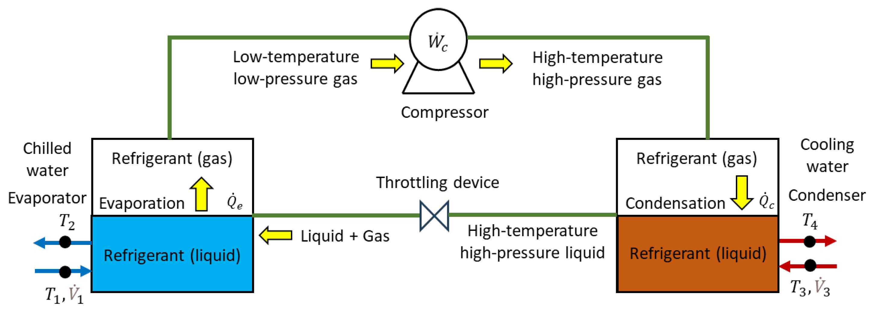
2.1.2. Thermodynamic Characteristics of Chillers
2.1.3. Energy Balance Error
2.2. Analysis Methods
- Analysis Based on Actual Operating Data: PLR is a commonly used metric for evaluating chiller performance under partial load conditions; however, it is defined under specific design conditions and may differ from real-time operating data [29]. This study focuses on analyzing chiller performance based on actual operating data, where the relationship between , , and COP is directly examined as a more practical approach.
- Challenges in Measuring and Calculating PLR: Incorporating PLR requires accurate measurement of the chiller’s rated cooling capacity and actual load, which is often subject to measurement errors and uncertainties in real-world conditions [30]. For instance, when building loads fluctuate significantly, PLR values may become inconsistent or inaccurate, reducing the reliability of the model. Therefore, this study prioritizes directly measurable variables (, , and COP) to enhance data reliability and model applicability.
- Generalization and Simplification of the Model: Previous studies that included PLR were often optimized under specific design conditions, which may limit their generalization across various operating environments [31]. By excluding PLR and instead utilizing more fundamental thermodynamic variables ( and ) in regression analysis, this study aims to develop a more universally applicable chiller performance prediction model that does not rely on specific load conditions.
- Thermodynamics-Based Approach: This study investigates the impact of and on COP through a thermodynamic perspective, aligning with established research that identifies evaporator and condenser temperature variations as key determinants of chiller performance [32]. In contrast, PLR primarily serves as an auxiliary metric representing load variation rather than a direct determinant of COP. Therefore, it was excluded from the regression model.
- Validation Through Data Analysis: The regression model developed using and as independent variables demonstrated strong predictive performance, with a high coefficient of determination ( > 0.8) and a low coefficient of variation of root mean square error (CVRMSE < 5%), indicating that chiller performance can be effectively modeled without incorporating PLR. Additionally, previous studies have proposed various approaches for evaluating chiller performance without using PLR [33].
Thermo-Regulated Residual Refinement Regression Model (TRRM)
2.3. Comparative Analysis Method
2.3.1. Simple Linear Regression Model (SL Model)
2.3.2. Bi-Quadratic Regression Model (BQ Model)
2.3.3. Multivariate Polynomial Regression Model (MP Model)
2.4. Review and Implications of Previous Studies
- Utilization of physics-based principles: Unlike purely data-driven models, TRRM incorporates thermodynamic residual adjustments to ensure compliance with the first law of thermodynamics, improving model reliability and reducing unrealistic predictions.
- Refinement of data-driven methodology: TRRM employs an iterative residual refinement process, systematically filtering out outliers caused by sensor noise, abnormal operating conditions, and measurement inaccuracies, which are common challenges in conventional regression-based models.
- Balancing accuracy and practicality: By limiting input variables to and while iteratively refining the dataset, TRRM achieves high predictive accuracy without requiring excessive data or complex parameter calibration, making it suitable for real-world applications.
2.4.1. Physics-Based Models
2.4.2. Data-Driven Models
2.4.3. Hybrid Approaches
2.5. Improvements of This Study
- Refines raw data by filtering out sensor noise and anomalies through a residual refinement process.
- Ensures thermodynamic consistency by applying energy balance constraints derived from the first law of thermodynamics.
- Improves generalization by training the model on carefully selected, high-quality data that represents diverse operating conditions, reducing dependency on case-specific parameters.
3. Research Methods
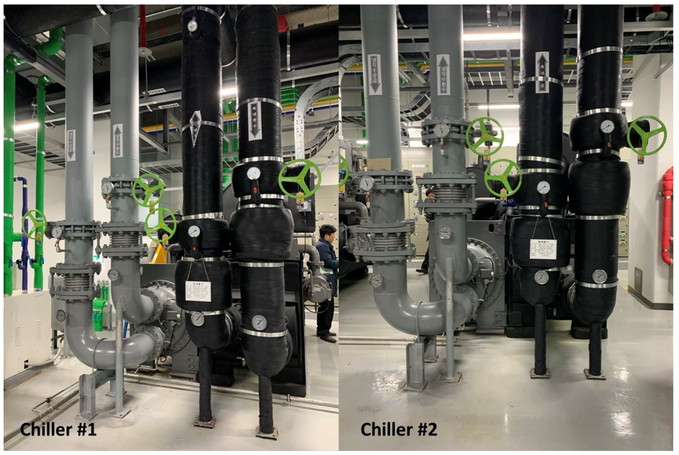
3.1. Measurement Target
- Ice-making operation: This process involves freezing the capsule-type media in the thermal storage tank, with the chiller operating at an average design temperature of −4.5 °C. Ice is primarily stored during late-night hours, and the system halts after 10 h of operation or upon reaching 100% storage capacity;
- Thermal storage-only operation: The chiller is not operated, and cooling loads are handled solely by the thermal storage tank. This mode is mainly used during transitional seasons or nighttime when cooling loads are minimal;
- Parallel operation of chiller and thermal storage tank: To manage peak cooling loads, the chiller operates in conjunction with the ice thermal storage tank, with the chiller running at normal operating temperatures;
- Chiller-only operation: The chiller independently handles cooling loads without utilizing the thermal storage tank. This mode is used in cases of thermal storage tank malfunction or after complete discharge of the stored ice.
3.2. Data Measurement
3.2.1. Data Measurement Method
3.2.2. Uncertainty Analysis
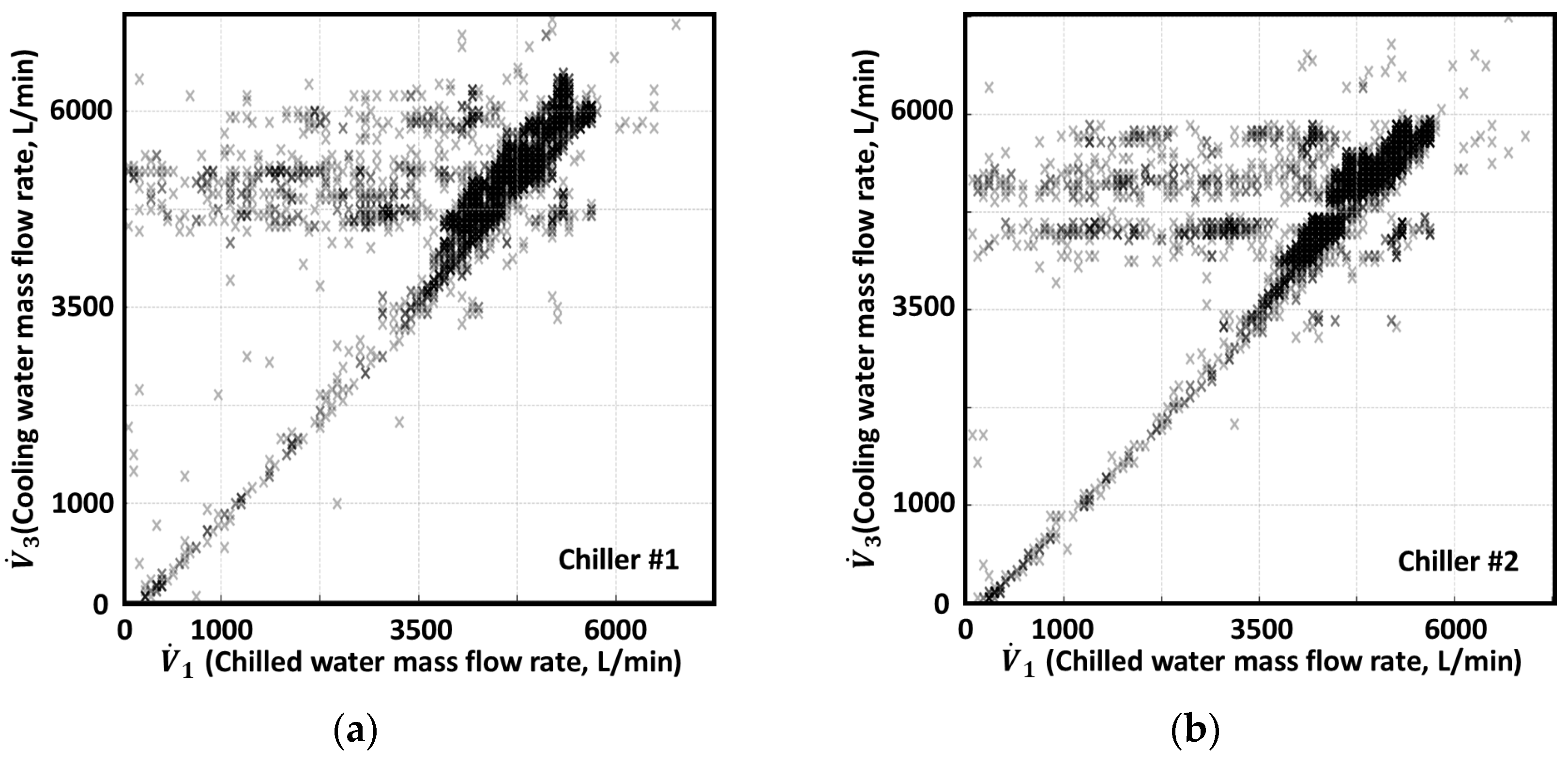
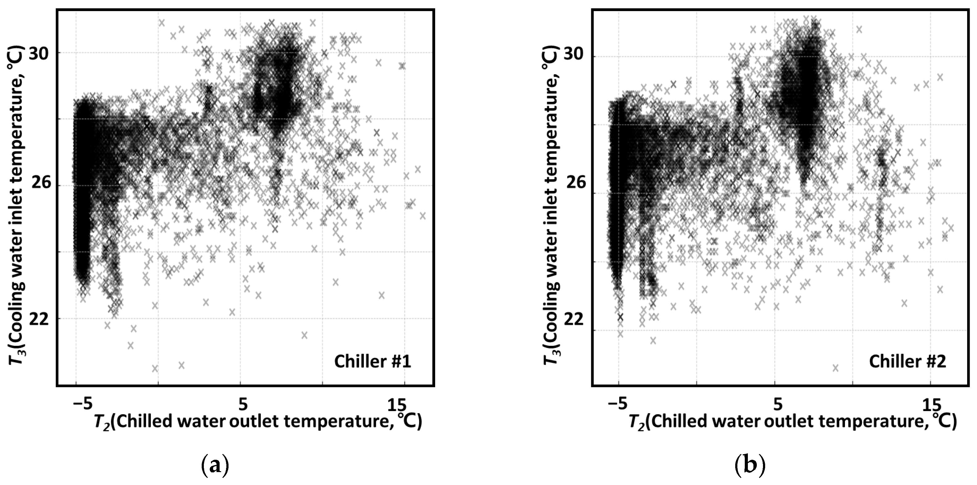
3.2.3. Flow Rate and Temperature Data Collection Results
- Difference in heat exchange processesIn chiller systems, heat exchange occurs in both the evaporator and the condenser. Chilled water (brine) absorbs heat in the evaporator and cools down, while cooling water absorbs heat in the condenser and facilitates refrigerant condensation. The cooling water must remove the total heat rejection , which is greater than the evaporator cooling load . This phenomenon is dictated by the first law of thermodynamics, expressed as . Since the compressor work is always positive, the total heat rejected must be greater than the heat absorbed , meaning the cooling water flow rate must be higher to remove this additional energy effectively.
- Differences in thermal propertiesThe specific heat of cooling water (approximately 4.18 kJ/kg·°C) is higher than that of chilled water (brine or antifreeze mixtures, approximately 3.895 kJ/kg·°C). Because cooling water has a higher specific heat, it can transfer more heat per unit mass. However, since the cooling water must remove both and , its volumetric flow rate must be set relatively higher than that of chilled water.
- System design and efficiency considerationsMaintaining a higher cooling water volumetric flow rate is essential for chiller performance and efficiency. If is lower than . Insufficient cooling water flow leads to inadequate heat rejection, increasing the condenser temperature and pressure. Higher condenser pressure results in increased compressor workload and energy consumption, reducing overall system efficiency. Excessive heat buildup can cause unstable operation and increase the risk of compressor overheating or damage. Thus, higher cooling water flow is critical to ensuring stable and efficient chiller operation.
- Compliance with design standardsAccording to industry design standards, the cooling water volumetric flow rate is typically set to be approximately 1.1 times the chilled water volumetric flow rate . Meet thermodynamic requirements, maximize system efficiency, ensure stable operation under varying conditions. However, this ratio may be adjusted depending on specific operating conditions, such as temperature differentials and heat transfer efficiency.
- Empirical validationAnalysis of the collected data revealed that was approximately 1.1 times greater than on average, which aligns with design standards. This consistency confirms the reliability of the measured data and supports the validity of the study’s methodology.
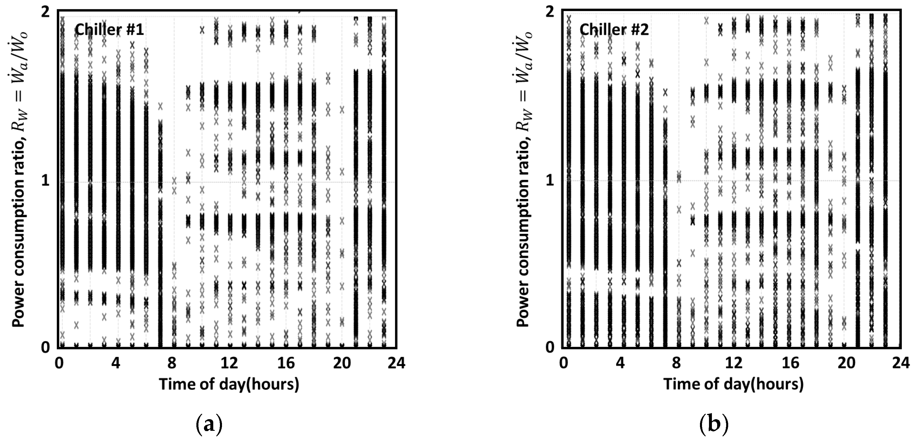
3.2.4. Collection of Chiller Power Consumption
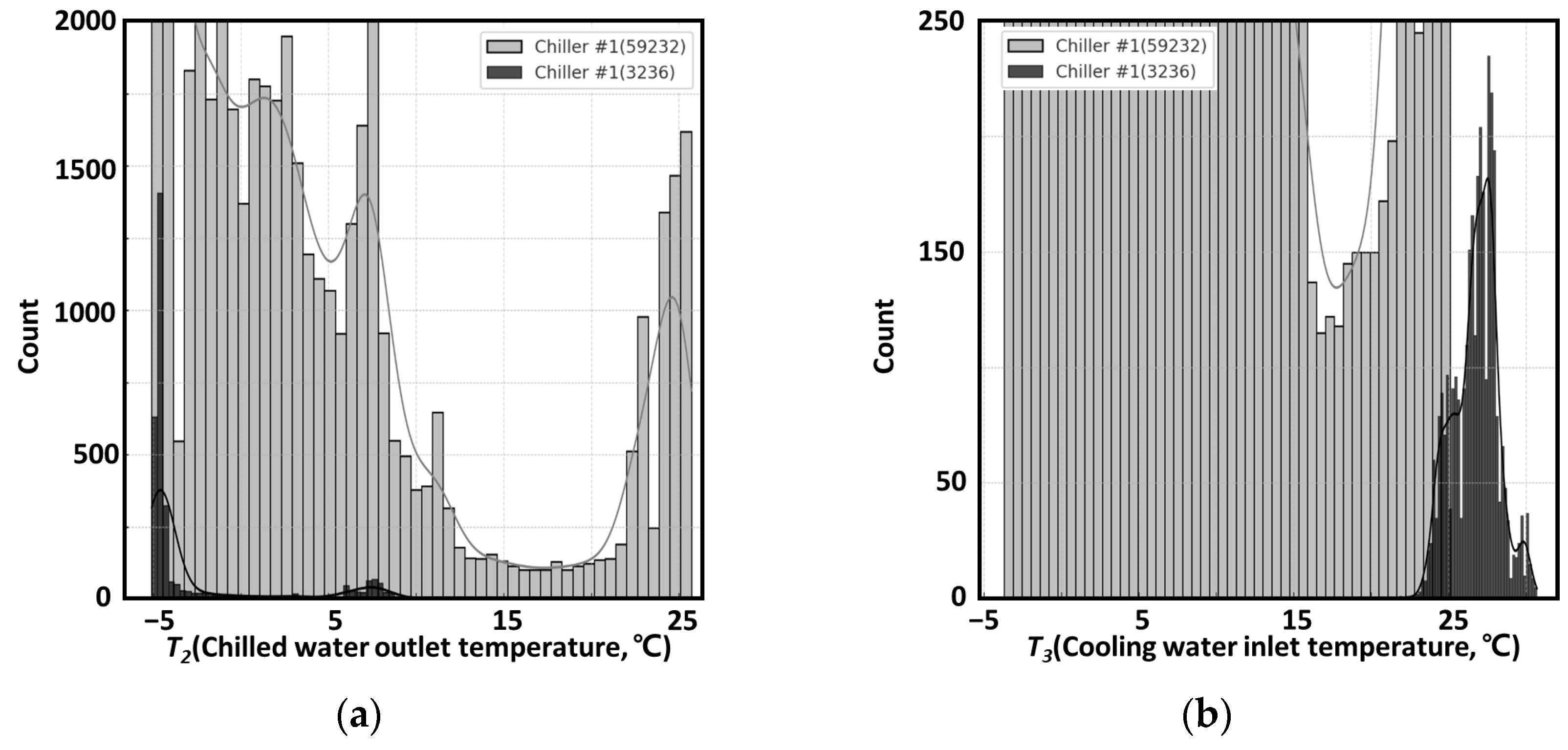
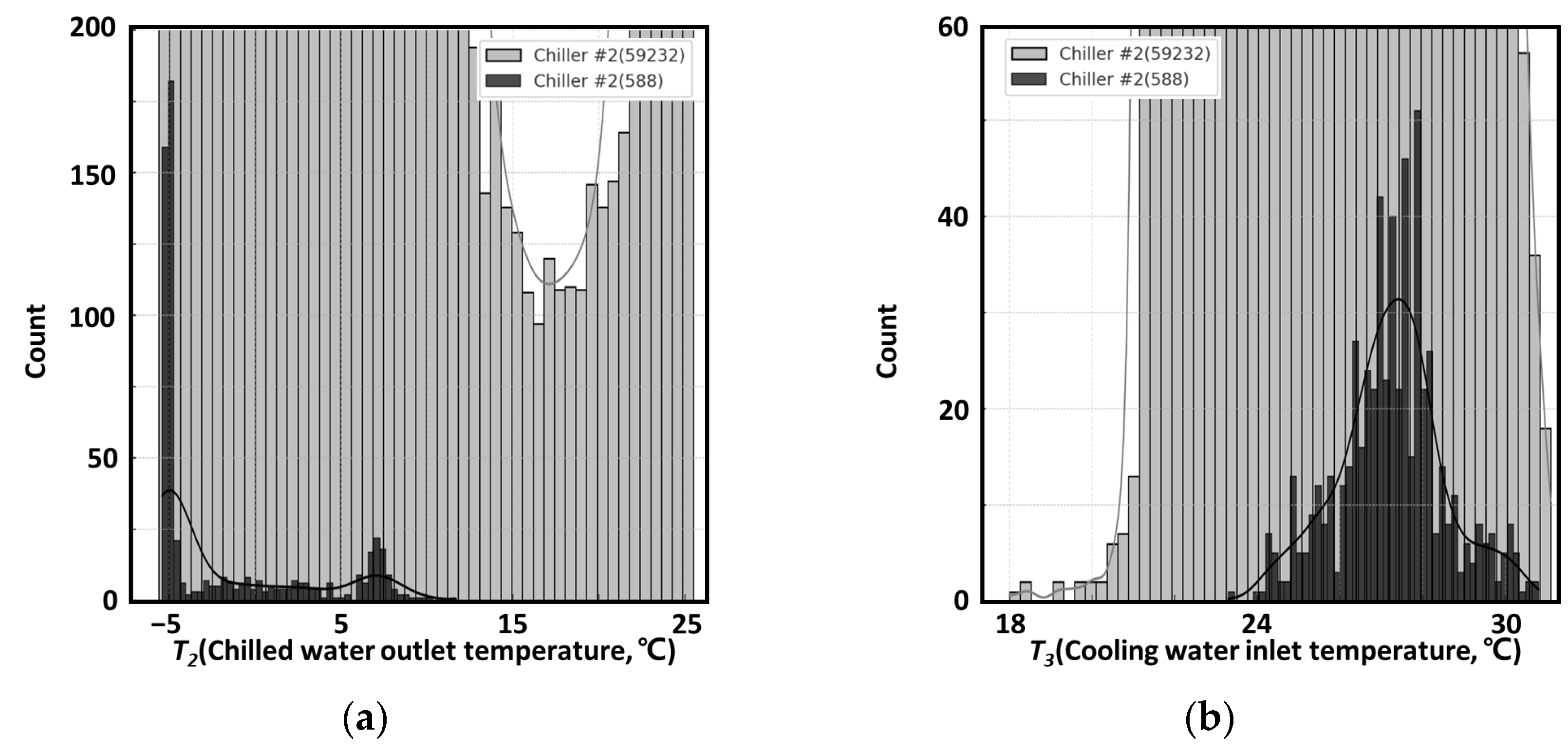
3.3. Data Preprocessing
- : The actual heat transfer exceeds the nominal heat transfer, suggesting that the chiller may be operating beyond its design conditions. This is typically caused by high load situations or unexpected changes in external environmental conditions.
- : The actual heat transfer matches the nominal heat transfer, indicating that the system is operating normally according to its design conditions.
- : The actual heat transfer is less than the nominal heat transfer, signifying that the chiller is operating under partial load. This condition is commonly observed during energy-saving modes or low-load conditions.
- : The actual performance exceeds the nominal performance, indicating that the chiller is operating more efficiently than its design conditions. This suggests optimized operating environments or ideal system operation.
- : The actual performance matches the nominal performance, signifying that the chiller is functioning normally according to its design conditions.
- : The actual performance is lower than the nominal performance, potentially indicating inefficiencies in the system, changes in external conditions, insufficient maintenance, or variations in load conditions.
3.4. Derivation of Regression Equations
3.4.1. Least Squares Regression Method (LSRM)
3.4.2. Significance Probability (p-Value)
- p-value < 0.05 (significance level);
- The null hypothesis is rejected.
- p-value ≥ 0.05;
- The null hypothesis is accepted.
3.4.3. Coefficient of Variation of Root Mean Square Error (CVRMSE)
- : The model explains 100% of the variability in the data, indicating that the predicted values () perfectly match the actual values ();
- : The model explains none of the variability in the data, and are equal to the mean of the dependent variable ();
- : The model explains part of the variability in the data, but residuals remain, indicating unexplained variability;
- : This rare case occurs when the model performs worse than simply using the mean () of the dependent variable as the prediction. It often arises from applying a linear regression model to nonlinear data or when the data structure does not align with the model.
4. Experimental Results and Discussion
4.1. Data Analysis
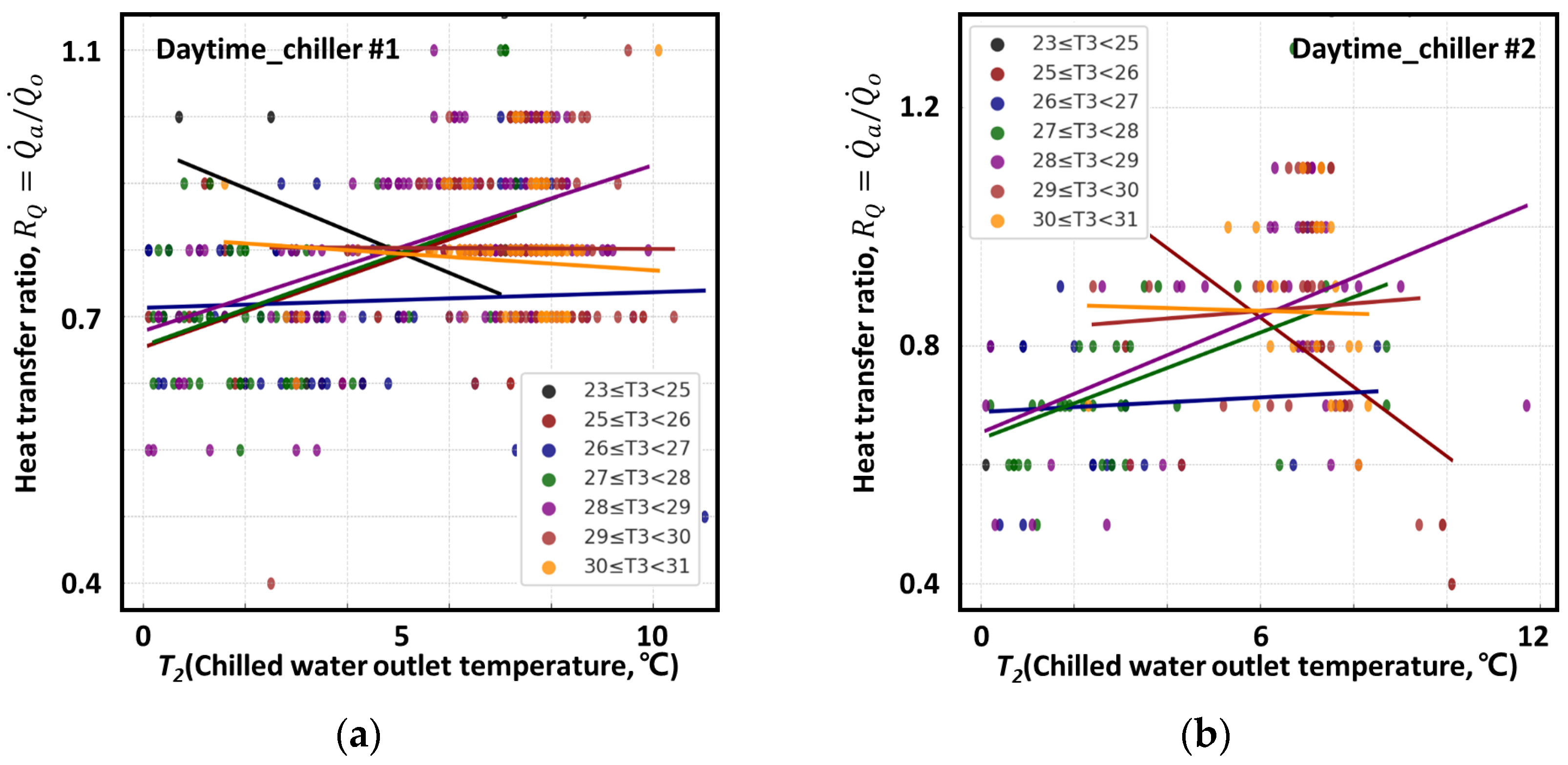
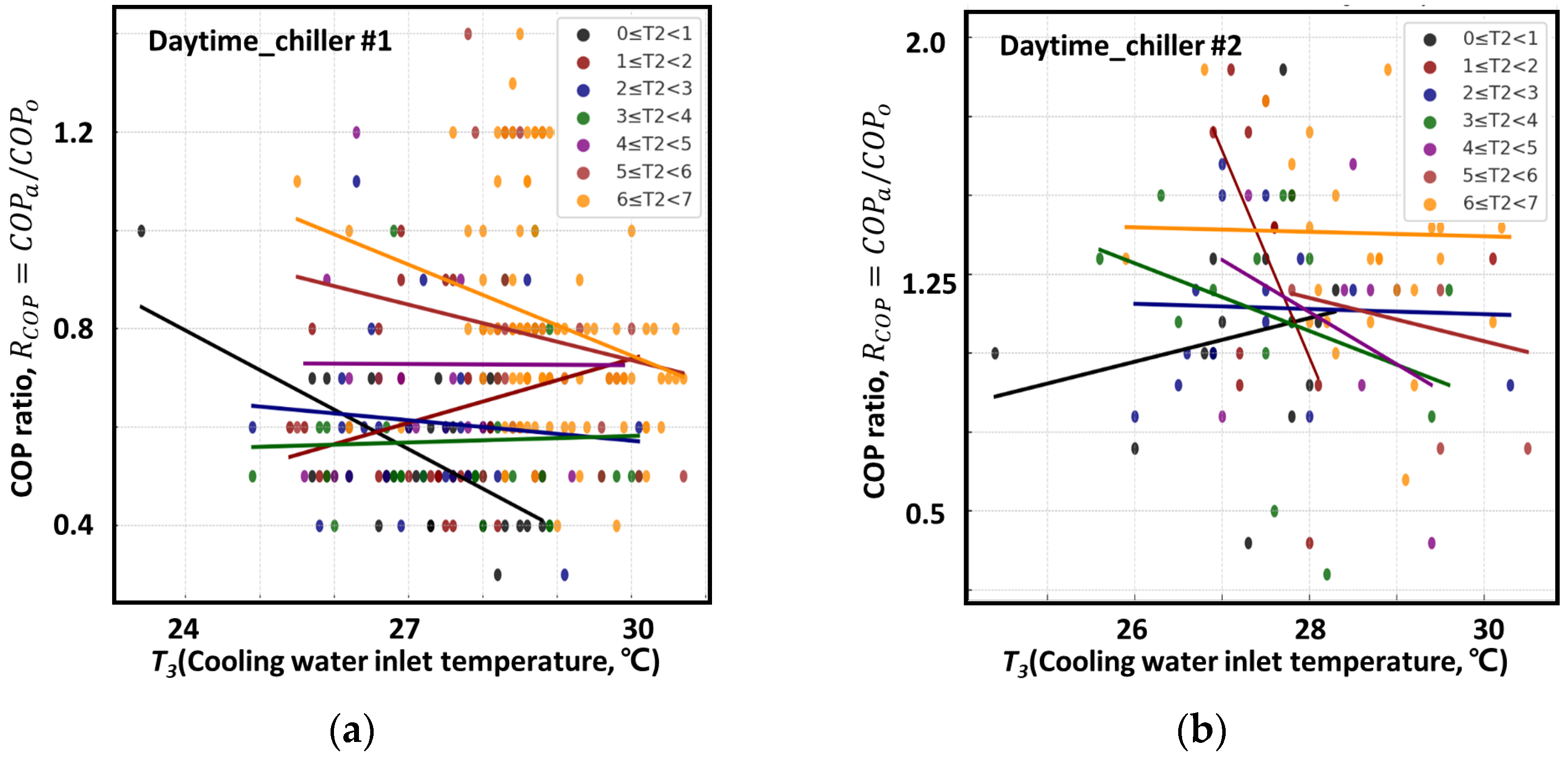
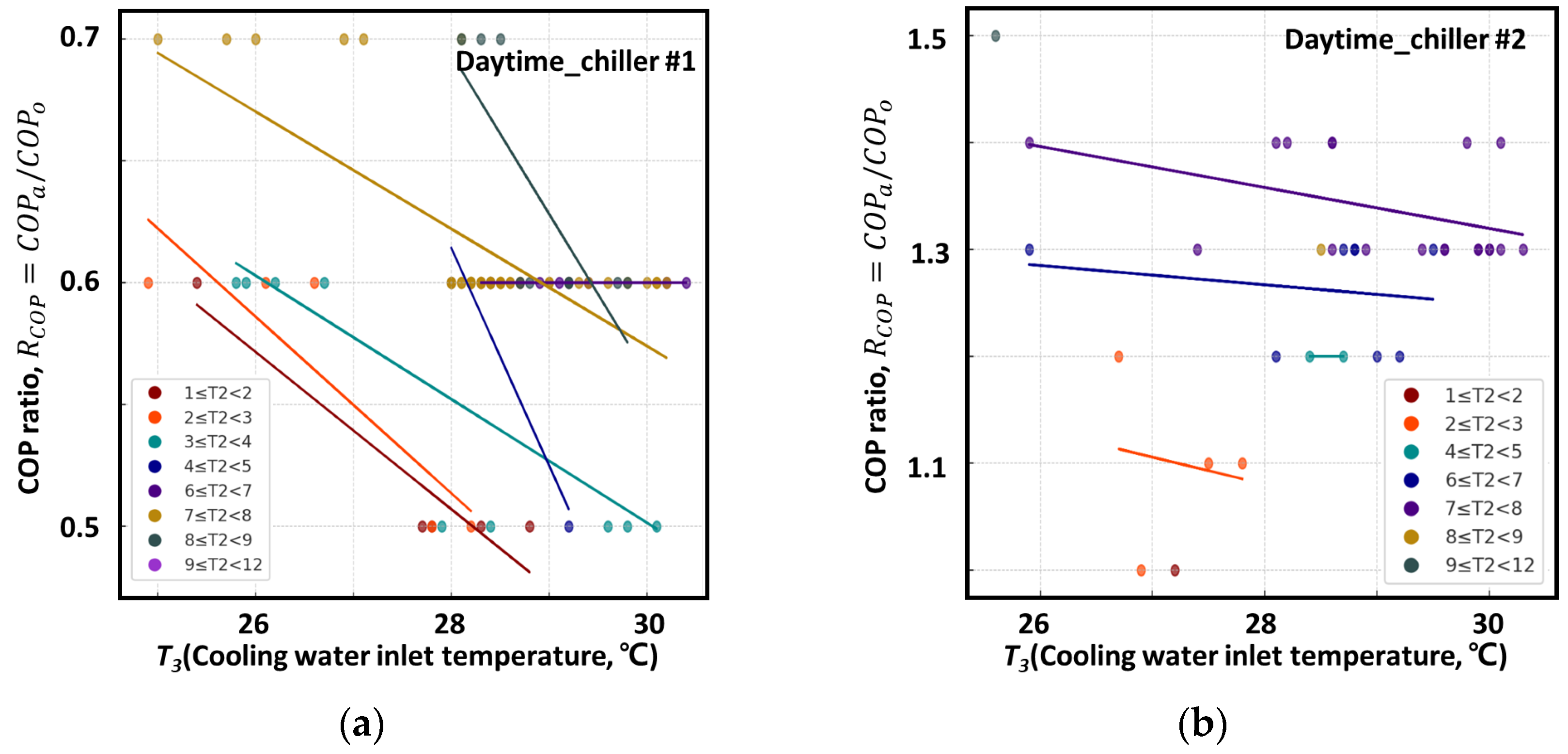
4.1.1. Daytime Analysis Results of the TRRM for Chiller #1
4.1.2. Daytime Analysis Results of the TRRM for Chiller #2
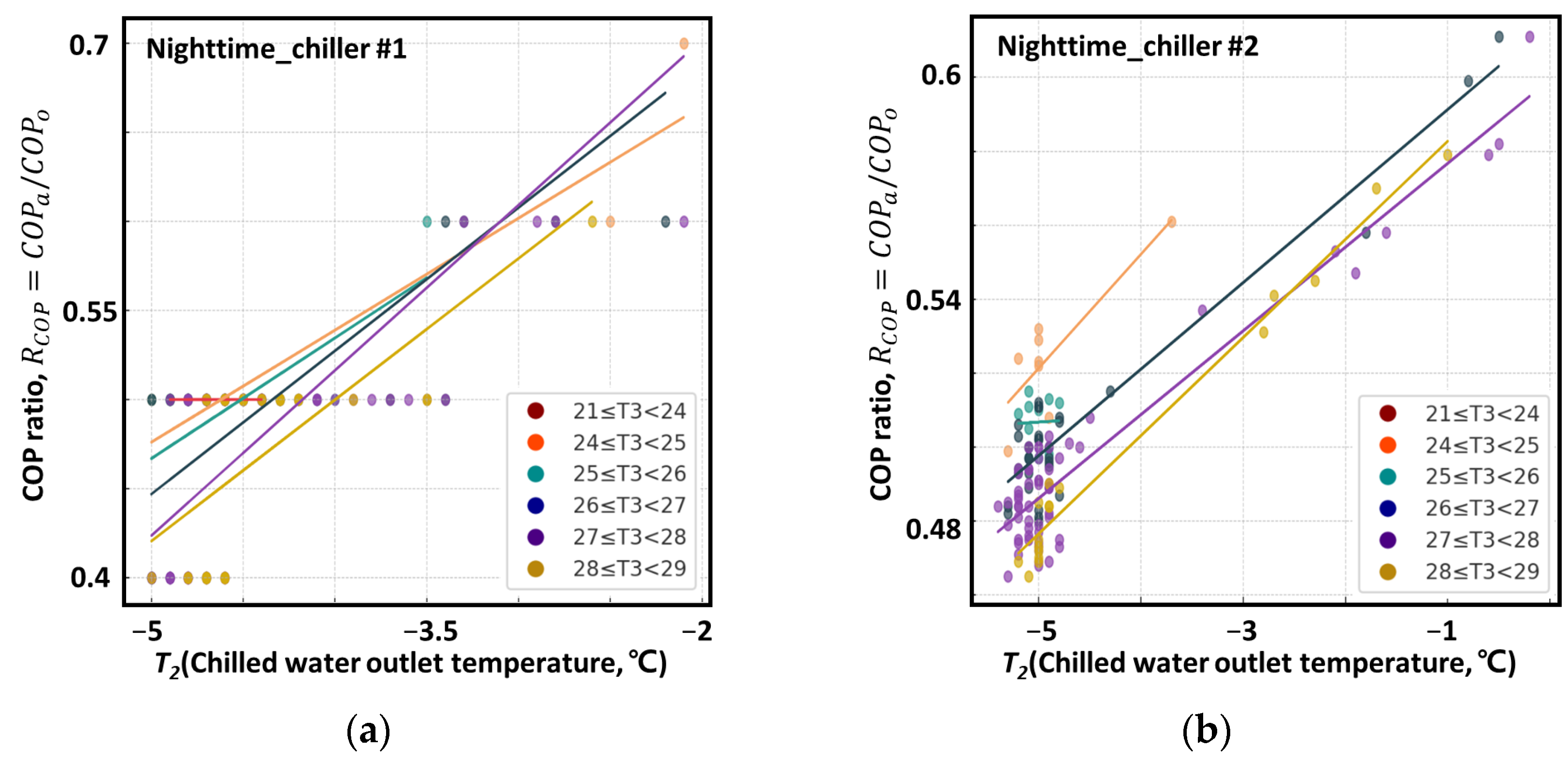
4.1.3. Nighttime Analysis Results of the TRRM for Chiller #1
4.1.4. Nighttime Analysis Results of the TRRM for Chiller #2
4.2. Validation and Comparison
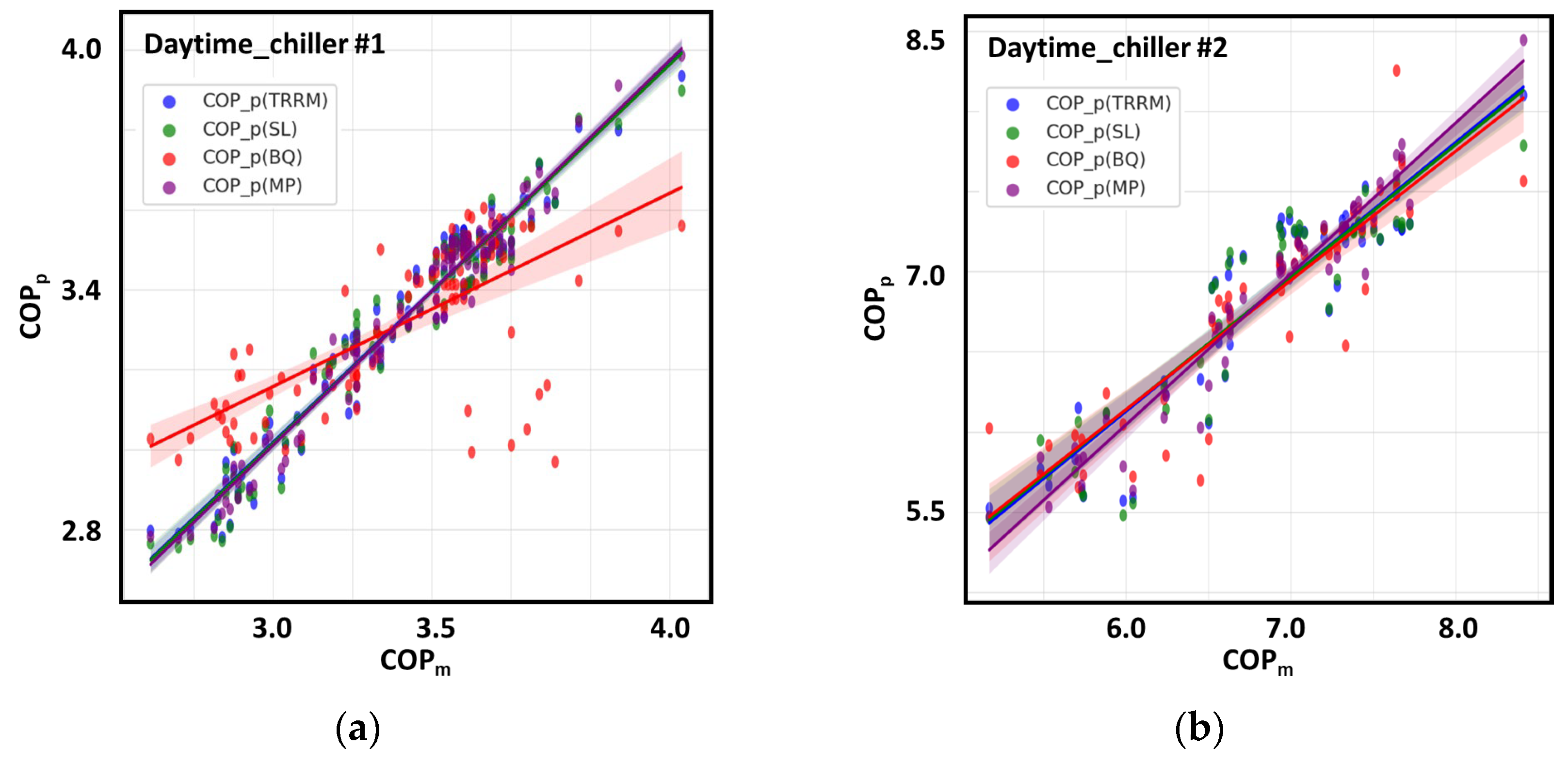
4.2.1. Validation of the Regression Model for Daytime Chiller #1 and Comparison with Alternative Models
4.2.2. Validation of the Regression Model for Daytime Chiller #2 and Comparison with Alternative Models
4.2.3. Validation of the Regression Model for Nighttime Chiller #1 and Comparison with Alternative Models
4.2.4. Validation of the Regression Model for Nighttime Chiller #2 and Comparison with Alternative Models
4.3. Prediction and Validation of COP and Error Under Standard Conditions
5. Discussion
- Diversify data collection to achieve a balance between daytime and nighttime load conditions and gather data from various buildings and regions;
- Develop thermodynamically precise models by incorporating the measurement of physical variables, such as refrigerant states (pressure and temperature);
- Introduce advanced modeling approaches, such as nonlinear regression or machine learning-based models (e.g., neural networks, ensemble learning), to enhance model accuracy and predictive capability.
6. Conclusions
- Case 1 showed the lowest error at 3.5% for chiller #1–2 daytime, while the highest error was 16.7% for chiller #1 nighttime;
- Case 2 had the lowest error at 0.6% for chiller #2 daytime and the highest at 4.5% for chiller #1 daytime;
- Case 3 exhibited an error rate of 3.7% for both chiller #1 and chiller #2;
- Case 4 recorded an error of 0.4% for chiller #2 and 4.4% for chiller #1.
Author Contributions
Funding
Data Availability Statement
Conflicts of Interest
Nomenclature
| COP | Coefficient of performance (-) |
| COPa | Actual COP (-) |
| COPo | Nominal COP (-) |
| COPp | Predicted daytime COP (-) |
| COPm | Mean COP (-) |
| increases by 1 °C, the predicted COP (-) | |
| increases by 1 °C, the predicted COP (-) | |
| TRRM | Thermo-regulated residual refinement regression model |
| EB | Energy balance (%) |
| SL model | Simple linear regression model |
| BQ model | Bi-quadratic regression model |
| MP model | Multivariate polynomial regression model |
| BEMS | Building energy management system |
| RSS | Residual sum of squares |
| MSE | Mean squared error |
| RMSE | Root mean square error |
| CVRMSE | Coefficient of variation of the root mean squared error |
| Coefficient of determination | |
| Heat transfer ratio (-) | |
| Power consumption ratio (-) | |
| COP ratio (-) | |
| Chilled water circulation flow ratio (-) | |
| Cooling water circulation flow ratio (-) | |
| Standard deviation | |
| Rate of heat transfer (kW) | |
| Rate of heat transfer on the evaporator side (kW) | |
| Rate of heat transfer on the condenser side (kW) | |
| Actual heat transfer (kW) | |
| Nominal heat transfer (kW) | |
| Power consumed by the compressor (kW) | |
| Actual power consumption (kW) | |
| Nominal power consumption (kW) | |
| Fluid density (kg/m3) | |
| Specific heat of fluid (kJ/kg°C) | |
| Specific heat of water (kJ/kg°C) | |
| Specific heat of brine (kJ/kg°C) | |
| Volumetric flow rate (L/min) | |
| Chilled water volumetric flow rate (L/min) | |
| Cooling water volumetric flow rate (L/min) | |
| Actual chilled water circulation volumetric flow (L/min) | |
| Nominal chilled water circulation volumetric flow (L/min) | |
| Actual cooling water circulation volumetric flow (L/min) | |
| Nominal cooling water circulation volumetric flow (L/min) | |
| Fluid temperature difference (°C) | |
| Chilled water inlet temperature (°C) | |
| Chilled water outlet temperature (°C) | |
| Cooling water inlet temperature (°C) | |
| Cooling water outlet temperature (°C) | |
| Actual value (observed value) | |
| Model’s estimated value (predicted value) | |
| Mean of the measured values | |
| Independent variables | |
| Regression coefficients | |
| Estimation error (residuals) | |
| Number of data points | |
| Mean of the data | |
| Total uncertainty |
References
- Korean Society of Air-Conditioning and Refrigerating Engineers (SAREK). Handbook of Air-Conditioning and Refrigeration, 4th ed.; SAREK: Seoul, Republic of Korea, 2007. [Google Scholar]
- Korean Meteorological Administration. 2023 Abnormal Climate Report; Korea Meteorological Administration: Daejeon, Republic of Korea, 2024.
- Kim, Y.I. Performance of a Water-Cooled Chiller by Controlling Chilled Water Exit Temperature. In Proceedings of the SAREK 2010 Summer Annual Conference, Pyeongchang, Republic of Korea, 23–25 June 2010; pp. 1136–1141. [Google Scholar]
- Shin, Y.G.; Chang, Y.S.; Kim, Y.I. Prediction of Vapor-Compressed Chiller Performance Using ANFIS Model. Trans. Korean Soc. Mech. Eng. B 2001, 89–95. [Google Scholar]
- Wang, H.D. A Steady-State Empirical Model for Evaluating Energy Efficient Performance of Centrifugal Water Chillers. Energy Build. 2017, 154, 415–429. [Google Scholar] [CrossRef]
- Tian, C.C.; Xing, Z.X.; Pan, X.; Tian, Y.F. A Method for COP Prediction of an On-Site Screw Chiller Applied in Cinema. Int. J. Refrig. 2019, 98, 459–467. [Google Scholar] [CrossRef]
- Lyu, Y.; Jin, X.Q.; Xue, Q.; Jia, Z.Y.; Du, Z.M. An Optimal Configuration Strategy of Multi-Chiller System Based on Overlap Analysis and Improved GA. Build. Environ. 2024, 266, 112117. [Google Scholar] [CrossRef]
- Ho, W.T.; Yu, F.W. Improved Model and Optimization for the Energy Performance of Chiller System with Diverse Component Staging. Energy 2021, 217, 119376. [Google Scholar] [CrossRef]
- Ho, W.T.; Yu, F.W. Predicting Chiller System Performance Using ARIMA-Regression Models. J. Build. Eng. 2021, 33, 101871. [Google Scholar] [CrossRef]
- Iguchi, K.; Nakayama, M.; Akisawa, A. Method for Estimating Optimum Cycle Time Based on Adsorption Chiller Parameters. Int. J. Refrig. 2019, 105, 66–71. [Google Scholar] [CrossRef]
- Nisa, E.C.; Kuan, Y.D. Comparative Assessment to Predict and Forecast Water-Cooled Chiller Power Consumption Using Machine Learning and Deep Learning Algorithms. Sustainability 2021, 13, 744. [Google Scholar] [CrossRef]
- Wang, H.D. Empirical Model for Evaluating Power Consumption of Centrifugal Chillers. Energy Build. 2017, 140, 359–370. [Google Scholar] [CrossRef]
- Lee, T.S.; Lu, W.C. An Evaluation of Empirically-Based Models for Predicting Energy Performance of Vapor-Compression Water Chillers. Appl. Energy 2010, 87, 3486–3493. [Google Scholar] [CrossRef]
- Hong, S.E. Refrigeration Engineering; Sejin Publishing: Seoul, Republic of Korea, 2018. [Google Scholar]
- Chang, Y.S.; Shin, Y.; Kim, Y.I.; Baik, Y.J. In-Situ Performance Analysis of Centrifugal Chiller According to Varying Conditions of Chilled and Cooling Water. Trans. Korean Soc. Mech. Eng. B 2002, 26, 482–490. [Google Scholar]
- Çengel, Y.A. Fundamentals of Thermal-Fluid Sciences, 5th ed.; McGraw Hill Education: New York, NY, USA, 2015; p. 253. [Google Scholar]
- Shin, Y.G.; Yang, H.C.; Tae, C.S.; Cho, S.; Kim, Y.I. In-Situ Measurement of Chiller Performance and Thermal Storage Density of an Ice Thermal Storage System. J. Korean Soc. Mech. Eng. 2005, 17, 1204–1209. [Google Scholar]
- Kim, C.D.; Lee, H.K.; Lee, Y.D.; Jeong, J.H. Performance Test of R134a Turbochiller—Part 1: Test Process. In Proceedings of the Summer Annual Conference of the Society of Air-Conditioning and Refrigerating Engineers of Korea, Pyeongchang, Republic of Korea, June 1999; pp. 1048–1053. Available online: https://www.auric.or.kr/user/search/site/sarek2016/doc_rdoc.asp?usernum=0&seid=&QU=R134a%20%C5%CD%BA%B8%B3%C3%B5%BF%B1%E2&PrimaryKey=59742&BrsDataBaseName=RDOC&DBNM=RD_R (accessed on 31 December 2024).
- Lee, D.B.; Jeong, S.K. State Equation Modeling for the Optimum Control of the Refrigeration Cycle. In Proceedings of the Society of Air-Conditioning and Refrigerating Engineers of Korea 2012 Winter Conference, Pyeongchang, Republic of Korea, November 2012; pp. 424–427. [Google Scholar]
- Reddy, T.A.; Andersen, K.K. An Evaluation of Classical Steady-State Off-Line Linear Parameter Estimation Methods Applied to Chiller Performance Data. HVAC Res. 2002, 8, 101–124. [Google Scholar] [CrossRef]
- Liu, P.L.; Chuang, B.S.; Lee, W.S.; Yeh, P.L. An Analytical Solution of the Optimal Chillers Operation Problems Based on ASHRAE Guideline 14. J. Build. Eng. 2022, 46, 103800. [Google Scholar] [CrossRef]
- Jiang, W.; Reddy, T.A. Reevaluation of the Gordon–Ng Performance Models for Water-Cooled Chillers. ASHRAE Trans. 2003, 109, 272–287. [Google Scholar]
- Sreedharan, P.; Haves, P. Comparison of Chiller Models for Use in Model-Based Fault Detection; LBNL-48149; Lawrence Berkeley National Laboratory: Austin, TX, USA, 2001.
- Swider, D.J. A Comparison of Empirically Based Steady-State Models for Vapor-Compression Liquid Chillers. Appl. Therm. Eng. 2003, 23, 539–552. [Google Scholar] [CrossRef]
- Yik, F.H.W.; Lam, V.K.C. Chiller Model for Plant Design Studies. Build. Serv. Eng. Res. Technol. 1998, 19, 233–247. [Google Scholar] [CrossRef]
- Reddy, T.A.; Niebur, D.; Andersen, K.K.; Pericolo, P.P.; Cabrera, G. Evaluation of the Suitability of Different Chiller Performance Models for On-Line Training Applied to Automated Fault Detection and Diagnosis. HVAC Res. 2003, 9, 385–408. [Google Scholar] [CrossRef]
- Department of Energy. DOE 2 Reference Manual, Part 1, Version 2.1; Lawrence Berkeley National Laboratories: Berkeley, CA, USA, 1980.
- Schurt, L.C.; Hermes, C.J.L.; Neto, A.T. A Model-Driven Multivariable Controller for Vapor Compression Refrigeration Systems. Int. J. Refrig. 2009, 32, 1672–1682. [Google Scholar] [CrossRef]
- Kim, H.; Park, C.; Lee, S. Detailed Analysis on Part Load Ratio Characteristics and Cooling Energy Saving of Chiller Staging in an Office Building under Korean Climatic Conditions. Energy Build. 2016, 127, 1012–1022. [Google Scholar]
- Palacios-Lorenzo, M.E.; Marcos, J.D. Analysis of Internal Heat Recovery Capability in Air-Cooled Indirect Fired GAX-Based Absorption Chiller in Part-Load Operation. Heliyon 2024, 10, e25656. [Google Scholar] [CrossRef] [PubMed]
- Wang, S.; Chen, Y. Online Chiller Loading Strategy Based on the Near-Optimal Performance Map for Energy Conservation. Energy Build. 2019, 183, 635–645. [Google Scholar] [CrossRef]
- ASHRAE. Guideline 14-2002. Measurement of Energy and Demand Savings; ASHRAE: Atlanta, GA, USA, 2002. [Google Scholar]
- Zhao, H.; Li, N.; Wang, S. Energy Performance Analysis of Multi-Chiller Cooling Systems for Data Centers. Build. Simul. 2022, 15, 789–802. [Google Scholar]
- Ho, W.T.; Yu, F.W. Chiller System Optimization Using k-Nearest Neighbour Regression. J. Clean. Prod. 2021, 303, 127050. [Google Scholar] [CrossRef]
- Jin, J.T.; Seok, Y.J.; Cho, H.J.; Choi, S.G.; Hwang, D.K. Design of Chilled Water Temperature Condition of Large Temperature Differential Chiller for Saving Building Energy. Korean J. Air-Cond. Refrig. Eng. 2023, 35, 90–98. [Google Scholar]


| Category | Ultrasonic Flow Meter | Temperature Sensor | AC Power Meter |
|---|---|---|---|
| Manufacturer | AutoFLO | Hankyung electric | BMT |
| Model | AUDS-100M | NT-320G | GEMS3512 |
| Measurement principle | Transit time | Insertion type | CT or Rogowski coil |
| Measurement range | ±0.02~15 m/s | −50~150 °C | 0~415 VAC |
| Error | ±1% | ±0.5% | ±0.5% |
| Category | Daytime | Nighttime | ||
|---|---|---|---|---|
| Design Conditions | Standard Conditions | Design Conditions | Standard Conditions | |
| (°C) | 12 | 12 | −0.76 | - |
| (°C) | 6.9 | 7 | −4.5 | - |
| (°C) | 31 | 32 | 30 | - |
| (°C) | 36 | 37 | 33.8 | - |
| (L/min) | 4736 | - | 4878 | - |
| (L/min) | 5196 | - | 5352 | - |
| (kW) | 286.3 | - | 268 | - |
| (kW) | 1583 | - | 1161 | - |
| COP | 5.54 | - | 4.32 | - |
| Parameters | Chiller #1 | Chiller #2 | ||||
|---|---|---|---|---|---|---|
| 59,232 (710) Datasets | 59,232 (3114) Datasets | |||||
| Min | Mean | Max | Min | Mean | Max | |
| (°C) | −3.7 (2.6) | 5.1 (9.8) | 25.1 (14.9) | −3.7 (−3.6) | 5.4 (−2.2) | 25.3 (3.8) |
| (°C) | −5.1 (0.1) | 4.2 (5.8) | 25.7 (11.7) | −5.6 (−5.4) | 4.1 (−4.4) | 25.5 (−0.1) |
| (°C) | 17.4 (23.4) | 25.2 (28.4) | 30.9 (30.8) | 18 (21.8) | 25.4 (26.5) | 31.1 (28.7) |
| (°C) | 17.7 (27.6) | 26.2 (32.7) | 35.6 (35.3) | 18.6 (24.4) | 26.2 (29.1) | 35.6 (32.3) |
| (L/min) | 70 (3495) | 4421 (4806) | 188,598 (8930) | 3903 (2930) | 4468 (4619) | 179,800 (6070) |
| (L/min) | 66 (3846) | 5178 (5472) | 226,200 (10,164) | 4020 (4188) | 5010 (5502) | 207,067 (6936) |
| (kW) | 1.0 (90) | 146.4 (318) | 11,284 (537) | 1.0 (46) | 149.3 (300) | 14,801 (459) |
| (kW) | −575.9 | 721.2 | 3569.6 | −922.7 | 905.2 | 24,849.4 |
| COPa | 130.2 (1.63) | 18.7 (4.50) | 1979.2 (10.97) | −288.9 (10.97) | 24.6 (1.11) | 24,849.4 (2.70) |
| Category | Initial Data Collection | Removed Data Containing Missing Values and Outliers | Removed Data with Energy Balance Error (±5%) | Used Data | Daytime Data (9:00–21:00) | Nighttime Data (21:00–9:00) |
|---|---|---|---|---|---|---|
| Chiller #1 | 59,232 | 45,957 | 10,039 | 3236 | 551 | 2685 |
| Chiller #2 | 59,232 | 43,134 | 15,510 | 588 | 159 | 429 |
| Total | 118,464 | 89,091 | 25,549 | 3824 | 710 | 3114 |
| Parameters | Chiller #1 | Chiller #2 | ||||||||||
|---|---|---|---|---|---|---|---|---|---|---|---|---|
| 100 Datasets | 500 Datasets | 50 Datasets | 127 Datasets | |||||||||
| Daytime | Nighttime | Daytime | Nighttime | |||||||||
| Min | Mean | Max | Min | Mean | Max | Min | Mean | Max | Min | Mean | Max | |
| (°C) | 3.4 | 9.8 | 12.8 | −3.5 | −2.4 | 1.6 | 3.2 | 9.4 | 12.7 | −3.2 | −2.0 | 3.8 |
| (°C) | 0.1 | 5.5 | 8.7 | −5.0 | −4.6 | −2.1 | 0.1 | 5.2 | 9.9 | −5.4 | −4.6 | −0.2 |
| (°C) | 24.9 | 28.2 | 30.4 | 23.3 | 26.6 | 28.5 | 24.4 | 28.4 | 30.3 | 24.3 | 27.0 | 28.6 |
| (°C) | 29.5 | 32.7 | 35.2 | 25.3 | 29.3 | 32.0 | 27.9 | 32.5 | 34.8 | 26.9 | 29.7 | 32.1 |
| (L/min) | 3670 | 5056 | 5534 | 3932 | 4852 | 5266 | 4066 | 5021 | 5534 | 4398 | 5115 | 5400 |
| (L/min) | 3732 | 5598 | 6066 | 4668 | 5658 | 6468 | 4470 | 5364 | 5802 | 5070 | 5682 | 5868 |
| (kW) | 222.0 | 408.1 | 456.0 | 250.0 | 341.9 | 441.0 | 98.0 | 205.94 | 225.0 | 140.0 | 179.5 | 222.0 |
| (kW) | 858.2 | 1359.9 | 1590.8 | 454.6 | 693.46 | 1286.5 | 801.4 | 1407.2 | 1718.1 | 720.7 | 903.0 | 1356.0 |
| (kW) | 1040.3 | 1740.1 | 2028.8 | 715.2 | 1036.4 | 1667.0 | 902.5 | 1568.1 | 1877.2 | 829.1 | 1044.9 | 1517.7 |
| COPa | 2.69 | 3.33 | 4.03 | 1.79 | 2.02 | 2.95 | 5.17 | 6.81 | 8.41 | 4.65 | 5.01 | 6.11 |
| COPTRRM,p | 2.78 | 3.33 | 3.94 | 1.83 | 2.02 | 2.88 | 5.53 | 6.81 | 8.10 | 4.70 | 5.01 | 6.03 |
| COPSL,p | 2.76 | 3.33 | 3.90 | 1.81 | 2.02 | 2.84 | 5.47 | 6.81 | 7.79 | 4.69 | 5.01 | 6.02 |
| COPBQ,p | 2.97 | 3.32 | 3.61 | 1.87 | 2.02 | 2.93 | 5.66 | 6.80 | 8.26 | 4.68 | 5.01 | 6.10 |
| COPMP,p | 2.78 | 3.33 | 3.99 | 1.82 | 2.02 | 2.95 | 5.47 | 6.81 | 8.45 | 4.71 | 5.01 | 6.07 |
| Parameter | Coefficient | |||||
|---|---|---|---|---|---|---|
| Chiller #1 | Chiller #2 | |||||
| Daytime | Nighttime | Daytime | Nighttime | |||
| TRRM | Coefficient | 6.484 | 4.575 | 6.601 | 8.604 | |
| p-value | 9.79 × 10⁻64 | 0.0000 | 8.29 × 10⁻⁹ | 5.26×10−70 | ||
| Coefficient | 0.111 | 0.317 | 0.253 | 0.182 | ||
| p-value | 8.33 × 10⁻64 | 1.42 × 10⁻259 | 1.52 × 10⁻18 | 6.44 × 10−67 | ||
| Coefficient | −0.134 | −0.041 | −0.039 | −0.120 | ||
| p-value | 8.16 × 10⁻42 | 4.27 × 10⁻103 | 0.2646 | 3.71 × 10⁻²⁸ | ||
| 0.946 | 0.916 | 0.840 | 0.915 | |||
| CVRMSE | 1.93% | 1.90% | 4.16% | 1.74% | ||
| SL | Coefficient | 6.159 | 3.606 | 6.2539 | 8.7983 | |
| p-value | 1.29 × 10⁻60 | 3.95 × 10⁻222 | 8.89 × 10⁻⁸ | 3.16 × 10−59 | ||
| Coefficient | −0.0002 | −0.000088 | −0.00014 | −0.000149 | ||
| p-value | 9.87 × 10⁻5 | 0.0272 | 0.611 | 0.2753 | ||
| Coefficient | 0.110 | 0.1987 | 0.2302 | 0.1952 | ||
| p-value | 3.10 × 10⁻55 | 2.53 × 10⁻113 | 3.65 × 10⁻13 | 4.15 × 10⁻³⁰ | ||
| Coefficient | 0.130 | −0.0390 | −0.0496 | −0.1209 | ||
| p-value | 1.08 × 10⁻39 | 1.96 × 10⁻74 | 0.207 | 3.89 × 10⁻²⁸ | ||
| 0.946 | 0.879 | 0.827 | 0.916 | |||
| CVRMSE | 1.94% | 2.27% | 4.50% | 1.74% | ||
| BQ | Coefficient | 65.630 | 29.4814 | 75.849 | −18.8377 | |
| p-value | 0.4679 | 0.1688 | 0.034 | >0.4 | ||
| Coefficient | −50,250.208 | −11,452.88 | −0.0283 | 9906.8719 | ||
| p-value | 0.3697 | 0.1256 | 0.038 | >0.4 | ||
| Coefficient | −0.022 | −0.0196 | −5.2766 | 0.0086 | ||
| p-value | 0.5411 | 0.1982 | 0.042 | >0.4 | ||
| Coefficient | 3750.860 | 897.23 | −48,198.0345 | −738.8523 | ||
| p-value | 0.3566 | 0.1172 | 0.031 | >0.4 | ||
| Coefficient | −70.242 | −17.59 | 3378.4225 | 13.6068 | ||
| p-value | 0.3412 | 0.1080 | 0.038 | >0.4 | ||
| Coefficient | −4.93 | −2.27 | −59.3091 | 1.4089 | ||
| p-value | 0.4524 | 0.1657 | 0.046 | >0.4 | ||
| Coefficient | 0.0017 | 0.00152 | 0.00197 | −0.0006 | ||
| p-value | 0.5211 | 0.1918 | 0.047 | >0.4 | ||
| Coefficient | 0.0936 | 0.0448 | 0.0922 | −0.0256 | ||
| p-value | 0.4316 | 0.1522 | 0.050 | >0.4 | ||
| Coefficient | −0.000032 | −0.00003 | −0.0000342 | 0.000011 | ||
| p-value | 0.4971 | 0.1792 | 0.056 | >0.4 | ||
| 0.476 | 0.706 | 0.781 | 0.857 | |||
| CVRMSE | 6.51% | 3.17% | 5.72% | 2.13% | ||
| Coefficient | 12.72 | 5.558 | 1.6455 | 2.5429 | ||
| p-value | 0.000007 | 0.000104 | 0.8815 | >0.16 | ||
| Coefficient | −0.000786 | 0.00250 | −0.003520 | 0.0087 | ||
| p-value | 0.4139 | 0.0768 | 0.2947 | >0.16 | ||
| Coefficient | 0.1971 | −0.0339 | −0.2371 | −0.8841 | ||
| p-value | 0.0091 | 0.8571 | 0.4988 | >0.16 | ||
| Coefficient | −0.6165 | −0.2876 | 0.4633 | −0.0519 | ||
| p-value | 0.0012 | 0.0003 | 0.5859 | >0.16 | ||
| Coefficient | 8.69 × 10⁻7 | 7.73 × 10⁻8 | 0.000007679 | −0.000002 | ||
| p-value | 0.0003 | 0.8880 | 0.00000001909 | >0.16 | ||
| Coefficient | 0.00438 | 0.0219 | 0.009683 | −0.0152 | ||
| p-value | 0.0009 | 0.0047 | 0.09659 | >0.16 | ||
| Coefficient | 0.01066 | 0.00674 | −0.004442 | 0.0015 | ||
| p-value | 0.0018 | 0.000001 | 0.7884 | >0.16 | ||
| Coefficient | −3.08 × 10⁻5 | −8.83 × 10⁻5 | −0.0005780 | 0.0005 | ||
| p-value | 0.1252 | 0.4806 | 0.0000008350 | >0.16 | ||
| Coefficient | −4.61 × 10⁻5 | −1.04 × 10⁻4 | −0.0003702 | −0.0001 | ||
| p-value | 0.1268 | 0.0019 | 0.02270 | >0.16 | ||
| Coefficient | −0.00453 | 0.0135 | 0.03336 | 0.0190 | ||
| p-value | 0.0876 | 0.0129 | 0.03521 | >0.16 | ||
| 0.963 | 0.894 | 0.942 | 0.922 | |||
| CVRMSE | 1.66% | 2.15% | 2.79% | 1.72% | ||
| Category | Daytime | Nighttime | ||||||||
|---|---|---|---|---|---|---|---|---|---|---|
| Design Conditions | Standard Conditions | Design Conditions | ||||||||
| Design Temp’ | 2 Case 1 ) | 3 Case 2 ) | Standard Temp’ | 4 Case 3 ) | 5 Case 4 ) | Design Temp’ | 2 Case 1 ) | 3 Case 2 ) | ||
| (°C) | 6.9 | 7.9 | 6.9 | 7 | 8 | 7 | −4.5 | −3.5 | −4.5 | |
| (°C) | 31 | 31 | 32 | 32 | 32 | 33 | 30 | 30 | 31 | |
| Chiller #1 | 1 COPp | 3.10 | 3.21 | 2.96 | 2.97 | 3.08 | 2.84 | 1.92 | 2.24 | 1.88 |
| (%) | −6.9% | - | - | −10.8% | - | - | −5.0% | - | - | |
| (%) | - | 3.5% | - | - | 3.7% | - | - | 16.7% | - | |
| (%) | - | - | −4.5% | - | - | −4.4% | - | - | −2.1% | |
| Chiller #2 | 1 COPp | 7.14 | 7.39 | 7.10 | 7.12 | 7.38 | 7.09 | 4.19 | 4.37 | 4.07 |
| (%) | 4.8% | - | - | 4.6% | - | - | −16.4% | - | - | |
| (%) | - | 3.5% | - | 3.7% | - | - | 4.3% | - | ||
| (%) | - | - | −0.6% | - | - | −0.4% | - | - | −2.9% | |
Disclaimer/Publisher’s Note: The statements, opinions and data contained in all publications are solely those of the individual author(s) and contributor(s) and not of MDPI and/or the editor(s). MDPI and/or the editor(s) disclaim responsibility for any injury to people or property resulting from any ideas, methods, instructions or products referred to in the content. |
© 2025 by the authors. Licensee MDPI, Basel, Switzerland. This article is an open access article distributed under the terms and conditions of the Creative Commons Attribution (CC BY) license (https://creativecommons.org/licenses/by/4.0/).
Share and Cite
Kim, S.W.; Kim, Y.I. Performance Prediction of a Water-Cooled Centrifugal Chiller in Standard Temperature Conditions Using In-Situ Measurement Data. Sustainability 2025, 17, 2196. https://doi.org/10.3390/su17052196
Kim SW, Kim YI. Performance Prediction of a Water-Cooled Centrifugal Chiller in Standard Temperature Conditions Using In-Situ Measurement Data. Sustainability. 2025; 17(5):2196. https://doi.org/10.3390/su17052196
Chicago/Turabian StyleKim, Sung Won, and Young Il Kim. 2025. "Performance Prediction of a Water-Cooled Centrifugal Chiller in Standard Temperature Conditions Using In-Situ Measurement Data" Sustainability 17, no. 5: 2196. https://doi.org/10.3390/su17052196
APA StyleKim, S. W., & Kim, Y. I. (2025). Performance Prediction of a Water-Cooled Centrifugal Chiller in Standard Temperature Conditions Using In-Situ Measurement Data. Sustainability, 17(5), 2196. https://doi.org/10.3390/su17052196