POI Data–Driven Identification and Representation of Production–Living–Ecological Spaces at the Urban and Peri–Urban Scale: A Case Study of the Hohhot–Baotou–Ordos–Yulin Urban Agglomeration


Abstract
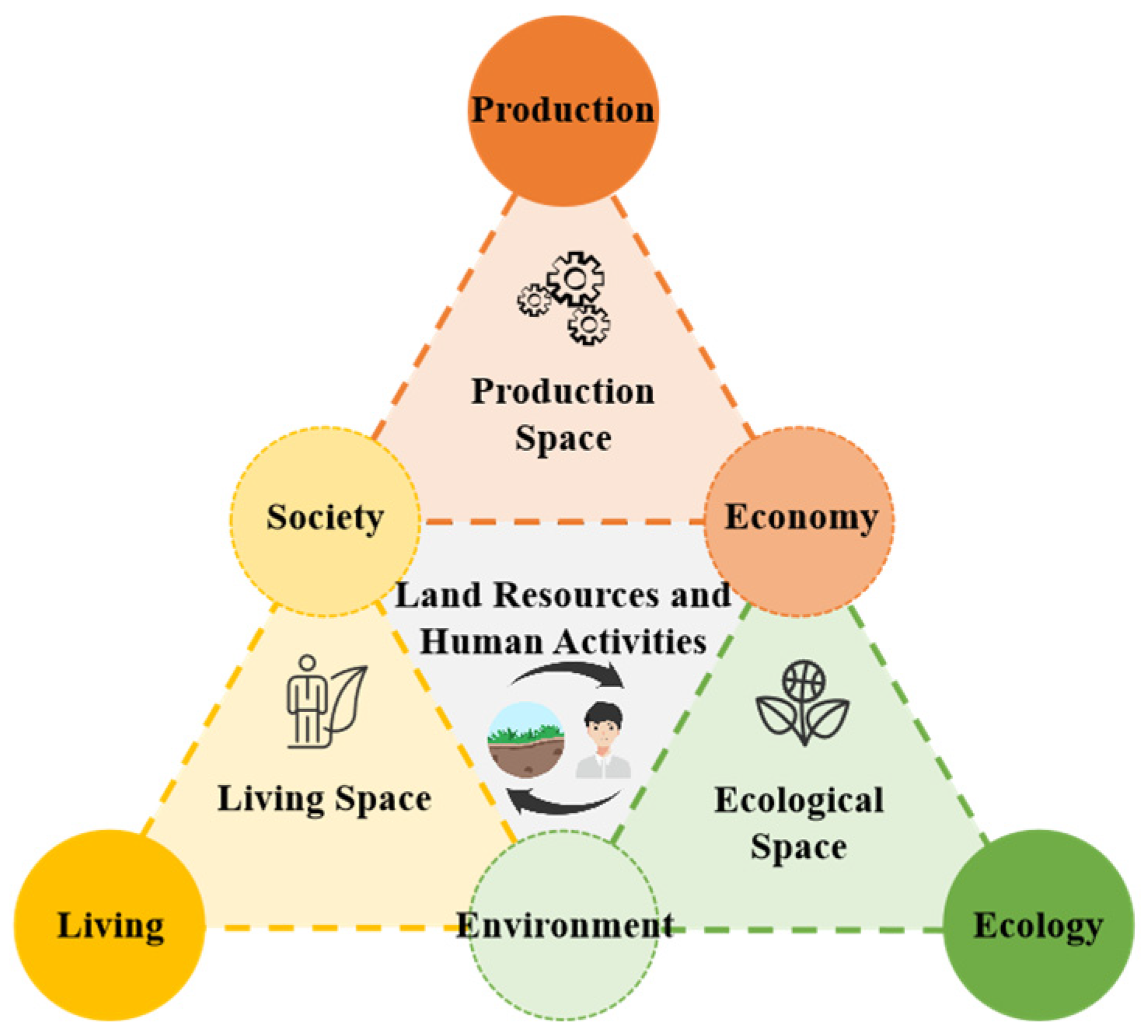
1. Introduction
2. Materials and Methods
2.1. Study Area
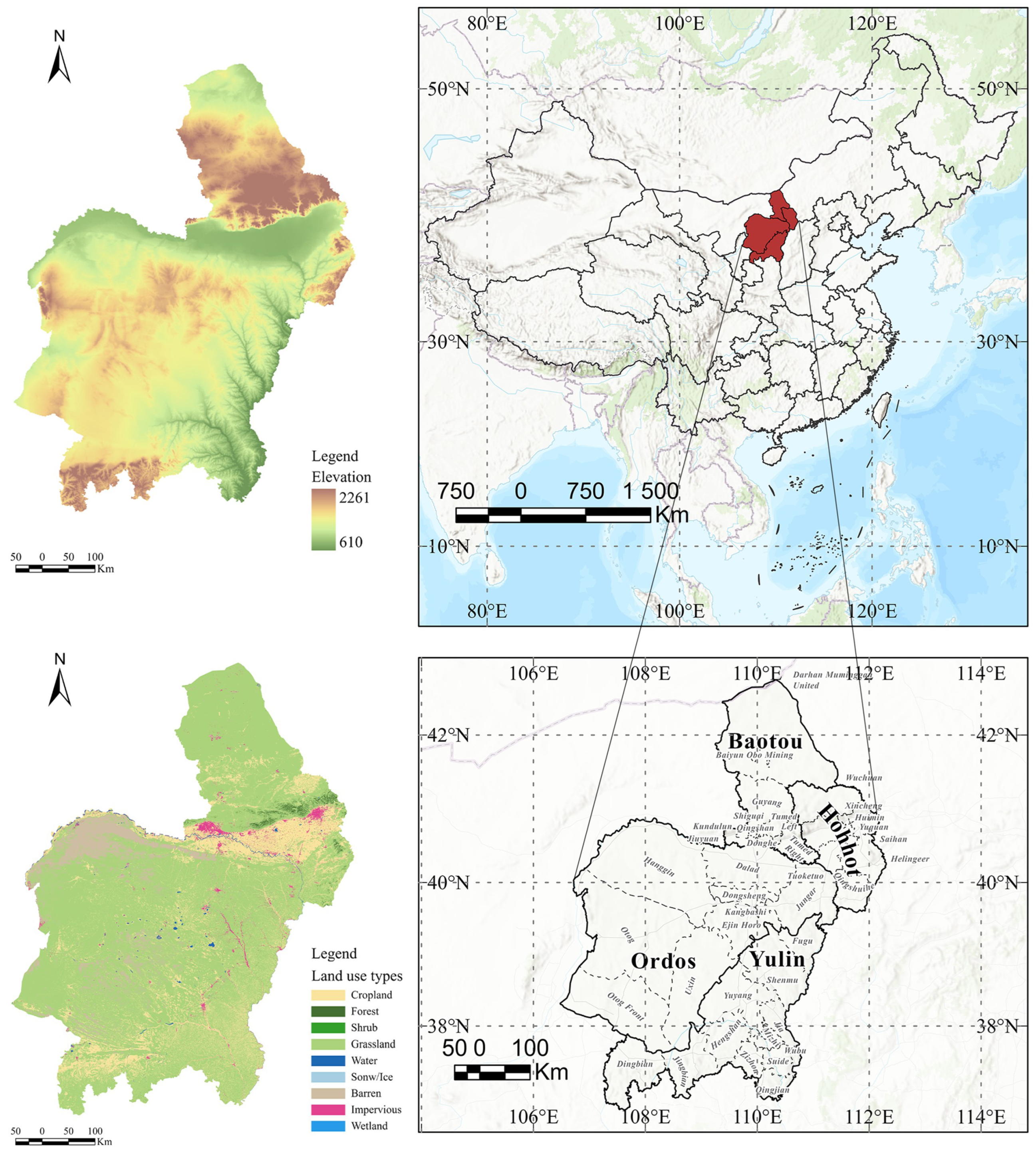
2.1.1. Overview of the Study Area
2.1.2. Data Sources and Preprocessing
- Urban Core Areas
- 2.
- Peri–Urban Areas
- 3.
- Non–Study Areas
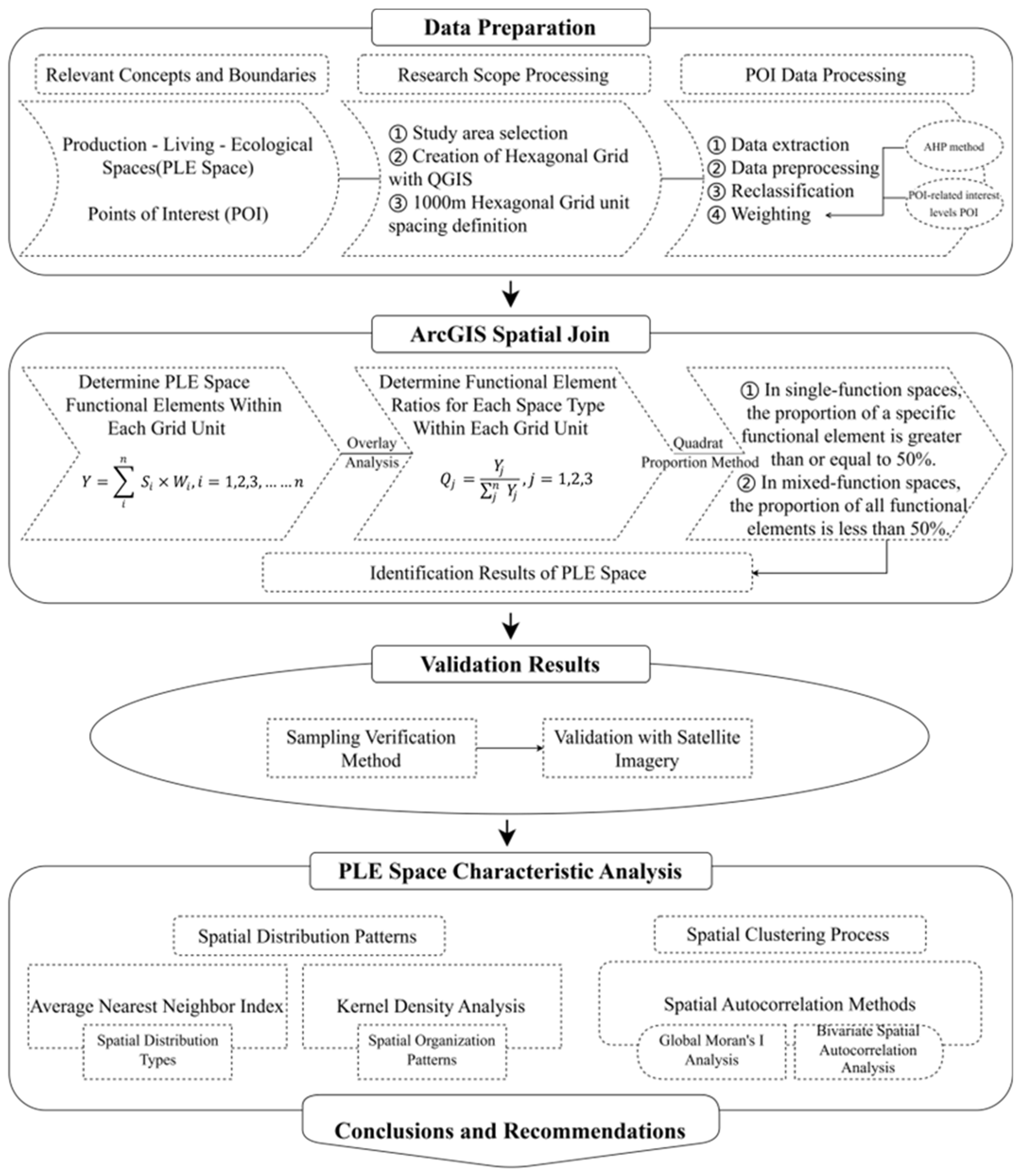
2.2. Methods
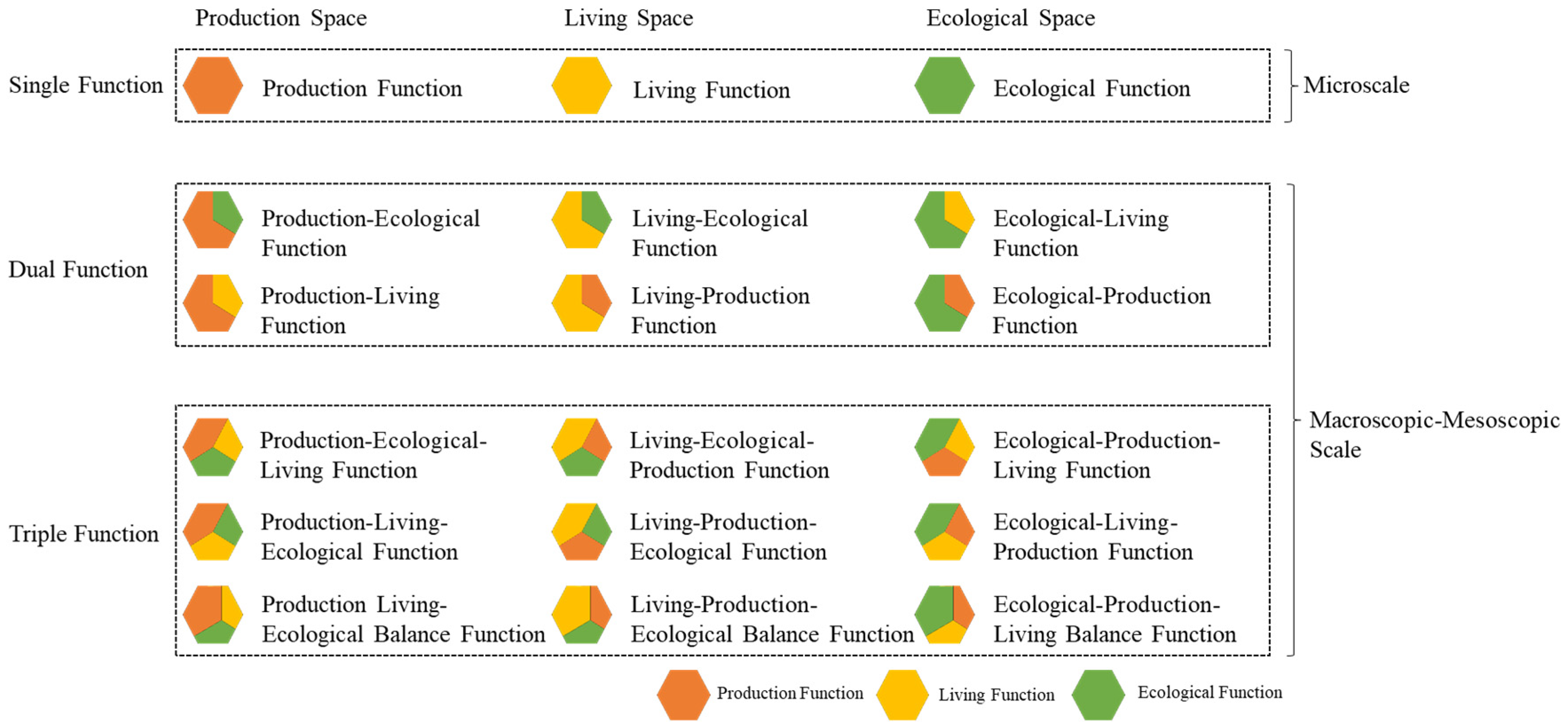
2.2.1. PLES Identification Based on POI Data
- Data Preparation and Classification System Construction
- 2.
- Comprehensive Weight Calculation
- 3.
- Spatial Integration and Function Identification
- 4.
- Result Validation
2.2.2. Spatial Pattern Analysis
- Distribution Pattern Analysis
- 2.
- Kernel Density Analysis
- 3.
- Spatial Autocorrelation Analysis
3. Results
3.1. Identification Results and Validation
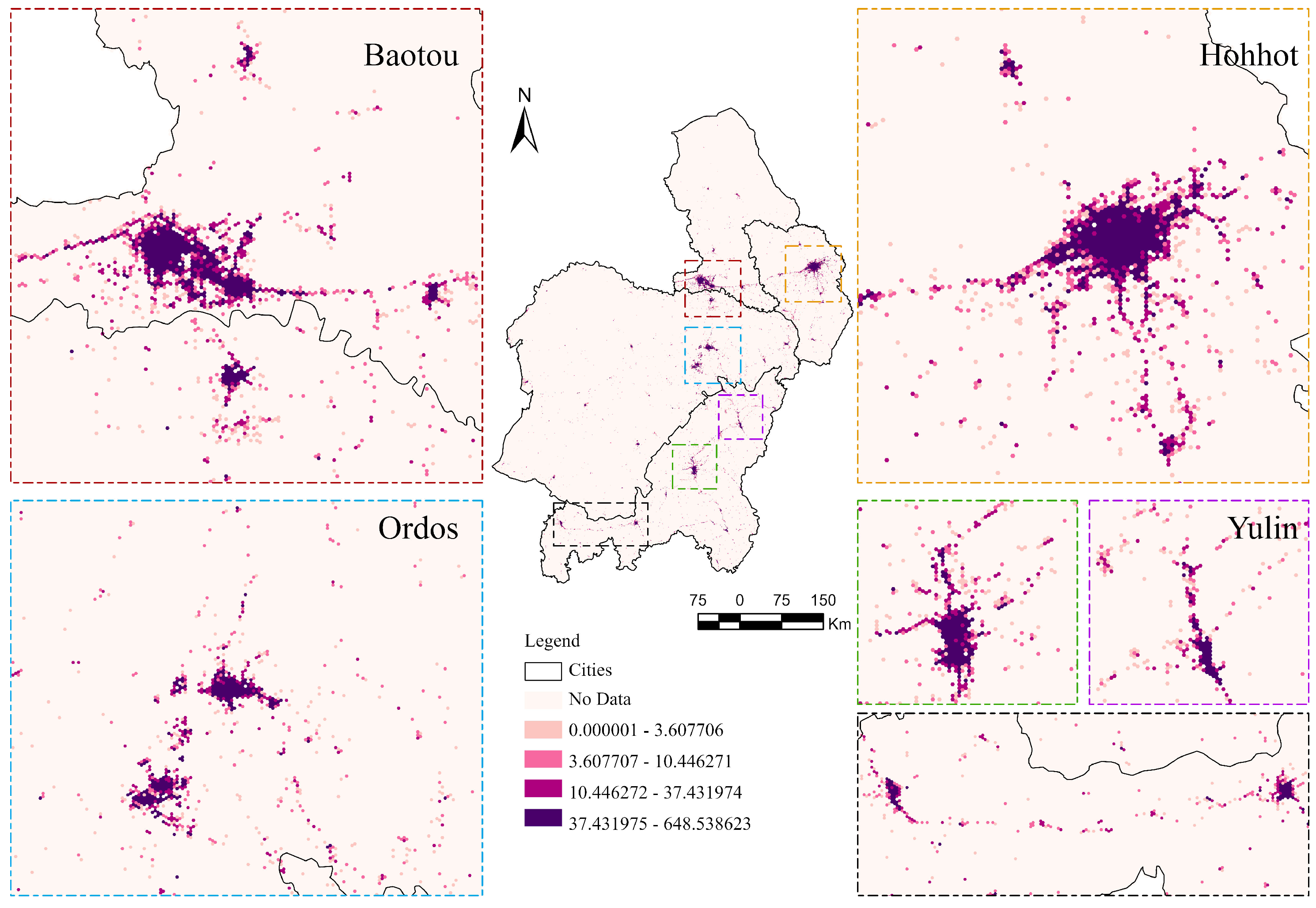
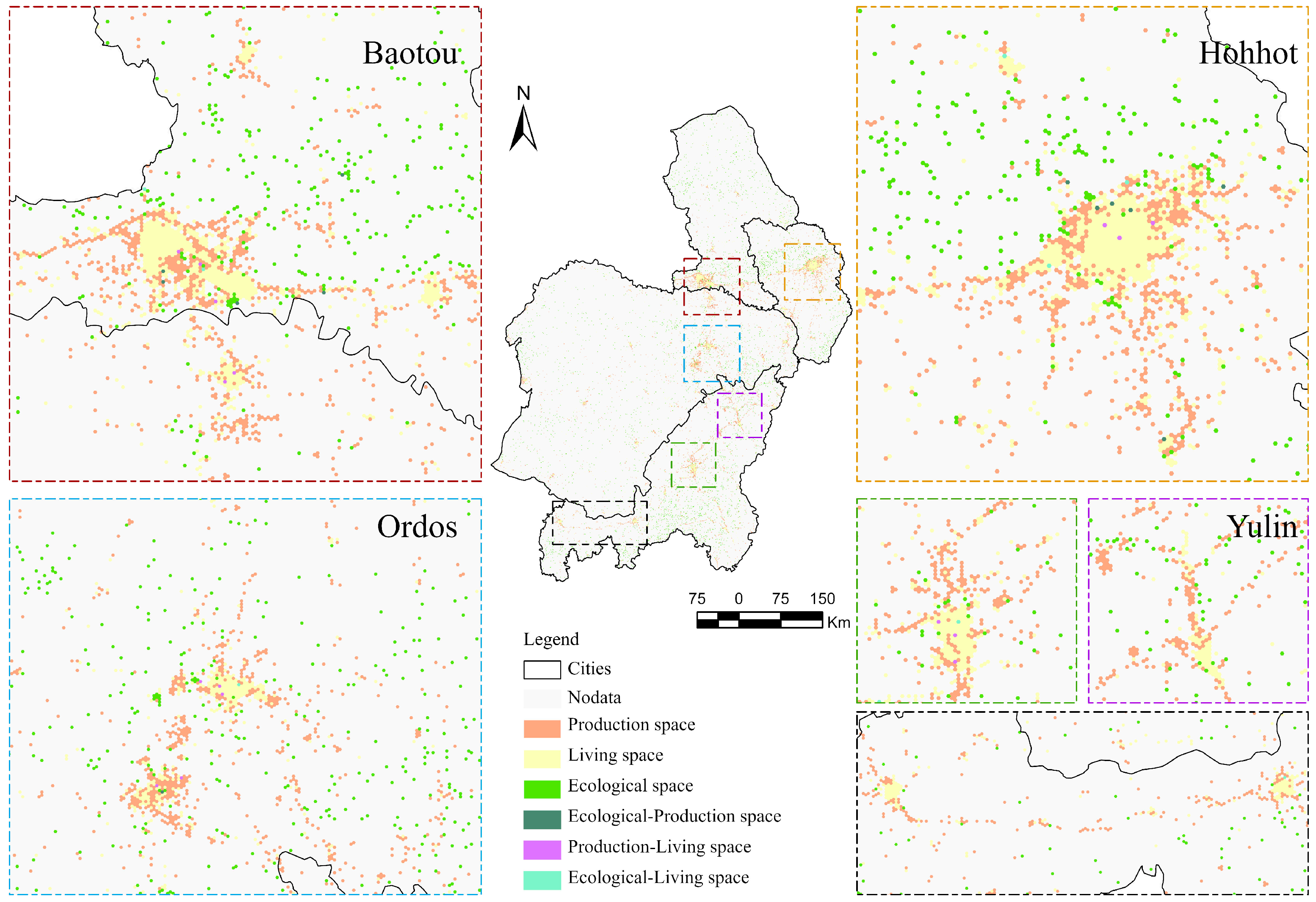
3.1.1. Identification Results of Production–Living–Ecological Spaces
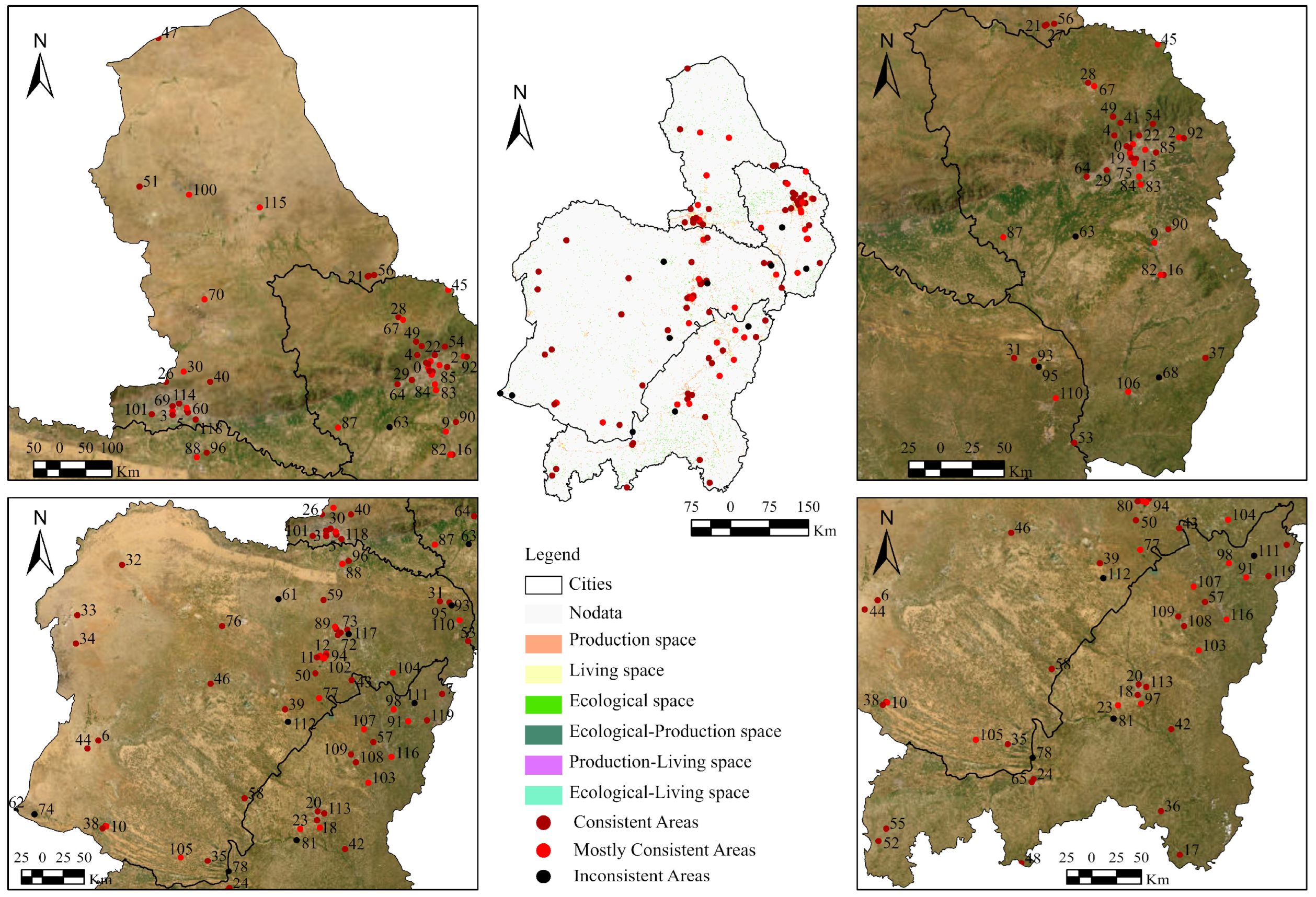
3.1.2. Validation of PLES
3.2. Spatial Distribution Analysis of PLES
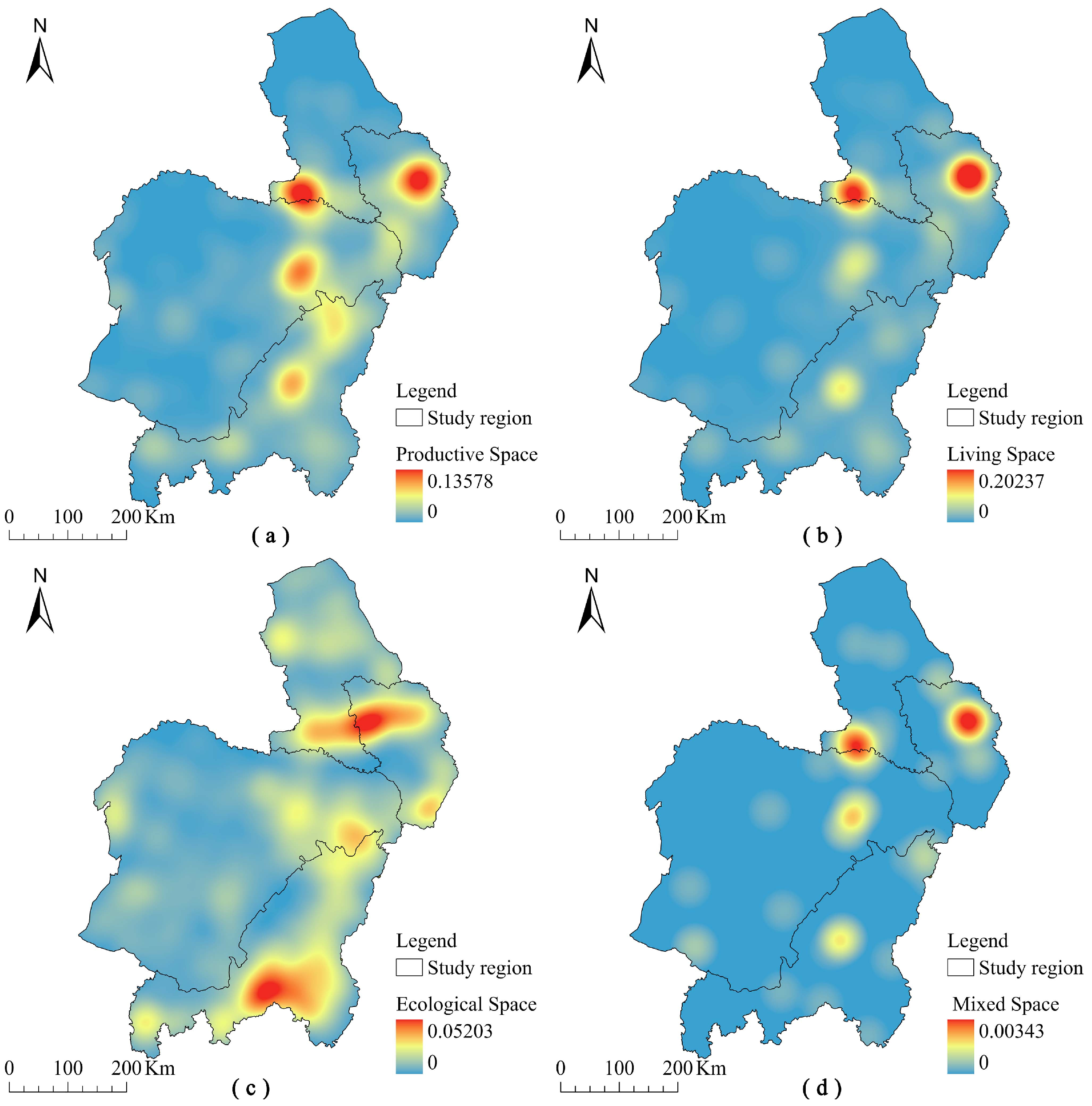
3.2.1. Spatial Distribution Types of PLES
3.2.2. Spatial Distribution Patterns of PLES
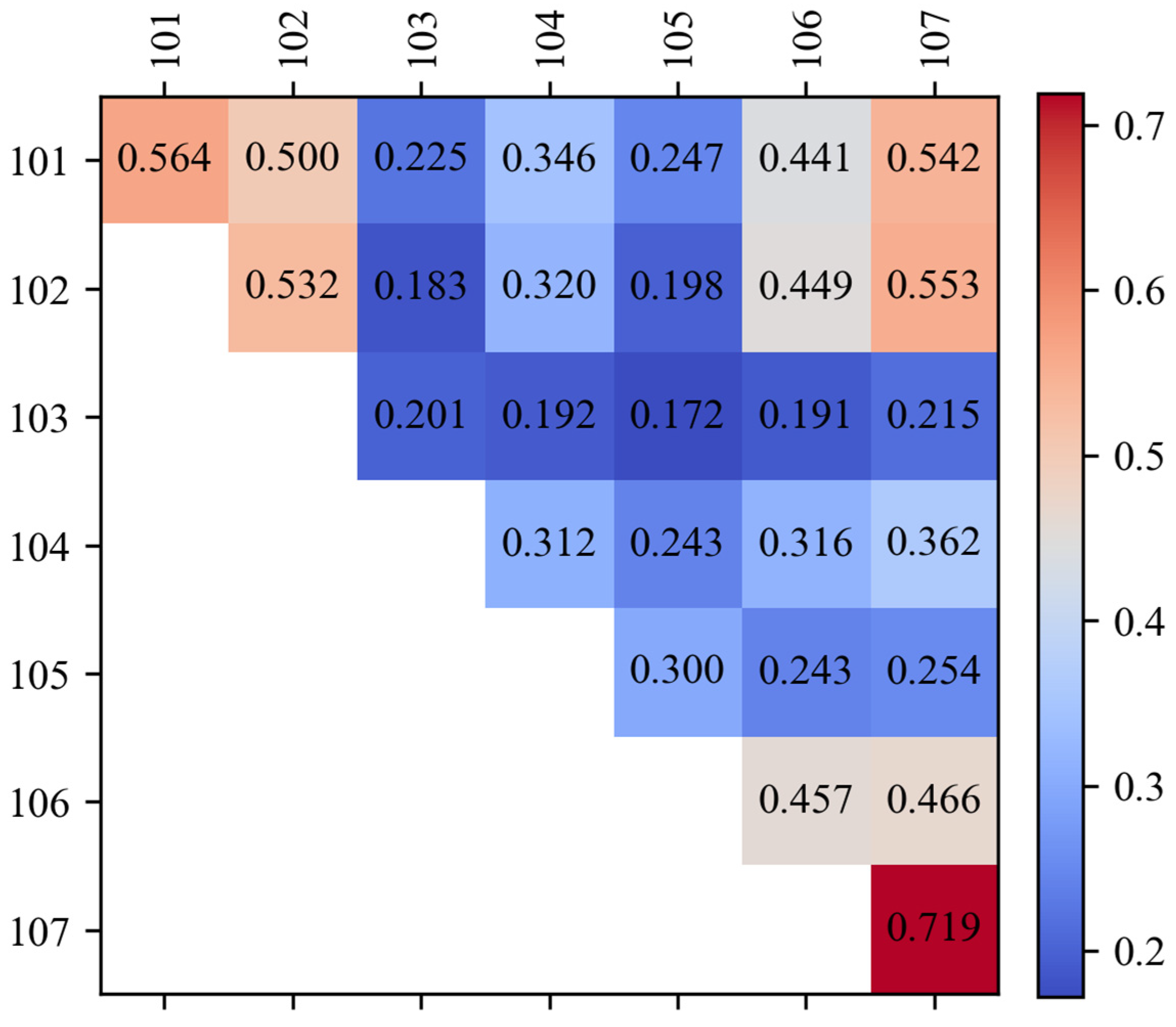
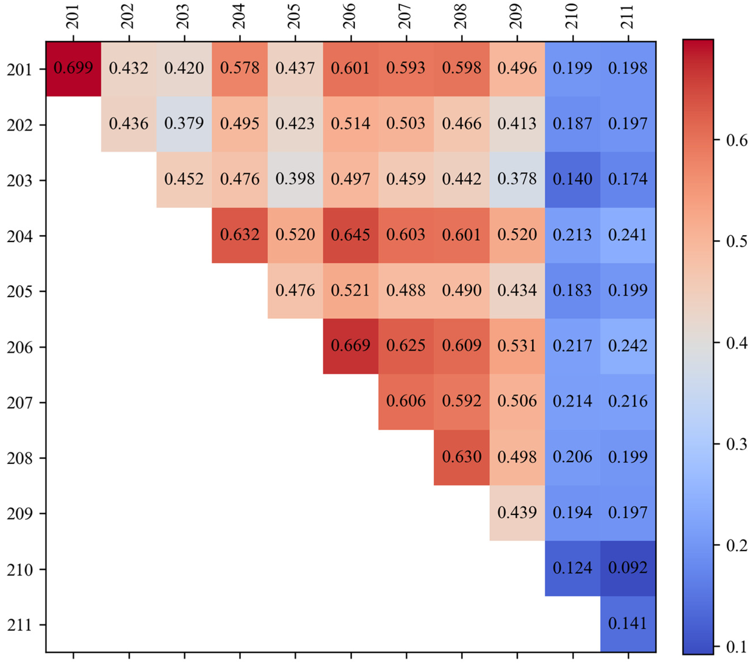
3.3. Correlation of the Distribution Characteristics of PLES
4. Discussion
4.1. Analysis of PLES Identification Results Based on POI Data and Application Advantages
4.2. Limitations and Future Prospects
5. Conclusions
Author Contributions
Funding
Institutional Review Board Statement
Informed Consent Statement
Data Availability Statement
Acknowledgments
Conflicts of Interest
References
- Wang, X.; Wang, D.; Wu, S.; Yan, Z.; Han, J. Cultivated Land Multifunctionality in Undeveloped Peri-Urban Agriculture Areas in China: Implications for Sustainable Land Management. J. Environ. Manag. 2023, 325, 116500. [Google Scholar] [CrossRef] [PubMed]
- Zhu, Y.-G.; Reid, B.J.; Meharg, A.A.; Banwart, S.A.; Fu, B.-J. Optimizing Peri-URban Ecosystems (PURE) to Re-Couple Urban-Rural Symbiosis. Sci. Total Environ. 2017, 586, 1085–1090. [Google Scholar] [CrossRef]
- Kleijn, D.; Berendse, F.; Smit, R.; Gilissen, N. Agri-Environment Schemes Do Not Effectively Protect Biodiversity in Dutch Agricultural Landscapes. Nature 2001, 413, 723–725. [Google Scholar] [CrossRef] [PubMed]
- Brunstad, R.J.; Gaasland, I.; Vårdal, E. Multifunctionality of Agriculture: An Inquiry into the Complementarity Between Landscape Preservation and Food Security. Eur. Rev. Agric. Econ. 2005, 32, 469–488. [Google Scholar] [CrossRef]
- Gafsi, M.; Nguyen, G.; Legagneux, B.; Robin, P. Sustainability and Multifunctionality in French Farms: Analysis of the Implementation of Territorial Farming Contracts. Agric. Hum. Values 2006, 23, 463–475. [Google Scholar] [CrossRef]
- Sustainable Development. Available online: https://sdgs.un.org/ (accessed on 19 November 2024).
- Huang, J.; Lin, H.; Qi, X. A Literature Review on Optimization of Spatial Development Pattern Based on Ecological-Production-Living Space. Prog. Geogr. 2017, 36, 378–391. [Google Scholar] [CrossRef]
- The Outline of the 14th Five-Year Plan for National Economic and Social Development and Long-Range Objectives for 2035 of the People’s Republic of China. People’s Daily. 13 March 2021, p. 1. Available online: https://kns.cnki.net/kcms2/article/abstract?v=MdENDFpkZq6BzDNZWFhBZ0e_WYYkU64Jq11qI_0Xu1KR_rZ-qrMFXM1ri8MIFk2CwKmO0nP5v2k2bLL9_DQjifs8qKsQAWmj3hBuoRhLOSmrGk3ilsJsKxkNuMCxuqSxtsgy1k-bmTIZEIe859empIFcyBfpTzt8AWICIXyGn8RwOTxeLesw6UP_K_Ql_3yXdY2_gkwo80o=&uniplatform=NZKPT&language=CHS (accessed on 2 March 2025).
- Feng, L.; Zhang, X.; NDRC: The “National Main Functional Zone Plan” Defines Functional Zone Positioning. GuangMing Daily 10 June 2011, p. 2. Available online: https://kns.cnki.net/kcms2/article/abstract?v=NK8hpUzgeRVzmoSUYzs_sVsIkGLx2WRtoKgaahFJhCAYsIHhuR83mnYmfJLyLz8E2sPzjHepVGN7jLTa2aw_O7gs93PbeqRbpAR6LHlC2Nqr7DGyJBwb5SKXKIWVEXG11-OjMECczchiHD3RQFiDxSGCoyZdFTeEnQNJIAZKG-J4mbiUfJMgjL-mMZBbklb2lOMgJGeY6nA=&uniplatform=NZKPT&language=CHS (accessed on 2 March 2025).
- Cao, G.; Gu, C.; Zhang, Q. Recognition of “Ecological Space, Living Space, and Production Space” in the Urban Central Area Based on POI Data: The Case of Shanghai. Urban Plan. Forum 2019, 2, 44–53. [Google Scholar] [CrossRef]
- Banko, G.; Mansberger, R. Assessment of ‘Non Monetary Values of Land’ for Natural Resource Management Using Spatial Indicators. In Proceedings of the International Conference on Spatial Information for Sustainable Development, Nairobi, Kenya, 2–5 October 2001; Available online: https://www.fig.net/resources/proceedings/2001/nairobi/banko-mansberger-TS13-1.pdf (accessed on 2 March 2025).
- de Groot, R. Function-Analysis and Valuation as a Tool to Assess Land Use Conflicts in Planning for Sustainable, Multi-Functional Landscapes. Landsc. Urban Plan. 2006, 75, 175–186. [Google Scholar] [CrossRef]
- Chen, J.; Shi, P. Discussion on Functional Land Use Classification System. J. Beijing Norm. Univ. (Nat. Sci.) 2005, 41, 536–540. [Google Scholar] [CrossRef]
- Zhang, H.; Xu, E.; Zhu, H. An Ecological-Living-Industrial Land Classification System and Its Spatial Distribution in China. Resour. Sci. 2015, 37, 1332–1338. [Google Scholar]
- Zhu, Y.; Yu, B.; Zeng, J.; Han, Y. Spatial Optimization from Three Spaces of Production, Living, and Ecology in National Restricted Zones—A Case Study of Wufeng County in Hubei Province. Econ. Geogr. 2015, 35, 26–32. [Google Scholar] [CrossRef]
- Jiao, G.; Yang, X.; Huang, Z.; Zhang, X.; Lu, L. Evolution characteristics and possible impact factors for the changing pattern and function of “Production-Living-Ecological” space in Wuyuan county. J. Nat. Resour. 2021, 36, 1252. [Google Scholar] [CrossRef]
- Yu, Z.; Cheng, Y.; Li, X.; Sun, D. Spatial Evolution Process, Motivation and Restructuring of “Production-Living-Ecology” in Industrial Town: A Case Study on Qugou Town in Henan Province. Sci. Geogr. Sin. 2020, 40, 646–656. [Google Scholar] [CrossRef]
- Li, X.; Liu, W.; Xie, Y.; Xu, X.; Dai, J. The Delineation and Empirical Study of Production-Living-Ecological Space in Villages under the Background of Multiple Planning Integration. Econ. Geogr. 2019, 39, 146–152. [Google Scholar] [CrossRef]
- Kong, D.; Chen, H.; Wu, K. The evolution of “Production-Living-Ecological” space, eco-environmental effects and its influencing factors in China. J. Nat. Resour. 2021, 36, 1116–1135. [Google Scholar] [CrossRef]
- Chen, M.; Wang, Q.; Bai, Z.; Shi, Z. Transition of “Production-Living-Ecological” Space and Its Carbon Storage Effect Under the Vision of Carbon Neutralization: A Case Study of Guizhou Province. China Land Sci. 2021, 35, 101–111. [Google Scholar] [CrossRef]
- Ling, Z.; Li, Y.; Jiang, W.; Liao, C.; Ling, Y. Dynamic Change Characteristics of“ Production-living-ecological Spaces” of Urban Agglomeration Interlaced with Mountains, Rivers and Sea: A Case Study of the Beibu Gulf Urban Agglomeration in Guangxi. Econ. Geogr. 2022, 42, 18–24. [Google Scholar] [CrossRef]
- Du, J.; Fu, J.; Hao, M. Analyzing the carbon metabolism of “Production-Living-Ecological” space based on ecological network utility in Zhaotong. J. Nat. Resour. 2021, 36, 1208–1223. [Google Scholar] [CrossRef]
- Han, Q.; Gu, L.; Wang, Y.; Zhang, Y. Spatiotemporal Evolution and Driving Force Analysis of “Production-Living-Ecological Spaces” in Shaanxi Province. Soil Water Conserv. China 2024, 10, 43–48. [Google Scholar] [CrossRef]
- Chen, L.; Zhou, S.-L.; Zhou, B.-B.; Lyu, L.-G.; Chang, T. Characteristics and Driving Forces of Regional Land Use Transition Based on the Leading Function Classification: A Case Study of Jiangsu Province. Econ. Geogr. 2015, 35, 155–162. [Google Scholar] [CrossRef]
- Zhang, L.; Chen, X.; Dong, X.; Ma, C.; Wang, Y. Research on Spatial Layout Optimization of Industrial Land Based on the Mutual Exclusion of Ecological-Production-Living Spaces in Tianjin. Geogr. Geo-Inf. Sci. 2019, 35, 112–119. [Google Scholar] [CrossRef]
- Li, G.; Fang, C. Quantitative Function Identification and Analysis of Urban Ecological-Production-Living Spaces. Acta Geogr. Sin. 2016, 71, 49–65. [Google Scholar] [CrossRef]
- Jiang, S.; Alves, A.; Rodrigues, F.; Ferreira, J., Jr.; Pereira, F.C. Mining Point-of-Interest Data from Social Networks for Urban Land Use Classification and Disaggregation. Comput. Environ. Urban Syst. 2015, 53, 36–46. [Google Scholar] [CrossRef]
- Psyllidis, A.; Gao, S.; Hu, Y.; Kim, E.-K.; McKenzie, G.; Purves, R.; Yuan, M.; Andris, C. Points of Interest (POI): A Commentary on the State of the Art, Challenges, and Prospects for the Future. Comput. Urban Sci. 2022, 2, 20. [Google Scholar] [CrossRef]
- Liu, H.; Wang, R. On the Connotation, Characteristics and Value of China’s Big Data Strategy in the New Era—Studying Xi Jinping’s Important Exposition on Big Data. Social. Stud. 2019, 5, 9–14. Available online: https://d.wanfangdata.com.cn/periodical/Ch9QZXJpb2RpY2FsQ0hJTmV3UzIwMjUwMTE2MTYzNjE0Eg9zaHp5eWoyMDE5MDUwMDIaCHZ1ZHk4eWF1 (accessed on 2 March 2025).
- Xu, J.; Liu, Y.; Cao, J. Exploring the Configurational Relationships between Urban Heat Island Patterns and the Built Environment: A Case Study of Beijing. Atmosphere 2024, 15, 1200. [Google Scholar] [CrossRef]
- Lu, T.; Lansing, J.; Zhang, W.; Bechle, M.J.; Hankey, S. Land Use Regression Models for 60 Volatile Organic Compounds: Comparing Google Point of Interest (POI) and City Permit Data. Sci. Total Environ. 2019, 677, 131–141. [Google Scholar] [CrossRef]
- Liu, R.; Zhao, H.; Yang, C.; Yang, H. Feature Recognition of Urban Industrial Land Renewal Based on POI and RS Data: The Case of Beijing. Front. Environ. Sci. 2022, 10, 890571. [Google Scholar] [CrossRef]
- Han, Z.; Shi, J.; Wu, J.; Wang, Z. Recognition Method of “The Production, Living and Ecological Space” based on POI Data and Quad-tree Idea. J. Geo-Inf. Sci. 2022, 24, 1107–1119. [Google Scholar] [CrossRef]
- Chen, Y. Research on Traffic Congestion Recognition of Urban Road Network Based on H3 Grid Spatio-Temporal Index Method. Master’s Thesis, Chang’an University, Xi’an, China, 2023. [Google Scholar]
- Pristeri, G.; Peroni, F.; Pappalardo, S.; Codato, D.; Castaldo, A.G.; Masi, A.; De Marchi, M. Mapping and Assessing Soil Sealing in Padua Municipality through Biotope Area Factor Index. Sustainability 2020, 12, 5167. [Google Scholar] [CrossRef]
- Fan, S. Research on Global Hexagonal Grid Visualization. Master’s Thesis, PLA Strategic Support Force Information Engineering University, Zhengzhou, China, 2019. [Google Scholar]
- The State Council’s Approval of the Development Plan for the Hohhot-Baotou-Ordos-Yulin Urban Agglomeration. Gazette of the State Council of the People’s Republic of China, 5 February 2018; p. 25.
- Kang, J. Data Set of 1 Km Resolution DEM in China. 2020. Available online: http://www.ncdc.ac.cn/portal/metadata/ba0e4b6b-8fef-4eec-9c84-81646f266282 (accessed on 2 March 2025).
- Yang, J.; Huang, X. The 30 m Annual Land Cover Datasets and Its Dynamics in China from 1985 to 2023. Earth Syst. Sci. Data 2024, 13, 3907–3925. [Google Scholar] [CrossRef]
- GB 50137-2011; Urban Land Classification and Planning Construction Land Standards. Ministry of Housing and Urban-Rural Development of the People’s Republic of China: Beijing, China, 2010. Available online: https://www.mohurd.gov.cn/ (accessed on 25 February 2025).
- GB/T 21010-2017; Land Use Status Classification. National Standardization Administration: Beijing, China, 2017. Available online: https://www.sac.gov.cn/ (accessed on 25 February 2025).
- Li, E. Research on the Evolution of “Sansheng Space” Identification and Spatial-Temporal Pattern Based on POI Data—Taking the Urban Area of Hefei as an Example. Master’s Thesis, Anhui Agricultural University, Hefei, China, 2023. [Google Scholar]
- Fu, C.; Tu, X.; Huang, A. Identification and Characterization of Production–Living–Ecological Space in a Central Urban Area Based on POI Data: A Case Study for Wuhan, China. Sustainability 2021, 13, 7691. [Google Scholar] [CrossRef]
- Chi, J.; Jiao, L.; Dong, T.; Gu, Y.; Ma, Y. Quantitative Identification and Visualization of Urban Functional Area Based on POI Data. J. Geomat. 2016, 41, 68–73. [Google Scholar] [CrossRef]
- Li, Q.; Zheng, X.; Chao, Y. Research on Function Identification and Distribution Characteristics of Wuhan Supported by Big Data. Sci. Surv. Mapp. 2020, 45, 119–125. [Google Scholar] [CrossRef]
- Xue, B.; Zhao, B.; Xiao, X.; Li, J.; Xie, X.; Ren, W. A Poi Data-Based Study on Urban Functional Areas of the Resources-Based City: A Case Study of Benxi, Liaoning. Hum. Geogr. 2020, 35, 81–90. [Google Scholar] [CrossRef]
- Chen, W.; Pan, S.; Ye, X. Land-Use Planning in China: Past, Present, and Future. J. Geogr. Sci. 2023, 33, 1527–1552. [Google Scholar] [CrossRef]
- The State Council of the People’s Republic of China. Notice of the Ministry of Natural Resources and the Ministry of Agriculture and Rural Affairs on Strengthening and Improving the Protection of Permanent Basic Farmland; The State Council of the People’s Republic of China: Beijing, China, 2019; pp. 64–69. [Google Scholar]
- The State Council of the People’s Republic of China. The General Office of the CPC Central Committee and the General Office of the State Council Issued the “Guidelines on Coordinating the Delimitation and Implementation of the Three Control Lines in Territorial Spatial Planning”; The State Council of the People’s Republic of China: Beijing, China, 2019; pp. 23–25. [Google Scholar]
- Meng, D.; Li, X.; Shi, Y.; Zhu, J. Spatial Distribution Pattern Characteristics of Catering Industry in Zhengzhou Main Urban Area during 2010–2019. Areal Res. Dev. 2021, 40, 69–74+80. [Google Scholar]
- Tiefelsdorf, M.; Boots, B. A Note on the Extremities of Local Moran’s Iis and Their Impact on Global Moran’s I. Geogr. Anal. 1997, 29, 248–257. [Google Scholar] [CrossRef]
- Anselin, L.; Syabri, I.; Kho, Y. An Introduction to Spatial Data Analysis. Geogr. Anal. 2006, 38, 5–22. [Google Scholar] [CrossRef]
- Sun, J.; Lin, B.; Sun, L. Spatial planning on the eastern-end urban agglomeration of the New Eurasian Continental Bridge. Geogr. Res. 2012, 31, 931–944. [Google Scholar] [CrossRef]
- Wang, B.; Zhen, F.; Loo Becky, P.Y. China’s smart city development: Reflections after reading the American report on “Technology and Future of Cities”. Sci. Technol. Rev. 2018, 36, 30–38. [Google Scholar] [CrossRef]
- Fang, C.; Zhou, C.; Gu, C.; Chen, L.; Li, S. Theoretical Analysis of Interactive Coupled Effects between Urbanization and Eco-Environment in Mega-Urban Agglomerations. Acta Geogr. Sin. 2016, 71, 531–550. [Google Scholar] [CrossRef]
- Kong, W.; Wang, X. Impact of Land Supply Behavior on the Development of New Quality Productivity: A Three-Dimensional Empirical Analysis Based on Supply Structure, Price and Mode. China Land Sci. 2024, 38, 51–62. [Google Scholar] [CrossRef]
- Ding, J.; Wang, K. Spatial pattern and morphological characteristics of industrial production space and influential factors in the Pearl River Delta urban agglomeration. Prog. Geogr. 2016, 35, 610–621. [Google Scholar] [CrossRef]
- Shao, Q.; Liu, S.; Ning, J.; Liu, G.; Yang, F.; Zhang, X.; Niu, L.; Huang, H.; Fan, J.; Liu, J. Assessment of Ecological Benefits of Key National Ecological Projects in China in 2000–2019 Using Remote Sensing. Acta Geogr. Sin. 2022, 77, 2133–2153. [Google Scholar] [CrossRef]
- Shan, Y.; Wei, S.; Yuan, W.; Miao, Y. Spatial-temporal differentiation and influencing factors of coupling coordination of “production-living-ecological” functions in Yangtze River Delta urban agglomeration. Acta Ecol. Sin. 2022, 42, 6644–6655. [Google Scholar] [CrossRef]
- Dong, L.; Zhang, L. Spatial Coupling Coordination Evaluation of Mixed Land Use and Urban Vitality in Major Cities in China. Int. J. Environ. Res. Public Health 2022, 19, 15586. [Google Scholar] [CrossRef]
- Tang, Y.; Wang, K.; Ji, X.; Xu, H.; Xiao, Y. Assessment and Spatial-Temporal Evolution Analysis of Urban Land Use Efficiency under Green Development Orientation: Case of the Yangtze River Delta Urban Agglomerations. Land 2021, 10, 715. [Google Scholar] [CrossRef]
- Wu, Z.; Su, Y. Spatiotemporal Evolution of Economic Disparities among 23 Cities in Guangdong Province, Hong Kong, and Macau: A Comprehensive Study. J. Urban Plan. Dev. 2024, 150, 04023052. [Google Scholar] [CrossRef]
- Yue, Y.; Zhao, W.; Liu, R.; Li, T. Spatiotemporal changes and driving mechanisms of eco-environmental quality in the desert steppe zone of Ningxia. Acta Ecol. Sin. 2024, 44, 9067–9080. [Google Scholar] [CrossRef]
- Odell, P.R. Book Review: Regional Development Policy: A Case Study of Venezuela by J. Friedmann, M.I.T. Press, 1966, pp. 279, 64/-. Urban Stud. 1967, 4, 309–311. [Google Scholar] [CrossRef]
- Hao, F.; Shi, X.; Bai, X.; Wang, S. Geographic Detection and Multifunctional Land Use from the Perspective of Urban Diversity: A Case Study of Changchun. Geogr. Res. 2019, 38, 247–258. [Google Scholar] [CrossRef]
- Li, F.; Li, G. Agglomeration and Spatial Spillover Effects of Regional Economic Growth in China. Sustainability 2018, 10, 4695. [Google Scholar] [CrossRef]
- Li, C.; Zhao, J.; Zhuang, Z.; Gu, S. Spatiotemporal dynamics and influencing factors of ecosystem service trade-offs in the Yangtze River Delta urban agglomeration. Acta Ecol. Sin. 2022, 42, 5708–5720. [Google Scholar] [CrossRef]
- Sun, K.; Hu, Y.; Ma, Y.; Zhou, R.Z.; Zhu, Y. Conflating Point of Interest (POI) Data: A Systematic Review of Matching Methods. Comput. Environ. Urban Syst. 2023, 103, 101977. [Google Scholar] [CrossRef]
- Batty, M. Big Data, Smart Cities and City Planning. Dialogues Hum. Geogr. 2013, 3, 274–279. [Google Scholar] [CrossRef]
- Goodchild, M.F. Citizens as Sensors: The World of Volunteered Geography. GeoJournal 2007, 69, 211–221. [Google Scholar] [CrossRef]


| Objective Layer | Criterion Layer | Element Layer | Industry Classification | Relevance Value (α) | Impact Value (β) | Comprehensive Weight (W) |
|---|---|---|---|---|---|---|
| Production Space | Commercial Space | Company Enterprises | Business buildings, advertising, decoration, construction companies, agricultural and forestry bases, etc. | 0.0918 | 39 | 3.6077 |
| Financial Insurance | Banks, ATMs, investment management, credit unions, pawnshops, etc. | 0.1113 | 36 | 4.0196 | ||
| Industrial Space | Factories | Factories, mines, workshops, etc. | 0.0883 | 33 | 2.9233 | |
| Warehousing and Logistics | Warehouses, logistics, railway stations, etc. | 0.0939 | 29 | 2.7339 | ||
| Automotive Services | Car repair, car sales, car beauty services, car parts, car rentals, car testing centers, etc. | 0.0936 | 27 | 2.5586 | ||
| Management Space | Government Agencies | Government agencies, etc. | 0.2605 | 35 | 9.0916 | |
| Transportation Space | Transportation | Subway stations, bus stations, parking lots, etc. | 0.2605 | 40 | 10.4463 | |
| Living Space | Residential Space | Housing | Residential areas, commercial residential areas, communities, villas, etc. | 0.1192 | 53 | 6.2820 |
| Life Service Space | Retail Stores | Retail stores, shops, specialty stores, convenience stores, etc. | 0.0997 | 40 | 4.0104 | |
| Supermarkets and Shopping | Shopping centers, department stores, home improvement stores, electronics stores, supermarkets, etc. | 0.0589 | 31 | 1.8489 | ||
| Dining Services | Chinese restaurants, international restaurants, fast–food outlets, bakeries, teahouses, bars, cafes, etc. | 0.0792 | 38 | 2.9865 | ||
| Accommodation Services | Budget hotels, apartment hotels, star hotels, homestays, etc. | 0.0530 | 39 | 2.0513 | ||
| Life Services | Beauty salons, photo studios, photography shops, logistics companies (delivery stations), telecom business halls, etc. | 0.0959 | 35 | 3.3761 | ||
| Medical and Healthcare | General hospitals, specialist hospitals, veterinary clinics, pharmacies, clinics, disease control centers, etc. | 0.1411 | 33 | 4.6902 | ||
| Science and Cultural Spaces | Schools, museums, libraries, science centers, cultural centers, exhibition halls, etc. | 0.1142 | 40 | 4.5255 | ||
| Sports and Recreation | Sports facilities, massage parlors, internet cafes, KTV, rural accommodations, movie theaters, resorts, etc. | 0.0832 | 31 | 2.6170 | ||
| Public Facilities | Public restrooms, newspaper kiosks, etc. | 0.0832 | 38 | 3.1680 | ||
| Public Squares | Leisure squares, etc. | 0.0722 | 31 | 2.2629 | ||
| Ecological Space | Ecological Spaces | Parks and Green Spaces | Parks, zoos, botanical gardens, aquariums, etc. | 0.3542 | 29 | 10.3948 |
| Scenic Spots | Natural sites, historical sites, religious venues, national scenic spots, beach areas, etc. | 0.6458 | 37 | 24.1735 |
| Validation Areas | Space Type | Assessment of Satellite Imagery Conditions | Validation Results |
|---|---|---|---|
| 61 | Living Space | Mountain peak, farmland | Inconsistent |
| 62 | Living Space | Natural landscape, farmhouse | Inconsistent |
| 63 | Living Space | Farmland, health clinic | Inconsistent |
| 68 | Living Space | Small residential area, farmland, mountain peak, health clinic | Inconsistent |
| 74 | Living Space | Factory, farmland | Inconsistent |
| 78 | Living Space | Orchard, farmland, homestead | Inconsistent |
| 81 | Living Space | Abandoned school, farmland, provincial road | Inconsistent |
| 95 | Production Space | Resort, lake | Inconsistent |
| 111 | Production Space | Natural landscape, few companies | Inconsistent |
| 112 | Production Space | Resort, natural landscape | Inconsistent |
| 117 | Production Space | Mountain peak, hotel | Inconsistent |
Disclaimer/Publisher’s Note: The statements, opinions and data contained in all publications are solely those of the individual author(s) and contributor(s) and not of MDPI and/or the editor(s). MDPI and/or the editor(s) disclaim responsibility for any injury to people or property resulting from any ideas, methods, instructions or products referred to in the content. |
© 2025 by the authors. Licensee MDPI, Basel, Switzerland. This article is an open access article distributed under the terms and conditions of the Creative Commons Attribution (CC BY) license (https://creativecommons.org/licenses/by/4.0/).
Share and Cite
Zhang, S.; Fang, Y.; Zhao, X. POI Data–Driven Identification and Representation of Production–Living–Ecological Spaces at the Urban and Peri–Urban Scale: A Case Study of the Hohhot–Baotou–Ordos–Yulin Urban Agglomeration. Sustainability 2025, 17, 2235. https://doi.org/10.3390/su17052235
Zhang S, Fang Y, Zhao X. POI Data–Driven Identification and Representation of Production–Living–Ecological Spaces at the Urban and Peri–Urban Scale: A Case Study of the Hohhot–Baotou–Ordos–Yulin Urban Agglomeration. Sustainability. 2025; 17(5):2235. https://doi.org/10.3390/su17052235
Chicago/Turabian StyleZhang, Shuai, Yixin Fang, and Xiuqing Zhao. 2025. "POI Data–Driven Identification and Representation of Production–Living–Ecological Spaces at the Urban and Peri–Urban Scale: A Case Study of the Hohhot–Baotou–Ordos–Yulin Urban Agglomeration" Sustainability 17, no. 5: 2235. https://doi.org/10.3390/su17052235
APA StyleZhang, S., Fang, Y., & Zhao, X. (2025). POI Data–Driven Identification and Representation of Production–Living–Ecological Spaces at the Urban and Peri–Urban Scale: A Case Study of the Hohhot–Baotou–Ordos–Yulin Urban Agglomeration. Sustainability, 17(5), 2235. https://doi.org/10.3390/su17052235