Abstract
Cold chain logistics possesses unique characteristics, particularly the necessity to maintain low temperatures within containers throughout the distribution process. Real-world traffic conditions, such as congestion, significantly impact the efficiency of cold chain logistics and contribute to increased carbon emissions. To foster green and sustainable development in this sector, a carbon emission trading mechanism has been established, incentivizing companies to invest in energy conservation and emission reduction through economic transactions. This study introduces a multi-objective optimization model for route planning in port seafood logistics, integrating considerations of traffic congestion and zero-carbon transportation. To accurately reflect real-world traffic conditions, a time-dependent function is utilized to model traffic congestion within actual road networks. The road segments are divided, and the travel time for vehicles in each segment is computed. Additionally, the costs associated with the distribution process are analyzed, leading to the development of a multi-objective optimization model aimed at minimizing both distribution costs and zero-carbon transportation costs. The proposed model demonstrates significant economic savings and environmental advantages, providing a theoretical foundation for decision-making processes that support the green and sustainable development of port seafood logistics.
1. Introduction
With the rapid development of science and technology and the continuous improvement of living standards, residents’ demand for port seafood products has increased significantly; they pay more attention to the freshness, on-time delivery rate, and green environmental protection of seafood products in the port. Port seafood logistics are special, and they are necessary to maintain a low temperature in the box during the distribution process [1]. Traffic congestion and other real-world traffic conditions have seriously affected the distribution efficiency of port seafood logistics. In order to achieve green and sustainable development in seafood logistics in China’s ports, the Chinese government has established a zero-carbon and low-carbon transportation mechanism. Through economic transactions, enterprises are encouraged to invest in energy conservation and emission reduction. With the reconfiguration of global value chains and increasing cross-border trade, globalization has created a huge demand for global professional logistics services [2]. According to Cold Link and other international research reports, the Asia–Pacific region will be the strongest driver of further growth in the world market in the next 5 to 10 years compared to mature regions such as North America and western Europe [3].
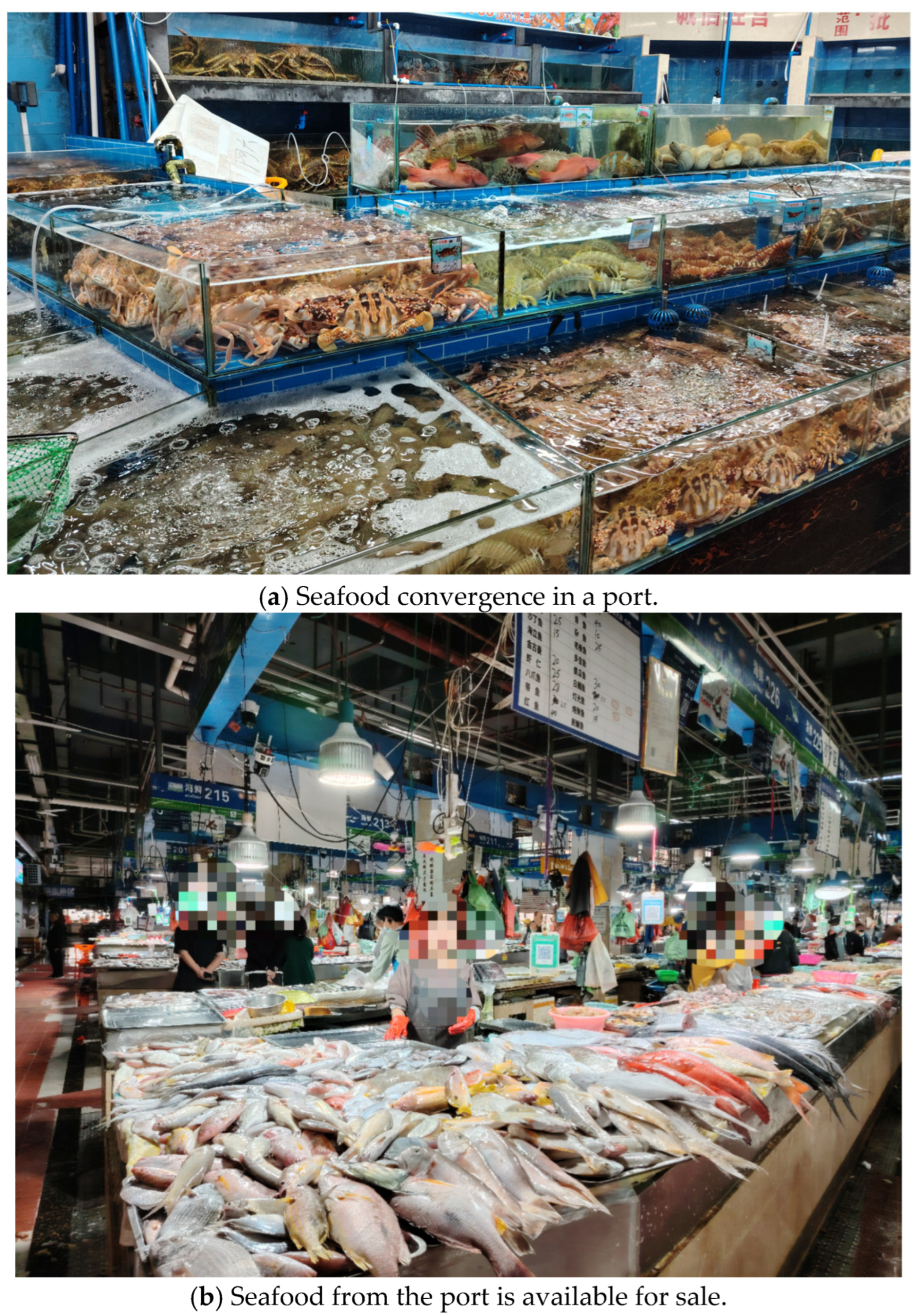
As shown in Figure 1a,b, there is great potential for the growing flow of seafood and zero-carbon transportation in Chinese ports.
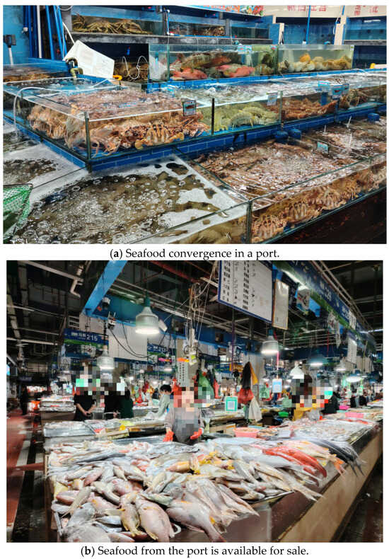
Figure 1.
Growing seafood in China ports with great potential for seafood and zero-carbon transportation flows.
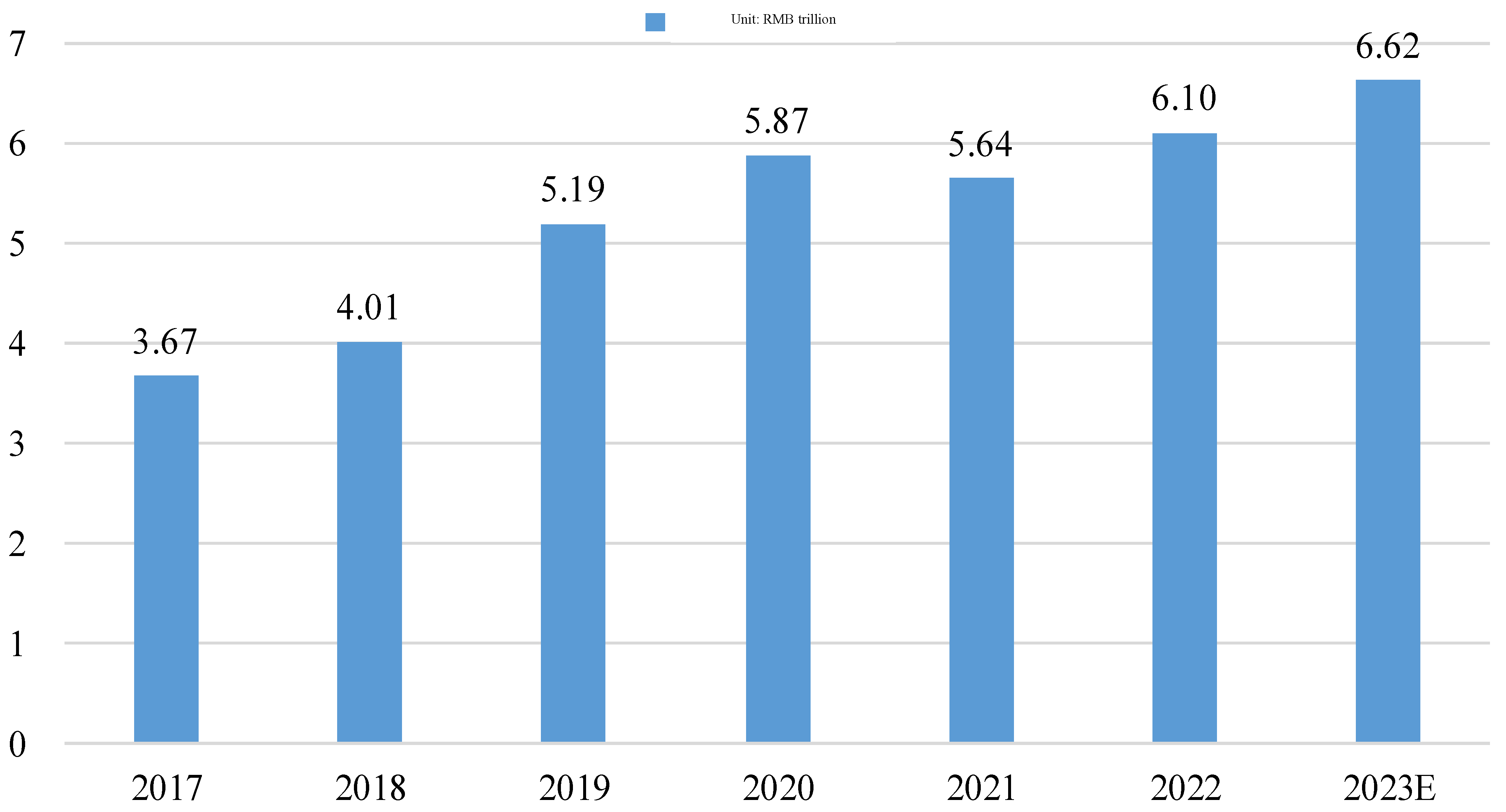
With its rapidly growing port seafood demand and improved infrastructure, China will become the most important contributor to the growth of the Asia–Pacific region, developing into a significant emerging market. China’s logistics industry is booming in emerging markets, not only taking advantage of China’s status as a factory for world goods but also benefiting from rapidly growing domestic demand [4]. The port seafood market size increased from CNY 3.67 trillion in 2017 to CNY 610 million in 2022, with an average annual compound growth rate of 9.21%. 2024E represents the forecast for 2024, which is expected to grow to CNY 6.62 trillion in 2024, as shown in Figure 2 [5].
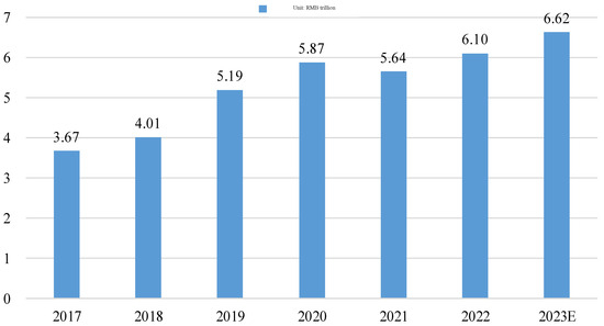
Figure 2.
The size of China’s port seafood market from 2017 to 2024.
In China’s ports, where demand is increasing, the demand for seafood logistics continues to increase. According to relevant statistics, the total demand for seafood logistics in China’s food ports in 2024 will reach 335 million tons, an increase of 37 million tons over 2023 and a year-on-year increase of 10.92%. The demand for the food component of seafood logistics in Chinese ports increased by more than 300% in a decade [6].
The reasonable planning of vehicle routes, improving logistics and distribution efficiency while reducing costs, and meeting consumer needs are the most important issues for port seafood logistics distribution [7]. According to statistics, the number of motor vehicles in China’s cities is growing by more than 10% year by year, and the total number of motor vehicles ranks first in the world. Motor vehicles have gradually become an important part of people’s lives. Traffic congestion has seriously affected the convenience of residents’ travel and life [8]. Considering the traffic congestion situation and ensuring the quality and efficiency of port seafood distribution is a problem that must be considered in port seafood logistics. In recent years, with the continuous progress of science and technology, technologies such as the Internet of Things, big data, and cloud computing have opened a new era of intelligence [9]. Advanced sensing technology and network technology, as well as GPS, Beidou navigation, and other positioning systems, provide technical support for real-time supervision and intelligent vehicle scheduling in the whole logistics chain and continuously strengthen the informatization and intelligent development of the logistics industry [10].
To sum up, traffic congestion is inevitable in daily urban life, and road congestion can affect the driving speed, fuel consumption, and zero-carbon transportation of refrigerated vehicles. For port seafood logistics, energy conservation, and emission reduction are increasingly necessary. On the one hand, port seafood logistics have a great impact on the environment, waste energy, and pollute the environment; on the other hand, the introduction of China’s carbon tax and zero-carbon transportation trading policy will also increase the cost of distribution. Considering the low-carbon and zero-carbon transportation costs in the process of port seafood logistics and distribution is very important for the social and economic benefits of enterprises. Some novel research work has been carried out, such as the need for new energy vehicles for the Internet of Things to establish and maintain reliable optical wireless communication in a network environment [11]. In this paper, the predefined time synchronization problem of coupled neural networks with switching parameters in a new Internet of Things (IoT) energy vehicle system disturbed by Brownian motion is studied [12]. There is a combination of finite-time state feedback and time-varying delay and interference in the network system of new IoT energy vehicles [13]. The research work optimizes the parameters and architecture by synchronizing the genetic algorithm with convolutional neural network blocks to ensure the security of the new energy vehicle network for the Internet of Things [14]. Based on multidimensional quantitative modeling techniques, X. Xiao et al. proposed a computational model to construct effective descriptors by combining metamaterial topology information with additive manufacturing conditions. This descriptor is used as an alternative to the finite element analysis model. It is also possible to build a database of new energy vehicle networks based on the Internet of Things (IoT) to correlate descriptors with mechanical responses obtained from additive manufacturing metamaterial experiments [15]. Y. Qi et al. proposed the complete differential privacy protection of a network security switch LPV system for a new Internet of Things energy vehicle and proposed the complete differential privacy protection of the switching LPV system. The security of the network control system for new IoT energy vehicles lies in the ability to avoid vandalism or accidental interference that affects its normal operation [16]. Zhang C. et al. proposed a unified deep semi-supervised graph learning scheme based on node reweighting and manifold regularization and applied it to the cybersecurity of new energy vehicles for the Internet of Things [17]. Shi Y. et al. proposed an optimal decision based on helicopter–truck–drone collaboration for post-disaster emergency material dispatch, which can be applied to the field of cybersecurity in new energy vehicles for the Internet of Things [18]. The electric vehicle battery disassembly and sorting optimization method based on dynamic Bayesian networks is expected to be applied to the network security of new energy vehicles in the Internet of Things [19].
In 2024, Kaššaj M. et al. discussed how the integration of Industry 4.0 technologies and autonomous vehicles in smart city infrastructure will significantly improve traffic efficiency, resource utilization, and overall urban sustainability. The pros and cons of such an integration were examined, emphasizing the benefits in terms of reduced environmental impact and improved quality of life for citizens on the one hand and the various ethical, legal, and social issues that such an integration may raise on the other. Several approaches were used, namely analytical, synthetic, comparative, and historical interpretation. The final discussion highlighted the benefits and challenges that such an integration faces and that must be addressed in order for it to be successful. It can be concluded that the synergistic potential of autonomous vehicles and Industry 4.0 in smart city infrastructure is enormous and that such an integration offers promising solutions for improving traffic efficiency, energy management, and overall urban sustainability [20]. Recently, Kateryna Nekit. et al. analyzed the concept and legal issues of the Internet of Things to explore whether the existing legal framework is suitable for dealing with this new phenomenon. They examined the body of legal issues in the field of the Internet of Things and how to solve them. They also considered how to deal with damages caused by the Internet of Things. They considered the conditions for compensation for damages caused by IoT devices. The need for self-regulation in the field of the Internet of Things was emphasized to ensure information security and prevent damages caused by the Internet of Things. This would be possible if technology companies and civil society work closely together. Such an approach would minimize government intervention in this field, which would contribute to the rapid development of innovative technologies [21]. Gonçalves M. et al. comprehensively explored the process of creating a reliable business intelligence solution by analyzing the container delivery and pickup service processes in one of the largest maritime container ports in Portugal using the CRISP-DM approach [22].
Based on the research of the above studies, this research analyzes and studies traffic congestion and zero-carbon traffic in the process of seafood logistics distribution in urban ports, constructs a multi-objective optimization model, and conducts simulation analysis. Firstly, we calculate the driving time of the vehicle and build a multi-objective optimization model. The road is divided and the traffic congestion index is used to find the time when the vehicle arrives at each customer point and the travel time. We analyze the costs in the distribution process and establish a multi-objective optimization mathematical model with the goal of minimizing the distribution cost of port seafood logistics and the minimum cost of zero-carbon transportation. Secondly, the traffic congestion index, carbon trading price, and temperature difference between the inside and outside of the refrigerated truck are adjusted, respectively, and the distribution time and distribution cost are positively correlated with the congestion state of the road. With the increase of carbon trading prices, the total cost of port seafood logistics and distribution is generally on the rise.
The rest of this research is organized as follows. We investigate the description of the model of zero-carbon transportation and the multi-objective optimization of port seafood in Section 2. We propose the construction of a multi-objective optimization mathematical model of port seafood logistics in Section 3. Simulation results and analysis of actual case studies are conducted in Section 4. Sensitivity analysis and experimental verification are carried out in Section 5. Finally, concluding remarks and future directions are given in Section 6.
2. Description of Model of Zero-Carbon Transportation and Multi-Objective Optimization of Port Seafood
The optimization of a multi-objective port seafood logistics path considering traffic congestion and zero-carbon traffic is divided into three aspects: The first is port seafood logistics, including the definition, characteristics, and operation mode of port seafood logistics. The second is the analysis of vehicle routing problems considering traffic congestion and zero-carbon traffic, including vehicle routing problems; time-dependent function analysis considering traffic congestion; zero-carbon traffic volume and fuel consumption solution analysis; and carbon tax and carbon trading systems. The third is the multi-objective optimization problem, including the definition of the multi-objective optimization problem and the general solution algorithm.
2.1. Port Seafood Logistics Description
The Chinese standard “Logistics Terminology” (GB/T18354-2021) [23], which was published in August 2021 and implemented in December 2021, defines port seafood as logistics technology and organizational systems that keep goods, from production to consumption, at the required temperature according to the characteristics of the goods. For port seafood logistics, the national standard “Port Seafood Logistics Classification and Basic Requirements” defines it as using refrigeration technology as a means and freezing technology as the basis for keeping port seafood items in a constant-temperature environment from production to circulation, sales, customers, and other links so as to ensure the quality of port seafood items and reduce the loss of port seafood items. The port seafood logistics studied in this research refer to the logistics stage of port seafood products from the refrigerated distribution center to the point of demand.
The service object of port seafood logistics has the characteristics of fragility and perishability, and port seafood logistics are more special than ordinary logistics, which are mainly divided into the following points:
- (1)
- High cost and high risk
Due to the special nature of port seafood products, it is necessary to keep the whole chain at a low temperature. It is necessary to use equipment such as cold storage and refrigerated trucks that can maintain low temperatures, and the personnel investment cost is higher and the total investment cost is high. In addition, port seafood products are prone to damage and deterioration due to their particularity, resulting in a greater risk of cargo loss.
- (2)
- High requirements for temperature control
The main difference between port seafood logistics and other types of logistics is that port seafood logistics must strictly control the low temperature of goods during transportation. In order to achieve this purpose, the whole process of port seafood logistics from the processing to the storage, distribution, and sales of goods must have very strict refrigeration and low-temperature control for the goods, and different products may have different temperature requirements, and the temperature needs to be reasonably regulated to ensure that the loss of products is minimized.
2.2. The Mode of Operation of Port Seafood Logistics
According to the current situation of China’s port seafood and agricultural products’ port seafood logistics, the main operation modes of port seafood and agricultural products’ port seafood logistics are divided into the following according to the core of the overall logistics chain:
- (1)
- The operation mode with processing enterprises as the core
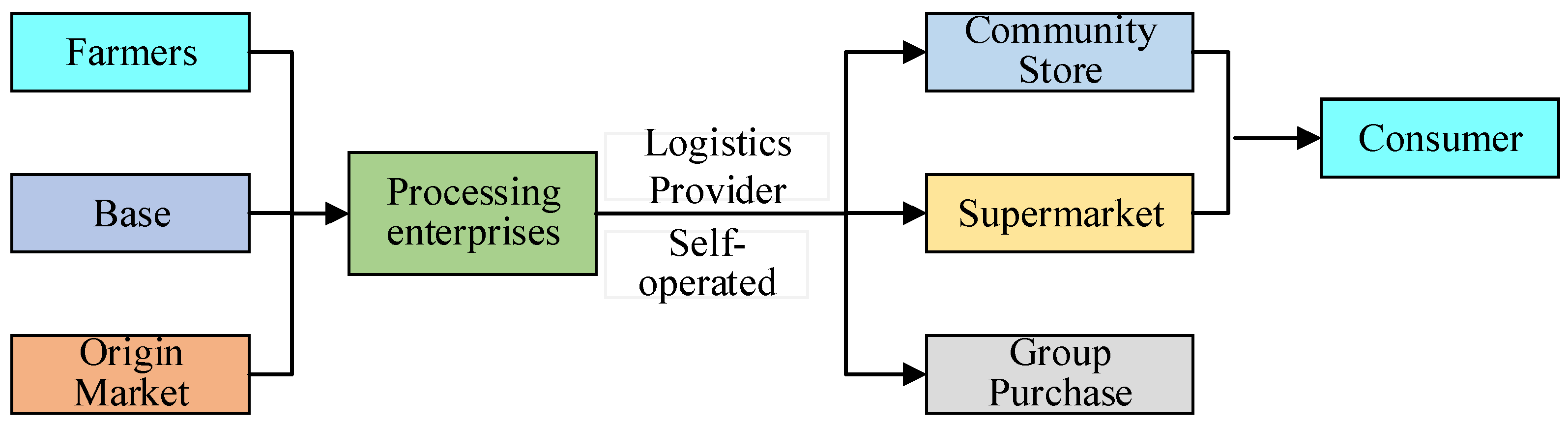
The processing of port seafood products is the foundation of the development of agricultural industrialization and a key link in the port seafood industry chain. In this mode, large-scale port seafood and agricultural product processing enterprises, as core enterprises, can be self-sufficient, self-controlled, or cooperative stores or can directly enter supermarkets and control commercial terminals, as shown in Figure 3.
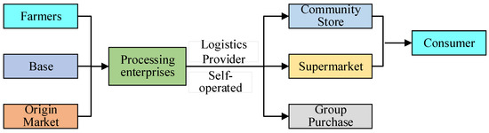
Figure 3.
The operation mode with processing enterprises as the core.
- (2)
- Wholesalers as the core mode of operation
Under this model, the core enterprise of the food supply chain is the wholesale of seafood and agricultural products at the port. Wholesalers link the production, distribution, and wholesale of agricultural products forward and link the circulation and retail links of products backward, as shown in Figure 4.
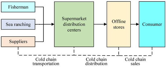
Figure 4.
The supermarket chain is the core mode of operation.
- (3)
- The operation mode with supermarket chains as the core
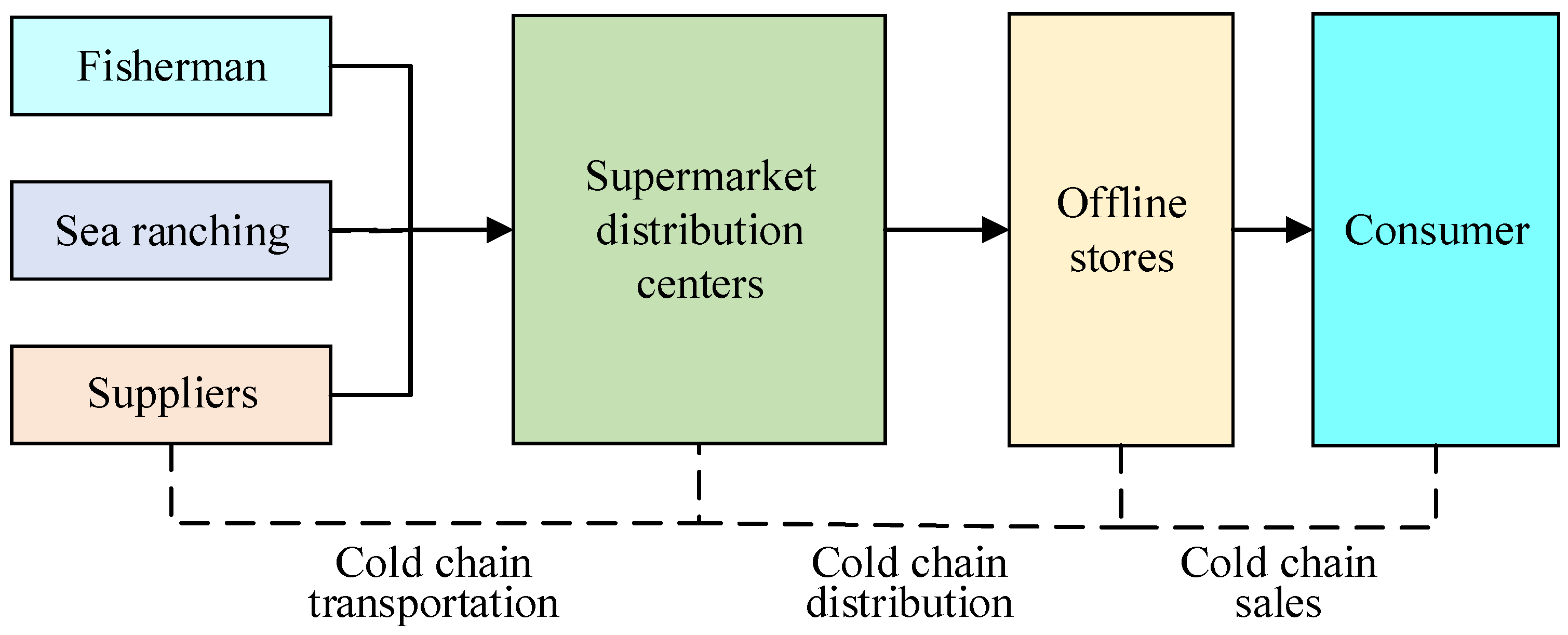
Compared to traditional farmers’ markets, large supermarket chains have a clean and comfortable shopping environment; the open, transparent, convenient, and fast one-stop shopping method can meet all the daily needs of residents and is more suitable for the fast-paced pace of contemporary life. Large supermarket chains generally have a more complete and excellent port seafood logistics supply system; relying on the demand for port seafood and agricultural products, they cooperate with suppliers, that is, fishermen or bases, and distribute port seafood and agricultural products to various offline stores of downstream supermarket chains with the help of specialized logistics partners, as shown in Figure 5. Port seafood supermarkets can better trace the source of port seafood products and ensure the quality and freshness of port seafood products, and more and more residents are more willing to go to large supermarket chains to buy port seafood products.

Figure 5.
Manlandraki time-dependent function.
Table 1 describes VRPs from the perspectives of the number of distribution centers, the number of objective functions, the type of vehicles, the type of time window, and the information status.

Table 1.
Classification of vehicle routing problems.
2.3. Analysis of the Time-Dependent Function Considering Traffic Congestion
Traffic congestion has become a daily phenomenon in urban areas due to the growing volume of port logistics traffic and the limited capacity of road networks. Traffic congestion causes significant variations in vehicle travel times and speeds on urban roads, especially during the morning and evening rush hours. In real life, traffic conditions change throughout the day, and the travel time and speed of vehicles in the transportation network change depending on the time of day. In general, the time-dependent function is used to describe it, and the time-dependent function is established under ideal conditions. There are two commonly used time-dependent functions.
- (1)
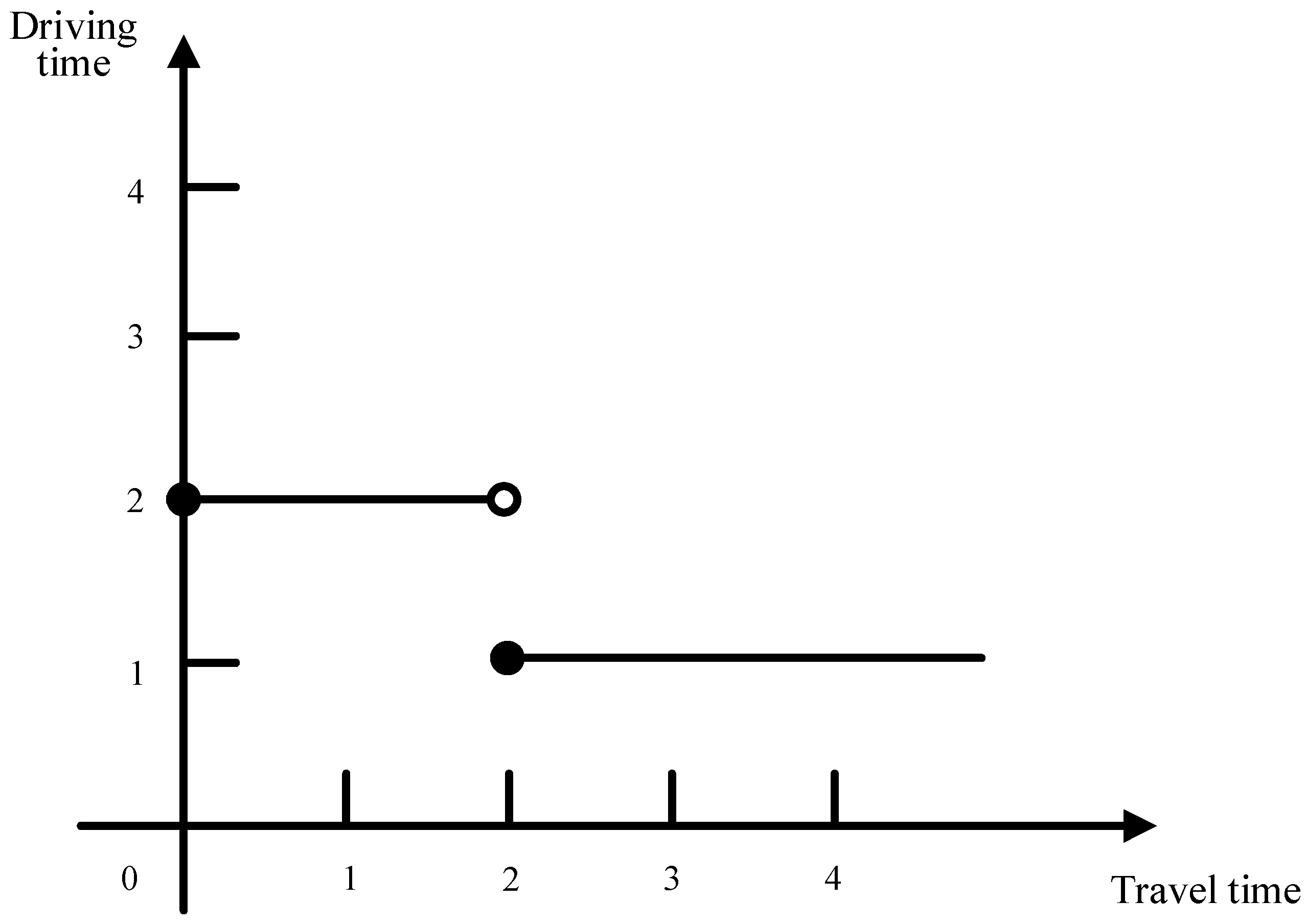
- Manlandraki time-dependent function
The Manlandraki time-dependent function indicates that the travel time of a vehicle between two points is related to the departure time of the vehicle. The time of day is segmented, and the travel time is described as a stepped function of the departure time, as shown in Figure 5. However, the model does not satisfy the First-In-First-Out (FIFO) rule, i.e., for the same stretch of route (), the vehicle that departs first does not necessarily arrive first. For example, if vehicle 1 departs at the time of 1.5, and the vehicle travel time is 2 according to the Manlandraki time-dependence function, then the vehicle arrives at the time of arrival 3.5. Vehicle 2 departs at the time 2, and according to the Manlandraki time-dependence function with the vehicle travel time 1, the vehicle arrival time is 3, which does not satisfy the FIFO rule.
The Ichoua time-dependent function considers the phenomenon that the speed of the vehicle changes across the time domain during driving. And, in line with the FIFO principle, it is more in line with the traffic congestion of the actual road network of the city. In this research, the driving time of the vehicle is calculated on the basis of the Ichoua time-dependent function.
2.4. Zero-Carbon Traffic Volume and Fuel Consumption Solution Analysis
With the rapid development of the global economy, the problem of global warming caused by carbon transportation is becoming more and more prominent, threatening the natural ecosystem and human survival, and scholars are paying more and more attention to the problem of zero-carbon transportation in the problem of vehicle paths. The zero-carbon traffic generated by a fuel vehicle is linearly related to fuel consumption, as shown in Equation (1):
In the equation, CE represents the zero-carbon traffic generated by the vehicle during driving, represents the emissions per unit of fuel consumption, and represents the fuel consumption of the vehicle. Most scholars use the fuel consumption of vehicles to calculate the amount of low-carbon traffic. There are two main types of models for solving the fuel consumption of vehicles:
- (1)
- Instantaneous fuel consumption calculation model
The unit fuel consumption of a vehicle is solved using the vehicle traction force, load, and fuel consumption rate, as in Equations (2) and (3):
where in is fuel consumption per unit of time; represents vehicle traction; is the fuel consumption of the vehicle when there is no load; denotes fuel consumption per unit of energy; represents fuel consumption per unit of energy acceleration; indicates the weight of the vehicle when unloaded; denotes acceleration; denotes speed; and represent rolling resistance and air resistance; denotes acceleration due to gravity; and is the percentage grade.
The total fuel consumption of the vehicle for time can be expressed as Equation (4):
2.5. Carbon Tax and Carbon Trading System
At present, the commonly used carbon emission reduction strategies are mainly carbon tax and carbon trading. A carbon tax is a tax levied on non-zero-carbon transportation to reduce the volume of non-zero-carbon transportation. The full name of carbon trading is “zero-carbon transportation rights trading”. The Kyoto Protocol adopted by the United Nations Intergovernmental Panel on Climate Change in December 1997 uses the market mechanism as a new way to solve the problem of reducing carbon dioxide greenhouse gas emissions; that is, the zero-carbon dioxide transportation allowance is traded as a commodity, which is called carbon trading, and the corresponding market is called the carbon market, and the carbon trading process is shown in Figure 6.
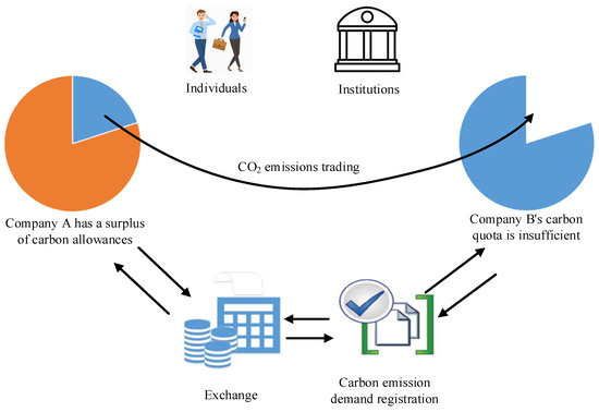
Figure 6.
Schematic diagram of carbon trading.
2.6. Model Description of Multi-Objective Optimization Problem
There are two main types of methods for solving multi-objective problems: the first method is the linear weighting method, which transforms the multi-objective method into a single-objective optimization problem through the method of weight allocation and solves it by using various single-objective optimization methods. Another ideal method is to use a multi-objective evolutionary algorithm to generate a solution set to solve this problem, and the obtained solution set is located on a Pareto front.
If all objectives are minimum, the multi-objective optimization problem can be described as Equations (5) and (6):
Here are the decision variables taken from the -dimensional space ; is the -dimensional objective function; are inequality constraints; are equation constraints. For multi-objective optimization problems, the optimal solution can achieve the best results of multiple objectives. The solution to the multi-objective optimization problem is a set of Pareto solution schemes.
Definition 1.
(Pareto domination) Suppose that and are the two solutions in MOP(1). If and only if Pareto-dominates (denoted as < ), then for all , and at least one satisfies .
Definition 2.
(Pareto optimal solution) If there is no solution, Pareto-dominates ; the solution is called the Pareto optimal solution.
Definition 3.
(Pareto front) The set of vectors corresponding to the Pareto optimal set in the target space is called the Pareto front.
3. Constructing a Multi-Objective Optimization Mathematical Model of Port Seafood Logistics
Considering the traffic congestion faced by port seafood delivery vehicles during driving, the traffic congestion index is used to express the traffic congestion degree in different time periods and calculate the vehicle speed with time. We divide the road section and calculate the travel time of a vehicle. The distribution cost and zero-carbon transportation of port seafood logistics are comprehensively analyzed, and a multi-objective optimization model is proposed with the goal of minimizing distribution cost and zero-carbon transportation cost.
3.1. Study Description and Drive Time Analysis
Aiming at the port seafood distribution process of port seafood products in supermarket chains, the optimization of a multi-objective port seafood logistics path considering traffic congestion and zero-carbon traffic is studied. A port seafood logistics distribution center has homogeneous refrigerated trucks that need to distribute port seafood products to supermarket chains. Information such as the geographical location and demand quantity of each supermarket chain, as well as the time window, are known. All vehicles depart from the distribution center and return to the distribution center as soon as the delivery task is completed. Traffic congestion in the road network changes over time, affecting the speed at which vehicles can travel. We comprehensively consider the various distribution costs and zero-carbon transportation costs generated in the process of vehicle distribution and construct a multi-objective optimization model. On the basis of considering traffic congestion and zero-carbon traffic, the multi-objective vehicle route optimization problem with time window is solved, and the optimal vehicle scheduling scheme and route planning are finally obtained.
This article obtained real-time vehicle location, travel data, vehicle lanes, and other road traffic-related data through Baidu map-2025 software. The higher the traffic congestion index is, the higher the congestion level is. When the road is completely clear, we assume that the vehicle speed is , the congestion index of each road section is , and the vehicle travel speed in the sub-road section is constant. In the case of time-varying networks, the congestion period of urban roads is known due to the prediction of big data. Vehicles may be in the same lane partly in the open and partly in the congested period. We divide the road section and solve for the actual travel time of the vehicle. The specific steps are as follows:
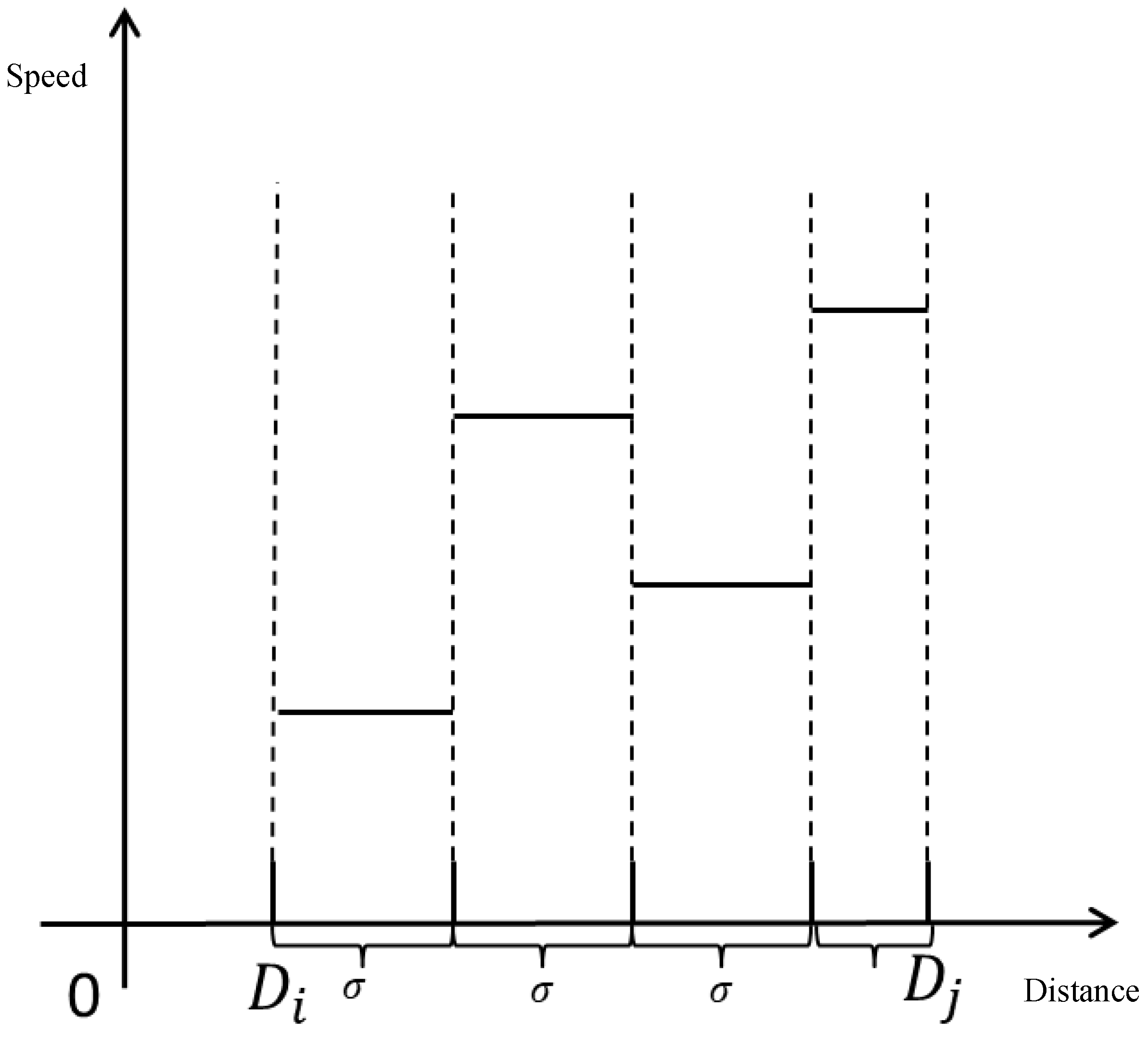
Step I: Divide the road segments. Specify the distance between customer point and customer point in . According to , they are divided into (rounded up) sub-sections, and the first sub-sections are all . The -th sub-section is .
Step II: Calculate the travel time for each sub-segment. The time point at which the car leaves customer point is the starting time of the vehicle section ; then, the traffic congestion index is . The travel time for a subsegment with a distance of is = . The driving time of the -th sub-section is , and the driving time of each sub-section is shown in Figure 7. The start time of the second sub-segment is and the start of the third sub-segment is , …. The beginning moment of entering the -th sub-section is ;
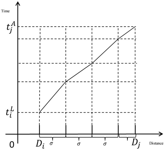
Figure 7.
Travel time for each sub-segment.
Step III: Calculate the total travel time of the vehicle in the road section . The travel time of vehicle on the road can be expressed as Equation (7):
The moment of arrival at customer point is Equation (8):
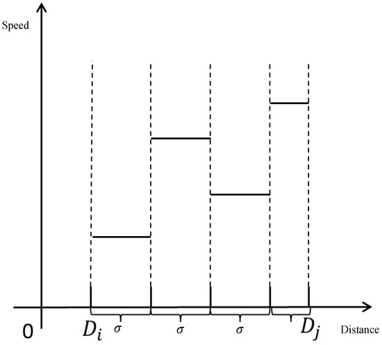
Figure 8.
The driving speed of each sub-section.
3.2. Multi-Objective Optimization Model Construction
3.2.1. Distribution Cost Analysis
We conduct optimization studies on the basis of the company’s existing logistics facilities. The enterprise already has a batch of homogeneous refrigerated vehicles and the distribution center has been built, regardless of the vehicle purchase cost, distribution center construction cost, and distribution center use cost. Port seafood products are perishable, have a certain loss rate, and need to be stored and transported under low-temperature conditions. The port seafood logistics distribution costs considered in this article include the following.
- (1)
- The cost of vehicle use
After the vehicle departs from the distribution center, it must pay a certain cost, , for vehicle use, including the driver’s salary, vehicle wear and tear, and maintenance costs. The cost of vehicle usage is usually constant, so the total cost of the vehicle usage can be expressed as Equation (9):
- (2)
- Refrigeration costs
In the distribution process, the refrigeration cost of a refrigerated truck consists of two parts. They are the refrigeration costs incurred during driving and the refrigeration costs incurred during unloading. During driving, due to the particularity of the product, it is necessary to maintain a low temperature. Refrigeration units need to work continuously, incurring a certain amount of refrigeration costs. Since all the goods are unloaded, in order to save energy and reduce emissions, the vehicle finally stops the refrigeration in the box during the return journey. The cooling costs incurred during driving can be expressed as in Equation (10):
is the heat load generated by the refrigeration facility during the driving of the k-th refrigerated truck: . Here, is the depreciation rate of the vehicle. The constant is the heat transfer rate. is the heat transfer area of the refrigerated truck; the unit is . is the temperature difference between the inside and outside of the refrigerated compartment; the unit is . is the unit refrigeration cost. is a 0–1 variable, and means that the vehicle returns to the distribution center 0 from customer point .
When the vehicle arrives at the customer’s unloading point and the reefer is opened, the hot air outside will convect with the cold air inside the reefer. As a result, the cooling and heating loads of the cooling system enter the vehicle, resulting in cooling costs. The refrigeration cost incurred by the refrigerated truck in unloading can be expressed as in Equation (11):
where in is the heat load generated by the refrigeration facility during the unloading of the -th refrigerated vehicle: . is the frequency coefficient for opening the refrigerator; the specific values are shown in Table 2. is the volume of the compartment of the refrigerated vehicle; is the temperature difference between the inside and outside of the refrigerated warehouse; and is a 0~1 variable.
Table 2.
Frequency coefficient of door opening.
Using the same type of refrigerated vehicle, the volume of the refrigerated compartment and the temperature in the compartment are the same. The door-opening frequency of each refrigerated truck is taken as the number 0.4.
The cooling cost of a vehicle can be expressed as Equation (12):
- (3)
- Fuel costs
Consider that the cost of vehicle fuel consumption refers to the cost of fuel consumed by the engine while the vehicle is driving. Using the fuel consumption calculation model based on the load capacity, the fuel consumption (FC) of the vehicle can be expressed as Equation (13) from Equation (12):
The fuel cost of a refrigerated vehicle can be expressed as Equation (14):
- (4)
- Cost of cargo damage
Due to the perishable characteristics of port seafood products, port seafood products will receive a certain degree of damage during transportation and unloading. For example, the oxidation of wounds may occur in port seafood products after a collision during transportation and handling. As a result, the product will rot and microorganisms will multiply on the seafood products in the port, resulting in mold, fermentation, and deterioration, affecting the quality of the product. The cost of damage in the distribution process includes two aspects: there will be a certain cost of damage during transportation, and there will also be a certain cost of damage during the unloading process. The spoilage degree function of port seafood is ; is the starting weight of the port seafood, and is the fresh spoilage coefficient of the port seafood.
The cost of loss incurred during transportation, , is expressed as Equation (15):
The cost of loss incurred during unloading, , is Equation (16):
The total cost of damage, , is expressed as Equation (17):
- (5)
- Time penalty cost
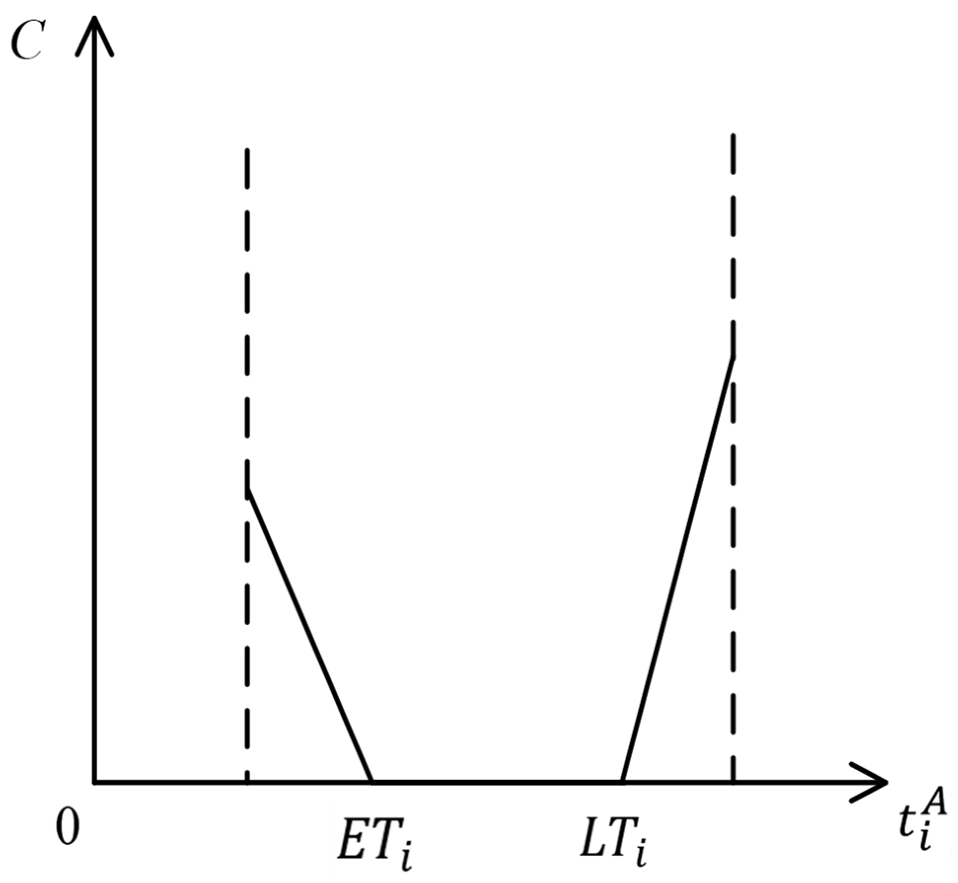
In the actual logistics distribution, the customer will set the arrival time of the delivery service according to their own needs. The distribution center is obliged to arrive and complete the delivery service within the time frame specified by the customer as well as possible in order to improve the efficiency of completing the delivery task. In the actual distribution process, due to uncontrollable risk factors such as changes in traffic and weather conditions, the arrival time of logistics and distribution vehicles will be affected, and the goods may even not be delivered on time. The actual vehicle arrival time () penalty amount is required to be paid in advance of or beyond the range of the customer’s specified time window , with being the earliest time of service allowed and being the latest time of arrival allowed. Figure 9 shows the penalty cost of port seafood logistics delivery time constrained by a soft time window.

Figure 9.
Soft time windows constrain delivery time penalty costs.
The total time penalty cost can be expressed as in Equation (18):
3.2.2. Analysis of Zero-Carbon and Low-Carbon Transportation Costs
The goal of green logistics is to adopt zero-carbon, low-carbon, and clean production operations. This involves implementing the concept of sustainable development and reducing carbon dioxide and carbon dioxide-based transportation in the logistics process. Based on the development concept of green logistics, the traffic volume of zero-carbon transportation is combined with the cost of optimizing the distribution route of seafood logistics in the port. The zero-carbon transportation costs considered in this research mainly include two parts: the direct zero-carbon transportation costs generated by the diesel fuel consumed by the power consumption of vehicles and the indirect zero-carbon transportation costs generated by the diesel fuel consumed by the electrical energy used to maintain the temperature of refrigerated compartments.
The zero-carbon and low-carbon traffic volume of vehicles from customer point to with a load capacity of can be expressed as Equation (19):
The amount of zero-carbon and low-carbon traffic generated by vehicles from customer point to due to refrigeration can be expressed as Equation (20):
where in is the emission factor when the vehicle is driving, and is the emission factor of the vehicle refrigeration unit mass and the unit distance of the goods. Carbon trading is used to calculate the cost of zero-carbon and low-carbon transportation. is the carbon trading price, and is the zero-carbon and low-carbon transportation quota for enterprises. The total zero-carbon transportation cost in the process of vehicle distribution is Equation (21):
3.2.3. Logistics Model Construction
In order to solve the problem of multi-objective port seafood logistics path optimization considering traffic congestion and zero-carbon traffic, a multi-objective optimization model is proposed with the goal of minimizing distribution cost and zero-carbon transportation cost, as Equations (22) and (23).
Constraints:
Equation (24) indicates that each customer is served by only one vehicle. Equation (25) represents the capability constraints of the vehicle. The customer’s demand is less than or equal to the maximum load of the vehicle. Equation (26) indicates that the start node and end node of each vehicle are distribution centers. Equation (27) indicates that the vehicle must leave after completing the service. Equation (28) indicates that the amount of load shed after customer point completes the service is equal to the amount demanded by customer . Equation (29) indicates that the number of customers served by the distribution center is . Equation (30) excludes the existence of idle carbon allowances and ensures that enterprises make full use of the carbon trading mechanism.
3.2.4. Improved NSGA-II Algorithm Steps
The specific steps of the improved NSGA-II algorithm are as follows:
Step 1. Initialize the population, randomly generate a population, , with the number of individuals N; 0.
Step 2. Carry out the non-dominant ranking of the initial parent population, and calculate the individual crowding considering variance.
Step 3. The binary championship selects the outstanding individuals in the population , crosses and mutates the outstanding individuals, and produces of offspring populations.
Step 4. Combine and into to perform a fast non-dominant ranking of . Calculate the crowding degree, and use the elite strategy to select the top individuals to form the parent population, ; .
Step 5. Randomly select some outstanding individuals in the new parent population for a simulated annealing operation for local search. The population number is , and the parameters are initialized.
Step 6. The neighborhood search generates a new individual, , and calculates the corresponding and .
Step 7. If and , accept the new solution as the current solution. Otherwise, according to the improved metropolis, calculate and judge whether to accept the solution; that is, randomly generate the probability value . If , the new solution is accepted; otherwise, it remains unchanged.
Step 8. If the minimum temperature is reached, terminate the algorithm, retain the current solution, and go to Step 9; otherwise update the temperature, and the algorithm will go to Step 6.
Step 9. Judge whether the population number has reached . If this is satisfied, stop the local search to generate an alien population; otherwise, go to Step 6.
Step 10. Merge the alien population with the new population .
Step 11. Conduct the elite selection of merged populations to generate a new generation of populations.
Step 12. Determine whether the maximum number of iterations is reached. If it is reached, stop the operation and output the result; otherwise, go to Step 2.
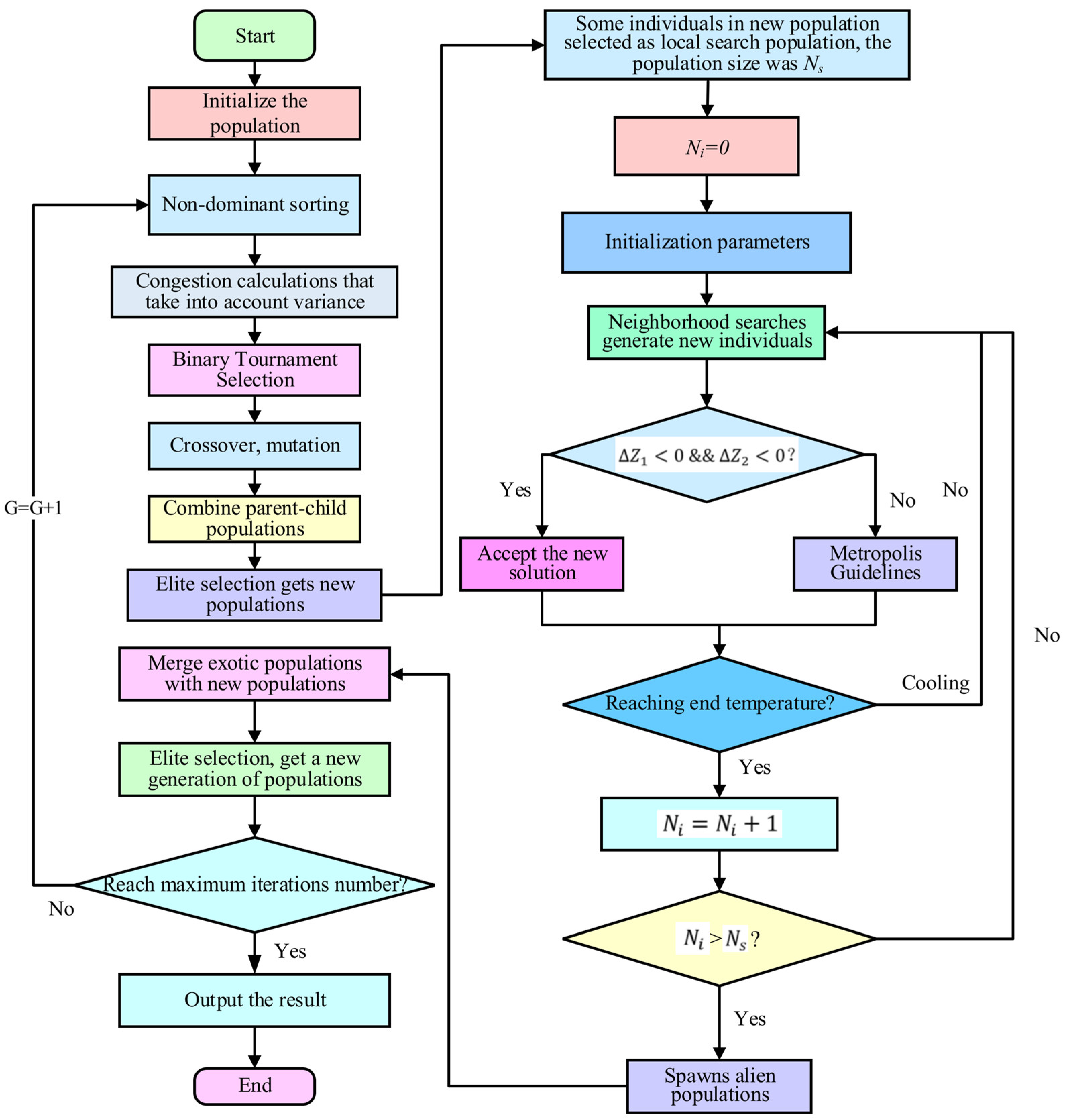
The specific flow of the improved NSGA-II algorithm is shown in Figure 10.
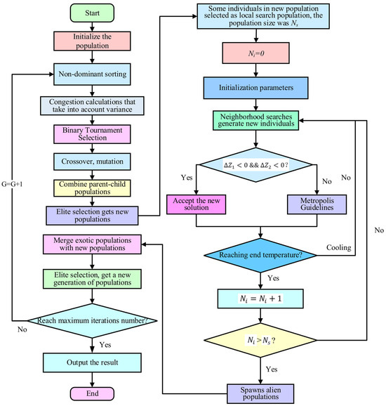
Figure 10.
Flowchart of improved NSGA-II algorithm.
4. Actual Case Analysis
4.1. Case Description
Zero-carbon transportation supply chain company A is a logistics company located in Shenzhen, mainly providing port seafood distribution services. Company A supplies port seafood products such as kelp, marine fish, sea crabs, shrimp, and seashells to some supermarkets in the city from its existing distribution center. It focuses on urban distribution services, its own vehicles, sufficient capacity, and the use seafood trucks in the whole port. It provides customers with same-day delivery port seafood logistics and distribution services in the same city. The distribution center has sufficient goods, and refrigerated trucks are transported according to the order address provided by the customer. The transportation equipment and carrying operation are in line with industry norms, and the goods are completely directed to be delivered through a point-to-multi-point manner, avoiding transit links. Company A has one distribution center; the location is known and has been built. Company A’s refrigerated trucks are equipped with sensing equipment, GPS, and temperature monitoring systems, allowing them to be monitored throughout the process. These trucks must report their whereabouts in real time and monitor the temperature inside the refrigerated trucks in real time. At the same time, the company can provide customers with value-added services such as temperature data, document recovery, quotation, and so on.
The logistics distribution path selection of company A in the zero-carbon transportation supply chain is mainly based on the driver’s requirements according to the location and time window of the customers served. Based on past driving experience, the driving time of the vehicle is estimated based on the speed of the vehicle when the road is completely clear, and the delivery route of the day is determined. The distribution route planning is not scientific, and customers often complain about problems such as untimely delivery and large damage to seafood products in the port. The port seafood logistics path of company A, a zero-carbon transportation supply chain that joins the carbon trading market, is planned. Traffic congestion is considered in order to meet the basic needs of customers. Enterprise costs and zero-carbon transportation are reduced, contributing to China’s green and sustainable development.
4.2. Basic Transportation Data
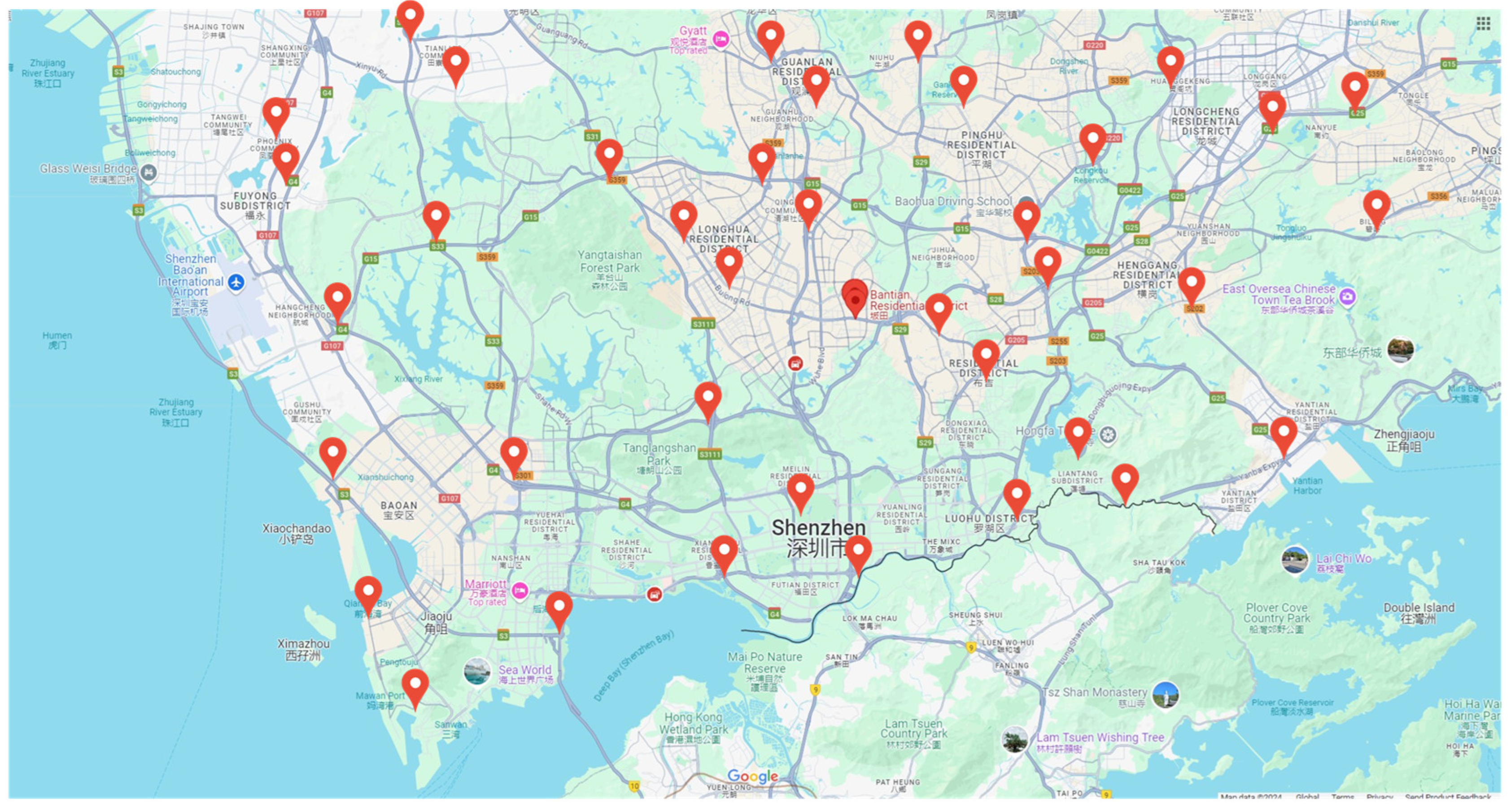
In this section, we describe how the distribution task information of the Shenzhen-based zero-carbon transportation supply chain company A on a certain day was used to plan the path. We took one distribution center and order data from 20 customer points as a test case; the path was planned, and the specific location distribution is shown in Figure 11.
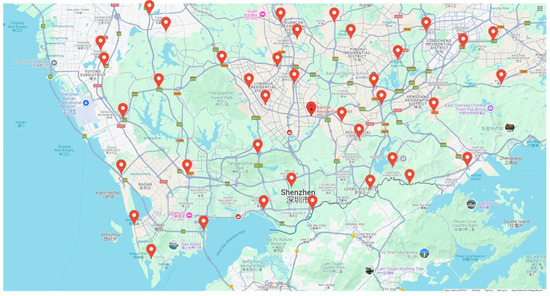
Figure 11.
Distribution map of specific location of each node in Shenzhen.
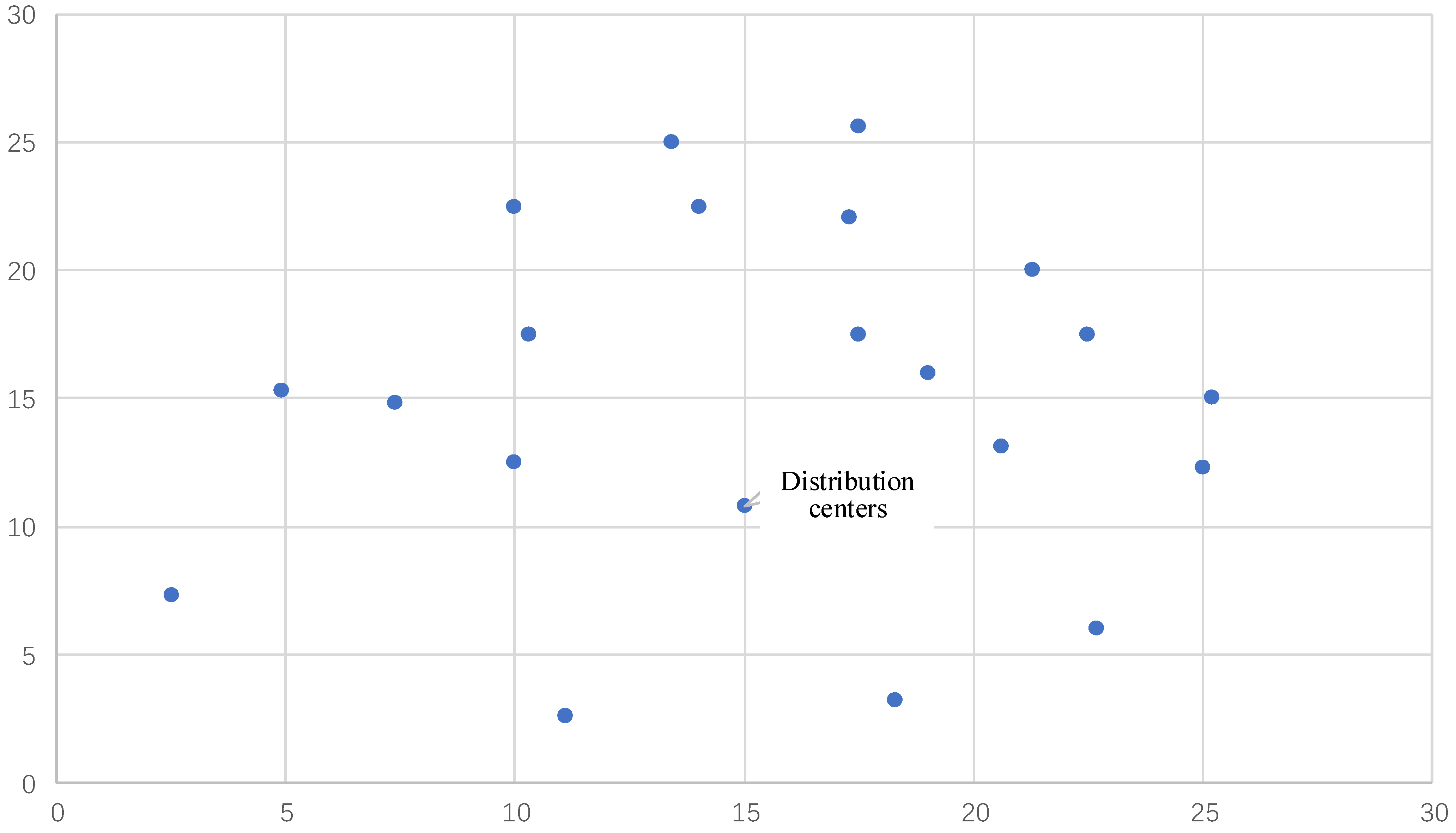
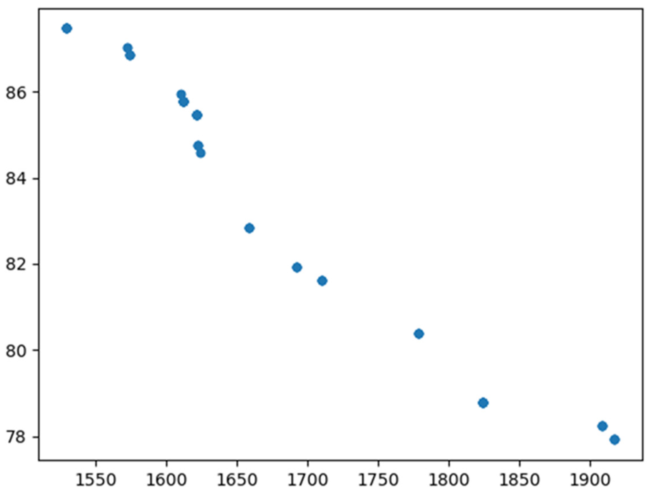
Table 3 shows the demand, time window, and service time of the customer points, where 0 represents the distribution center and 1–20 represent the customer points. We set the position of the circle center in the lower left corner of Figure 10 as the coordinate origin (0,0) and converted the location of company A and each customer point in the zero-carbon transportation supply chain into a planar Cartesian coordinate system. The location of the processed customer point is shown in Figure 12.
Table 3.
Customer information.
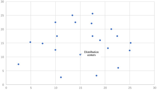
Figure 12.
The location of the distribution center and the customers’ plane coordinates.
According to the historical data analysis and prediction of Baidu map, the morning peak time on 10 May 2024 was 7:00~9:00, as shown in Figure 13. The traffic congestion index for each time period is shown in Table 4. We set the corporate carbon quota and studied the distribution demand of 6:00~12:00 a.m. on 30 May 2024 according to the special distribution requirements of seafood products in the port. Assuming that the vehicle speed was 60 km/h when the road was completely clear, 6:00 was set to 0 from 6:00 a.m.
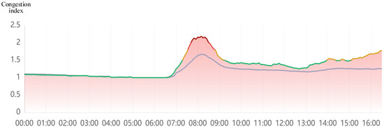
Figure 13.
Traffic congestion prediction(Red: congestion; Green: unblocked; Blue: General).
Table 4.
The traffic congestion index for each time period, .
.
4.3. Solving of Single-Objective Optimization Models Without Considering Zero-Carbon Transportation
In order to test the superiority of the multi-objective optimization model proposed in this research, we consider both distribution cost and zero-carbon transportation cost. A single-objective optimization model with the goal of minimizing distribution cost is established, and the resulting single-objective model is Equation (31):
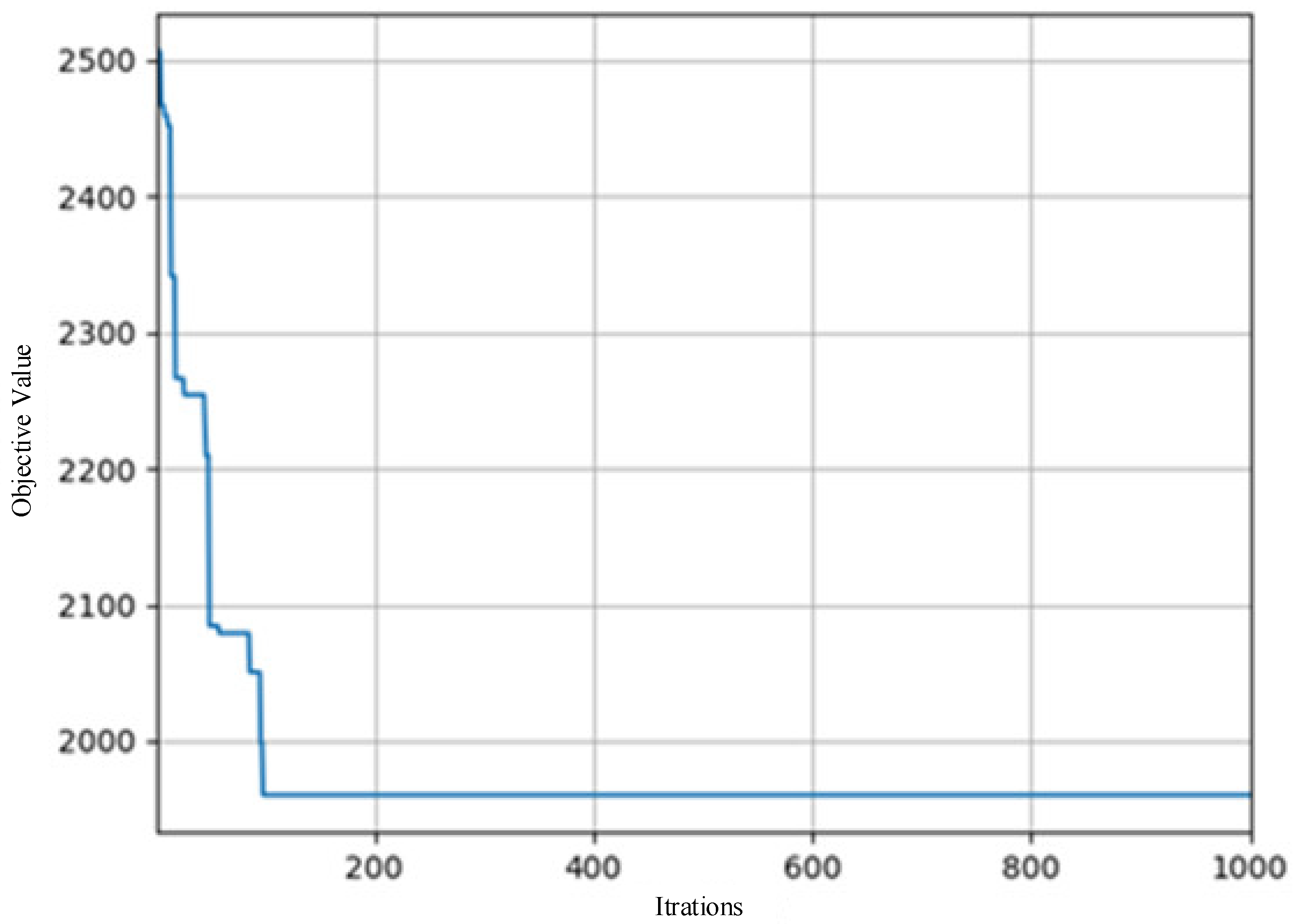
The genetic algorithm was used to solve the example, and parameters such as the population number, crossover, and mutation probability were consistent with those of the improved NSGA-II algorithm. Figure 14 shows the convergence curve of the algorithm. The algorithm could achieve convergence within 200 generations of iterations and obtain the optimal solution.
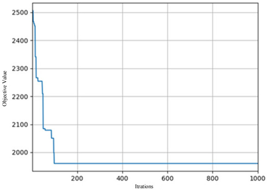
Figure 14.
Convergence curve.
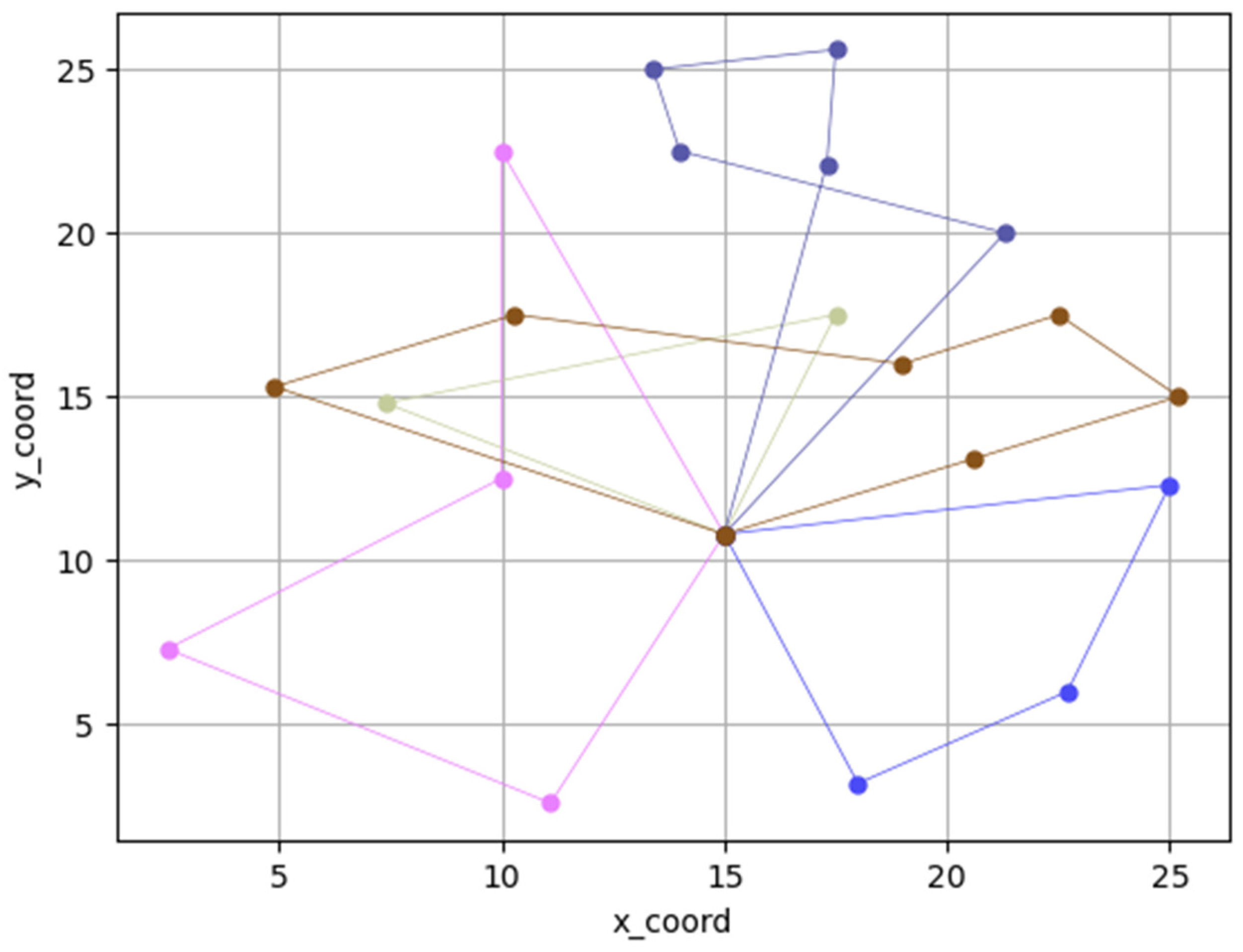
Without considering the zero-carbon traffic volume, the single-objective optimization model was used to solve the example, and the distribution cost was CNY 1587.74. The actual zero-carbon traffic volume was 256.42 kg, and a total of five vehicles were used for delivery. Figure 15 shows the path optimization scheme.
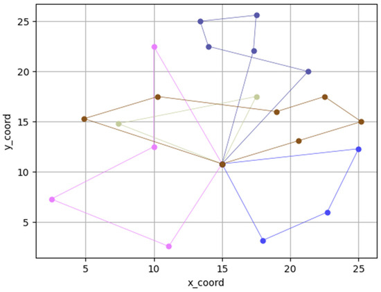
Figure 15.
Optimal vehicle paths (different colors represent 5 vehicles for delivery route optimization).
4.4. Solving of Multi-Objective Optimization Models Considering Zero-Carbon Transportation
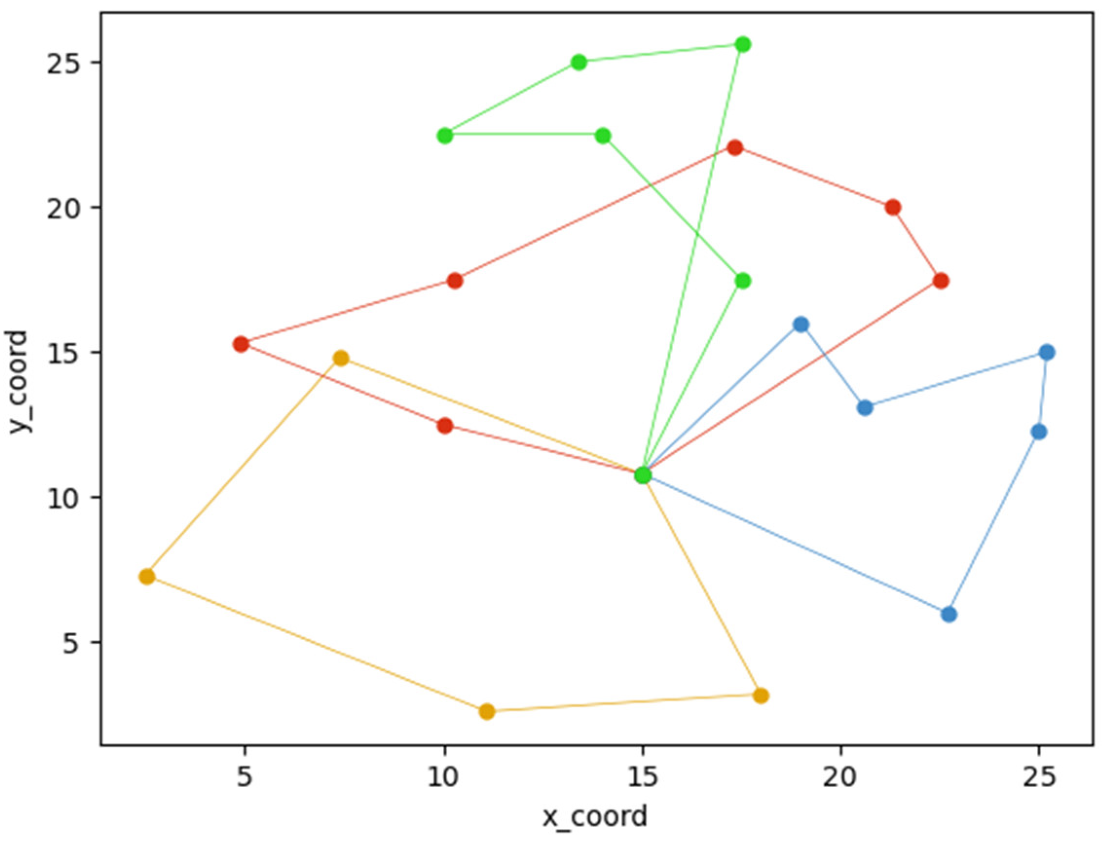
The improved NSGA-II algorithm was used to solve the multi-objective optimization model considering traffic congestion and zero-carbon traffic, and the Pareto solution set was obtained, as shown in Figure 16. After using the optimal solution selection method to calculate the best path, the optimal vehicle path was obtained, as shown in Figure 17.
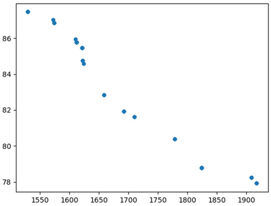
Figure 16.
Pareto solution.
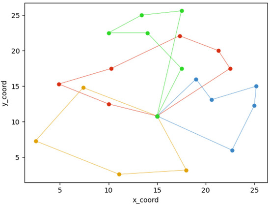
Figure 17.
Vehicle paths (different colors represent 5 vehicles for delivery route optimization).
When considering zero-carbon transportation, the delivery cost was CNY 1616.67, the zero-carbon transportation cost was CNY 87.47, a total of four vehicles were used for delivery, and the total amount of zero-carbon transportation was reduced to 174.94 kg.
4.5. Comparative Analysis
Table 5 shows the optimization results of single-objective optimization without zero-carbon transportation and multi-objective optimization without zero-carbon transportation.
Table 5.
Comparison of optimization results.
Compared with the single-objective optimization results that only considered the distribution cost, the multi-objective optimization results that considered both cost and zero-carbon transportation were considered. Only four vehicles could be used to complete the delivery, and the number of vehicles was reduced by one, which was more conducive to energy conservation and emission reduction. The distribution cost increased by CNY 28.93, while the zero-carbon traffic volume decreased by 81.48 kg, a decrease of 31.78%, and the total cost decreased by CNY 11.81. The distribution cost of single-objective optimization, which only considered the cost of distribution, was lower than the distribution cost of multi-objective optimization, which took into account both cost and zero-carbon transportation. If environmental costs are included in the cost accounting, it is obvious that the multi-objective optimization model proposed in this research has better solution results, which is more conducive to the sustainable development of China’s green logistics.
5. Sensitivity Analysis
5.1. Analysis of Impact of Traffic Congestion on Seafood Distribution in Ports
With the development of urban modernization, the increasing number of vehicles leads to congestion on urban roads. On the basis of the above examples, three different traffic congestion situations were set up, and the influence of traffic congestion on the path of urban logistics vehicles was explored through simulation experiments.
- Scenario 1: the road was completely clear, assuming a constant traffic congestion index of 1.
- Scenario 2: the road is congested; the road congestion index for different time periods is shown in Table 5.
- Scenario 3: the road is severely congested; and the road congestion index for different time periods is shown in Table 6.
Table 6. Traffic congestion index in each time period of Scenario 2.
Table 7 shows a comparison of the results of the three different traffic congestion situations, where denotes the number of vehicles used; TC represents total cost; RC stands for refrigeration cost; FC stands for fuel cost; CC stands for zero-carbon transportation cost; and CE stands for zero-carbon traffic.
Table 7.
Situation 3: traffic congestion index for each time period.
According to Table 8 and the comparative analysis of the simulation results, the following conclusions can be drawn:
Table 8.
Comparison of results under three traffic congestion conditions.
- (i)
- When the road was completely unblocked, the total cost was minimal, and the zero-carbon traffic volume was minimal.
- (ii)
- With the increase in urban road congestion index, the total cost of port seafood logistics distribution and zero-carbon transportation gradually increased; the results show that the total cost of zero-carbon transportation and distribution was positively correlated with congestion.
- (iii)
- With the increase in the urban road congestion index, the number of delivery vehicles increased to meet customer needs, reduce total costs, and meet delivery deadlines.
- (iv)
- With the same number of delivery vehicles, the higher the urban road traffic congestion index was, the greater the zero-carbon traffic volume was.
- (v)
- Although the congestion index changed significantly, the number of vehicles, total cost, refrigeration cost, fuel cost, and zero-carbon transportation cost did not change much. This shows that the port seafood distribution vehicles could carry out reasonable path planning under traffic congestion. The effectiveness of the multi-objective optimization model and the improved NSGA-II algorithm proposed in this research was demonstrated.
5.2. Analysis of Impact of Carbon Trading Prices on Port Seafood Distribution
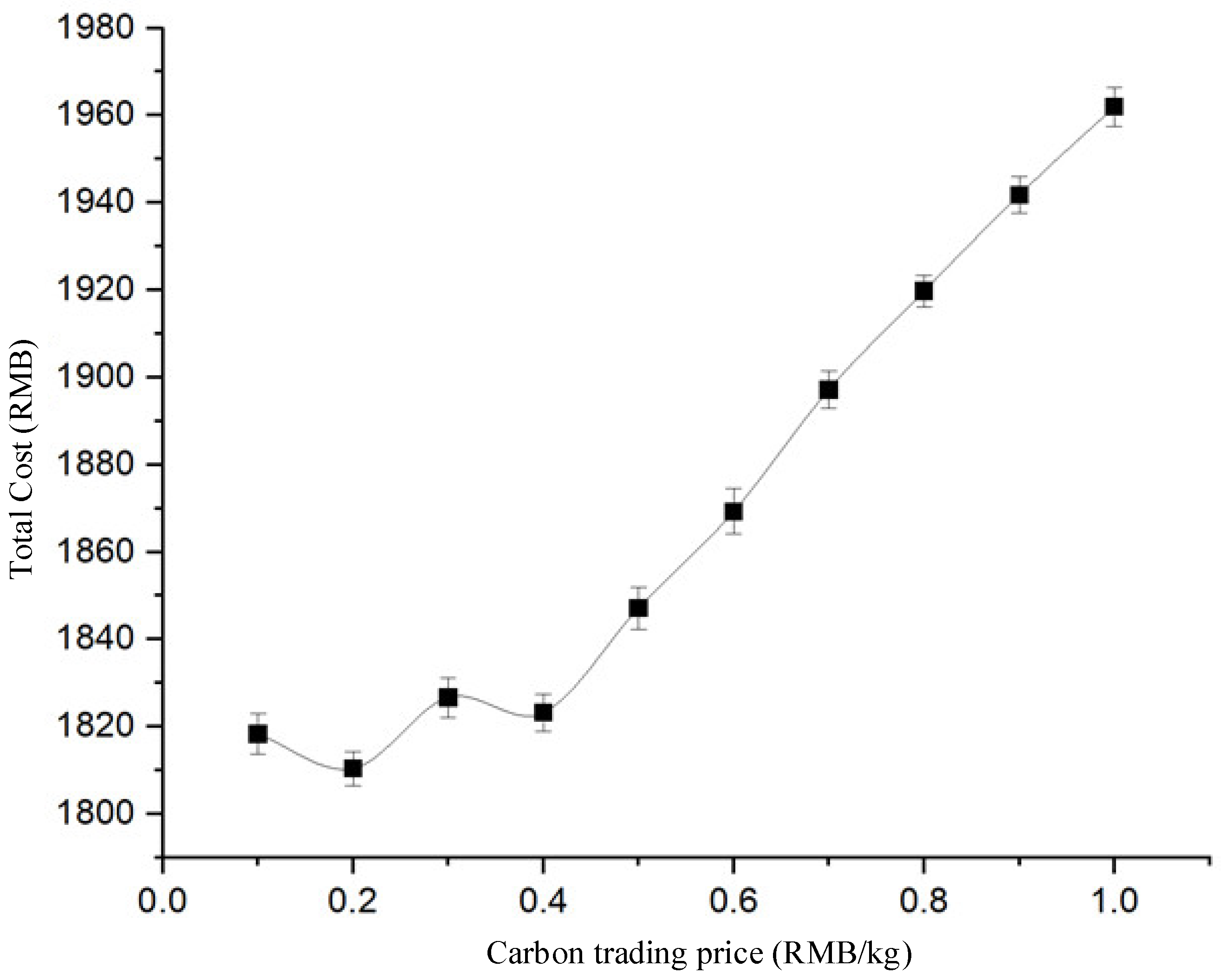
Based on Scenario 2, the impact of carbon trading price on the distribution results of port seafood was analyzed by changing the of carbon trading price. Under different carbon trading prices, , 10 simulation experiments were run independently, and the mean and variance of the total cost in the operation results were calculated. The total cost value was expressed as the mean of the total cost, and the error bar curve between the carbon trading price and the total cost was obtained, as shown in Figure 18. As can be seen from Figure 18, when the carbon trading price was , the total cost of port seafood logistics distribution was generally on the rise with the increase in the carbon trading price. However, when the minimum carbon trading price was 0.1 CNY/kg, the total cost was not the minimum value; this is because when the carbon trading price is low, the awareness of energy conservation and emission reduction in enterprises is weak. In order to complete the distribution task, the cost of zero-carbon transportation was ignored, which in turn increased the total cost. In addition, the variance of the total cost was within 5.2 under different carbon trading prices, which indicates that the improved NSGA-II algorithm designed in this research had good stability.
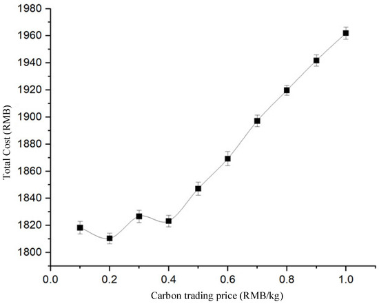
Figure 18.
The relationship between the carbon trading price and the total cost.
6. Conclusions
In this research, we fully considered traffic congestion and zero-carbon traffic in the process of seafood logistics distribution in urban ports, constructed a multi-objective optimization model, and conducted simulation analysis. The conclusions of this research are as follows:
- (i)
- We calculated the driving time of the vehicle and built a multi-objective optimization model. The road was divided and the traffic congestion index was used to find the time when the vehicle arrived at each customer point and the travel time. We analyzed the costs in the distribution process and established a multi-objective optimization mathematical model with the goal of minimizing the distribution cost of port seafood logistics and the minimum cost of zero-carbon transportation.
- (ii)
- Sensitivity analysis: The traffic congestion index, carbon trading price, and temperature difference between the inside and outside of the refrigerated truck were adjusted, respectively, and the distribution time and distribution cost were positively correlated with the congestion state of the road. With the increase in carbon trading prices, the total cost of port seafood logistics and distribution was generally on the rise.
In future research, the vehicle path optimization problem of port seafood logistics can also be further studied. This paper studies a distribution center and a single vehicle type, and research can further consider the path of simultaneous pick-up and delivery under multiple distribution centers and multiple types of vehicles.
Author Contributions
Conceptualization, R.X. and M.X.; methodology, H.X. and Z.Z.; software, R.X. and M.X.; validation, H.X. and Z.Z.; formal analysis, R.X. and M.X.; investigation, H. X. and Z.Z.; resources, R.X. and M.X.; data curation, H.X. and Z.Z.; writing—original draft preparation, R.X. and M.X.; writing—review and editing, H. X. and Z.Z.; visualization, R.X. and M.X.; supervision, H.X.; project administration, M.X.; funding acquisition, M.X. All authors have read and agreed to the published version of the manuscript.
Funding
This work was supported by the 2022 Sanya Science and Technology Innovation Project, China (No. 2022KJCX03), the Sanya Science and Education Innovation Park, Wuhan University of Technology, China (Grant No. 2022KF0028), and the Hainan Provincial Joint Project of Sanya Yazhou Bay Science and Technology City, China (Grant No. 2021JJLH0036).
Institutional Review Board Statement
Not applicable.
Informed Consent Statement
Not applicable.
Data Availability Statement
Data are available on request from the authors.
Acknowledgments
This paper was produced while the author was a visiting PhD student at the Centre of Excellence in Modelling and Simulation for Next Generation Ports (C4NGP), Department of Industrial Systems Engineering and Management, National University of Singapore (NUS), from 2024 to 2025.
Conflicts of Interest
The authors declare no conflicts of interest.
Nomenclature
| the vehicle set ; | |
| a collection of customer nodes to provide services to customer points; | |
| the cost per vehicle used; | |
| the speed at which the vehicle travels when the road is fully clear; | |
| the moment when the vehicle arrives at customer point ; | |
| the moment when the vehicle leaves customer point ; | |
| the distance from customer point to ; | |
| the congestion index for each sub-section; | |
| the heat load from refrigeration facilities while the vehicle is moving; | |
| the heat load from refrigeration facilities during vehicle unloading; | |
| the constant of the vehicle depreciation rate; | |
| the heat transfer rate; | |
| the heat transfer area of a refrigeration facility, with the unit ; | |
| the temperature difference between inside and outside of the refrigeration facility, with the unit ; | |
| the number of times the cooler has been opened; | |
| the vehicle ’s compartment volume; | |
| unit refrigeration cost; | |
| the unit price of diesel; | |
| the average unit value of seafood products in the port; | |
| carbon trading prices; | |
| the fuel consumption rate; | |
| vehicle loads; | |
| the weight of the vehicle when unloaded; | |
| zero-carbon transport allowances for businesses; | |
| the carrying capacity of the vehicle when it leaves customer point ; | |
| the coefficient of fresh spoilage in seafood in the port during vehicle transportation; | |
| the spoilage coefficient of fresh seafood in the port during the unloading of vehicles; | |
| the port seafood starting weight; | |
| the function of the degree of spoilage of port seafood; | |
| carbon credits purchased by companies; | |
| carbon credits sold by companies; | |
| the emission coefficient during vehicle driving; | |
| the vehicle refrigeration unit, mass cargo unit, distance, or emission factor; | |
| the penalty cost per unit of time of the early arrival of the vehicle; | |
| the penalty cost per unit of time for the late arrival of the vehicle; | |
| ; | |
| ; | |
| . |
References
- Moe, A.; Brigham, L.W.; Mitrova, T.; Stokke, O.S.; Yang, J.; Otsuka, N.; Kim, M.; Kim, S.J. Arctic economic development in uncertain times. In North Pacific Perspectives on the Arctic; Edward Elgar Publishing: Cheltenham, UK, 2024; pp. 24–49. [Google Scholar]
- Wang, J.; Zhang, Y. The effectiveness of legal framework of Arctic vessel-source black carbon governance. Environ. Sci. Pollut. Res. 2024, 31, 40472–40494. [Google Scholar] [CrossRef] [PubMed]
- Sanusi, S.M.; Paul, S.I.; Makarfi, A.M. Internet of Green Things (IoGT) for Carbon-Free Economy. In Data Science for Agricultural Innovation and Productivity; Bentham Science Publishers: Sharjah, United Arab Emirates, 2024; pp. 80–109. [Google Scholar]
- Zhang, Q.; Wan, Z.; Hemmings, B.; Abbasov, F. Reducing black carbon emissions from Arctic shipping: Solutions and policy implications. J. Clean. Prod. 2019, 241, 118261. [Google Scholar] [CrossRef]
- Wang, X.; Zhan, L.; Zhang, Y.; Fei, T.; Tseng, M.-L. Environmental cold chain distribution center location model in the semiconductor supply chain: A hybrid arithmetic whale optimization algorithm. Comput. Ind. Eng. 2024, 187, 109773. [Google Scholar] [CrossRef]
- Wang, Q.; Zhang, H.; Zhu, P.; Huang, J. Balancing energy security and marine pollution prevention: Legal challenges of utilizing nuclear power for decarbonizing maritime transportation in the Arctic region. Environ. Sci. Pollut. Res. 2024, 31, 40445–40461. [Google Scholar] [CrossRef] [PubMed]
- Carter, C.; Drouaud, F. Territory, ecological transition and the changing governance of ports. Territ. Politics Gov. 2024, 12, 374–394. [Google Scholar] [CrossRef]
- Oladosu, T.L.; Pasupuleti, J.; Kiong, T.S.; Koh, S.P.J.; Yusaf, T. Energy management strategies, control systems, and artificial intelligence-based algorithms development for hydrogen fuel cell-powered vehicles: A review. Int. J. Hydrog. Energy 2024, 61, 1380–1404. [Google Scholar] [CrossRef]
- Anwar, A.H.M.; Nora, N.N. A Review Approach to Understanding the Current Status of Port Resilience: Lessons Learned for GCC Ports. Climate-Resilient Cities; Springer: Cham, Switzerland, 2025; pp. 315–340. [Google Scholar]
- Kurniawan, T.A.; Meidiana, C.; Goh, H.H.; Zhang, D.; Othman, M.H.D.; Aziz, F.; Anouzla, A.; Sarangi, P.K.; Pasaribu, B.; Ali, I. Unlocking synergies between waste management and climate change mitigation to accelerate decarbonization through circular-economy digitalization in Indonesia. Sustain. Prod. Consum. 2024, 46, 522–542. [Google Scholar] [CrossRef]
- N’doye, I.; Zhang, D.; Alouini, M.S.; Laleg-Kirati, T.-M. Establishing and maintaining a reliable optical wireless communication in underwater environment. IEEE Access 2021, 9, 62519–62531. [Google Scholar] [CrossRef]
- Zhou, X.; Cao, J.; Xin, W. Predefined-time synchronization of coupled neural networks with switching parameters and disturbed by Brownian motion. Neural Netw. 2023, 160, 97–107. [Google Scholar] [CrossRef] [PubMed]
- Tong, Y.; Ren, Z.; Tong, D.; Fan, Z.; Feng, X. Combined finite-time state feedback for high-speed train systems with time-varying delays and disturbances. Int. J. Robust Nonlinear Control 2024, 34, 2184–2205. [Google Scholar] [CrossRef]
- Huang, J.-C.; Zeng, G.-Q.; Geng, G.-G.; Weng, J.; Lu, K.-D. SOPA-GA-CNN: Synchronous optimisation of parameters and architectures by genetic algorithms with convolutional neural network blocks for securing Industrial Internet-of-Things. IET Cyber-Syst. Robot. 2023, 5, e12085. [Google Scholar] [CrossRef]
- Xiao, X.; Li, H. Predicting mechanical responses of additively manufactured metamaterials with computational efficiency. CIRP J. Manuf. Sci. Technol. 2024, 52, 149–158. [Google Scholar] [CrossRef]
- Qi, Y.; Tang, Y.; Yu, K. Full Differential Privacy Preserving for Switched LPV Systems. IEEE Trans. Syst. Man Cybern. Syst. 2024, 54, 3153–3163. [Google Scholar] [CrossRef]
- Dornaika, F.; Bi, J.; Zhang, C. A unified deep semi-supervised graph learning scheme based on nodes re-weighting and manifold regularization. Neural Netw. 2023, 158, 188–196. [Google Scholar] [CrossRef] [PubMed]
- Shi, Y.; Yang, J.; Han, Q.; Song, H.; Guo, H. Optimal decision-making of post-disaster emergency material scheduling based on helicopter–truck–drone collaboration. Omega 2024, 127, 103104. [Google Scholar] [CrossRef]
- Xiao, J.; Anwer, N.; Li, W.; Eynard, B.; Zheng, C. Dynamic Bayesian network-based disassembly sequencing optimization for electric vehicle battery. CIRP J. Manuf. Sci. Technol. 2022, 38, 824–835. [Google Scholar] [CrossRef]
- Kaššaj, M.; Peráček, T. Synergies and Potential of Industry 4.0 and Automated Vehicles in Smart City Infrastructure. Appl. Sci. 2024, 14, 3575. [Google Scholar] [CrossRef]
- Nekit, K.; Kolodin, D.; Fedorov, V. Personal data protection and liability for damage in the field of the internet of things. Jurid. Trib. J. 2020, 10, 80–93. [Google Scholar]
- Gonçalves, M.; Salgado, C.; de Sousa, A.; Teixeira, L. Data Storytelling and Decision-Making in Seaport Operations: A New Approach Based on Business Intelligence. Sustainability 2025, 17, 337. [Google Scholar] [CrossRef]
- GB/T18354-2021; Logistics Terminology. Chinese Standard: Beijing, China, 2021.


Disclaimer/Publisher’s Note: The statements, opinions and data contained in all publications are solely those of the individual author(s) and contributor(s) and not of MDPI and/or the editor(s). MDPI and/or the editor(s) disclaim responsibility for any injury to people or property resulting from any ideas, methods, instructions or products referred to in the content. |
© 2025 by the authors. Licensee MDPI, Basel, Switzerland. This article is an open access article distributed under the terms and conditions of the Creative Commons Attribution (CC BY) license (https://creativecommons.org/licenses/by/4.0/).