A Novel Adaptive Fault-Tolerant Cooperative Control for Multi-PMLSMs of Low-Carbon Urban Rail Linear Traction Systems

Abstract

Permanent magnetic linear synchronous motors (PMLSMs) have emerged as a promising solution for low-carbon urban rail transit systems due to their superior energy efficiency. However, their widespread adoption is hindered by significant challenges in achieving high-precision cooperative control and fault-tolerant operation across multi-PMLSMs. To address these issues, this paper proposed a novel composite observer-based adaptive fault-tolerant cooperative control framework, which enables reliable speed synchronization in multi-PMLSM urban rail traction systems through three key innovations. Initially, the stuck fault of the actuator is modeled based on the PMLSM dynamic model, and a composite observer is proposed to estimate lumped disturbances and actuator faults simultaneously, enhancing the system’s robustness against uncertainties and faults. A novel sliding mode control scheme with adaptive parameters is subsequently developed to compensate for disturbances and improve tracking accuracy. Furthermore, two event-triggered schemes are devised to reduce the communication burden, ensuring efficient data transmission without compromising control performance. The proposed method ensures high-precision synchronization and fault tolerance under actuator stuck faults, bias faults, and external disturbances, as validated by simulation results. By improving energy efficiency and reducing communication load, the proposed method contributes to the development of low-carbon urban rail transit systems, aligning with global sustainability goals.

1. Introduction

The urban rail transit system is an important transportation artery for large and medium-sized cities [1]. In recent years, with the advancement of urbanization in the world, urban rail transit has developed rapidly [2], with a significant increase in the number of operating lines, and the total percentage of its energy consumption has been constantly increasing [3]. Therefore, in the context of carbon neutrality, the development of novel low-carbon and energy-saving urban rail transit technologies is urgently needed [4]. In this vein, the traction system is the most power-consuming part, and its average energy consumption accounts for more than 50% of the total energy consumption of urban rail transit systems [5]. At present, rotation asynchronous motors are the most widely used type of drive motor for urban rail transit traction systems [6], which exhibit limitations in operational efficiency, high mechanical energy loss, and poor adaptation of load characteristics to train demand, and thus have high energy consumption. As a new type of traction motor, permanent magnetic linear synchronous motors (PMLSMs) can directly convert electrical energy into mechanical energy for linear motion without the help of any intermediate conversion mechanisms [7]. Meanwhile, with the help of permanent magnets, PMLSMs do not require additional power consumption to maintain their magnetic field during motor operation [8]. Therefore, PMLSMs have significant advantages in terms of operating efficiency and energy savings [9], which can reduce the average energy consumption by 20%–30% compared with rotation asynchronous motors; thus, this is an ideal type of traction motor for realizing low-carbon urban rail transit systems [10].

Although urban rail transit trains with PMLSMs as the source of traction power have high operational efficiency and excellent energy-saving performance [11], the characteristics of strong coupling, uncertainty, nonlinearity, and fault-proneness greatly increase the difficulty of the high-precision control of PMLSMs [12]. Moreover, each urban rail transit train contains multiple PMLSMs, and each PMLSM is expected to run at the same pace [13]. As significant desynchronization events occur, the train may shake or side-tip, which directly threatens the safety of the train [14]. As a result, it is crucial to design a high-performance adaptive fault-tolerant cooperative controller to guarantee the synchronization performance of the multi-PMLSMs of urban rail transit trains [15]. At present, PMLSM control strategies have been widely studied, such as fuzzy backstepping control in [16], loss minimization control in [17], and iterative learning PID control in [18]. Yet, they fail to maintain the linear motors in synchronization and may introduce coupling errors especially in multi-motor cooperative operation. Aimed at keeping multi-PMLSMs operating synchronously, numerous researchers have proposed a variety of better control methods. In [19], a variable-gain adjacent cross-coupled controller is proposed for the multi-PMLSMs system, realizing the coordinated motion of the system. In [20], a model predictive control method is presented for a networked linear induction motor system, which makes the tracking performance accurate and synchronous. In [21], an adaptive control strategy with online parameter identification is designed for integrated PMLSMs, enhancing positioning and the coordination accuracy of the system. In [22], a sliding mode variable structure deviation coupling approach is proposed to improve the performance of multi-PMLSM systems, including synchronization performance. From the aforementioned references, it can be found that many researchers have realized cooperative control for multiple PMLSMs, which can be applied to multi-PMLSMs of urban rail transit. However, MPC suffers from computational complexity and sensitivity to model inaccuracies, limiting real-time applications; the parameter design of robust control is too conservative and complex, and again the control performance depends on the accuracy of model building. Moreover, due to the complexity of the system, actuator faults may inevitably occur [23]; thus, the wrong signals received may induce safety hazards. The critical challenge lies in developing robust fault-tolerant control mechanisms that can maintain system stability and prevent catastrophic failures during actuator faults, which remains an open research problem [24].

Faults may cause adverse effects to multi-PMLSMs, such as longer synchronization times and low tracking accuracy. In recent years, for the sake of decreasing the influence brought by faults on industrial systems, some authors have proposed fault-tolerant control, a method to guarantee that the system runs safely when actuator faults arise. For example, in [25], an adaptive fault-tolerant control strategy is devised for dual three-phase permanent magnetic synchronous machine drives, which increases the reliability of the drive system by applying unified fault-tolerant reference currents. In [26], a fault estimation and tolerant control is designed for high-speed trains, using real-time fault estimation and control of the system state to track the desired trajectory accurately. In [27], an active fault-tolerant cooperative control scheme is established to maintain the desired tracking performances and cooperative performances, achieving the cooperative control of multiple high-speed trains affected by unknown parameters and actuator faults. Also, in [28], a model-free adaptive iterative learning control method based on data-driven control is proposed, which achieves the cooperative control of multiple subway trains in the presence of speed sensor faults and provides overspeed protection, ensuring that the trains operate within a safe speed range, etc. To sum up, fault-tolerant control is an effective method to handle various faults and to make the system more resistant to the threat of faults [29]. If applied in multi-PMLSMs, fault-tolerant control will have the potential to ameliorate reliability under the actuator faults of the system.

Moreover, communication between multi-PMLSMs requires a large amount of data, which causes a waste of communication and computation resources, resulting in negative influences such as delays in train signal response [30]. A lot of research has been conducted on this problem, and some researchers have proposed an event-trigger scheme to avoid frequent communication [31]. Different from traditional serial communication, the event-triggered scheme, which the signals will be sent only if the trigger condition is satisfied, has the potential to handle this problem. In [32], an event-triggered adaptive asymptotic tracking control scheme is proposed and applied to linear motors, where communication burden and computational complexity are reduced. In [33], an event-triggered adaptive saturated fault-tolerant control is proposed for a linear motor system, which contributes to the reduction in communication resources. Consequently, an event-triggered scheme is an effective approach for alleviating communication burden and can further improve the performance of the multi-PMLSMs. Devising an event-triggered scheme is a feasible attempt to improve the communication efficiency of the multi-PMLSMs of urban rail transit.

Inspired by the factors above, to reduce the influence brought by actuator stuck faults and realize high-performance cooperative control, this paper has proposed a novel adaptive fault-tolerant cooperative control for multi-PMLSMs to realize high-performance low-carbon urban rail linear traction systems. The main contributions can be concluded as follows:

• A cooperative approach based on sliding mode control (SMC) is proposed for multi-PMLSMs in this study. At the core of the devised control scheme, the estimated values shape the sliding manifold. Furthermore, the controller incorporates an adaptive parameter and a sophisticated adaptive mechanism, both of which significantly contribute to enhancing the convergence properties and overall robustness of the proposed method.
• An adaptive fault-tolerant controller based on a composite observer is designed for multi-PMLSMs, which aims to stabilize the system under the condition of actuator stuck faults.
• An event-trigger mechanism is constructed for multi-PMLSMs. In this article, the tracking error and estimation error are utilized to design a time-varying trigger threshold, enhancing the controller’s robustness.

The subsequent sections of this article are structured in the following manner. Section 2 defines and outlines the problems aimed to be addressed. Section 3 details the construction and deduction of the proposed strategy. In Section 4, the simulation results are presented to validate and demonstrate the efficacy of our approach. Section 5 brings this article to a conclusion by summarizing the key findings.

2. Preliminaries and Problem Formulation

2.1. System Description

The structure of the urban rail linear traction system depicted in Figure 1 harnesses the magnetic field generated by permanently installed magnets (with alternating N and S poles) along the track. This mobile magnetic field interacts with the linear motor located at the bottom of every train, which consists of a stator and a mover. The electromagnetic coils on the stator, labeled A, Z, Y, B, C, and X, produce thrust in response to the moving magnetic field. The interaction between the traveling magnetic field and the excitation magnetic field propels the train forward in accordance with the principles of electromagnetic induction. Each train (such as the nth train, the second train, and the leader train) is equipped with communication devices that maintain synchronization with the preceding and following trains through communication signals, ensuring a safe distance is kept. The leading train may also receive instructions from the control center to coordinate the operation of the entire train formation. This system is designed to leverage the magnetic properties of permanent magnets to achieve efficient, low-friction traction, thereby enhancing the operational efficiency and passenger comfort of the train.

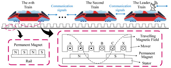
Figure 1. Structure of urban rail linear traction system.

2.2. Dynamic Model of Multi-PMLSMs

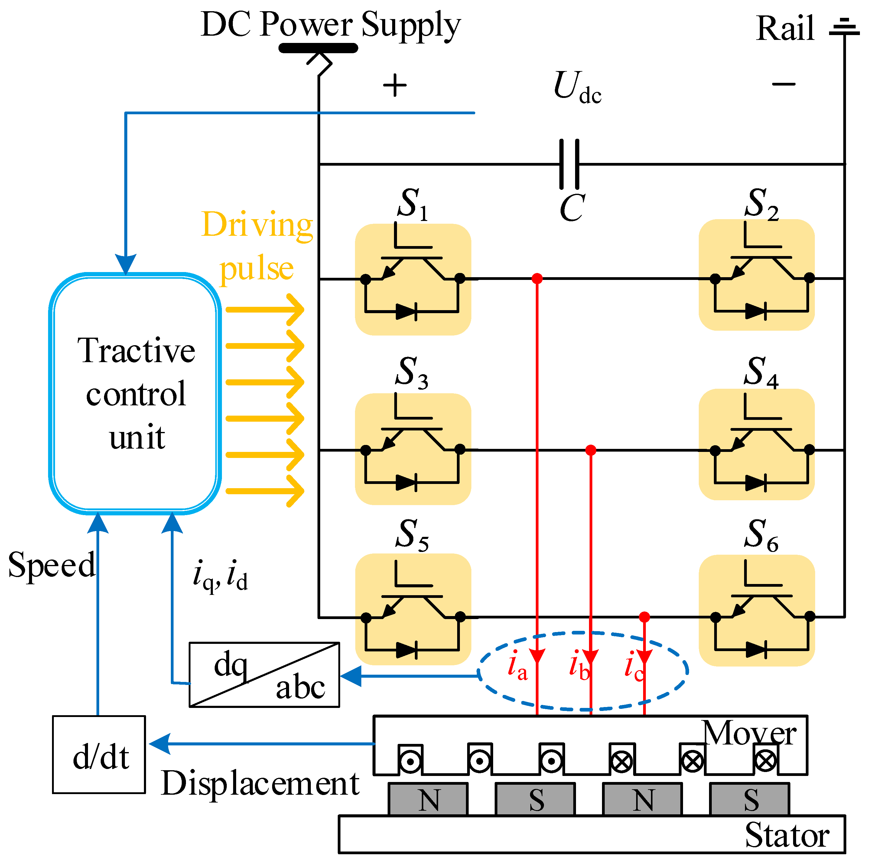
Figure 2 illustrates a driving circuit for a PMLSM. The system is powered by a direct current (DC) source, with a capacitor C smoothing the voltage to provide a stable DC voltage Udc for the motor. A traction control unit modulates the motor’s operation based on the train’s speed and displacement. This control unit generates driving pulses that control the on–off states of six power switches (S1 to S6), which form a three-phase H-bridge circuit and regulate the three-phase currents (ia, ib, and ic) of the motor. The stator of the motor is equipped with three-phase windings, while the mover (rotor) is mounted with permanent magnets, creating a permanent magnetic field. As the three-phase currents pass through the stator windings, they generate a rotating magnetic field that interacts with the permanent magnets on the mover, producing the thrust required for linear motion. The figure also displays feedback loops for current and displacement, which are used for closed-loop control to precisely regulate the motor’s speed and position. Through this control method, the PMLSM is capable of achieving efficient and accurate linear motion.

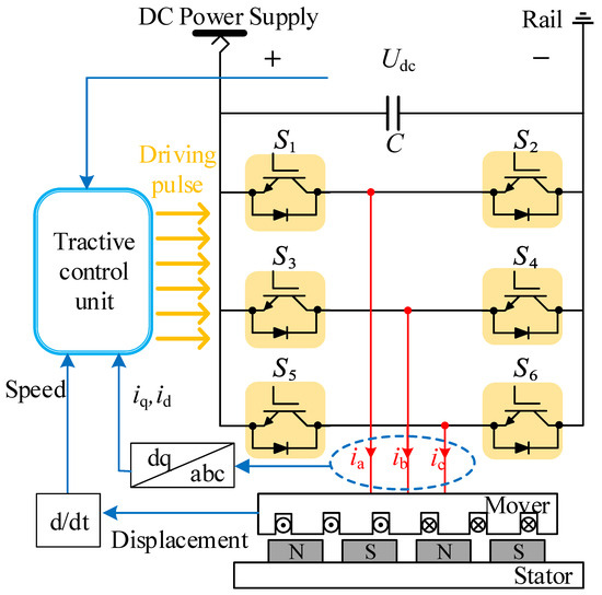
Figure 2. Electric circuit of a single PMLSM.

The dynamic model of the PMLSM in d-q axis is expressed as follows [34]

$$\left\{\begin{array}{c}{L}_d{\displaystyle \frac{d{i}_d}{dt}}=-R_s{i}_d+\omega L_q{i}_q+u_d\hfill \\ L_q{\displaystyle \frac{d{i}_q}{dt}}=-R_s{i}_q-\omega L_d{i}_d+u_q-\omega {\varphi }_{pm}\hfill \\ Ma=K_f{i}_q-Bv-F_d\hfill \end{array}\right.$$

(1)

where $L_d$, $L_q$ are the d-q axis inductance; $i_d$, $i_q$, $u_d$, and $u_q$ are the d-q axis current and voltage; v represents the speed of the motor; $\omega$ is the electrical angular velocity of the mover, which has a linear relationship with v; $R_s$ denotes the armature resistance; ${\varphi }_{pm}$ means the permanent magnet flux; M is the mass of motor; a is the acceleration; B is the viscous friction coefficient; and $F_d$ denotes the resistance force.

The vector is defined as $x={\left[x_1,x_2,x_3,x_4,x_5,x_6\right]}^T={\left[x_{dis},v,q_d,i_d,q_q,i_q\right]}^T$ and the speed of motor v is defined as the output; the system can be written in the following form:

$$\left\{\begin{array}{c}{\dot{x}}_{2i-1}(t)=x_{2i}(t)\hfill \\ {\dot{x}}_{2i}(t)=f_{di}(x)+g_i{u}_i(t)\hfill \\ y(t)=x_2(t)\hfill \end{array}\right.$$

(2)

where $x_{dis}$ is the displacement of the motor; $q_d$ and $q_q$ are the quantity of electric charge that are just used to represent the integral results of d-q axis current with respect to time; $i=1,2,3$; $g_i$ means the control gains; and $u_i$ denotes the input.

Considering the following actuator fault model,

$$\begin{array}{c}\hfill u_{af,i}(t)=z_i{l}_i{u}_{di}(t)+(1-z_i)u_{di}(t_{oc})+c_{ai}{u}_{bi}(t)\end{array}$$

(3)

where $z_i=0$ when actuator fault occurs and the occurrence time is denoted as $t_{oc}$; $l_i$ is the loss of effectiveness, constrained by upper bound $l_{ub}$ and lower bound $l_{lb}$, whose changing rate is no more than $\pm l_r$, a constant; $u_{di}$ represents the designed control input; $c_{ai}$ is a constant parameter; and $u_{bi}$ means bias fault.

Substituting (3) into (2) and considering system uncertainties and disturbance, the system becomes

$$\left\{\begin{array}{c}{\dot{x}}_{2i-1}(t)=x_{2i}(t)\hfill \\ {\dot{x}}_{2i}(t)=f_{di}(x)+g_i(z_i{l}_i{u}_{di}(t)+(1-z_i)u_{di}(t_{oc})\hfill \\ +c_{ai}{u}_{bi}(t))+u_{si}(x,t)+d_i(t)\hfill \\ y(t)=x_2(t)\hfill \end{array}\right.$$

(4)

where $u_{si}(x,t)$ is the system uncertainty and $d_i$ represents disturbance.

Assumption 1.

The dynamic function can be represented as

$$\begin{array}{c}\hfill f_{di}(x)=f_{di}(y)+f_{un,i}(x)\end{array}$$

(5)

where $f_{un,i}(x)$ is unknown.

Assumption A2.

The nonlinear system unknown function $u_{si}(x,t)$ can be depicted as the product of an unknown constant $k_{gi}$ and a known function $g(\hat{x},t)$.

$$\begin{array}{c}\hfill u_{si}(x,t)=k_{gi}g(\hat{x},t)\end{array}$$

(6)

The primary objective of this article is to address the challenge of tracking a nonlinear system while efficiently alleviating communication resource consumption. Specifically, the objective is to devise a robust fault-tolerant control scheme that can mitigate the effects of instability. Furthermore, an event-triggered controller will be introduced to minimize the load on transmission channels.

2.3. Directed Graph Theory

Define a directed topological graph $G=(V,E,\mathit{A})$ as a multiple motors system topological graph. $V=\{v_1,\cdots ,v_n\}$ is the set of nodes; $E\subseteq V\times V$ is the set of edges. If there is any information transmitted from node j to node k, j has an edge with k, which is denoted as $(v_j,v_k)\in E$. $\mathit{A}={\left[a_{jk}\right]}_{n\times n}$ is an adjacency matrix. If the positions of $v_j$ and $v_k$ are exchanged and they still belong to the set of edges, $a_{jk}=1$; otherwise, $a_{jk}=0$. As for the condition $j=k$, specifically define $a_{jj}=0$. Define $\mathit{D}=\mathrm{diag}(d_1,\cdots ,d_n)$, where $d_j={\displaystyle \sum _{k=1}^n}{a}_{jk}$; $\mathit{B}=\mathrm{diag}(b_1,\cdots ,b_n)$; and $b_j=1$ if the node j communicates with the leader; otherwise, $b_j=0$ [35].

3. Proposed Method

In this section, an adaptive event-triggered SMC approach is devised for multi-PMLSM systems. Specifically, a novel observer is first proposed to acquire the combined disturbance and state information. With the estimated data, an adaptive SMC scheme integrated with an event-trigger mechanism is then designed, which allows for the maintenance of the trajectory tracking capability.

3.1. Event-Trigger Condition Design

In this part, two event-triggered generators are designed to release the communication burden, one ahead of the actuator while the other is after the controller [33]. Assume that the current output is $y_i(t)$ and the output signal when the w-th event-trigger happens is $y_i(t_w)$, where $w=0,1,2,...$ and $t_0=0$. The event-trigger condition is defined as

$$\begin{array}{c}\hfill e_y^{T}W{e}_y\le k_{r}y{(t_w)}^{T}Wy(t_w)\end{array}$$

(7)

where W is a weighting matrix; $k_r$ is a parameter satisfying $0<k_r<1$; $e_y=y(t_w)-y(t)$.

Likewise, the output of the controller is recorded as $u_{di}(t)$, while the one when event-triggered is $u_{di}(t_s)$, where $t_s$ is the triggering time and $s=0,1,2,...$.

3.2. Composite Observer Design

For the sake of estimating the state variables of the system, an observer is proposed in this paper that further assists to enhance the control performance. The composite observer is designed to integrate multiple types of estimation functions and is capable of handling multiple uncertainties and fault types in the system simultaneously, including the estimation of the lumped disturbance and actuator fault estimation. The observer is designed as

$$\left\{\begin{array}{c}{\dot{\hat{x}}}_{2i-1}(t)={\hat{x}}_{2i}(t)+K_{og}(y_i(t_n)-{\hat{y}}_i)\hfill \\ {\dot{\hat{x}}}_{2i}(t)={\hat{f}}_{di}(x)+z_i{\hat{l}}_i{g}_i{u}_{di}(t)+u_{si}(x,t)+c_{ei}(t)\hfill \\ \hat{y}(t)={\hat{x}}_2(t)\hfill \end{array}\right.$$

(8)

where the variables with a hat are the estimates of the corresponding variables; $K_{og}$ is the observer gain. $c_{ei}(t)$ is the estimation error compensator.

Define $\mathsf{\ell }=-z_i{u}_{di}{(t)}^T{g}_i^T{C_{OI}}^{T}P{e}_v$; ${\dot{\hat{l}}}_i(t)=0$ if ${\hat{l}}_i$ reaches the upper bound $l_{ub}$ while $\mathsf{\ell }>0$ or ${\hat{l}}_i$ reaches the lower bound $l_{lb}$ while $\mathsf{\ell }<0$; otherwise, ${\dot{\hat{l}}}_i(t)=\mathsf{\ell }$; $C_{OI}={\left[O,I\right]}^T$; $e_{vi}={\left[\begin{array}{cc}{e}_{2i-1}& e_{2i}\end{array}\right]}^T$, $e_{2i}=x_{2i}-{\hat{x}}_{2i}$; $e_{2i-1}=x_{2i-1}-{\hat{x}}_{2i-1}$. $c_{ei}(t)$ is defined as

$$\begin{array}{cc}\hfill c_{ei}(t)=& {\displaystyle \frac{C_{OI}P{e}_{vi}}{{∥e_{vi}^{T}P{C}_{OI}∥}^2}}(∥e_{vi}^{T}P{C}_{IO}{K}_{og}{e}_y∥+∥e_{vi}^{T}P{D}_M{e}_{vi}∥\hfill \\ \hfill & -2{\hat{k}}_s∥e_{vi}^{T}P∥∥v_{di}∥-2l_y)\hfill \end{array}$$

(9)

where $l_y=2(l_{ub}-l_{lb})(l_r+l_{ub}-l_{lb})$. $D_M$ is a designed matrix. ${\hat{k}}_{si}$ is the estimation of $k_{si}$, which is an unknown mentioned later, as well as the vectors to be designed—$v_{di}$. $C_{IO}={\left[\begin{array}{cc}I& O\end{array}\right]}^T$.

Based on Assumptions 1 and 2, system uncertainty and dynamic equation can be represented as ${\hat{u}}_{si}(x,t)={\hat{k}}_{gi}g(\hat{x},t)$ and ${\hat{f}}_{di}(x)=f_{di}(y)+{\hat{f}}_{un,i}(x)$. As ${\dot{e}}_{2i-1}={\dot{x}}_{2i-1}-{\dot{\hat{x}}}_{2i-1}$, ${\dot{e}}_{2i}={\dot{x}}_{2i}-{\dot{\hat{x}}}_{2i}$, ${\dot{e}}_{2i-1}$, and ${\dot{e}}_{2i}$ can be obtained by calculating the difference.

$$\begin{array}{c}\hfill {\dot{e}}_{2i-1}=e_{2i}-K_{og}(y(t_n)-\hat{y}(t))\end{array}$$

(10)

$$\begin{array}{cc}\hfill {\dot{e}}_{2i}=& {\tilde{f}}_{di}(x)+z_i{g}_i{\tilde{l}}_i{u}_{di}(t)+{\tilde{u}}_{si}(x,t)-c_{ei}(t)\hfill \\ \hfill & +(1-z_i)g_i{u}_{di}(t_{oc})+c_{ai}{g}_i{u}_{bi}(t)+d_i(t)\hfill \end{array}$$

(11)

where ${\tilde{l}}_i=l_i-{\hat{l}}_i$, ${\tilde{u}}_{si}(x,t)=u_{si}(x,t)-{\hat{u}}_{si}(x,t)$, and ${\tilde{f}}_{di}(x)=f_{di}(x)-{\hat{f}}_{di}(x)$.

The error dynamics can be reformulated in matrix form as

$$\begin{array}{cc}\hfill {\dot{e}}_v=& A_K{e}_{vi}(t)+u_{sv}(x,t)+C_{OI}({\tilde{f}}_{di}+z_i{\tilde{l}}_i{g}_i{u}_{di}(t))\hfill \\ \hfill & -C_{IO}{K}_{og}{e}_y-C_{OI}{c}_{ei}(t)+d_{lump}(t)\hfill \end{array}$$

(12)

where $A_K=\left[\begin{array}{cc}-K_{og}I& I\\ O& O\end{array}\right]$, $u_{sv}=\left[\begin{array}{c}0\\ u_{si}(x,t)\end{array}\right]$, $d_{lump}(t)=\left[\begin{array}{c}0\\ (1-z_i)g_i{u}_{di}(t_{oc})+c_{ai}{g}_i{u}_{bi}(t)+d_i(t)\end{array}\right]$.

Assuming that the lumped disturbance (load fluctuations, motor parameter perturbation, etc.) is restricted by $∥d_{lump}(t)∥\le k_{si}∥v_{di}(t)∥$, $v_{di}(t)$ is designed as

$$\begin{array}{c}\hfill v_{di}(t)={\int }_0^t{e}_{vi}(t)dt+e_{vi}(t)-h(t)\end{array}$$

(13)

where $h(t)$ can be updated as

$$\begin{array}{cc}\hfill \dot{h}(t)=& A_K{e}_{vi}(t)+C_{OI}{z}_i{\tilde{l}}_i{g}_i{u}_{di}(t)-C_{IO}{K}_{og}{e}_y\hfill \\ \hfill & -C_{OI}{c}_{ei}(t)-p(t)\hfill \end{array}$$

(14)

$$\begin{array}{c}\hfill p(t)=-(a_p+{\hat{k}}_{si})v_{di}+e_{vi}(t)\end{array}$$

(15)

where $a_p$ is a positive constant and ${\hat{k}}_{si}$ is designed as

$$\begin{array}{c}\hfill {\dot{\hat{k}}}_{si}=a_p({∥v_{di}∥}^2+∥e_{vi}^{T}P∥∥v_{di}∥)\end{array}$$

(16)

Deriving $v_{di}$ with respect to t, one can obtain

$$\begin{array}{cc}\hfill {\dot{v}}_{di}(t)=& e_{vi}(t)+{\dot{e}}_{vi}(t)-A_K{e}_{vi}(t)+C_{OI}{z}_i{\tilde{l}}_i{g}_i{u}_{di}(t)\hfill \\ \hfill & -C_{IO}{K}_{og}{e}_y-C_{OI}{c}_{ei}(t)-p(t)\hfill \end{array}$$

(17)

The estimation of lumped disturbance is assumed as

$$\begin{array}{c}\hfill {\hat{d}}_{lump}(t)=-[e_{vi}(t)+p(t)]\end{array}$$

(18)

Theorem 1.

The estimation errors $e_{2i-1}$, $e_{2i}$, $u_{si}$, and $f_{di}$ will ultimately converge at zero if

$$\begin{array}{c}\hfill P(A_K-D_M)+{(A_K-D_M)}^{T}P<0\end{array}$$

(19)

is satisfied, where P is a positive symmetric matrix.

Proof. 

Construct Lyapunov function $V_1(t)$ as

$$\begin{array}{cc}\hfill V_1(t)=& e_{vi}^{T}P{e}_{vi}+{v_{di}}^T{v}_{di}+{\displaystyle \frac{{\tilde{k}}_{si}^T{\tilde{k}}_{si}}{a_p}}+{{\tilde{k}}_g}^T{\tilde{k}}_g\hfill \\ & +{\tilde{f}}_{un,i}^T(x){\tilde{f}}_{un,i}(x)+{\tilde{l}}_i^T{\tilde{l}}_i\hfill \end{array}$$

(20)

where ${\tilde{k}}_{gi}={\hat{k}}_{gi}-k_{gi}$, ${\tilde{f}}_{un,i}(x)={\hat{f}}_{un,i}(x)-f_{un,i}(x)$, and $k_g={\left[\begin{array}{cc}0& k_{gi}\end{array}\right]}^T$; $k_g$ and ${\hat{f}}_{un,i}(x)$ are updated by ${\dot{\hat{k}}}_g=-g{(x,t)}^T[P{e}_{vi}+v_{di}(t)]$ and ${\dot{\hat{f}}}_{un,i}=-g{(x,t)}^T[P{e}_{vi}(t)+v_{di}(t)]$.

Take the derivative of $V_1$ and substitute the terms above into it; then,

$$\begin{array}{cc}\hfill {\dot{V}}_1=& 2e_{vi}^{T}P{\dot{e}}_{vi}+2{v_{di}}^T{\dot{v}}_{di}+{\displaystyle \frac{2{\tilde{k}}_{si}^T{\dot{\tilde{k}}}_{si}}{a_p}}\hfill \\ & +2[{\tilde{f}}_{un,i}^T(x){\dot{\tilde{f}}}_{un,i}(x)+{\tilde{l}}_i^T{\dot{\tilde{l}}}_i+{\tilde{k}}_g^T{\dot{\tilde{k}}}_g]\hfill \\ \hfill =& 2e_{vi}^{T}P[A_K{e}_v+u_{sv}(x,t)-C_{IO}{K}_{og}{e}_y\hfill \\ & +C_{OI}({\tilde{f}}_{di}(x)+z_i{\tilde{l}}_i{g}_i{u}_{di}(t)-c_{ei}(t))+d_{lump}(t)]\hfill \\ & +2v_{di}{(t)}^T[{\tilde{u}}_{si}(x,t)+C_{OI}{\tilde{f}}_{di}(t)+{\tilde{d}}_{lump}(t)]\hfill \\ & -2{\tilde{k}}_{si}^T({∥v_{di}∥}^2+∥e_{vi}^{T}P∥∥v_{di}∥)\hfill \\ & +2[{{\tilde{k}}_g}^T{\dot{\tilde{k}}}_g+{\tilde{f}}_{un,i}^T(x){\dot{\tilde{f}}}_{un,i}(x)+{\tilde{l}}_i^T{\dot{\tilde{l}}}_i]\hfill \end{array}$$

(21)

Combining the fact that $l_i(t)$ is bounded and ${\dot{l}}_i(t)$ is restricted by $l_r$, the estimation error is no bigger than the difference of upper bound and lower bound. Through mathematical derivation, we obtain

$$\begin{array}{cc}& e_{vi}^{T}P{C}_{OI}{z}_i{\tilde{l}}_i{g}_i{u}_{di}(t)+{\tilde{l}}_i^T{\dot{\tilde{l}}}_i\hfill \\ \hfill =& z_i{e}_{vi}^{T}P{C}_{OI}{g}_i{u}_{di}(t){\tilde{l}}_i+{\tilde{l}}_i^T({\dot{l}}_i-z_i{u}_{di}{(t)}^T{g}_i^T{C_{OI}}^{T}P{e}_{vi})\hfill \\ \hfill =& {\tilde{l}}_i^T({\dot{l}}_i+{\tilde{l}}_i)-{\tilde{l}}_i^T{\tilde{l}}_i\hfill \\ \hfill \le & (l_{ub}-l_{lb})(l_r+l_{ub}-l_{lb})\hfill \end{array}$$

(22)

Noticing that

$$\begin{array}{cc}& 2e_{vi}^{T}P[u_{sv}(x,t)+C_{OI}{\tilde{f}}_{di}(x)]+2[{\tilde{f}}_{un,i}^T(x){\dot{\tilde{f}}}_{un,i}(x)\hfill \\ & +{\tilde{k}}_g^T{\dot{\tilde{k}}}_g]+2v_{di}{(t)}^T[{\tilde{u}}_{si}(x,t)+C_{OI}{\tilde{f}}_{di}(x)]\hfill \\ \hfill =& 2[e_{vi}^{T}Pg(x,t)+v_{di}{(t)}^{T}g(x,t)]{\tilde{k}}_g\hfill \\ & +2[e_{vi}^{T}P{C}_{OI}+v_{di}{(t)}^T{C}_{OI}]{\tilde{f}}_{di}(x)\hfill \\ & -2{\tilde{k}}_g^{T}g{(x,t)}^T[P{e}_{vi}+v_{di}(t)]\hfill \\ & -2{\tilde{f}}_{un,i}^T(x)C_{OI}^T[P{e}_{vi}(t)+v_{di}(t)]\hfill \\ \hfill =& 0\hfill \end{array}$$

(23)

Also, by substituting in (18), it can be obtained that

$$\begin{array}{cc}& 2e_{vi}^{T}P{d}_{lump}+2v_{di}^T{\tilde{d}}_{lump}-2{\tilde{k}}_{si}^T[∥e_{vi}^{T}P∥∥v_{di}∥+{∥v_{di}∥}^2]\hfill \\ \hfill \le & 2k_{si}(∥e_{vi}^{T}P∥∥v_{di}∥+{∥v_{di}∥}^2)-2v_{di}^T(a_p+{\hat{k}}_{si})v_{di}\hfill \\ & -2{\tilde{k}}_{si}^T[∥e_{vi}^{T}P∥∥v_{di}∥+{∥v_{di}∥}^2]\hfill \\ \hfill =& -2a_p{∥v_{di}^T∥}^2+2{\hat{k}}_{si}∥e_{vi}^{T}P∥∥v_{di}∥\hfill \end{array}$$

(24)

Substituting (22), (23), and (24) into (21), it can get represented as

$$\begin{array}{cc}\hfill {\dot{V}}_1=& 2e_{vi}^{T}P[(A_K-D_M)e_{vi}-C_{IO}{K}_{og}{e}_y-C_{OI}{c}_{ei}]\hfill \\ & +2[e_{vi}^{T}P{D}_M{e}_{vi}+{\hat{k}}_{si}∥e_{vi}^{T}P∥∥v_{di}∥\hfill \\ & +(l_{ub}-l_{lb})(l_r+l_{ub}-l_{lb})]\hfill \end{array}$$

(25)

Due to the fact that

$$\begin{array}{cc}& 2e_{vi}^{T}P(-C_{IO}{K}_{og}{e}_y-C_{OI}{c}_{ei}+D_M{e}_{vi})\hfill \\ & -2{\hat{k}}_{si}∥e_{vi}^{T}P∥∥v_{di}∥+2(l_{ub}-l_{lb})(l_r+l_{ub}-l_{lb})\hfill \\ \hfill \le & 2∥e_{vi}^{T}P{C}_{IO}{K}_{og}{e}_y∥+2∥e_{vi}^{T}P{D}_M{e}_{vi}∥\hfill \\ & +2(l_{ub}-l_{lb})(l_r+l_{ub}-l_{lb})+2{\hat{k}}_{si}∥e_{vi}^{T}P∥∥v_{di}∥\hfill \\ & -{\displaystyle \frac{2(e_{vi}^{T}P{C}_{OI}){(e_{vi}^{T}P{C}_{OI})}^T}{∥e_{vi}^{T}P{C}_{OI}∥}}(∥e_{vi}^{T}P{C}_{IO}{K}_{og}{e}_y∥\hfill \\ & +∥e_{vi}^{T}P{D}_M{e}_{vi}∥+l_y+2{\hat{k}}_{si}∥e_{vi}^{T}P∥∥v_{di}∥)\hfill \\ \hfill \le & 0\hfill \end{array}$$

(26)

It can be deduced that

$$\begin{array}{c}\hfill {\dot{V}}_1=e_{vi}^T[P(A_K-D_M)+{(A_K-D_M)}^{T}P]e_{vi}\end{array}$$

(27)

When $P(A_K-D_M)+{(A_K-D_M)}^{T}P<0$ is satisfied, the Lyapunov function ${\dot{V}}_1<0$, which means the convergence of all the estimation errors is ensured. The proof is completed. □

3.3. Adaptive Fault-Tolerant Controller Design

In this section, the primary objective is to devise a novel sliding mode controller while minimizing the transmission load. Within the controller’s architectural framework, the estimated values serve as the foundation for constructing the sliding mode surface. Moreover, the situation of multiple motors is considered in this section, where the subscript “j” means the j-th motor.

Assume $y_{di,j}(t)={\left[\begin{array}{ccc}{y}_{d.1j}& \cdots & y_{d.nj}\end{array}\right]}^T$ is the desired trajectory where all the $y_{d.1}$ is equal to $y_d$ as all the motors are supposed to operate at the same speed. The tracking error can be obtained as $e_{t.ij}=y_{ij}-y_{d.ij}$. Furthermore, the neighborhood synchronization error can be defined as

$$\begin{array}{cc}\hfill e_{s.ij}& =\sum _{k=1}^n{a}_{jk}(e_{t.ij}-e_{t.ik})+b_k{e}_{t.ik}\hfill \\ \hfill & =\sum _{k=1}^n{a}_{jk}(y_{ij}-y_{ik})+b_k(y_{ij}-y_{d.ij})\hfill \end{array}$$

(28)

The sliding mode can be devised as

$$\begin{array}{cc}\hfill s_{m.ij}(t)=& a_s{\int }_0^t[e_{s.ij}^{n_p}(t)+e_{t.ij}(t)]dt+e_{t.ij}(t)\hfill \\ \hfill & -C_{IO}^T{d}_{lump.j}(t)-{\int }_0^t{C}_{IO}^T{d}_{lump.j}(t)dt\hfill \end{array}$$

(29)

where $n_p>0$, and $a_s$ can be represented by

$$\begin{array}{c}\hfill a_s={\displaystyle \frac{k_a}{k_a+k_{b}exp(-k_c\left|{\hat{d}}_{lump}(t)\right|)}}\end{array}$$

(30)

where $k_a,k_b,k_c>0$.

The introduced adaptive parameter $a_s$ is used to compensate the disturbance, which increases as the estimate disturbance becomes larger. As a result, the speed of response and tracking performance is enhanced.

The sliding mode can be further simplified as

$$\begin{array}{cc}\hfill & {\dot{s}}_{m.ij}=a_s{e}_{s.ij}^{n_p}+x_{2i,j}+C_{IO}^T{\tilde{d}}_{lump.j}-y_{d.ij}+f_{d.ij}+u_{s.ij}\hfill \\ \hfill & +z_{ij}{l}_{ij}{g}_{ij}{u}_{d.ij}+C_{IO}^T{\dot{\tilde{d}}}_{lump.j}-{\dot{y}}_{d.ij}+C_{OI}^T{d}_{lump.j}\hfill \end{array}$$

(31)

The equal control law is derived as

$$\begin{array}{cc}\hfill & u_{d.ij}^{eq}(t)=-{\displaystyle \frac{1}{z_{ij}{l}_{ij}{g}_{ij}}}(a_s{e}_{s.ij}^{n_p}+x_{2i,j}+C_{IO}{\tilde{d}}_{lump}-y_{d.ij}\hfill \\ \hfill & +f_{d.ij}+u_{s.ij}+C_{IO}^T{\dot{\tilde{d}}}_{lump.j}-{\dot{y}}_{d.ij}+C_{OI}^T{d}_{lump.j})\hfill \end{array}$$

(32)

After that, the controller can be designed like so

$$\begin{array}{cc}\hfill & u_{d.ij}(t)=-{\displaystyle \frac{1}{z_{ij}{\hat{l}}_{ij}{g}_{ij}}}[a_s{e}_{s.ij}^{n_p}+{\hat{x}}_{2i,j}-y_{d.ij}+{\hat{f}}_{d.ij}\hfill \\ \hfill & +{\hat{u}}_{s.ij}-{\dot{y}}_{d.ij}+C_{OI}^T{\hat{d}}_{lump.j}+c_s\mathrm{sgn}(s_{m.ij})]\hfill \end{array}$$

(33)

where $c_s=k_p+{\hat{h}}_b$; $k_p>0$; ${\hat{h}}_b$ is the estimation of $h_b$, which is defined afterwards; ${\dot{\hat{h}}}_b=o_h∥s_{m.ij}∥$ is satisfied; and $o_h>0$.

Remark 1.

As mentioned above, $z_{ij}=1$ when actuator fault does not occur. On the other hand, since the control input remains unchanged when the actuator stuck fault happens, $z_{ij}=1$ still works in (33).

Theorem 2.

The sliding motion of the designed sliding mode will take place and the proposed controller is guaranteed to be asymptotically stable.

Proof. 

Construct a Lyapunov function

$$\begin{array}{c}\hfill V_2={\displaystyle \frac{1}{2}}{s}_{m.ij}^T{s}_{m.ij}+{\displaystyle \frac{1}{2o_h}}{\tilde{h}}_b^T{\tilde{h}}_b\end{array}$$

(34)

where ${\tilde{h}}_b=h_b-{\hat{h}}_b$.

Substituting the proposed controller into (4), one can obtain

$$\begin{array}{cc}\hfill {\dot{s}}_{m.ij}=& a_s{e}_{s.ij}^{n_p}+x_{2i,j}+C_{IO}^T({\tilde{d}}_{lump.j}+{\dot{\tilde{d}}}_{lump.j})\hfill \\ & -y_{d.ij}-{\dot{y}}_{d.ij}+f_{d.ij}+u_{s.ij}+C_{OI}^T{d}_{lump.j}\hfill \\ & -{\displaystyle \frac{z_{ij}{l}_{ij}{g}_{ij}}{z_{ij}{\hat{l}}_{ij}{g}_{ij}}}[a_s{e}_{s.ij}^{n_p}+{\hat{x}}_{2i,j}-y_{d.ij}+{\hat{f}}_{d.ij}\hfill \\ & +{\hat{u}}_{s.ij}-{\dot{y}}_{d.ij}+C_{OI}^T{\hat{d}}_{lump.j}+c_s\mathrm{sgn}(s_{m.ij})]\hfill \end{array}$$

(35)

Considering the fact that $-{\displaystyle \frac{z_{ij}{l}_{ij}{g}_{ij}}{z_{ij}{\hat{l}}_{ij}{g}_{ij}}}=1+{\displaystyle \frac{z_{ij}{\tilde{l}}_{ij}{g}_{ij}}{z_{ij}{\hat{l}}_{ij}{g}_{ij}}}$, (35) can be written as

$$\begin{array}{c}\hfill {\dot{s}}_{m.ij}=-c_s\mathrm{sgn}(s_{m.ij})-K_{T1}(t)\end{array}$$

(36)

where

$$\begin{array}{c}{K}_{T1}(t)={\displaystyle \frac{z_{ij}{\tilde{l}}_{ij}{g}_{ij}}{z_{ij}{\hat{l}}_{ij}{g}_{ij}}}[a_s{e}_{s.ij}^{n_p}+{\hat{x}}_{2i,j}-y_{d.ij}+{\hat{f}}_{d.ij}+{\hat{u}}_{s.ij}\hfill \\ -{\dot{y}}_{d.ij}+C_{OI}^T{\hat{d}}_{lump.j}+c_s\mathrm{sgn}(s_{m.ij})]+e_{2i,j}\hfill \\ +C_{IO}^T({\tilde{d}}_{lump.j}+{\dot{\tilde{d}}}_{lump.j})+{\tilde{f}}_{d.ij}+{\tilde{u}}_{s.ij}+C_{OI}^T{\tilde{d}}_{lump.j}\hfill \end{array}$$

According to Theorem 1, the estimation error will ultimately converge at zero. As a result, $∥K_{T1}∥$ is bounded and is denoted as $∥K_{T1}∥\le h_b$, where $h_b$ is a positive number. The time derivative of $V_2$ is

$$\begin{array}{cc}\hfill {\dot{V}}_2=& s_{m.ij}^T(t)[-c_s\mathrm{sgn}(s_{m.ij})-K_{T1}(t)]+{\displaystyle \frac{{\tilde{h}}_b^T{\dot{\tilde{h}}}_b}{o_h}}\hfill \\ \hfill <& -(k_p+{\hat{h}}_b)∥s_{m.ij}^T(t)∥+h_b∥s_{m.ij}^T(t)∥+{\displaystyle \frac{{\tilde{h}}_b^T{\dot{\tilde{h}}}_b}{o_h}}\hfill \\ \hfill <& -k_p∥s_{m.ij}^T(t)∥\hfill \end{array}$$

(37)

${\dot{V}}_2\le 0$ is obtained, which implies that the stability of fault-tolerant control control system is guaranteed. The proof is finished. □

3.4. Event-Triggered Adaptive Fault-Tolerant Controller Design

In order to minimize the cost of communication, an event-trigger scheme is proposed to tweak the controller, and the event-trigger mechanism employs a hybrid threshold design. The design of event-trigger conditions combines norm calculation with dynamic threshold comparison, which is like so

$$\begin{array}{cc}\hfill ∥e_{s.ij}^{n_p}(t)-e_{s.ij}^{n_p}(t_s)∥\le & exp(-z_{e}t)+v_a\hfill \\ \hfill ∥e_{xs}∥\le & ∥{\hat{x}}_{2i}(t_s)∥+v_b\hfill \end{array}$$

(38)

where $e_{xs}={\hat{x}}_{2i,j}(t)-{\hat{x}}_{2i,j}(t_s)$; $z_e,v_a,v_b>0$.

Then, the controller is tweaked to an event-triggered version like so

$$\begin{array}{cc}\hfill u_{d.ij}(t)=& -{\displaystyle \frac{1}{z_{ij}{\hat{l}}_{ij}(t_s)g_{ij}}}[a_s{e}_{s.ij}^{n_p}(t_v)+{\hat{x}}_{2i,j}(t_s)-y_{d.ij}(t_s)\hfill \\ & +{\hat{f}}_{d.ij}(x(t_s))+{\hat{u}}_{s.ij}(x(t_s),t_s)-{\dot{y}}_{d.ij}(t_s)\hfill \\ & +C_{OI}^T{\hat{d}}_{lump.j}(t_s)+c_s(t_s)\mathrm{sgn}(s_{m.ij})]\hfill \end{array}$$

(39)

where $c_s(t_s)=∥{\hat{x}}_{2i,j}(t_s)∥+v_b+{\hat{z}}_s+v_c$, $v_c>0$, ${\hat{z}}_s$ is the estimation of $z_s$ and is updated by ${\dot{\hat{z}}}_s=∥s_{m.ij}^T∥$.

Denoting $e_{ls}={\hat{l}}_i(t)-{\hat{l}}_i(t_s)$, it can be observed that

$$\begin{array}{cc}\hfill {\displaystyle \frac{z_{ij}{l}_{ij}{g}_{ij}}{z_{ij}{\hat{l}}_{ij}(t_s)g_{ij}}}& ={\displaystyle \frac{{\tilde{l}}_{ij}+{\hat{l}}_{ij}+{\hat{l}}_{ij}(t_s)-{\hat{l}}_{ij}(t_s)}{{\hat{l}}_{ij}(t_s)}}\hfill \\ & =1+{\displaystyle \frac{{\hat{l}}_{ij}-{\hat{l}}_{ij}(t_s)+{\tilde{l}}_{ij}}{{\hat{l}}_{ij}(t_s)}}\hfill \\ & =1+{\displaystyle \frac{e_{ls}+{\tilde{l}}_{ij}}{{\hat{l}}_{ij}-e_{ls}}}\hfill \end{array}$$

(40)

Thus, (36) can be written as

$$\begin{array}{cc}\hfill {\dot{s}}_{m.ij}=& a_s[e_{s.ij}^{n_p}(t)-e_{s.ij}^{n_p}(t_s)]-c_s(t_s)\mathrm{sgn}(s_{m.ij})\hfill \\ & +e_{xs}+K_{T2}-K_{T3}\hfill \end{array}$$

(41)

where

$$\begin{array}{cc}\hfill K_{T2}=& e_{2i,j}(t)+C_{IO}^T{\tilde{d}}_{lump.j}(t)-y_{d.ij}(t)+y_{d.ij}(t_s)\hfill \\ & +f_{d.ij}(x)-{\hat{f}}_{d.ij}(x(t_s))+u_{s.ij}(x,t)-u_{s.ij}(x(t_s),t)\hfill \\ & +C_{IO}^T{\stackrel{\dot{˜}}{d}}_{lump.j}(t)-{\dot{y}}_{d.ij}(t)+{\dot{y}}_{d.ij}(t_s)+C_{OI}^T{d}_{lump}(t)\hfill \\ \hfill K_{T3}=& {\displaystyle \frac{e_{ls}+{\tilde{l}}_{ij}}{{\hat{l}}_{ij}-e_{ls}}}[a_s{e}_{s.ij}^{n_p}(t_s)+{\hat{x}}_{2i,j}(t_s)-y_{d.ij}(t_s)\hfill \\ & +{\hat{f}}_{d.ij}(x(t_s))+{\hat{u}}_{s.ij}(x(t_s),t_s)-{\dot{y}}_{d.ij}(t_s)\hfill \\ & +C_{OI}^T{\hat{d}}_{lump}(t_s)+c_s(t_s)\mathrm{sgn}(s_{m.ij})]\hfill \end{array}$$

Theorem 3.

Considering the event-triggered mechanism, the sliding motion of the designed sliding mode will take place and the proposed controller is guaranteed to be asymptotically stable.

Proof. 

Construct Lyapunov function

$$\begin{array}{c}\hfill V_3={\displaystyle \frac{1}{2}}{s}_{m.ij}^T{s}_{m.ij}+{\displaystyle \frac{1}{2}}{(z_s-{\hat{z}}_s)}^2\end{array}$$

(42)

where $z_s=∥a_s[e_{s.ij}^{n_p}(t)-e_{s.ij}^{n_p}(t_s)]+K_{T2}-K_{T3}∥$.

Deriving (43) with respect to time, one can obtain

$$\begin{array}{cc}\hfill {\dot{V}}_3=& s_{m.ij}^T{\dot{s}}_{m.ij}-(z_s-{\hat{z}}_s){\dot{\hat{z}}}_s\hfill \\ \hfill =& s_{m.ij}^T{a}_s\{[e_{s.ij}^{n_p}(t)-e_{s.ij}^{n_p}(t_s)]+K_{T2}-K_{T3}+e_{xs}\}\hfill \\ & -(z_s-{\hat{z}}_s){\dot{\hat{z}}}_s-s_{m.ij}^T{c}_s(t_s)\mathrm{sgn}(s_{m.ij})\hfill \\ \hfill \le & ∥s_{m.ij}^T∥(z_s+∥{\hat{x}}_{2i,j}(t_s)∥+v_b)-∥s_{m.ij}^T∥c_s(t_s)\hfill \\ & -(z_s-{\hat{z}}_s)∥s_{m.ij}^T∥\hfill \\ \hfill \le & -v_c∥s_{m.ij}^T∥\hfill \end{array}$$

(43)

which means the sliding mode is asymptotically stable and the proof is finished. □

Theorem 4.

Zeno behavior refers to the phenomenon where an event-triggered mechanism triggers an infinite number of events in a finite time, leading to system instability. The proposed method ensures that the minimum inter-event time is bounded, thereby avoiding Zeno behavior and guaranteeing practical implementability.

Proof. 

Taking the time derivative of $∥e_{xs}∥$,

$$\begin{array}{cc}\hfill {\displaystyle \frac{d∥e_{xs}∥}{dt}}\le & ∥{\displaystyle \frac{d{\hat{x}}_{2i,j}(t)}{dt}}∥= \parallel {\hat{f}}_{d.ij}(x)+z_{ij}{\hat{l}}_{ij}{g}_{ij}{u}_{d.ij}(t)\hfill \\ & {\hat{u}}_{s.ij}(x,t)+c_e(t)+e_{xs}(t)-e_{xs}(t)\parallel \hfill \\ \hfill \le & ∥e_{xs}(t)∥+z_w(t_s)\hfill \end{array}$$

(44)

where

$$\begin{array}{cc}\hfill z_w(t_s)=& ∥{\hat{f}}_{d.ij}(x)+z_{ij}{\hat{l}}_{ij}{g}_{ij}{u}_{d.ij}+v_b+{\hat{u}}_{s.ij}+c_e(t_s)∥\hfill \\ & +∥{\hat{x}}_{2i,j}(t_s)∥\hfill \end{array}$$

(45)

The inequality of (44) can be solved as

$$\begin{array}{cc}\hfill {\int }_{t_s}^t{\displaystyle \frac{d∥e_{xs}∥}{dt}}dt\le & {\int }_{t_s}^t[∥e_{xs}(t)∥+z_w(t_s)]dt\hfill \\ \hfill ∥e_{xv}(t)∥\le & z_w(t_s)exp[(t-t_s)-1]\hfill \\ \hfill t_{\mathrm{int}}\ge & ln({\displaystyle \frac{∥x_{2i,j}(t_s)∥+v_b}{z_w(t_s)}}+1)\hfill \end{array}$$

(46)

where $t\in [t_s,t_{s+1})$ and $t_{\mathrm{int}}$ means the interval between two triggering instances, which is bounded. □

In the proof of Theorem 4, the lower bound of the minimum trigger interval is explicitly computed and shown to be strictly greater than zero; thus, the absence of Zeno behavior is proven, and the one for the other trigger condition can be attested by the similar process.

4. Results and Analysis

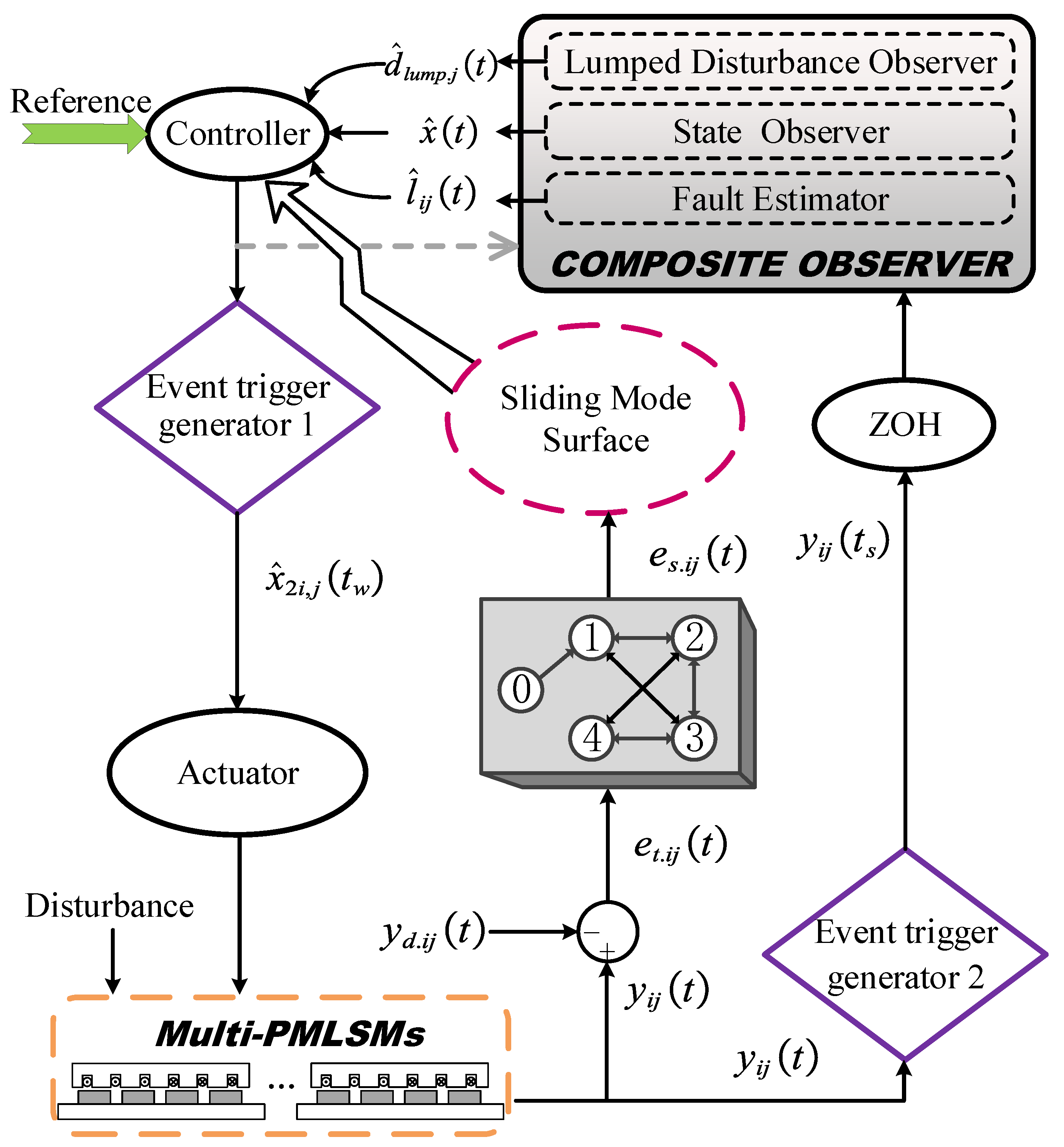
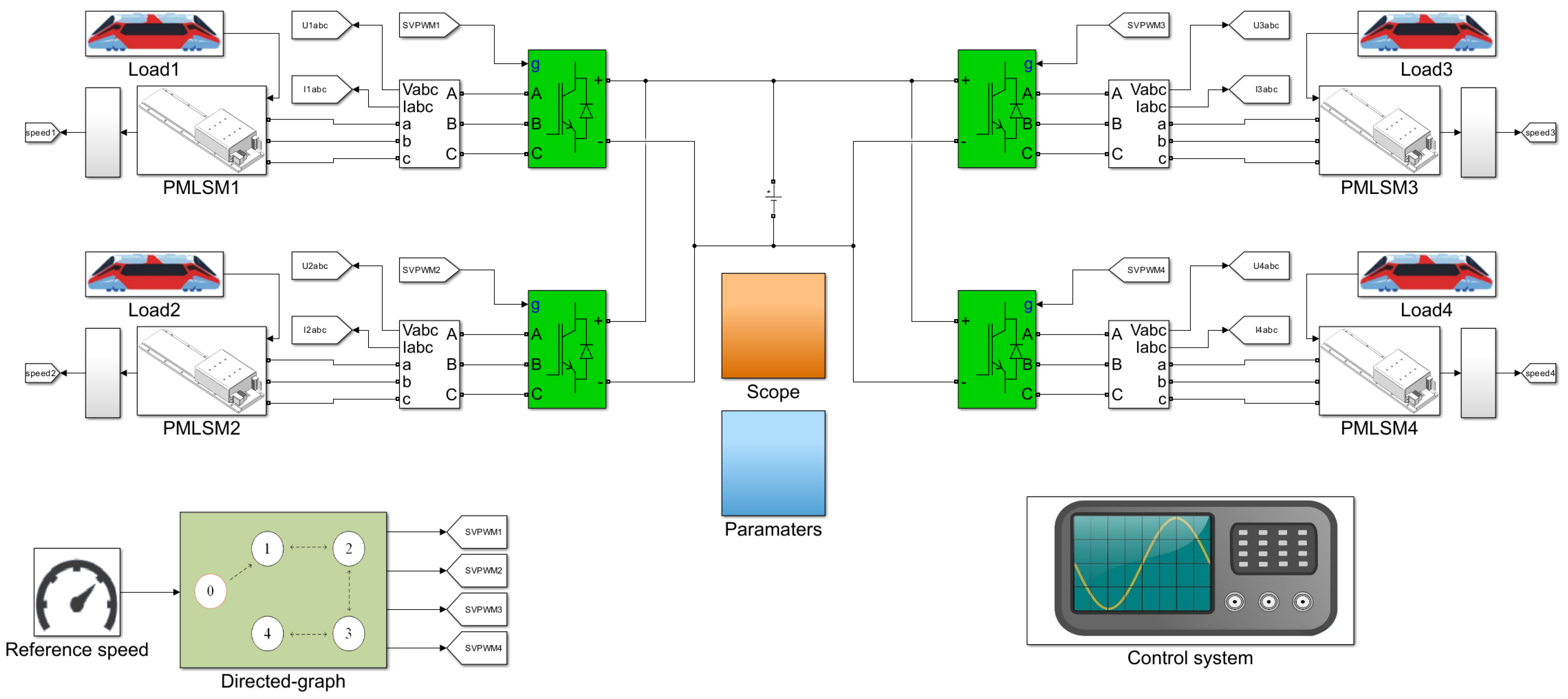
In this section, the performance of the proposed method is validated through simulation analysis. A four-motor system is constructed to employ the proposed control method, and the control diagram is depicted in Figure 3. In order to verify the effectiveness and superiority of the proposed method, this paper includes a comparison with a fuzzy-logic control (FLC) method, a field-oriented control (FOC) method, and an active disturbance rejection control (ADRC) method; the performance of the four control methods is comparatively analyzed through the MATLAB/Simulink platform. The simulation block diagram is shown in Figure 4.

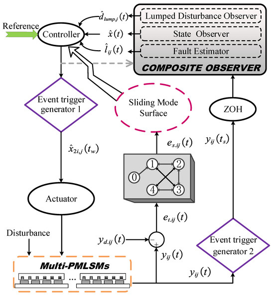
Figure 3. Control diagram of proposed method.

Figure 4. Simulation block diagram.

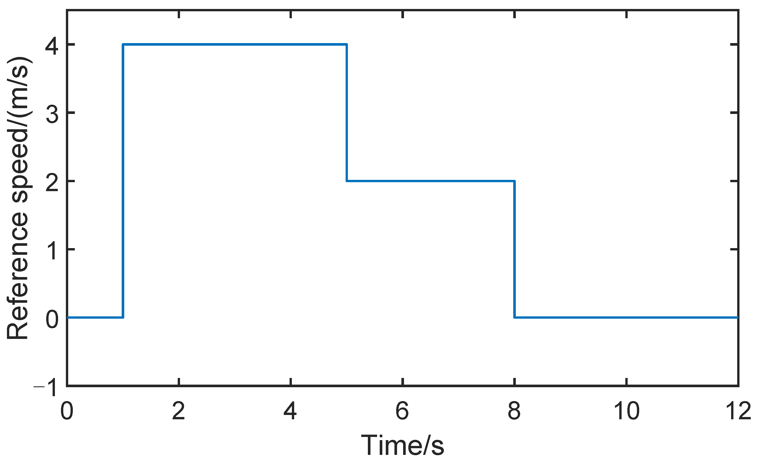
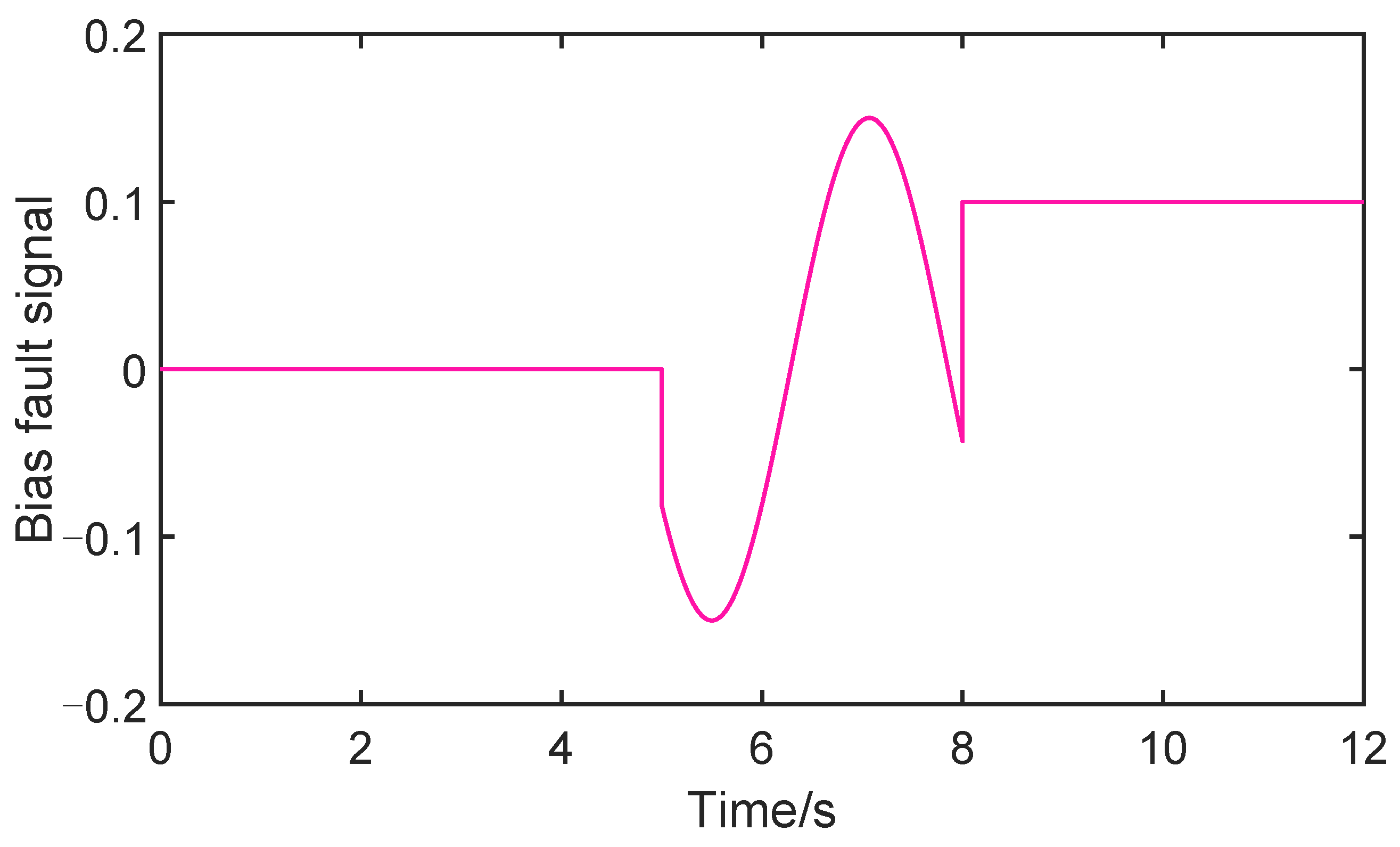
The main initial configuration parameters of the simulation are given as follows: $W=\mathrm{diag}(2,2)$, $\mathit{A}=\left[\begin{array}{cccc}0& 1& 0& 0\\ 1& 0& 1& 0\\ 0& 1& 0& 1\\ 0& 0& 1& 0\end{array}\right]$, $\mathit{B}=\mathrm{diag}(1,0,0,0)$. The tracking reference speeds of the four motors are shown in Figure 5. The disturbance is set as $d_{41}(t)=0.2sin(3t)$, $d_{42}(t)=0.2sin(3t+{\displaystyle \frac{\pi }{4}})$, $d_{43}(t)=0.2sin(3t+{\displaystyle \frac{\pi }{2}})$, and $d_{44}(t)=0.2sin(3t+{\displaystyle \frac{3\pi }{4}})$, and the system uncertainty is $u_{s.2j}(x,t)=0.001x_2^2$, $u_{s.4j}(x,t)=0.1x_{4}cos(3t)$, and $u_{s.6j}(x,t)=0.1x_{6}cos(3t)$; the bias fault is defined as

$$u_{bi}=\left\{\begin{array}{cc}0& (0\le t<5)\\ 0.15sin(2t)& (5\le t<8)\\ 0.1& (8\le t<12)\end{array}\right.$$

which can be plotted as Figure 6.

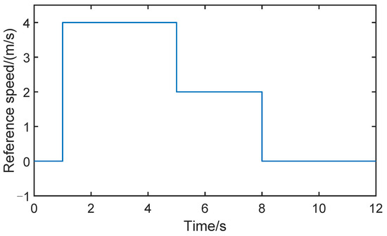
Figure 5. The reference speed in simulation.

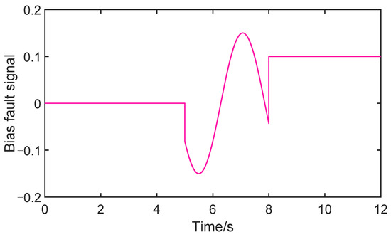
Figure 6. Bias fault signal in simulation.

Other relative parameters are shown in Table 1 and Table 2:

Table 1. Parameters of the linear motor system.

Parameters	Value	Parameters	Value
$R_s$	0.071 $\mathsf{\Omega }$	$L_d$	0.0038 H
$R_r$	0.131 $\mathsf{\Omega }$	$L_q$	0.0044 H
M	351.745 kg	${\varphi }_{pm}$	0.333 Wb
B	41.01 kg/s	$K_f$	97.5 N/A

Table 2. Parameters of the control system.

Parameters	Value	Parameters	Value	Parameters	Value
$v_a$	0.01	$v_b$	0.1	$v_c$	0.3
$k_a$	3	$k_b$	4.5	$k_c$	0.49
$a_p$	12	$n_p$	0.98	$z_e$	0.9
$k_p$	0.015	$k_r$	0.55	$l_i$	0.88

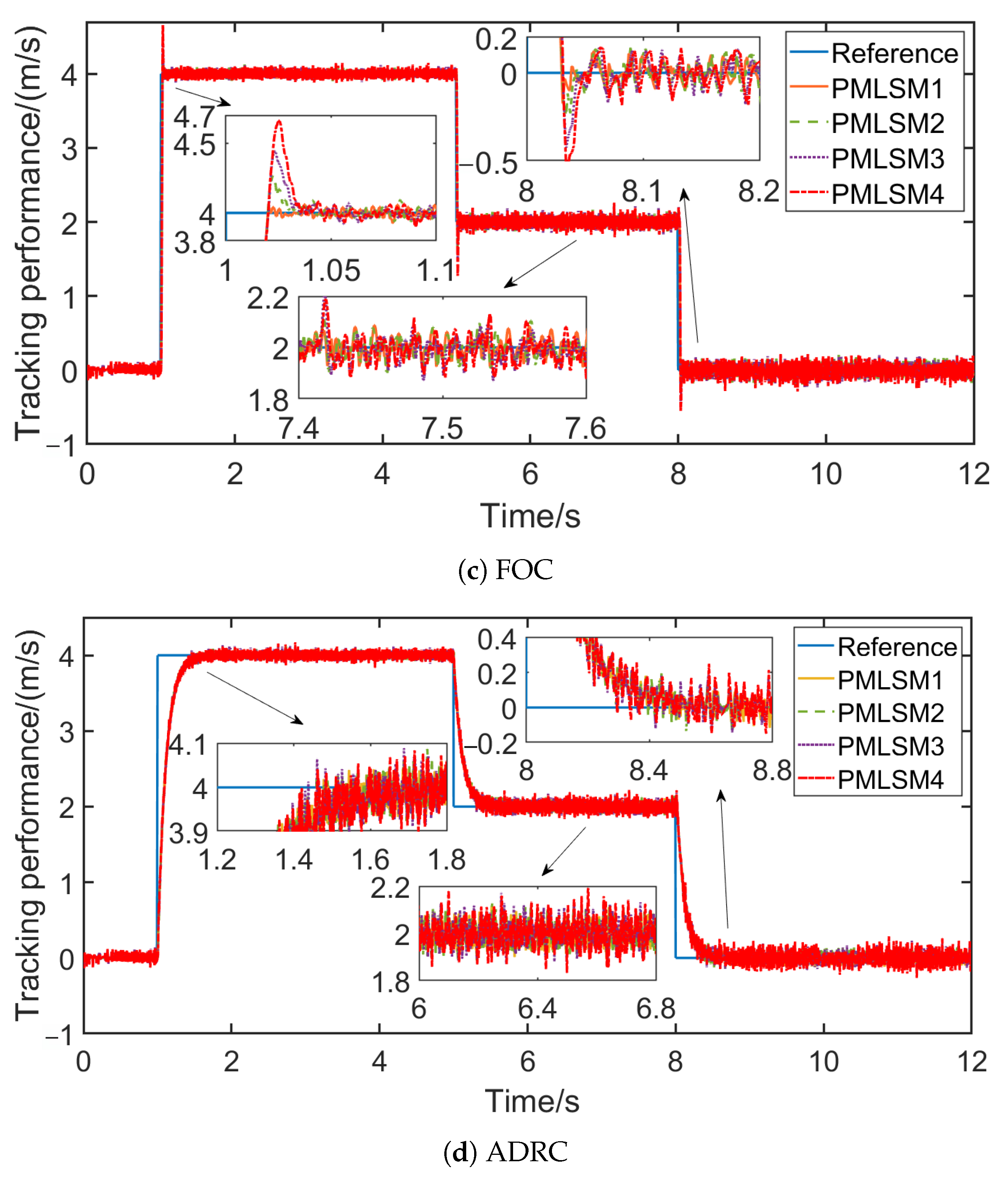
Figure 7 shows the tracking performance under the four control methods, respectively. In Figure 7a, the tracking error is suppressed to within 0.1 m/s with the proposed control method, which is superior to 0.4 m/s in Figure 7b, 0.2 m/s in Figure 7c, and 0.2 m/s in Figure 7d. As for the moments when there is an abrupt change in the reference speed, the proposed control method has a smaller magnitude of overshooting compared with FLC, FOC, and ADRC method in Figure 7b–d. Furthermore, during steady state operation, the ripple waves of the system are markedly reduced under the proposed control method.

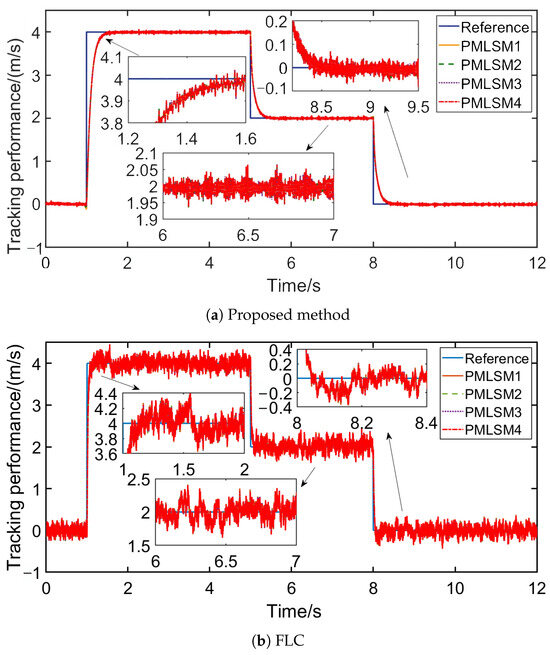
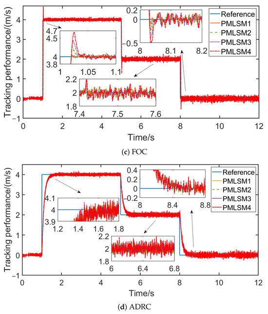
Figure 7. Tracking performance of the proposed method (a), FLC (b), FOC (c), and ADRC (d).

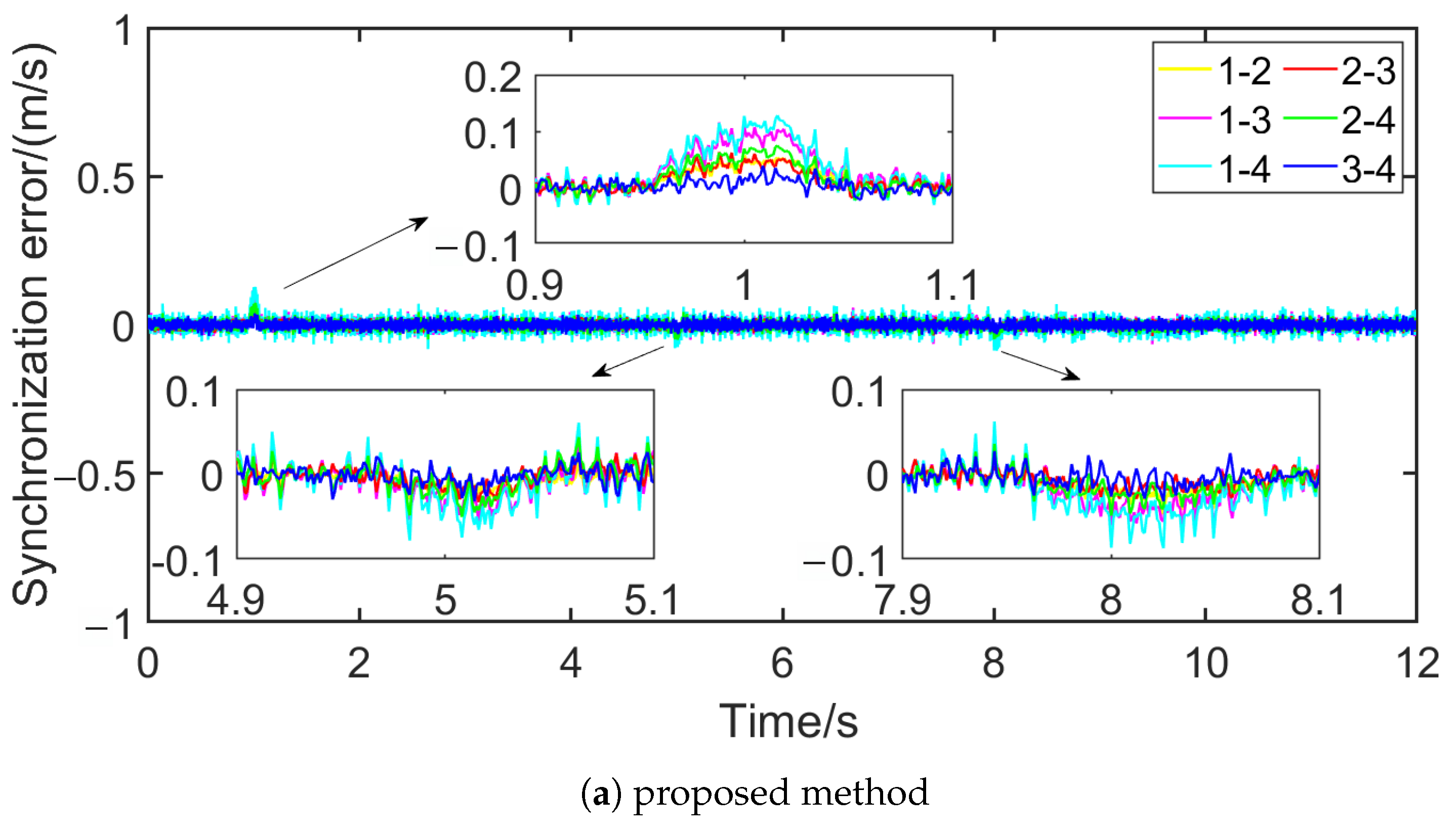
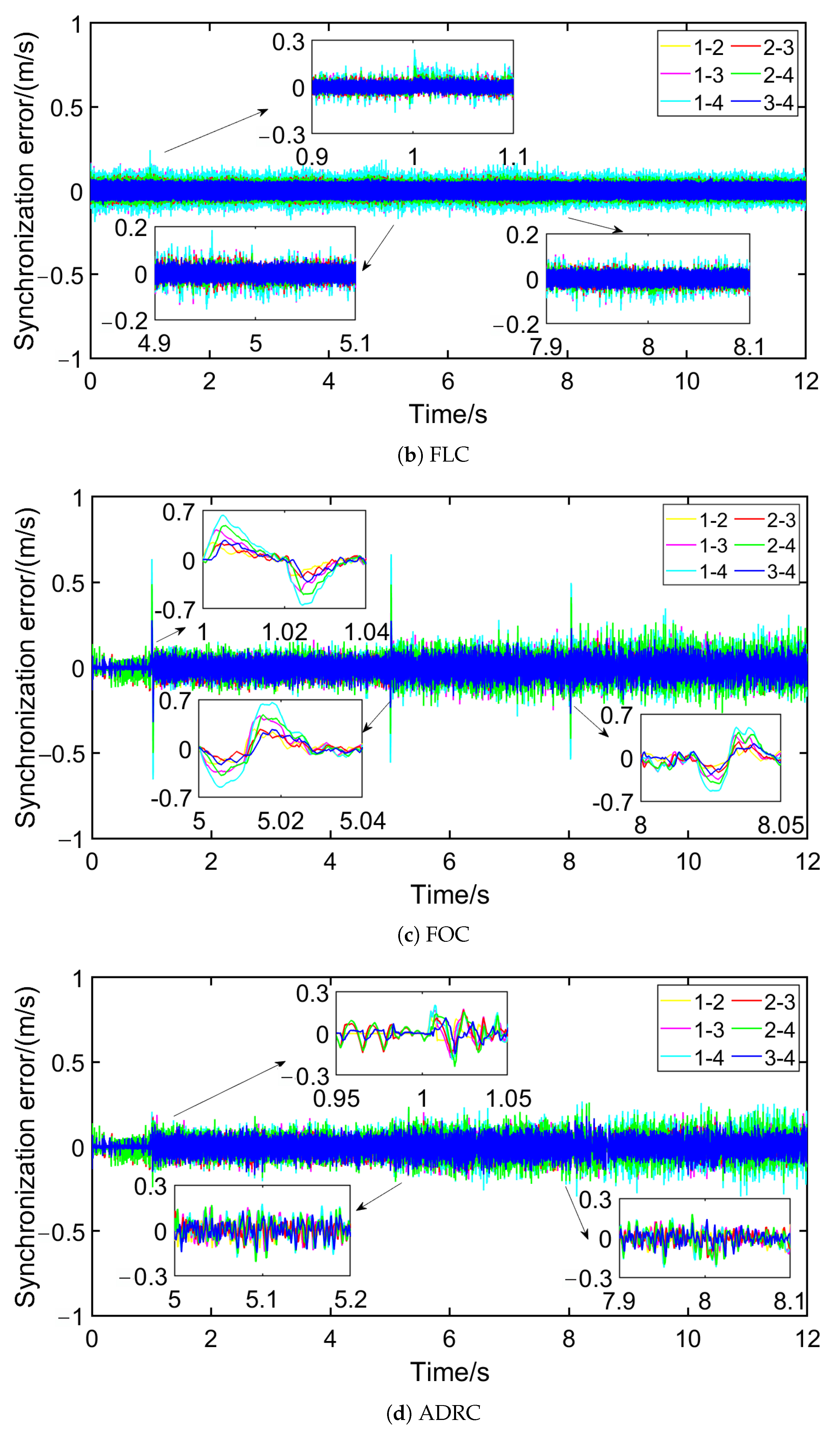
Figure 8 shows the synchronization error of each PMLSM. It is evident in Figure 8a that the synchronization error is consistently maintained below 0.1 m/s except the moments when the reference changes abruptly. Compared with Figure 8b–d, the synchronization error under the comparative control method performs poorly and cannot be maintained in a lower range, especially in Figure 8c where there are high peaks. In addition, Table 3 demonstrates the integral time absolute error under each of the above methods. It is also clear from Table 3 that the proposed method has the smallest synchronization error compared to the other methods.

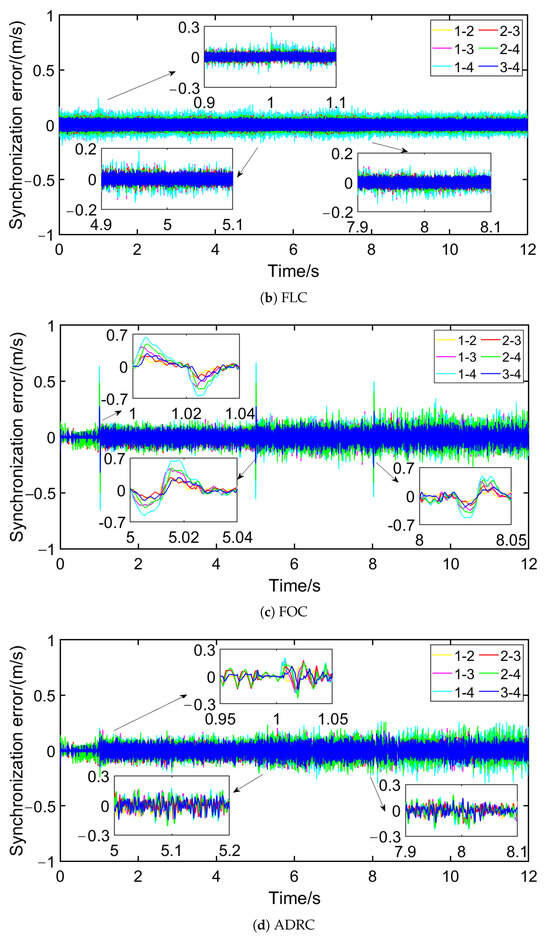
Figure 8. Synchronization error of the proposed method (a), FLC (b), FOC (c), and ADRC (d).

Table 3. Integral time absolute error of each method.

ITAE	Proposed	FLC	FOC	ADRC
1–2	0.0600	0.2348	0.3062	0.2734
1–3	0.1319	0.3348	0.5345	0.5002
1–4	0.1465	0.3668	0.6238	0.5765
2–3	0.0822	0.2281	0.4033	0.3674
2–4	0.0980	0.2395	0.5495	0.5123
3–4	0.0971	0.2070	0.4024	0.3778
SUM	0.6157	1.6110	2.8197	2.6076

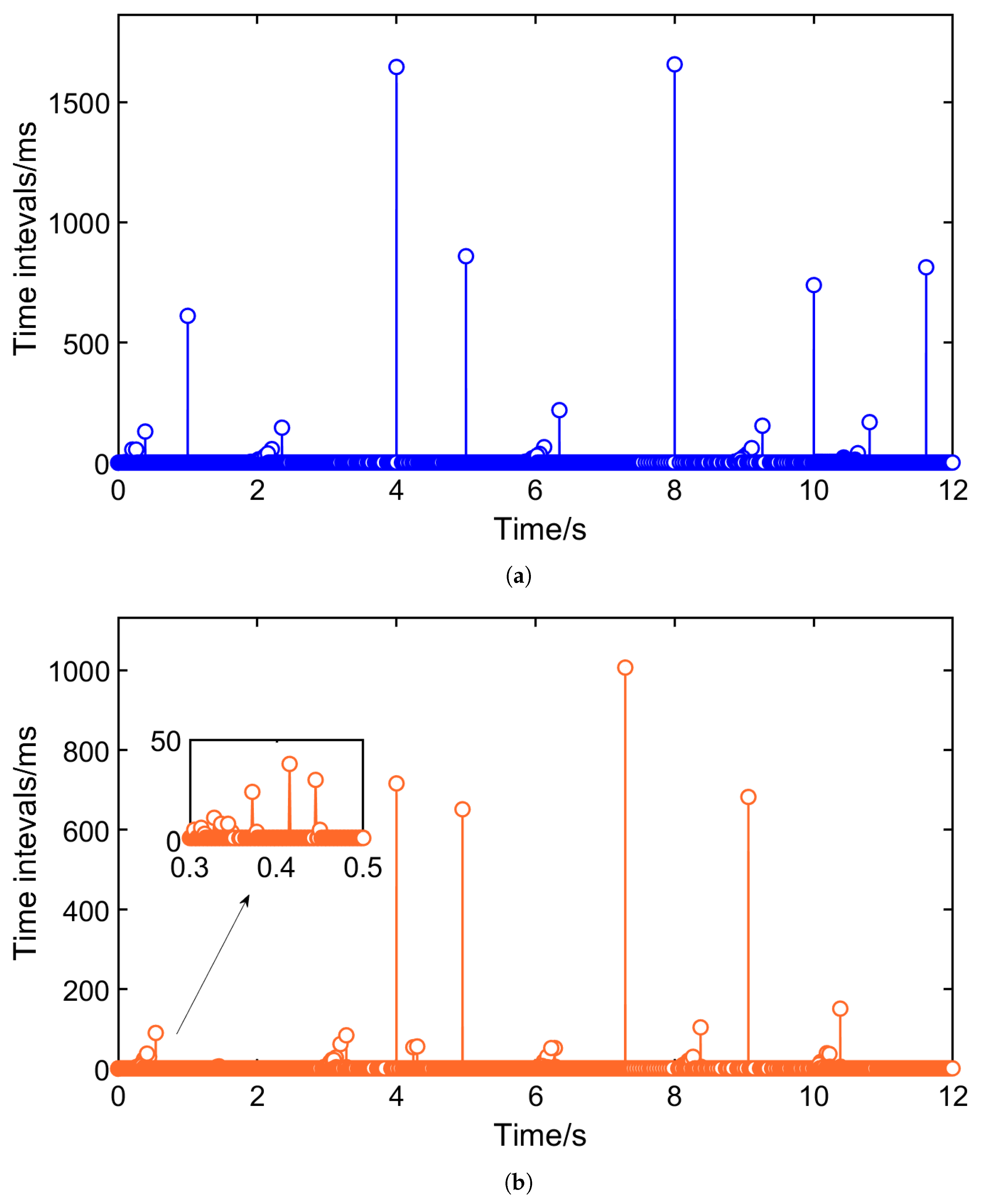
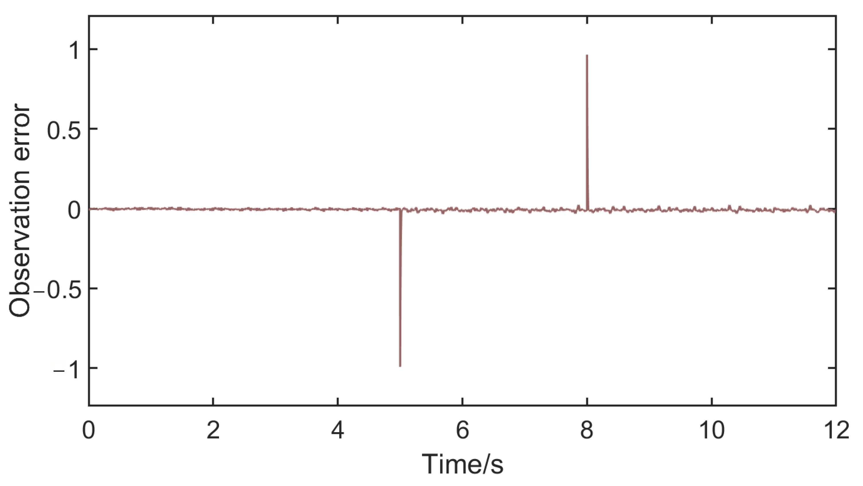
Figure 9 illustrates the event-trigger interval of both the event-trigger generators. It can be noticed that there are intervals between the triggering instances from time to time, which can be inferred as the communication burden being reduced. Furthermore, Figure 10 illustrates the observation error $e_{21}$ under the method proposed in this paper, which has a value of approximately zero, except at moments of abrupt speed changes after the fault occurs. Figure 9 and Figure 10 indicate that the control method proposed in this paper not only achieves satisfactory tracking performance but also reduces the number of triggers and alleviates the communication burden.

Figure 9. Time intervals of the event-trigger generators 1 and 2, (a) shows the intervals for generator 1, and (b) shows the intervals for generator 2.

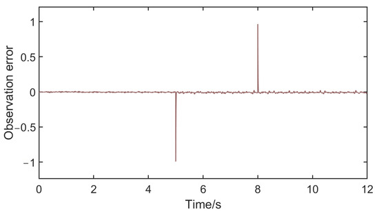
Figure 10. Observation error of the proposed method.

5. Conclusions

This paper delves into the speed tracking problem with lumped disturbances and actuator faults within an urban rail transit multi-PMLSM system. Initially, an event-triggered control scheme is constructed, where a composite observer is included. Then, a novel SMC scheme is devised based on the proposed observer. The effectiveness and superiority of the method is further demonstrated through simulation analysis. Simultaneously, the existence of Zeno behavior is falsified to ensure the practicality of the method. Finally, the method achieved an efficient, energy-saving, and high-precision cooperative fault-tolerant control of a multi-PMLSM system. Simulation results show that the tracking error under the control strategy proposed in this paper is kept below 0.1m/s, which is reduced by 0.1–0.3 m/s compared with the remaining three methods; the integral time absolute error of synchronization error is 0.6157, which is reduced by 0.9953–2.2040 compared with the remaining three methods. Through simulation analysis, the following conclusions are drawn:

• The composite observer effectively estimates lumped disturbances, which include external disturbances. This enables the adaptive sliding mode controller to compensate for these disturbances and maintain high tracking accuracy under actuator stuck faults and bias faults.
• The event-triggered mechanism reduces the communication burden by transmitting control signals only when necessary, while ensuring that Zeno behavior is avoided. This makes the method suitable for high-density urban rail networks with limited communication resources.
• The proposed method demonstrates promising application prospects in modern urban rail systems. For instance, the energy-saving performance of PMLSMs, combined with the event-triggered mechanism, can reduce energy consumption contributing to the development of low-carbon transit networks.

References

- Song, L.; Zhang, J.; Liu, Q.; Zhang, L.; Wu, X. Characteristics of Noise Caused by Trains Passing on Urban Rail Transit Viaducts. Sustainability 2025, 17, 94. [Google Scholar] [CrossRef]
- Liu, X.; Dabiri, A.; Wang, Y.; Schutter, B.D. Modeling and Efficient Passenger-Oriented Control for Urban Rail Transit Networks. IEEE Trans. Intell. Transp. Syst. 2023, 24, 3325–3338. [Google Scholar] [CrossRef]
- Chen, Z.; Liang, Y.; Tian, T.; Peng, P. Sustainable Transportation: Exploring the Node Importance Evolution of Rail Transit Networks during Peak Hours. Sustainability 2024, 16, 6726. [Google Scholar] [CrossRef]
- Zhu, L.; Chen, C.; Wang, H.; Yu, F.R.; Tang, T. Machine Learning in Urban Rail Transit Systems: A Survey. IEEE Trans. Intell. Transp. Syst. 2023, 25, 2182–2207. [Google Scholar] [CrossRef]
- Shen, X.; Wei, H.; Lie, T.T. Management and Utilization of Urban Rail Transit Regenerative Braking Energy Based on the Bypass DC Loop. IEEE Trans. Transp. Electrif. 2021, 7, 1699–1711. [Google Scholar] [CrossRef]
- Huang, Y.; Gao, X.; Song, Z.; Liu, X.; Liu, C. A Novel Wireless Motor Based on Three-Phase Six-Stator-Winding PMSM. IEEE Trans. Ind. Electron. 2024, 71, 7590–7598. [Google Scholar] [CrossRef]
- Dai, Y.; Zhang, L.; Xu, D.; Chen, Q.; Yan, X.-G. Anti-Disturbance Cooperative Fuzzy Tracking Control of Multi-PMSMs Low-Speed Urban Rail Traction Systems. IEEE Trans. Transp. Electrif. 2024, 8, 1040–1052. [Google Scholar] [CrossRef]
- Wang, D.; Peng, C.; Li, J.; Wang, C. Comparison and Experimental Verification of Different Approaches to Suppress Torque Ripple and Vibrations of Interior Permanent Magnet Synchronous Motor for EV. IEEE Trans. Ind. Electron. 2023, 70, 2209–2220. [Google Scholar] [CrossRef]
- Zhou, X.; Li, H.; Wang, L.; Peng, C.; Wang, S.; Liang, L.; Deng, Z. Vertical Dynamic Response Analysis of HTS Maglev Vehicle Excited by a Designed Coreless-Typed PMLSM. IEEE Trans. Transp. Electrif. 2023, 9, 3421–3433. [Google Scholar] [CrossRef]
- Zhang, G.; Zhang, H.; Li, B.; Wang, Q.; Ding, D.; Wang, G.; Xu, D. Auxiliary Model Compensated RESO-Based Proportional Resonant Thrust Ripple Suppression for PMLSM Drives. IEEE Trans. Transp. Electrif. 2023, 9, 2141–2152. [Google Scholar] [CrossRef]
- Dong, F.; Zhao, J.; Zhao, J.; Song, J.; Chen, J.; Zheng, Z. Robust Optimization of PMLSM Based on a New Filled Function Algorithm With a Sigma Level Stability Convergence Criterion. IEEE Trans. Ind. Inform. 2021, 17, 4743–4754. [Google Scholar] [CrossRef]
- Xu, W.; Liao, K.; Ge, J.; Qu, G.; Cheng, S.; Wang, A.; Boldea, I. Improved Position Sensorless Control for PMLSM via an Active Disturbance Rejection Controller and an Adaptive Full-Order Observer. IEEE Trans. Ind. Appl. 2023, 59, 1742–1753. [Google Scholar] [CrossRef]
- Xiang, B.; Wen, T.; Liu, H. Cooperative Control of Multiple PM Actuators in PMLSM With Segmented Windings. IEEE Trans. Transp. Electrif. 2024, 10, 5570–5580. [Google Scholar] [CrossRef]
- Song, H.; Gao, S.; Li, Y.; Liu, L.; Dong, H. Train-Centric Communication Based Autonomous Train Control System. IEEE Trans. Intell. Veh. 2023, 8, 721–731. [Google Scholar] [CrossRef]
- Wang, X.; Li, S.; Tang, T.; Yang, L. Event-Triggered Predictive Control for Automatic Train Regulation and Passenger Flow in Metro Rail Systems. IEEE Trans. Intell. Transp. Syst. 2022, 23, 1782–1795. [Google Scholar] [CrossRef]
- Xu, D.; Huang, J.; Su, X.; Shi, P. Adaptive command-filtered fuzzy backstepping control for linear induction motor with unknown end effect. Inf. Sci. 2019, 477, 118–131. [Google Scholar] [CrossRef]
- Hu, D.; Xu, W.; Dian, R.; Liu, Y.; Zhu, J. Loss minimization control of linear induction motor drive for linear metros. IEEE Trans. Ind. Electron. 2018, 65, 6870–6880. [Google Scholar] [CrossRef]
- Li, H.; Sheng, H.; Shen, L. Iterative learning PID controller for permanent magnet linear synchronous motor. J. Phys. Conf. Ser. 2021, 1852, 032044. [Google Scholar] [CrossRef]
- Li, L.; Cheung, N.; Yang, G.; Wang, C.; Fu, P.F.; Li, G.C.; Pan, J.F. Design of a variable-gain adjacent cross-coupled controller for coordinated motion of multiple permanent magnet linear synchronous motors. Comput. Electron. Agric. 2022, 192, 106561. [Google Scholar] [CrossRef]
- Zhu, H.; Shi, L.; Zhang, M. A Novel Thrust Control Based on Total Resistance Force Observation for Long Primary Linear Induction Motor. In Proceedings of the 2021 24th International Conference on Electrical Machines and Systems (ICEMS), Gyeongju, Republic of Korea, 31 October–3 November 2021; pp. 1798–1801. [Google Scholar]
- Pan, J.; Fu, P.; Niu, S.; Wang, C.; Zhang, X. High-Precision Coordinated Position Control of Integrated Permanent Magnet Synchronous Linear Motor Stations. IEEE Access 2020, 8, 126253–126265. [Google Scholar] [CrossRef]
- Fu, P.; Pan, J.; Wang, C.; Huang, R. Research on Coordinated Control of Multi-PMSLM Based on Sliding Mode Variable Structure Deviation Coupling Algorithm. In Proceedings of the 2019 22nd International Conference on Electrical Machines and Systems (ICEMS), Harbin, China, 11–14 August 2019; pp. 1–5. [Google Scholar]
- Mao, Z.; Yan, X.-G.; Jiang, B.; Chen, M. Adaptive Fault-Tolerant Sliding-Mode Control for High-Speed Trains With Actuator Faults and Uncertainties. IEEE Trans. Intell. Transp. Syst. 2020, 21, 2449–2460. [Google Scholar] [CrossRef]
- Guo, Y.; Wang, Q.; Sun, P.; Feng, X. Distributed Adaptive Fault-Tolerant Control for High-Speed Trains Using Multi-Agent System Model. IEEE Trans. Veh. Technol. 2020, 73, 3277–3286. [Google Scholar] [CrossRef]
- Shi, P.; Wang, X.; Meng, X.; He, M.; Mao, Y.; Wang, Z. Adaptive Fault-Tolerant Control for Open-Circuit Faults in Dual Three-Phase PMSM Drives. IEEE Trans. Power Electron. 2023, 38, 3676–3688. [Google Scholar] [CrossRef]
- Zhang, Z.; Chen, Z. Fault Estimation and Tolerant Control of a Class of Nonlinear Systems and Its Application in High-Speed Trains. IEEE Trans. Control. Syst. Technol. 2023, 31, 2903–2911. [Google Scholar] [CrossRef]
- Lin, X.; Bai, W.; Wang, Q.; Yu, S. Virtual Coupling-Based H Active Fault-Tolerant Cooperative Control for Multiple High-Speed Trains With Unknown Parameters and Actuator Faults. IEEE J. Emerg. Sel. Top. Circuits Syst. 2023, 13, 780–788. [Google Scholar] [CrossRef]
- Zheng, J.; Hou, Z. Model Free Adaptive Iterative Learning Control Based Fault-Tolerant Control for Subway Train With Speed Sensor Fault and Over-Speed Protection. IEEE Trans. Autom. Sci. Eng. 2024, 21, 168–180. [Google Scholar] [CrossRef]
- Guo, X.; Wei, G.; Ding, D. Fault-Tolerant Consensus Control for Discrete-Time Multi-Agent Systems: A Distributed Adaptive Sliding-Mode Scheme. IEEE Trans. Circuits Syst. II Express Briefs 2023, 70, 2515–2519. [Google Scholar] [CrossRef]
- Yu, W.; Huang, D.; Wang, Q.; Cai, L. Distributed Event-Triggered Iterative Learning Control for Multiple High-Speed Trains With Switching Topologies: A Data-Driven Approach. IEEE Trans. Intell. Transp. Syst. 2023, 24, 10818–10829. [Google Scholar] [CrossRef]
- Bai, W.; Dong, H.; Lü, J.; Li, Y. Event-Triggering Communication Based Distributed Coordinated Control of Multiple High-Speed Trains. IEEE Trans. Veh. Technol. 2021, 70, 8556–8566. [Google Scholar] [CrossRef]
- Wang, J.; Pan, H.; Sun, W. Event-Triggered Adaptive Fault-Tolerant Control for Unknown Nonlinear Systems With Applications to Linear Motor. IEEE/ASME Trans. Mechatron. 2022, 27, 940–949. [Google Scholar] [CrossRef]
- Wang, J.; Ma, J.; Pan, H.; Sun, W. Event-Triggered Adaptive Saturated Fault-Tolerant Control for Unknown Nonlinear Systems With Full State Constraints. IEEE Trans. Autom. Sci. Eng. 2024, 21, 1837–1849. [Google Scholar] [CrossRef]
- Zhao, X.M.; Gong, Y.W.; Jin, H.Y.; Xu, C. Adaptive super-twisting-based nonsingular fast terminal sliding mode control of permanent magnet linear synchronous motor. Trans. Inst. Meas. Control. 2023, 45, 3057–3066. [Google Scholar] [CrossRef]
- Xu, D.; Zhang, W.; Shi, P.; Jiang, B. Model-Free cooperative adaptive sliding-mode-constrained-control for multiple linear induction traction systems. IEEE Trans. Cybern. 2020, 50, 4076–4086. [Google Scholar] [CrossRef]
Disclaimer/Publisher’s Note: The statements, opinions and data contained in all publications are solely those of the individual author(s) and contributor(s) and not of MDPI and/or the editor(s). MDPI and/or the editor(s) disclaim responsibility for any injury to people or property resulting from any ideas, methods, instructions or products referred to in the content. |
© 2025 by the authors. Licensee MDPI, Basel, Switzerland. This article is an open access article distributed under the terms and conditions of the Creative Commons Attribution (CC BY) license (https://creativecommons.org/licenses/by/4.0/).