Abstract
Understanding the impacts of land use/land cover (LULC) changes on ecological processes is essential for addressing biodiversity loss, habitat fragmentation, and climate change. This study analyzes the effects of LULC changes on habitat quality and landscape connectivity in İzmir, Turkey’s third-largest city, using the Integrated Valuation of Ecosystem Services and Trade-offs Habitat Quality (InVEST HQ) model, Conefor 2.6 connectivity analysis, and Circuitscape 4.0 resistance-based modeling. This study relies on Coordination of Information on the Environment (CORINE) Land Cover data from 1990 to 2018. Findings indicate that artificial surfaces increased by 82.5% (from 19,418 ha in 1990 to 35,443 ha in 2018), primarily replacing agricultural land (11,721 ha converted). Despite this expansion, high quality habitat areas remained relatively stable, though habitat fragmentation intensified, with the number of patches rising from 469 in 1990 to 606 in 2018, and the average patch size decreasing from 394.31 ha to 297.39 ha. Connectivity analysis highlighted Mount Nif and the Urla–Çeşme–Karaburun Peninsula as critical ecological corridors. However, resistance to movement increased, reducing the likelihood of connectivity-supporting corridors. These findings emphasize the importance of integrating spatial modeling approaches into urban planning and conservation strategies to mitigate future habitat loss and fragmentation.
1. Introduction
Studies have shown that land use/land cover (LULC) changes due to urbanization, agriculture, and other anthropogenic activities lead to significant declines in habitat quality, with profound impacts on biodiversity and ecological functioning and ecosystem services [1,2,3]. Therefore, research to understand the relationships between LULC changes and habitat quality has become an important topic in recent years, especially in the field of ecology. In rapidly urbanizing areas, urban expansion has been identified as a critical factor contributing to habitat degradation [4,5], showing that the proximity of urban areas to natural habitats can significantly alter their ecological function and structure [6]. Furthermore, Li et al. (2022) underlined that future urban expansion may lead to long-term ecological changes by impacting terrestrial vertebrate habitats [7]. The relationship between LULC changes and habitat quality is not limited to urbanization but also includes agricultural practices. Ding et al. (2021) noted that agricultural expansion generally leads to a decline in habitat quality, but some studies have suggested that certain agricultural practices can improve habitat quality under certain conditions [8]. Kija et al. (2020) reported that human population growth and agricultural expansion in the Greater Serengeti Ecosystem has led to significant habitat degradation, resulting in a high proportion of low-quality habitat [9]. This trend is echoed in the findings of Ge et al. (2023) who noted that human activities, including overgrazing and deforestation, have a detrimental impact on habitat quality, while ecological restoration efforts can improve it [10]. Furthermore, research by Zheng and Li (2022) emphasized that changes in LULC structure and intensity profoundly affect the flow of materials and energy between habitat patches, thereby affecting regional habitat quality [11]. Ongoing research in this area underscores the urgent need for sustainable land management practices that balance human development with ecological conservation [12]. Quantifying and monitoring the effects of LULC changes on habitat quality is considered essential for the effective conservation and management of ecosystems [13,14].
In response to this growing need, various studies have attempted to assess habitat quality through different methodological approaches [15]. These assessments generally rely on two primary methodologies: field surveys and modeling techniques. Field surveys, which involve direct observation and data collection from specific locations within a habitat [3,16], provide detailed ecological information, such as habitat selection, abundance, diversity, and demographics of species [17,18], which is critical for understanding the habitat quality needs of species and for targeted conservation efforts [19,20]. It can also capture the complexity of species’ habitat requirements and ecological interactions, which allows for a more comprehensive assessment of habitat quality [21,22,23]. However, the results of field studies can be influenced by the expertise and biases of observers, potentially leading to inconsistencies in data interpretation [24]. Furthermore, due to the relatively high cost of data collection, the application of the method is often limited to small areas and short time scales, making it difficult to monitor the dynamics of different types of habitat conditions in different areas [25,26,27].
While field-based methods provide high-resolution ecological data, their limitations in spatial and temporal coverage highlight the need for scalable and adaptive assessment approaches. Given the increasing challenges posed by habitat loss and fragmentation due to LULC changes, researchers have increasingly turned to modeling techniques to analyze habitat quality at broader scales. These approaches allow for the integration of diverse data sources and provide a more comprehensive understanding of habitat quality dynamics, facilitating their application in ecosystem management and conservation planning [28,29]. In addition, habitat quality dynamics, which are considered to be an important indicator in ensuring the continuity of ecosystem services, including flood regulation, water purification, and carbon sequestration, which are critical in ensuring resilience against current environmental problems, such as climate change and biodiversity loss, need to be examined, monitored, and evaluated at different spatial and temporal scales [30,31,32]. Ecological process models, which are a simplified version of ecological processes, have been widely used in recent years due to the insight they provide into the threat of human activities to habitat quality. Capable of analyzing large geographical areas, these modeling approaches are suitable for regional or global assessments [16], and their scalable nature makes them particularly useful for understanding the impacts of urbanization and LULC changes on habitat quality [1]. Although the accuracy of their results is highly dependent on the quality of the input data [3] and they risk not fully capturing the complexity of ecological systems due to their simplification of real-world conditions [33,34], they have become frequently used tools for assessing and mapping habitat quality at large spatial scales [35,36,37,38], monitoring habitat quality dynamics [39,40], and identifying areas vulnerable to habitat degradation [41]. Habitat quality is a critical factor in conservation and restoration efforts as it directly affects biodiversity and ecosystem health. Numerous studies have focused on identifying areas of high habitat quality and understanding the dynamics affecting these habitats [42,43,44].
Notable among these studies are those that examine the links between areas of high habitat quality. Habitat fragmentation often results in isolated patches that hinder the dispersal of species and thus threaten their survival [22,23]. Connectivity between habitats improves ecological functioning by securing the flow of energy, species, and matter [45,46,47], and connected habitats support higher levels of biodiversity and ecosystem functioning than isolated patches [48,49]. Research shows that effective conservation strategies should prioritize the identification of ecological corridors and stepping stone habitats that increase connectivity between high-quality habitats [41,50,51]. However, to improve the efficiency of monitoring and conservation efforts, it is crucial to develop robust quantitative methods that can indicate which key areas and landscape elements play important and critical roles in the functioning of habitat mosaics [52].
Despite extensive research on the relationship between LULC changes—driven by urbanization, agricultural expansion, and other anthropogenic activities—and habitat quality and connectivity, a critical gap remains in assessing their long-term impacts using an integrated geospatial modeling approach. This study addresses this gap by combining multiple spatial analysis techniques to evaluate habitat quality and connectivity shifts in rapidly urbanizing Mediterranean landscapes. Focusing on İzmir, this study examines LULC changes between 1990 and 2018 to answer three key questions: (1) How have LULC changes influenced habitat quality over the past three decades? (2) To what extent has urban expansion altered landscape connectivity? (3) How can spatial modeling enhance habitat quality and connectivity assessments? İzmir, a rapidly urbanizing Mediterranean coastal city, has undergone major LULC transformations since the 1980s [53,54] affecting ecologically significant areas, such as the Gediz Delta Wetlands, Mount Yamanlar, the Bozdağlar Mountains, and the Menderes Basin [55,56], while also facing climate change-related challenges, like rising temperatures, drought, and coastal erosion. These pressures have heightened the need to integrate ecological restoration and nature-based solutions into urban planning, emphasizing the growing demand for robust scientific data to ensure their effective implementation [57,58].
Aligned with the UN 2030 Sustainable Development Goals (SDGs), this study contributes to Goal 15 (biodiversity conservation), Goal 13 (climate resilience), and Goal 11 (sustainable urbanization). It prioritizes large-scale, reliable, and accessible data sources to support decision-making for global environmental challenges. The European Coordination of Information on the Environment (CORINE) Land Cover dataset was selected as the primary data source. Habitat quality was assessed using the Integrated Valuation of Ecosystem Services and Trade-offs Habitat Quality (InVEST HQ) model, while Conefor 2.6 identified critical habitats for conservation and sustainable landscape management. Circuitscape 4.0 was utilized to model ecological corridors and connectivity pathways.
2. Materials and Methods
2.1. Study Area
The case study area includes 11 central districts in İzmir (Balçova, Bayraklı, Bornova, Buca, Çiğli, Gaziemir, Güzelbahçe, Karabağlar, Karşıyaka, Konak, and Narlıdere), Turkey’s third-largest city in terms of population, where LULC changes caused by the metropolitan area are prominent. It also encompasses the districts of Menemen, Torbalı, Kemalpaşa, and Urla, which are located along the city’s development axis. The total surface area of the study area is 3489.02 km2 and the population has increased from 2,694,770 in 1990 to 4,320,519 in 2024. Located on the Aegean Sea coast in western Turkey (Figure 1) [59,60], the study area has a Mediterranean climate characterized by hot–dry summers and mild–wet winters [61]. Annual rainfall varies between 300 mm and 700 mm [62]. The vegetation in the study area is dominated by typical Mediterranean flora [63]. The geography of the region combines different landforms and geomorphological features, such as mountainous, rugged landscapes, caves, islands, lakes, and wetlands, which supports its richness in terms of natural landscapes, species, and vegetation [53].
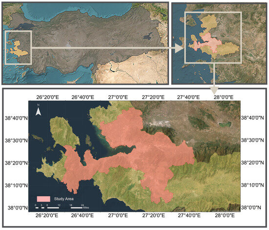
Figure 1.
Location of the study area.
As a result of urban sprawl in parallel with rapid population growth and economic development, valuable agricultural land and natural habitats have been converted to residential, commercial, and industrial uses. The available evidence suggests that İzmir has experienced significant changes in its agricultural pattern and natural landscapes, such as forests, maquis and frigana, since the 1990s [64,65,66]. These changes, driven by urbanization policies, economic factors, growing population needs, and environmental constraints, have led to landscape fragmentation and reduced habitat connectivity. In recent years, planning efforts focused on ensuring İzmir’s ecological security and resilience have gained momentum [67], and approaches to supporting the natural structure have gained importance.
2.2. Methodology
The research methodology consists of four steps: (1) investigate the change in LULC of İzmir city and its surroundings between 1990, and 2000, 2006, 2012, and 2018; (2) examine the changes in habitat quality and the degree of habitat degradation in the study area; (3) determine the change of priority habitats in terms of connectivity; (4) determine the change of corridors with high connectivity probability. The data were transformed at a spatial resolution of 50 × 50 m. Although spatial changes driven by the accelerating urbanization process in the study area have been reported to increase since the 1980s [68], this study prioritizes the need for rapid information flow to support decision-making processes. Therefore, the European Commission’s CORINE Land Cover dataset, which provides accessible geospatial data, was utilized. The selected time points correspond to the available data years within this dataset.
2.2.1. LULC Change Analysis
LULC data from the CORINE Land Cover database for the years 1990, 2000, 2006, 2012, and 2018 were used to make an assessment based on homogeneous criteria to determine the change of LULC in the city of İzmir. The CORINE Land Cover nomenclature presents 44 classes of the European LULC pattern based on five main thematic groups, artificial surfaces, agricultural areas, forests and semi-natural areas, wetlands, and water bodies [69], at three hierarchical levels. CORINE Land Cover data can be used for temporal and spatial detection of LULC patterns and changes [70,71], as well as for the analysis of LULC changes on habitat quality and biodiversity [72,73,74], ecosystem services, such as water supply, carbon sequestration, and recreation [75,76], and environmental pressures and threats [77]. Within the framework of habitat characteristics, the LULC classes in the study area was evaluated within the framework of 10 classes, depending on its features and characteristics (Table 1).

Table 1.
CORINE Land Cover Level 3 content of LULC classes used in this study.
In this study, cross tabulation was used to calculate LULC changes. Cross tabulation is a widely used analytical tool for analyzing LULC changes [78]. Cross-tabulation, a statistical technique that allows analyzing the relationship between two or more categorical variables [79], provides a clear way to understand the complex nature of change by measuring changes over time between different LULC classes, and allows researchers to identify dominant change processes and their underlying drivers [80,81].
2.2.2. Assessing Habitat Quality Using InVEST HQ Model
This study used the open-source InVEST model version 3.14.2 to calculate and map habitat quality [82]. The InVEST HQ model is a crucial component for assessing the condition of natural habitats and their ability to support biodiversity [83,84]. By prioritizing the spatial structure of biodiversity, the model is based on the idea that species’ habitats can be predicted by analyzing LULC maps alongside threats to these habitats, and it evaluates habitat quality based on factors such as land use, threats, and species sensitivity to these threats [42,43,85]. It assesses habitat quality and rarity as a function of four key factors: the relative impact of each threat, the relative sensitivity of each habitat type to these threats, the distance between habitats and threat sources, and the legal protection status of the land [86].
The InVEST HQ model has been widely used in recent years due to its requirement for simple input data, ease of use [87,88], its ability to provide spatially explicit outputs that can be easily visualized and analyzed [89], its applicability across various spatial scales from local to regional and even national levels [90], and its capacity to be integrated with different assessment methods [91,92].
In this study, habitat quality values were calculated and mapped using the following equations with reference to LULC maps for 1990, 2000, 2006, 2012, and 2018;
where Qxj denotes the habitat quality index of grid x of LULC type j; Hj denotes the habitat suitability of the LULC type j, ranging from 0 to 1; Dxj is the habitat degradation degree, representing the habitat degradation degree level of grid x in land-use type j; Z is the scale constant, which is generally taken as 2.5; and K is the semi saturated constant, which is generally taken as 0.5. The value of Qxj is between 0 and 1, with Qxj values close to 0 indicating low habitat quality, and Qxj values close to 1 indicating a high habitat quality [93,94]. Habitat degradation (Dxj) was calculated using the following equation:
where Dxj represents the xth grid cell’s threat level of the jth LULC type; R is the number of stress factors; Yr is the total number of grid units of stress factors; y represents the grid cells entirety on threat r’s raster map; wr represents the weight of each threat factor, ranging from 0 to 1; ry represents the yth grid cell’s threat intensity (ranging from 0 to 1); irxy represents the distance between the habitat and the threat source; βx represents the xth grid cell’s accessibility level (ranging from 0 to 1); and Sjr represents the relative sensitivity of LULC type j to different threat factors (ranging from 0 to 1). The habitat degradation degree can range from 0 to 1, with Dxj values close to 1 indicating a high degree of habitat degradation [95].
The linear and exponential distance-decay functions between the habitat and the threat source can be expressed as Equations (3) and (4):
where dxy is the linear distance between grid x and y; drmax is the maximum operating distance of the threat r.
In the calculation of habitat quality, LULC maps consisting of 10 classes used in the change analysis were used as the main data set. In addition, continuous urban fabric, discontinuous urban fabric, agricultural areas, industrial areas, mines, and airport, obtained by reclassification of the CORINE Land Cover dataset, were also considered as threats due to their potential to pose a threat to the habitat quality of other LULC classes in the area. A dataset downloaded from the Open Street Map was used to identify major and secondary roads. Ring roads and highways were classified as major roads and intercity highways were classified as secondary roads. Urban roads were not taken into consideration.
This module requires land use, stress factors, stress sources, habitat types and sensitivity of habitat types to stress, and semi-saturation parameters in order to make calculations. In this study, the relevant parameters were determined by taking into account the existing studies in the literature, primarily in the Mediterranean region, and previous experiences for the city of İzmir [37,41,93,96] (Table 2 and Table 3).
Table 2.
Threat factors parameters.
Table 3.
Habitat suitability and sensitivity of the habitats to each threats.
2.2.3. Importance of Habitats for Connectivity
Conefor 2.6 software was used to assess the importance of patches with a high habitat quality in terms of connectivity. Conefor 2.6 allows quantification of landscape connectivity based on graph theory principles and can analyze the importance of habitat patches and corridors for maintaining overall connectivity within a landscape [97,98]. This information is crucial for prioritizing habitat protection, restoration, and management areas to ensure the long-term viability of species populations [99].
Through graph structure and habitat availability indices, Conefor 2.6 analyzes not only the spatial arrangement of habitats (structural connectivity), but functional connectivity, taking into account species range and behavioral responses [100,101]. Graph theory (landscape graphs) is an effective method for analyzing landscape patterns and allows the landscape to be represented as a network [102,103]. Through this approach, it is possible to analyze both how habitat fragments are connected to each other and how these connections affect landscape connectivity [104,105,106]. Two concepts come to the fore here: nodes and links. Nodes represent habitat fragments or suitable habitats (e.g., protected areas), while links represent the potential for species to move from one habitat area to another. Graph structures optimize large data sets and complex linkage analyses, resulting in high computational efficiency, especially in large-scale linkage analyses. Habitat accessibility indices are a comprehensive approach that assesses a habitat patch through both intrapatch connectivity and interpatch connectivity [107]. In habitat accessibility, a species’ ability to easily access its habitat depends on habitat abundance (quantity) and habitat connectivity [108]. If connectivity between habitat fragments is poor or the amount of habitat is insufficient, accessibility for species is reduced.
Unlike software such as Fragstats [109] and APACK [110], Conefor 2.6 helps to identify critical habitat elements in landscape planning and habitat conservation processes, and provides a descriptive analysis of the landscape [111]. It allows quantifying the importance of individual habitat patches for maintaining functional landscape connectivity and assessing the connectivity enhancement provided by new potential habitat areas that can be added to the landscape through habitat creation or restoration.
In this study, two complementary indices, the integral index of connectivity (IIC) and the probability of connection (PC) index, were used together to understand different connectivity mechanisms and provide a background for optimizing habitat connectivity [112,113,114]. Both indices integrate the habitat patch area (or other patch attributes) and connections between different patches in a single metric [107]. The integral index of connectivity (IIC), which assesses the connections between the habitat patches using a binary model of “present” and “absent”, considers habitats as connected or not connected according to the distance between them [115]. The probability of connectivity (PC) index evaluates the connections between habitats using a probabilistic model. The index calculates the probability of direct dispersal between two habitat patches with an exponential function that decreases with increasing distance, and the connections are weighted as the strength of the connection is assumed to change with distance [116,117]. In addition to connectivity, the delta versions of the IIC and PC indices (dPC, dIIC) are used in this study [107,118], as the aim is to reveal the importance of each patch in terms of connectivity. These indices, which can be interpreted as the percentage importance of each patch in the overall connectivity, take values between 0 and 100, with small values indicating low importance for the overall connectivity of the habitat patch network, and large values indicating high importance [119,120]. In determining the importance of patches in terms of connectivity, areas with a high habitat quality in the range of 0.6–1.0 obtained from the InVEST HQ model were used as input data.
2.2.4. Evaluation of Changes in Possible Pathways Between Habitats
In this study, the Circuitscape 4.0 modeling tool was used to analyze how connectivity between habitats has changed in response to temporal changes in the LULC. Circuitscape 4.0 is an open source software that uses electrical circuit theory for heterogeneous landscapes. It is a tool for modeling plant and animal movement and gene flow, as well as for identifying areas where connectivity needs to be preserved. By treating the landscape as an electrical circuit, the habitat patches as nodes, and resistance to movement between them as edges, the approach can identify important “pinch points” or corridors that facilitate the movement of species across a landscape [121]. Here, nodes are treated as conductive surfaces, and low resistance values are assigned to landscapes that best support movement through these nodes, while high resistance values are assigned to landscapes that create barriers to movement [122,123]. With the ability to include all possible pathways in a landscape, Circuitscape 4.0 is a tool used in a wide range of research topics, such as wildlife corridor design [124,125,126], landscape genetics [127,128], movement ecology [129,130], and connectivity for climate change [131,132]. Outputs from these tools, such as connectivity maps and importance rankings of the habitat patches, can directly inform conservation decision-making and guide the prioritization of areas for protection, restoration, or management [133,134,135,136,137,138].
Circuitscape 4.0 operates in one of four modes: pairwise, advanced, one-to-all, and all-to-one. This study was carried out in pairwise modes. The pairwise mode in Circuitscape 4.0 calculates connectivity between all pairs of focal nodes (points or regions of interest) provided in a single input file. This mode operates for both raster and network data types. The user defines the focal nodes and the resistance value for each cell. In network format, the resistance values of nodes and edges are defined. Based on this data, the effective resistance between two focal nodes is calculated. This process is repeated for all pairs. At the end of an iterative process, effective resistance values and current and voltage maps are generated. In this study, the nodes were formed by patches with a high habitat quality obtained from the HQ model results. The importance of the nodes was determined based on the dPC values. In constructing resistance surfaces, the resistance to movement values of LULC classes were considered, and values ranging from 1 to 100 were assigned to each class based on previous studies and the characteristics of the study area (Table 4) [139,140].
Table 4.
Resistance values of LULC classes.
3. Results
3.1. Results of LULC Change Analysis
Forests, agricultural areas, and sclerophyllous vegetation are the three dominant LULC classes in the research area. After 2000, the artificial surfaces emerged as the other predominant LULC class in İzmir, due to the city’s rapid development in the 1980s, particularly between 1990 and 2000. Artificial surfaces, which have largely expanded around the existing settlements on the coast around the Gulf of İzmir, have also started to spread in the directions of Bornova, Menemen, Torbalı, and Urla, especially along the main transportation axes (Figure 2).
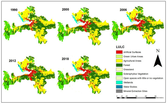
Figure 2.
LULC maps of the study area for 1990, 2000, 2006, 2012, and 2018.
The rise in the artificial surfaces is the most notable LULC development that has been observed between 1990 and 2018. The area of the city of İzmir was 19,418 ha in 1990 and 35,443 ha in 2018 (Table 5). A total of 11,721.25 ha of agricultural area, 1803.25 ha of forest, 1322.75 ha of grassland, and 492.5 hectares of sclerophyllous vegetation were transformed into artificial surfaces (Table 6). The period with the highest rate of change was between 1990 and 2000, when 8691.75 ha of agricultural land, 1483.50 ha forest, 954 ha of grassland, and 311.5 ha of sclerophyllous vegetation were converted into artificial surfaces. From 2000 to 2006, the rapid development process persisted. The majority of İzmir’s urban fabric was built on agricultural areas that sloped gently or almost flat on the urban periphery. Because of this, urban growth has had comparatively less of an impact on the forests and other natural areas in the highlands that surround these flat areas. A notable change here is the inclusion of approximately 94.25 ha of wetlands (83.5 ha of artificial surfaces and 10.75 ha of green urban areas) into the urban area. A large portion of this change has occurred in the Gediz Delta, which is protected by the Ramsar Convention and is situated on İzmir’s northern development axis.
Table 5.
LULC changes between 1990 and 2018.
Table 6.
Cross-tabulation of landscape change from 1990 to 2018 (ha).
3.2. Results of Habitat Quality Assessment
In terms of LULC classes, artificial surfaces and mining areas are the classes with no habitat value in all years (Table 7). Forest, sclerophyllous vegetation, wetland, and water classes were determined as the classes with the highest habitat quality value. While the habitat quality value of the grassland class was above average, the agricultural areas and open spaces with little or no vegetation classes were determined as areas with average habitat value. Artificial, non-agricultural vegetated areas have a low habitat value.
Table 7.
Habitat quality values according to LULC classes.
In order to examine the change in habitat quality in the study area over the years, habitat quality was divided into five classes and mapped based on previous studies (Figure 3). In terms of spatial distribution, areas with low habitat value are concentrated around İzmir Bay due to the development of human activities on the coastal areas. Furthermore, the development pattern of the city of İzmir has resulted in the concentration of areas with a high habitat value in areas with a hilly topography due to the development in areas with flat and nearly flat slopes that were previously used for agriculture. These areas include parts of the Yamanlar and Dede Mountains in the north, Mount Nif in the east, and parts of the Urla–Çeşme–Karaburun Peninsula in the southwest. The Gediz Delta, just northwest of İzmir, is the only remaining coastal area of high habitat value near the city of İzmir. In the southwest, areas of high habitat value around Urla continue along the coast.
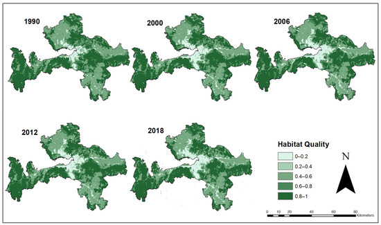
Figure 3.
Spatial distribution of habitat quality.
The changes between 1990 and 2000, 2006, 2012, and 2018 were calculated (Table 8). Although the areas with the highest habitat value tended to decrease between 1990 and 2018, it is seen that the habitat quality largely maintained its value. The most significant change in habitat quality occurred in areas with medium habitat quality. While the areas with medium habitat quality have decreased, the most important reason for the preservation of areas with high habitat quality is that the city of İzmir and its infrastructure are largely located on agricultural areas. It is seen that the artificial surfaces class, which has the lowest habitat quality, increased its distribution in the area from 5.69% to 10.65% between 1990 and 2018.
Table 8.
Habitat quality changes between 1990 and 2018.
The changes in the number and size of the patches with high habitat quality between 1990 and 2018 were also analyzed. Accordingly, the number of patches increased from 469 in 1990 to 606 in 2018 (Table 9). However, there was a decrease in the average patch size (from 394.31 ha to 297.39 ha) and the total area (from 184,932.21 ha to 180,221.28 ha) (Figure 4).
Table 9.
Features of the patches with the high habitat quality.
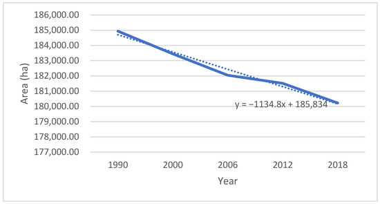
Figure 4.
Graph of Change in Total Area of High-Quality Habitat Patches with Trend Line.
3.3. Results of Habitat Importance for Connectivity
In this study, the delta versions of the IIC and PC indexes obtained with the Conefor 2.6 software were used to identify the nodes that are critical in terms of landscape connectivity within the patches with a high habitat quality. The delta version of the IIC (dIIC), which evaluates the connections between the habitat patches with a binary model, makes a simple assessment of whether or not there is a connection according to the size of the habitat patch, the distance between them, and the strength of the links between them, and expresses the importance of a patch as a percentage based on the change in landscape connectivity with the removal of the patch from the landscape. Based on a dIIC analysis of high-quality habitat patches between 1990 and 2018, there has been no significant change in the spatial pattern of important habitats in the immediate vicinity of İzmir (Figure 5). The calculation made with the delta version of the PC index, which calculates the connectivity between the patches with the probabilistic model by taking into account the probability of spread between two habitat patches, yielded a similar result (Figure 6). The dIIC and dPC results show that Mount Nif, in the east of the study area, and the Bozdağ foothills, which are partially located in the study area, constitute the most important habitats in terms of connectivity. The area located in the southwest of the study area, between the southern coast of the Urla district and the İzmir–Çeşme highway, is also critical for connectivity. The Mount Yamanlar foothills and associated patches in the north of the area are also among the most important patches in terms of connectivity.
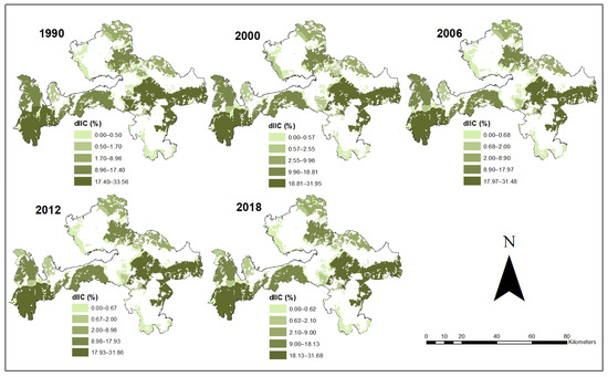
Figure 5.
Spatial distribution of the importance of habitats according to the dIIC index.
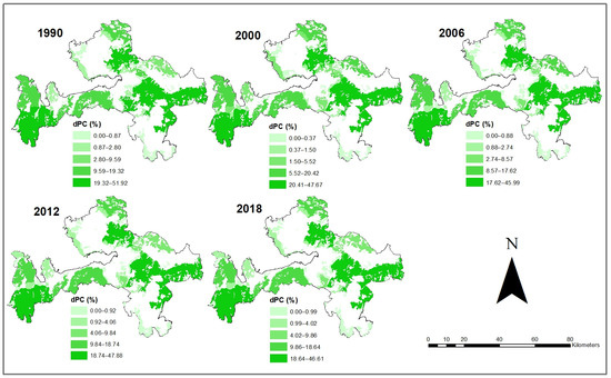
Figure 6.
Spatial distribution of the importance of habitats according to the dPC index.
When the dIIC and dPC values of all patches were evaluated for all study years, a threshold was observed in the patch importance for connectivity. Patches with values above this threshold remained consistently important across all years. Based on the ranking of the highest dIIC values in 1990, these 10 patches were identified as the key patches, and their dIIC and dPC values were separately analyzed over time (Table 10). However, patch 127 was excluded, since it could not be assessed as a whole patch in all the years. Accordingly, it was found that the dPC index, which evaluates the probability of connectivity between the patches, was generally higher than the dIIC. This pattern was consistent, except for patches 455 and 360, which exhibited a different trend. Moreover, although minor variations were observed in the patch importance rankings, the key patches identified by both indices remained the same. No significant changes in the patch importance were observed over the years.
Table 10.
The dIIC and dPC values of the most important patches for connectivity.
The area of change of the surveyed patches between 1990 and 2018 was also evaluated (Table 11). As explained earlier, there was no significant change in the size of the patches prioritized for connectivity, as the areas with a high habitat quality are some distance from the areas where human activities are concentrated. Only patch 385, where Mount Nif is located near Bornova and Kemalpaşa in İzmir, has seen a 19.03% decrease in size between 1990 and 2000. In addition, shrinkage was also observed in patches 387 and 391, which are located on the borders of the Urla district, and have been under the influence of second residences in the past and continuous settlement development in recent years. Patch 387 experienced a contraction of 7.78% between 1990 and 2000 and 3.73% between 2000 and 2006. Patch 391, on the other hand, experienced a steady decline between 1990 and 2018. As an important node between İzmir and the Urla–Çeşme–Karaburun Peninsula, which has largely preserved its natural structure, it is predicted that this loss will continue due to its proximity to the district center.
Table 11.
Changes over the years in the size of the most important patches for connectivity.
3.4. Results of the Evaluation of Changes in Possible Pathways Between Habitats
Important pathways for the connectivity of natural areas were generated using Circuitscape 4.0, based on the patch dPC values produced by Conefor 2.6. The analysis, which allowed for the generation of multiple pathway options, was conducted only for the years 1990 and 2018 to evaluate changes in the overall connectivity pattern (Figure 7). Although no significant change was observed in the spatial extent of high-quality habitats between 1990 and 2018 in earlier analyses, substantial changes were detected in potential important connectivity pathways due to the variation in the amount of resistance surface impeding corridor formation caused by LULC changes. In 1990, there was a notable density and number of potential connectivity pathways between the peninsula to the southwest of İzmir, Mount Nif and the Bozdağlar Mountains to the east, and Mount Yamanlar to the north, creating a belt-like structure around İzmir. However, by 2018, the formation of resistance surfaces resulting from the expansion of İzmir’s urban center had eliminated the likelihood of these corridors. In particular, it is understood that the possibility of connection with the peninsula region to the west of İzmir has largely disappeared.
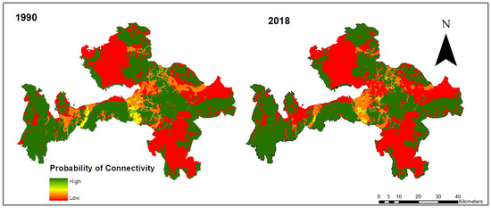
Figure 7.
Current maps generated in Circuitscape 4.0 showing connectivity in 1990 and 2018.
4. Discussion
This study evaluates how LULC changes between 1990 and 2018 have influenced habitat quality and landscape connectivity in İzmir. Despite significant urban expansion, areas of high habitat quality have largely remained intact, though increasing fragmentation poses challenges for maintaining ecological connectivity. The findings suggest that urbanization primarily replaced agricultural lands rather than directly impacting high-quality natural habitats. However, the emergence of resistance surfaces between the key habitat patches underscores the importance of integrating connectivity assessments into urban planning strategies.
Although the urban area of İzmir experienced significant development between 1990 and 2018, there was no significant change in the spatial pattern and the size of areas of high habitat quality. This result contradicts some studies that have demonstrated the negative effects of urban sprawl on habitat quality [6,7]. In addition, urban expansion has largely taken place on agricultural land. This was interpreted to mean that agricultural areas had negative impacts on habitat quality prior to intensive urbanization. This finding supports studies on the habitat quality of agricultural activities [8,9].
The topography of the İzmir metropolitan area significantly shapes LULC patterns. The city and its agricultural areas are situated between steep mountain ranges and coastal lowlands, forming natural barriers that constrain urban and agricultural expansion [141]. Consequently, urban growth follows an axial pattern along lowlands where agricultural activities are concentrated, while forested areas remain protected in higher elevations [142]. Additionally, rural-to-urban migration has led to a decline in agricultural and livestock activities, as many former farmers have shifted to alternative income sources, resulting in the abandonment of farmland and pastures [143,144]. This trend was further reinforced by Law No. 6360 (2012), which integrated rural settlements into metropolitan administration, altering land management and agricultural land use [145]. Between 1990 and 2018, forest areas expanded steadily, largely due to afforestation programs implemented by government institutions, NGOs, and private sector initiatives, contributing to the region’s increasing forest cover [146].
Despite the increase in artificial surfaces, areas of high habitat quality have remained largely intact. Although the number of high quality habitat patches increased between 1990 and 2018, their average size decreased. This can be interpreted as an indicator reflecting the fragmentation trend. It should be noted that there is a need for tools to assess the spatial structure of important habitats and corridors. In this context, evaluating the patches identified in this study with landscape metrics that allow the analysis and quantitative evaluation of spatial arrangements will provide a deeper perspective.
The relative importance of patches of a high habitat quality in terms of landscape connectivity was analyzed using Conefor 2.6 software. The critically important patches identified as a result of this analysis show similar results to previous studies conducted in İzmir. The parts of the important nature areas for Mount Nif, Alaçatı, the Bozdağlar Mountains, and Mount Yamanlar, which were identified as important nature areas for İzmir in Turkey’s Important Nature Areas Report, correspond to the first four patches identified as the most important in terms of connectivity [56]. The Gediz Delta important nature area, which is located on the northern development axis of the city of İzmir and has experienced significant urban development between 1990 and 2018, received low values in terms of both habitat quality and connectivity. Efforts to restore the wetland, which includes fresh, salt, and brackish water habitats and is home to 263 bird species, have gained momentum. However, in the analysis of possible connectivity corridors made with Circuitscape 4.0 software, it is understood that studies on the connectivity of the Gediz Delta with other habitats should be emphasized.
One of the interesting findings of this study is that, while no significant spatial change was observed between 1990 and 2018 in habitats with a high quality value and in habitat patches important in terms of connectivity in the study area, there was the development of significant resistance surfaces that could prevent the creation of corridors that would support connectivity between these areas. It is clear that landscape connectivity is an important parameter for supporting biodiversity and guaranteeing ecological functioning. Therefore, it is important to conduct detailed research and develop innovative approaches to alternative corridor design solutions.
The fact that the tools used in this study reveal İzmir’s important habitats and connectivity possibilities in a manner consistent with previous studies is encouraging for the evaluation of alternative future LULC change scenarios. In the literature, studies that have been conducted for this purpose are noteworthy. For example, Chen et al. (2023) examined the spatial and temporal evolution of habitat quality in the Yellow River Basin and multiple scenario predictions [15]. In addition, Sharma et al. (2018) simulated the impacts of LULC changes on biodiversity in Kalimantan, Indonesia, using the InVEST HQ model [92]. These studies are of great importance for identifying protected areas and restoration priorities.
In addition, as İzmir is located in the Mediterranean basin, which is expected to be most affected by climate change, there is a need to examine the long-term effects of climate change on habitat quality and connectivity. The inclusion of socio-economic data can increase an understanding of the drivers behind LULC changes and inform more holistic management approaches. The combined use of the InVEST HQ model, Conefor 2.6, and Circuitscape 4.0 in this study has demonstrated their usefulness in providing actionable insights for landscape management. However, future research could focus on refining these tools to account for species-specific behaviors and responses.
Limitations of Uncertainty and Future Recommended Works
While this study provides critical insights into LULC-driven habitat and connectivity changes, several limitations should be considered. First, although the findings align with previous studies on İzmir’s ecological structure, the absence of historical, species-specific movement data limits the validation of connectivity models. Future research should integrate empirical movement data to refine connectivity assessments.
Additionally, unlike many urbanizing regions where habitat loss is the dominant trend, this study indicates that, in İzmir, fragmentation and resistance surfaces are of greater concern. Comparing these findings with other Mediterranean and non-Mediterranean cities could provide a broader perspective on urbanization patterns and biodiversity impacts. Moreover, the results highlight the necessity of integrating connectivity analyses into urban planning. Policymakers should prioritize landscape-scale conservation strategies to mitigate fragmentation effects. Future research could explore scenario-based modeling approaches to assess the long-term effectiveness of alternative land management strategies.
Although the InVEST HQ model, Conefor 2.6, and Circuitscape 4.0 models are widely used in ecological and conservation studies, they inherently contain uncertainties due to model assumptions, input data quality, and methodological constraints. To address these issues, various validation techniques and sensitivity analyses have been implemented in prior research. Sensitivity analyses are commonly used to evaluate how variations in input parameters influence model outcomes, helping to manage uncertainty [92]. Additionally, integrating empirical field data and remote sensing techniques plays a crucial role in model calibration and validation, ensuring that predictions align with observed habitat conditions [147].
Despite these improvements, limitations persist. For instance:
- InVEST HQ assessments heavily depend on accurate LULC data and predefined threat parameters, which, if misclassified, can introduce uncertainty into the model outputs [84].
- Conefor 2.6’s effectiveness in landscape connectivity assessment relies on robust methodological frameworks, validation processes, and sensitivity analyses to refine model assumptions [148]. However, spatial resolution constraints in input data and the selection of dispersal parameters can introduce biases [149].
- Circuitscape 4.0’s resistance surface modeling provides a probabilistic representation of species movement across landscapes [150]. However, the model does not fully incorporate species-specific behavioral ecology, which may limit its capacity to accurately predict movement patterns [121]. Recent advancements, such as higher-resolution data processing capabilities, have improved Circuitscape 4.0’s efficiency and accuracy [151], but further refinements are still required.
This study also highlights the need for standardized classification indices in assessing habitat quality changes over time. Future research should focus on developing classification frameworks that enable comparative evaluations of habitat fragmentation trends across different regions. Furthermore, incorporating higher-resolution land cover datasets or remote sensing-based classifications could enhance the accuracy of future analyses.
Overall, advancements in ecological modeling and interdisciplinary approaches will be essential for reducing uncertainties and improving conservation planning applications. Integrating species-specific movement data, refining resistance values, and applying scenario-based modeling approaches will further enhance landscape connectivity assessments and contribute to sustainable urban planning strategies
5. Conclusions
This study assessed the impacts of LULC changes on habitat quality and landscape connectivity in İzmir between 1990 and 2018 using the InVEST HQ model, Conefor 2.6 connectivity analysis, and Circuitscape 4.0 resistance-based modeling. The findings indicate that urban expansion has significantly altered the spatial structure of natural habitats, leading to habitat fragmentation and an increased resistance to movement. Artificial surfaces increased by 82.5%, primarily replacing agricultural land, while the number of habitat patches rose from 469 in 1990 to 606 in 2018, highlighting intensified fragmentation. Connectivity analysis identified critical ecological corridors, particularly in Mount Nif and the Urla–Çeşme–Karaburun Peninsula, emphasizing their conservation importance. However, increased resistance values suggest a growing challenge for species movement and habitat connectivity.
These results underscore the necessity of integrating spatial modeling tools into urban and conservation planning to mitigate further habitat degradation. Policymakers and planners should prioritize ecological corridors and implement nature-based solutions to enhance connectivity in rapidly urbanizing landscapes. Future research should focus on refining model validation methods by incorporating long-term empirical datasets and assessing species-specific movement patterns to improve habitat quality and connectivity assessments. The findings contribute to broader biodiversity conservation strategies, reinforcing the need for sustainable land use policies that balance urban growth with ecological integrity.
Funding
This research received no external funding.
Institutional Review Board Statement
Ethical review or approval were not required for this study because it was non-interventional.
Informed Consent Statement
Not applicable.
Data Availability Statement
The data presented in this study are available upon request from the corresponding author.
Conflicts of Interest
The author declares no conflicts of interest.
References
- Yan, S.; Wang, X.; Cai, Y.; Li, C.; Yan, R.; Cui, G.; Yang, Z. An integrated investigation of spatiotemporal habitat quality dynamics and driving forces in the upper basin of Miyun reservoir, North China. Sustainability 2018, 10, 4625. [Google Scholar] [CrossRef]
- Zullo, F.; Montaldi, C.; Pietro, G.; Cattani, C. Land use changes and ecosystem services: The case study of the Abruzzo region coastal strip. ISPRS Int. J. Geo-Inf. 2022, 11, 588. [Google Scholar] [CrossRef]
- Meng, R.; Cai, J.; Hui, X.; Meng, Z.; Dang, X.; Han, Y. Spatio-temporal changes in land use and habitat quality of Hobq desert along the yellow river section. Int. J. Environ. Res. Public Health 2023, 20, 3599. [Google Scholar] [CrossRef] [PubMed]
- Ye, H.; Song, Y.; Xue, D. Multi-scenario simulation of land use and habitat quality in the Guanzhong plain urban agglomeration, China. Int. J. Environ. Res. Public Health 2022, 19, 8703. [Google Scholar] [CrossRef]
- Chun, F.; Liu, Y.; Chen, Y.; Li, F.; Huang, J.; Huang, H. Simulation of land use change and habitat quality in the yellow river basin under multiple scenarios. Water 2022, 14, 3767. [Google Scholar] [CrossRef]
- Chen, G.; Li, X.; Liu, X.; Chen, Y.; Liang, X.; Leng, J.; Xu, X.; Liao, W.; Qiu, Y.A.; Wu, Q.; et al. Global projections of future urban land expansion under shared socioeconomic pathways. Nat. Commun. 2020, 11, 537. [Google Scholar] [CrossRef]
- Li, G.; Fang, C.; Li, Y.; Wang, Z.; Sun, S.; He, S.; Qi, W.; Bao, C.; Ma, H.; Fan, Y.; et al. Global impacts of future urban expansion on terrestrial vertebrate diversity. Nat. Commun. 2022, 13, 1628. [Google Scholar] [CrossRef]
- Ding, Q.; Chen, Y.; Bu, L.; Ye, Y. Multi-scenario analysis of habitat quality in the Yellow River delta by coupling FLUS with InVEST model. Int. J. Environ. Res. Public Health 2021, 18, 2389. [Google Scholar] [CrossRef]
- Kija, H.K.; Ogutu, J.O.; Mangewa, L.J.; Bukombe, J.; Verones, F.; Graae, B.J.; Kideghesho, J.R.; Said, M.Y.; Nzunda, E.F. Spatio-temporal changes in wildlife habitat quality in the greater Serengeti ecosystem. Sustainability 2020, 12, 2440. [Google Scholar] [CrossRef]
- Ge, Y.; Li, C.; Zhang, T.; Wang, B. Temporal and spatial change of habitat quality and its driving forces: The case of Tacheng region, China. Front. Environ. Sci. 2023, 11, 1118179. [Google Scholar] [CrossRef]
- Zheng, H.; Li, H. Spatial–temporal evolution characteristics of land use and habitat quality in Shandong province, China. Sci. Rep. 2022, 12, 15422. [Google Scholar] [CrossRef] [PubMed]
- Hu, S.; Chen, L.; Li, L.; Zhang, T.; Yuan, L.; Cheng, L.; Wang, J.; Wen, M. Simulation of land use change and ecosystem service value dynamics under ecological constraints in Anhui province, China. Int. J. Environ. Res. Public Health 2020, 17, 4228. [Google Scholar] [CrossRef] [PubMed]
- Riva, F.; Nielsen, S. A functional perspective on the analysis of land use and land cover data in ecology. Ambio 2020, 50, 1089–1100. [Google Scholar] [CrossRef] [PubMed]
- Almeida, A.M.; Delgado, F.; Roque, N.; Ribeiro, M.; Fernandez, P. Multitemporal land use and cover analysis coupled with climatic change scenarios to protect the endangered taxon Asphodelus bento-rainhae subsp. bento-rainhae. Plants 2023, 12, 2914. [Google Scholar] [CrossRef]
- Chen, C.; Liu, J.; Bi, L. Spatial and temporal changes of habitat quality and its influential factors in China based on the InVEST model. Forests 2023, 14, 374. [Google Scholar] [CrossRef]
- Amininasab, S.; Kingma, S.; Birker, N.; Hildenbrandt, H.; Komdeur, J. The effect of ambient temperature, habitat quality and individual age on incubation behaviour and incubation feeding in a socially monogamous songbird. Behav. Ecol. Sociobiol. 2016, 70, 1591–1600. [Google Scholar] [CrossRef]
- Paraskevopoulou, Z.; Shamon, H.; Songer, M.; Ruxton, G.; McShea, W.J. Field surveys can improve predictions of habitat suitability for reintroductions: A swift fox case study. Oryx 2022, 56, 465–474. [Google Scholar] [CrossRef]
- Stoeckl, K.; Denic, M.; Geist, J. Conservation status of two endangered freshwater mussel species in Bavaria, Germany: Habitat quality, threats, and implications for conservation management. Aquat. Conserv. Mar. Freshw. Ecosyst. 2020, 30, 647–661. [Google Scholar] [CrossRef]
- Narce, M.; Meloni, R.; Beroud, T.; Pléney, A.; Ricci, J.C. Landscape ecology and wild rabbit (Oryctolagus cuniculus) habitat modeling in the Mediterranean region. Anim. Biodivers. Conserv. 2012, 35, 277–283. [Google Scholar] [CrossRef]
- Coates, P.S.; Casazza, M.L.; Ricca, M.A.; Brussee, B.E.; Blomberg, E.J.; Gustafson, K.B.; Overton, C.T.; Davis, D.M.; Niell, L.E.; Espinosa, S.P.; et al. Integrating spatially explicit indices of abundance and habitat quality: An applied example for greater sage-grouse management. J. Appl. Ecol. 2016, 53, 83–95. [Google Scholar] [CrossRef]
- Kahara, S.; Skalos, D.; Madurapperuma, B.; Hernandez, K. Habitat quality and drought effects on breeding mallard and other waterfowl populations in California, USA. J. Wildl. Manag. 2021, 86, e22133. [Google Scholar] [CrossRef]
- Sheehy, J.; Taylor, C.; Norris, D. The importance of stopover habitat for developing effective conservation strategies for migratory animals. J. Ornithol. 2011, 152, 161–168. [Google Scholar] [CrossRef]
- Zhang, Y.; Jiang, Z.; Li, Y.; Yang, Z.; Wang, X.; Li, X. Construction and optimization of an urban ecological security pattern based on habitat quality assessment and the minimum cumulative resistance model in Shenzhen city, China. Forests 2021, 12, 847. [Google Scholar] [CrossRef]
- Xing, X.; Liu, Y.; Jin, R.; Zhang, P.; Tong, S.; Zhu, W. Major role of natural wetland loss in the decline of wetland habitat quality—Spatio-temporal monitoring and predictive analysis. Sustainability 2023, 15, 12415. [Google Scholar] [CrossRef]
- Catry, I.; Franco, A.M.; Rocha, P.; Alcazar, R.; Reis, S.; Cordeiro, A.; Ventim, R.; Teodosio, J.; Moreira, F. Foraging habitat quality constrains effectiveness of artificial nest-site provisioning in reversing population declines in a colonial cavity nester. PLoS ONE 2013, 8, e58320. [Google Scholar] [CrossRef]
- Wu, L.; Sun, C.; Fan, F. Estimating the characteristic spatiotemporal variation in habitat quality using the invest model—A case study from Guangdong–Hong Kong–Macao Greater Bay Area. Remote Sens. 2021, 13, 1008. [Google Scholar] [CrossRef]
- Wang, B.; Cheng, W. Effects of land use/cover on regional habitat quality under different geomorphic types based on InVEST model. Remote Sens. 2022, 14, 1279. [Google Scholar] [CrossRef]
- Biggs, R.; Simons, H.; Bakkenes, M.; Scholes, R.J.; Eickhout, B.; van Vuuren, D.; Alkemade, R. Scenarios of biodiversity loss in southern Africa in the 21st century. Glob. Environ. Chang. 2008, 18, 296–309. [Google Scholar] [CrossRef]
- Leslie, T.; Griffiths, C. The Birds and Bees of Urban Biodiversity: Patterns, Problems, and a Path Forward. In The City is an Ecosystem; Routledge: London, UK, 2022; pp. 59–73. [Google Scholar]
- Jiang, D.; Zhang, Z.; Liu, B.; Zhang, X.; Zhang, W.; Chen, L. Spatiotemporal variations and driving factors of habitat quality in the loess hilly area of the yellow river basin: A case study of Lanzhou city, China. J. Arid Land 2022, 14, 637–652. [Google Scholar] [CrossRef]
- Tang, F.; Fu, M.; Wang, L.; Song, W.; Yu, J.; Wu, Y. Dynamic evolution and scenario simulation of habitat quality under the impact of land-use change in the Huaihe river economic belt, China. PLoS ONE 2021, 16, e0249566. [Google Scholar] [CrossRef]
- Liu, S.; Liao, Q.; Xiao, M.; Zhao, D.; Huang, C. Spatial and temporal variations of habitat quality and its response of landscape dynamic in the three gorges reservoir area, China. Int. J. Environ. Res. Public Health 2022, 19, 3594. [Google Scholar] [CrossRef]
- Imbrenda, V.; Lanfredi, M.; Coluzzi, R.; Simoniello, T. A smart procedure for assessing the health status of terrestrial habitats in protected areas: The case of the natura 2000 ecological network in Basilicata (southern Italy). Remote Sens. 2022, 14, 2699. [Google Scholar] [CrossRef]
- Wei, Y.; Wang, H.; Xue, M.; Yin, Y.; Qian, T.; Yu, F. Spatial and temporal evolution of land use and the response of habitat quality in Wusu, China. Int. J. Environ. Res. Public Health 2022, 20, 361. [Google Scholar] [CrossRef]
- Louis, V. Tiger habitat quality modelling in Malaysia with sentinel-2 and invest. Remote Sens. 2024, 16, 284. [Google Scholar] [CrossRef]
- Huo, A.; Liu, Q.; Zhao, Z.; Elbeltagi, A.; Abuarab, M.; Ganjidoust, H. Habitat quality assessment and driving factor analysis of xiangyu in feng river basin based on invest model. Water 2023, 15, 4046. [Google Scholar] [CrossRef]
- Chu, L.; Sun, T.; Wang, T.; Li, Z.; Cai, C. Evolution and prediction of landscape pattern and habitat quality based on CA-Markov and invest model in Hubei section of three gorges reservoir area (TGRA). Sustainability 2018, 10, 3854. [Google Scholar] [CrossRef]
- Aneseyee, A.; Noszczyk, T.; Soromessa, T.; Elias, E. The invest habitat quality model associated with land use/cover changes: A qualitative case study of the Winike watershed in the Omo-Gibe basin, southwest Ethiopia. Remote Sens. 2020, 12, 1103. [Google Scholar] [CrossRef]
- Luan, Y.; Huang, G.; Zheng, G.; Wang, Y. Correlation between spatio-temporal evolution of habitat quality and human activity intensity in typical mountain cities: A case study of Guiyang city, China. Int. J. Environ. Res. Public Health 2022, 19, 14294. [Google Scholar] [CrossRef]
- Luan, Y.; Huang, G.; Zheng, G. Spatiotemporal evolution and prediction of habitat quality in Hohhot city of China based on the invest and CA-Markov models. J. Arid Land 2023, 15, 20–33. [Google Scholar] [CrossRef]
- Terrado, M.; Sabater, S.; Chaplin-Kramer, B.; Mandle, L.; Ziv, G.; Acuña, V. Model development for the assessment of terrestrial and aquatic habitat quality in conservation planning. Sci. Total Environ. 2016, 540, 63–70. [Google Scholar] [CrossRef]
- Biswas, S.; Mallik, A.; Braithwaite, N.; Wagner, H. A conceptual framework for the spatial analysis of functional trait diversity. Oikos 2015, 125, 192–200. [Google Scholar] [CrossRef]
- Rowe, E.; Ford, A.; Smart, S.; Henrys, P.; Ashmore, M. Using qualitative and quantitative methods to choose a habitat quality metric for air pollution policy evaluation. PLoS ONE 2016, 11, e0161085. [Google Scholar] [CrossRef] [PubMed]
- Duarte, G.; Ribeiro, M.; Paglia, A. Ecosystem services modeling as a tool for defining priority areas for conservation. PLoS ONE 2016, 11, e0154573. [Google Scholar] [CrossRef] [PubMed]
- Hillman, J.; Lundquist, C.; Thrush, S. The challenges associated with connectivity in ecosystem processes. Front. Mar. Sci. 2018, 5, 364. [Google Scholar] [CrossRef]
- Fischer, J.; Lindenmayer, D.B. Landscape Modification and Habitat Fragmentation. Ecol. Manag. Restor. 2007, 8, 89–92. [Google Scholar] [CrossRef]
- Naiman, R.J.; Decamps, H.; Pollock, M. The Role of Riparian Corridors in Maintaining Biodiversity. BioScience 1993, 43, 209–218. [Google Scholar] [CrossRef]
- Pulsford, I.; Lindenmayer, D.; Wyborn, C.; Lausche, B.; Vasilijevic, M.; Worboys, G.L.; Lefroy, E. Connectivity Conservation Management; University of Tasmania: Hobart, Australia, 2015. [Google Scholar]
- Rosenberg, D.K.; Noon, B.R.; Meslow, E.C. Biological corridors: Form, function, and efficacy. BioScience 1997, 47, 677–687. [Google Scholar] [CrossRef]
- Magris, R.A.; Treml, E.A.; Pressey, R.L.; Weeks, R. Integrating multiple species connectivity and habitat quality into conservation planning for coral reefs. Ecography 2016, 39, 649–664. [Google Scholar] [CrossRef]
- Li, D.; Sun, W.; Xia, F.; Yang, Y.; Xie, Y. Can habitat quality index measured using the invest model explain variations in bird diversity in an urban area? Sustainability 2021, 13, 5747. [Google Scholar] [CrossRef]
- Baranyi, G.; Saura, S.; Podani, J.; Jordán, F. Contribution of habitat patches to network connectivity: Redundancy and uniqueness of topological indices. Ecol. Indic. 2011, 11, 1301–1310. [Google Scholar] [CrossRef]
- Salata, S.; Arslan, B. Designing with ecosystem modelling: The sponge district application in İzmir, Turkey. Sustainability 2022, 14, 3420. [Google Scholar] [CrossRef]
- Gülçin, D.; Yılmaz, T. Quantification of the Change in Ecological Connectivity Using a GIS-Based Model and Current Complexity Metrics. Int. J. Geogr. Geogr. Educ. 2020, 42, 689–701. [Google Scholar] [CrossRef]
- Bingöl, E. İzmir’de üretilen peyzajlar: JB Jackson’un peyzaj sınıfları üzerinden İzmir peyzajlarına yeniden bakış. Türkiye Peyzaj Araşt. Derg. 2020, 3, 40–56. [Google Scholar]
- Doğa Derneği. Türkiye’nin Önemli Doğa Alanları Cilt III; Eken, G., Bozdoğan, M., İsfendiyaroğlu, S., Kılıç, D.T., ve Lise, Y., Eds.; Doğa Derneği: Ankara, Türkiye, 2006; p. 80. [Google Scholar]
- IBB; EBRD. Izmir Green City Action Plan. Available online: https://ebrdgreencities.com/assets/Uploads/PDF/b5cbbe2fd1/Izmir-GCAP-report_FINAL-ISSUED-ENG-002.pdf (accessed on 30 December 2024).
- IBB; EBRD. Izmir Sustainable Energy and Climate Action Plan. Available online: https://mycovenant.eumayors.eu/storage/web/mc_covenant/documents/31/98KaWT7wBZ-ITIW1A7bpSrgh9rZmmGJ6.pdf (accessed on 30 December 2024).
- Velibeyoğlu, K.; Yazdani, H.; Baba, A. Groundwater in local development strategies: Case of Izmir. Water Sci. Technol. Water Supply 2018, 18, 1339–1349. [Google Scholar] [CrossRef]
- Sonmez, I.O. Re-emergence of suburbia: The case of Izmir Turkey. Eur. Plan. Stud. 2009, 17, 741–763. [Google Scholar] [CrossRef]
- Kandilli, C.; Ulgen, K. Solar illumination and estimating daylight availability of global solar irradiance. Energy Sources Part A 2008, 30, 1127–1140. [Google Scholar] [CrossRef]
- Isinkaralar, O.; Isinkaralar, K.; Yilmaz, D.; Öztürk, S. Multi-dimensional analysis of land use/land cover and urbanization on seasonal variation of land surface temperature in İzmir, Türkiye. Landsc. Ecol. Eng. 2025, 21, 133–150. [Google Scholar] [CrossRef]
- Lemenkova, P. Geospatial technology for land cover analysis. Middle East Afr. Geospat. Dig. 2013, 5. [Google Scholar] [CrossRef]
- Kesgin Atak, B.; Ersoy Tonyaloğlu, E. Monitoring the spatiotemporal changes in regional ecosystem health: A case study in Izmir, Turkey. Environ. Monit. Assess. 2020, 192, 385. [Google Scholar] [CrossRef]
- Coskun Hepcan, C. Quantifying landscape pattern and connectivity in a Mediterranean coastal settlement: The case of the Urla district, Turkey. Environ. Monit. Assess. 2013, 185, 143–155. [Google Scholar] [CrossRef]
- Öncel, H.; Levend, S. The effects of urban growth on natural areas: The three metropolitan areas in Türkiye. Environ. Monit. Assess. 2023, 195, 816. [Google Scholar] [CrossRef] [PubMed]
- Salata, S.; Erdoğan, B.; Ayruş, B. Designing Urban Green Infrastructures Using Open-Source Data—An Example in Çiğli, Izmir (Turkey). Urban Sci. 2022, 6, 42. [Google Scholar] [CrossRef]
- Baba, A.; Yazdani, H. Effect of Urbanization on Groundwater Resources of Izmir City. In Proceedings of the 4th International Water Congress, İzmir, Türkiye, 2–4 November 2017. [Google Scholar]
- Bossard, M.; Feranec, J.; Otahel, J. CORINE Land Cover Technical Guide—Addendum 2000; EEA Technical Report No 40; European Environment Agency: Copenhagen, Denmark, 2000.
- Feranec, J.; Hazeu, G.; Christensen, S.; Jaffrain, G. Corine land cover change detection in Europe (case studies of The Netherlands and Slovakia). Land Use Policy 2007, 24, 234–247. [Google Scholar] [CrossRef]
- Feranec, J.; Jaffrain, G.; Soukup, T.; Hazeu, G. Determining changes and flows in European landscapes 1990–2000 using CORINE land cover data. Appl. Geogr. 2010, 30, 19–35. [Google Scholar] [CrossRef]
- Ursu, A.; Stoleriu, C.C.; Ion, C.; Jitariu, V.; Enea, A. Romanian natura 2000 network: Evaluation of the threats and pressures through the Corine land cover dataset. Remote Sens. 2020, 12, 2075. [Google Scholar] [CrossRef]
- Giallonardo, T.; Landi, M.; Frignani, F.; Geri, F.; Lastrucci, L.; Angiolini, C. CORINE land cover and floristic variation in a Mediterranean wetland. Environ. Monit. Assess. 2011, 182, 141–154. [Google Scholar] [CrossRef]
- Zhu, M. Soil erosion risk assessment with CORINE model: Case study in the Danjiangkou reservoir region, China. Stoch. Environ. Res. Risk Assess. 2011, 26, 813–822. [Google Scholar] [CrossRef]
- Kandziora, M.; Burkhard, B.; Müller, F. Mapping provisioning ecosystem services at the local scale using data of varying spatial and temporal resolution. Ecosyst. Serv. 2013, 4, 47–59. [Google Scholar] [CrossRef]
- Muhacir, E.A.; Özalp, A.Y. Determining potential of coastal areas in producing ecosystem services by using AHP method: A case study in Artvin, Turkey. Asian J. Appl. Sci. 2015, 3, 779–788. [Google Scholar]
- Juknelienė, D.; Česonienė, L.; Jonikavičius, D.; Šileikienė, D.; Tiškutė-Memgaudienė, D.; Valčiukienė, J.; Mozgeris, G. Development of land cover naturalness in Lithuania on the edge of the 21st century: Trends and driving factors. Land 2022, 11, 339. [Google Scholar] [CrossRef]
- Olmedo, M.T.C.; García-Álvarez, D.; Gallardo, M.; Mas, J.F.; Paegelow, M.; Castillo-Santiago, M.Á.; Molinero-Parejo, R. Validation of Land Use Cover Maps: A Guideline. In Land Use Cover Datasets and Validation Tools; Springer: Cham, Switzerland, 2022; p. 35. [Google Scholar]
- Kale, Ö.A.; Baradan, S. Identifying factors that contribute to severity of construction injuries using logistic regression model. Tek. Dergi 2020, 31, 9919–9940. [Google Scholar] [CrossRef]
- Al-Bakri, J.T.; Duqqah, M.; Brewer, T. Application of remote sensing and GIS for modeling and assessment of land use/cover change in Amman/Jordan. J. Geogr. Inf. Syst. 2013, 5, 509–519. [Google Scholar] [CrossRef]
- Jiménez, A.A.; Vilchez, F.F.; González, O.N.; Flores, S.M.M. Analysis of the land use and cover changes in the metropolitan area of Tepic-Xalisco (1973–2015) through landsat images. Sustainability 2018, 10, 1860. [Google Scholar] [CrossRef]
- InVEST Habitat Quality Model User Guide. Available online: https://naturalcapitalproject.stanford.edu/invest/habitat-quality (accessed on 13 November 2024).
- Huang, H.; Xiao, Y.; Ding, G.; Liao, L.; Yan, C.; Liu, Q.; Gao, Y.; Xie, X. Comprehensive evaluation of island habitat quality based on the invest model and terrain diversity: A case study of Haitan island, China. Sustainability 2023, 15, 11293. [Google Scholar] [CrossRef]
- Li, F.; Wang, L.; Chen, Z.; Clarke, K.; Li, M.; Jiang, P. Extending the sleuth model to integrate habitat quality into urban growth simulation. J. Environ. Manag. 2018, 217, 486–498. [Google Scholar] [CrossRef]
- Sharp, R.; Tallis, H.T.; Ricketts, T.; Guerry, A.D.; Wood, S.A.; Chaplin-Kramer, R.; Nelson, E.; Ennaanay, D.; Wolny, S.; Olwero, N.; et al. InVEST 3.2.0 User’s Guide; The Natural Capital Project: Stanford, CA, USA, 2018. [Google Scholar]
- Chen, Y.; Qiao, F.; Jiang, L. Effects of land use pattern change on regional scale habitat quality based on InVEST model—A case study in Beijing. Acta Sci. Nat. Univ. Pekin. 2016, 52, 553–562. [Google Scholar]
- Tang, F.; Fu, M.; Wang, L.; Zhang, P. Land-use change in Changli County, China: Predicting its spatio-temporal evolution in habitat quality. Ecol. Indic. 2020, 117, 106719. [Google Scholar] [CrossRef]
- He, B.; Chang, J.; Guo, A.; Wang, Y.; Wang, Y.; Li, Z. Assessment of river basin habitat quality and its relationship with disturbance factors: A case study of the Tarim River Basin in Northwest China. J. Arid Land 2022, 14, 167–185. [Google Scholar] [CrossRef]
- Otgonbayar, M.; Tseveengerel, B.; Munkhtur, P.; Tuyagerel, D.; Chambers, J. Assessment of Habitat Quality in the Western Region of Mongolia Using the InVEST-Based Model. In Proceedings of the Environmental Science and Technology International Conference ESTIC 2021, Ulaanbaatar, Mongolia, 23 September 2021; Atlantis Press: Amsterdam, The Netherlands, 2021; pp. 96–101. [Google Scholar]
- Wei, P.; Chen, S.; Wu, M.; Deng, Y.; Xu, H.; Jia, Y.; Liu, F. Using the InVEST model to assess the impacts of climate and land use changes on water yield in the upstream regions of the Shule River Basin. Water 2021, 13, 1250. [Google Scholar] [CrossRef]
- Jeong, A.; Kim, M.; Lee, S. Analysis of Priority Conservation Areas Using Habitat Quality Models and MaxEnt Models. Animals 2024, 14, 1680. [Google Scholar] [CrossRef]
- Sharma, R.; Nehren, U.; Rahman, S.A.; Meyer, M.; Rimal, B.; Aria Seta, G.; Baral, H. Modeling land use and land cover changes and their effects on biodiversity in Central Kalimantan, Indonesia. Land 2018, 7, 57. [Google Scholar] [CrossRef]
- Sallustio, L.; De Toni, A.; Strollo, A.; Di Febbraro, M.; Gissi, E.; Casella, L.; Geneletti, D.; Munafò, M.; Vizzarri, M.; Marchetti, M. Assessing habitat quality in relation to the spatial distribution of protected areas in Italy. J. Environ. Manag. 2017, 201, 129–137. [Google Scholar] [CrossRef] [PubMed]
- Li, X.; Zhang, S.; Li, X.; Chen, R.; Huang, X.; Peng, J. Multi-scenario simulation and optimization of habitat quality under karst desertification management. Front. Environ. Sci. 2024, 12, 1495262. [Google Scholar] [CrossRef]
- Yang, J.; Xie, B.; Zhou, J. Research on the coupled evolution of LULCC and habitat quality in the Ganqing section of the Yellow River Basin based on multi-scenario simulations. Front. Ecol. Evol. 2024, 12, 1401291. [Google Scholar] [CrossRef]
- Abdollahi, S.; Zeilabi, E.; Xu, C.C. Habitat quality assessment based on local expert knowledge and landscape patterns for bird of prey species in Hamadan, Iran. Model. Earth Syst. Environ. 2024, 10, 2051–2061. [Google Scholar] [CrossRef]
- Wang, F.; McShea, W.J.; Wang, D.; Li, S.; Zhao, Q.; Wang, H.; Lu, Z. Evaluating landscape options for corridor restoration between giant panda reserves. PLoS ONE 2014, 9, e105086. [Google Scholar] [CrossRef]
- Carroll, C.; Fredrickson, R.; Lacy, R. Developing metapopulation connectivity criteria from genetic and habitat data to recover the endangered Mexican wolf. Conserv. Biol. 2013, 28, 76–86. [Google Scholar] [CrossRef]
- Barr, L.; Watson, J.; Possingham, H.; Iwamura, T.; Fuller, R. Progress in improving the protection of species and habitats in Australia. Biol. Conserv. 2016, 200, 184–191. [Google Scholar] [CrossRef]
- Tischendorf, L.; Fahrig, L. On the usage and measurement of landscape connectivity. Oikos 2000, 90, 7–19. [Google Scholar] [CrossRef]
- Theobald, D.M. Exploring the functional connectivity of landscapes using landscape networks. Ecology 2006, 87, 1873–1885. [Google Scholar]
- Jordán, F.; Baldi, A.; Orci, K.M.; Racz, I.; Varga, Z. Characterizing the importance of habitat patches and corridors in maintaining the landscape connectivity of a Pholidoptera transsylvanica (Orthoptera) metapopulation. Landsc. Ecol. 2003, 18, 83–92. [Google Scholar] [CrossRef]
- Pascual-Hortal, L.; Saura, S. Integrating landscape connectivity in broad-scale forest planning through a new graph-based habitat availability methodology: Application to capercaillie (Tetrao urogallus) in Catalonia (NE Spain). Eur. J. For. Res. 2008, 127, 23–31. [Google Scholar] [CrossRef]
- Urban, D.; Keitt, T. Landscape connectivity: A graph-theoretic perspective. Ecology 2001, 82, 1205–1218. [Google Scholar] [CrossRef]
- Bunn, A.G.; Urban, D.L.; Keitt, T.H. Landscape connectivity: A conservation application of graph theory. J. Environ. Manag. 2000, 59, 265–278. [Google Scholar] [CrossRef]
- Ricotta, C.; Stanisci, A.; Avena, G.C.; Blasi, C. Quantifying the network connectivity of landscape mosaics: A graph-theoretical approach. Community Ecol. 2000, 1, 89–94. [Google Scholar] [CrossRef]
- Pascual-Hortal, L.; Saura, S. Comparison and development of new graph-based landscape connectivity indices: Towards the priorization of habitat patches and corridors for conservation. Landsc. Ecol. 2006, 21, 959–967. [Google Scholar] [CrossRef]
- Saura, S.; Pascual-Hortal, L. A new habitat availability index to integrate connectivity in landscape conservation planning: Comparison with existing indices and application to a case study. Landsc. Urban Plan. 2007, 83, 91–103. [Google Scholar] [CrossRef]
- McGarigal, K.; Cushman, S.A.; Neel, M.C.; Ene, E. FRAGSTATS: Spatial Pattern Analysis Program for Categorical Maps; University of Massachusetts: Amherst, MA, USA, 2002. [Google Scholar]
- Mladenoff, D.J.; DeZonia, B. APACK 2.23 Analysis Software: User’s Guide; Forest Landscape Ecology Lab, Department of Forestry, UW-Madison: Madison, WI, USA, 2004. [Google Scholar]
- Saura, S.; Torné, J. Conefor Sensinode 2.2: A software package for quantifying the importance of habitat patches for landscape connectivity. Environ. Model. Softw. 2009, 24, 135–139. [Google Scholar] [CrossRef]
- García-Feced, C.; Saura, S.; Elena-Rosselló, R. Improving landscape connectivity in forest districts: A two-stage process for prioritizing agricultural patches for reforestation. For. Ecol. Manag. 2011, 261, 154–161. [Google Scholar] [CrossRef]
- Saura, S.; Vogt, P.; Velázquez, J.; Hernando, A.; Tejera, R. Key structural forest connectors can be identified by combining landscape spatial pattern and network analyses. For. Ecol. Manag. 2011, 262, 150–160. [Google Scholar] [CrossRef]
- Gil-Tena, A.; Brotons, L.; Fortin, M.J.; Burel, F.; Saura, S. Assessing the role of landscape connectivity in recent woodpecker range expansion in Mediterranean Europe: Forest management implications. Eur. J. For. Res. 2013, 132, 181–194. [Google Scholar] [CrossRef]
- Roy, A.; Bhattacharya, S.; Ramprakash, M.; Kumar, A.S. Modelling critical patches of connectivity for invasive Maling bamboo (Yushania maling) in Darjeeling Himalayas using graph theoretic approach. Ecol. Model. 2016, 329, 77–85. [Google Scholar] [CrossRef]
- Bodin, Ö.; Saura, S. Ranking individual habitat patches as connectivity providers: Integrating network analysis and patch removal experiments. Ecol. Model. 2010, 221, 2393–2405. [Google Scholar] [CrossRef]
- Saura, S.; Pascual-Hortal, L. Conefor Sensinode 2.2 User’s Manual: Software for Quantifying the Importance of Habitat Patches for Maintaining Landscape Connectivity Through Graphs and Habitat Availability Indices; University of Lleida: Lleida, Spain, 2007; Available online: www.conefor.org (accessed on 13 November 2024).
- Cabarga Varona, A.; Arroyo Hailvoto, N.L.; Nogués Linares, S. The function of plantation forestry in landscape connectivity. Appl. Ecol. Environ. Res. 2016, 14, 527–542. [Google Scholar] [CrossRef]
- Ramirez-Reyes, C.; Bateman, B.L.; Radeloff, V.C. Effects of habitat suitability and minimum patch size thresholds on the assessment of landscape connectivity for jaguars in the Sierra Gorda, Mexico. Biol. Conserv. 2016, 204, 296–305. [Google Scholar] [CrossRef]
- Niculae, M.I.; Nita, M.R.; Vanau, G.O.; Patroescu, M. Evaluating the functional connectivity of Natura 2000 forest patch for mammals in Romania. Procedia Environ. Sci. 2016, 32, 28–37. [Google Scholar] [CrossRef]
- D’Elia, J.; Brandt, J.; Burnett, L.J.; Haig, S.M.; Hollenbeck, J.; Kirkland, S.; Marcot, B.G.; Punzalan, A.; West, C.J.; Williams-Claussen, T.; et al. Applying circuit theory and landscape linkage maps to reintroduction planning for California condors. PLoS ONE 2019, 14, e0226491. [Google Scholar] [CrossRef]
- McRae, B.H. Isolation by resistance. Evolution 2006, 60, 1551–1561. [Google Scholar]
- McRae, B.H.; Dickson, B.G.; Keitt, T.H.; Shah, V.B. Using circuit theory to model connectivity in ecology, evolution, and conservation. Ecology 2008, 89, 2712–2724. [Google Scholar] [CrossRef]
- Brodie, J.F.; Giordano, A.J.; Dickson, B.; Hebblewhite, M.; Bernard, H.; Mohd-Azlan, J.; Anderson, J.; Ambu, L. Evaluating multispecies landscape connectivity in a threatened tropical mammal community. Conserv. Biol. 2015, 29, 122–132. [Google Scholar] [CrossRef]
- Dickson, B.G.; Roemer, G.W.; McRae, B.H.; Rundall, J.M. Models of regional habitat quality and connectivity for pumas (Puma concolor) in the southwestern United States. PLoS ONE 2013, 8, e81898. [Google Scholar] [CrossRef] [PubMed]
- Vasudev, D.; Fletcher, R.J. Incorporating movement behavior into conservation prioritization in fragmented landscapes: An example of western hoolock gibbons in Garo Hills, India. Biol. Conserv. 2015, 181, 124–132. [Google Scholar] [CrossRef]
- Bell, R.C.; Parra, J.L.; Tonione, M.; Hoskin, C.J.; Mackenzie, J.B.; Williams, S.E.; Moritz, C. Patterns of persistence and isolation indicate resilience to climate change in montane rainforest lizards. Mol. Ecol. 2010, 19, 2531–2544. [Google Scholar] [CrossRef] [PubMed]
- Yumnam, B.; Jhala, Y.V.; Qureshi, Q.; Maldonado, J.E.; Gopal, R.; Saini, S.; Srinivas, Y.; Fleischer, R.C. Prioritizing tiger conservation through landscape genetics and habitat linkages. PLoS ONE 2014, 9, e111207. [Google Scholar] [CrossRef]
- McClure, M.L.; Hansen, A.J.; Inman, R.M. Connecting models to movements: Testing connectivity model predictions against empirical migration and dispersal data. Landsc. Ecol. 2016, 31, 1419–1432. [Google Scholar] [CrossRef]
- Koen, E.L.; Bowman, J.; Sadowski, C.; Walpole, A.A. Landscape connectivity for wildlife: Development and validation of multispecies linkage maps. Methods Ecol. Evol. 2014, 5, 626–633. [Google Scholar] [CrossRef]
- Hodgson, J.A.; Thomas, C.D.; Dytham, C.; Travis, J.M.; Cornell, S.J. The speed of range shifts in fragmented landscapes. PLoS ONE 2012, 7, e47141. [Google Scholar] [CrossRef]
- Lawler, J.J.; Ruesch, A.S.; Olden, J.D.; McRae, B.H. Projected climate-driven faunal movement routes. Ecol. Lett. 2013, 16, 1014–1022. [Google Scholar] [CrossRef]
- Hall, K.R.; Anantharaman, R.; Landau, V.A.; Clark, M.; Dickson, B.G.; Jones, A.; Platt, J.; Edelman, A.; Shah, V.B. Circuitscape in Julia: Empowering dynamic approaches to connectivity assessment. Land 2021, 10, 301. [Google Scholar] [CrossRef]
- Schlacher, T.A.; Carracher, L.K.; Porch, N.; Connolly, R.M.; Olds, A.D.; Gilby, B.L.; Ekanayake, K.B.; Maslo, B.; Weston, M.A. The early shorebird will catch fewer invertebrates on trampled sandy beaches. PLoS ONE 2016, 11, e0161905. [Google Scholar] [CrossRef]
- Xie, Z.; Zhang, B.; Shi, Y.; Zhang, X.; Sun, Z. Changes and protections of urban habitat quality in Shanghai of China. Sci. Rep. 2023, 13, 10976. [Google Scholar] [CrossRef] [PubMed]
- Hamilton, C.M.; Martinuzzi, S.; Plantinga, A.J.; Radeloff, V.C.; Lewis, D.J.; Thogmartin, W.E.; Heglund, P.J.; Pidgeon, A.M. Current and future land use around a nationwide protected area network. PLoS ONE 2013, 8, e55737. [Google Scholar] [CrossRef] [PubMed]
- Gray, M.; Dickson, B.; Nussear, K.; Esque, T.; Chang, T. A range-wide model of contemporary, omnidirectional connectivity for the threatened Mojave desert tortoise. Ecosphere 2019, 10, e02847. [Google Scholar] [CrossRef]
- Leoncini, F.; Semenzato, P.; Febbraro, M.; Loy, A.; Ferrari, C. Come back to stay: Landscape connectivity analysis for the Eurasian otter (Lutra lutra) in the western Alps. Biodivers. Conserv. 2022, 32, 653–669. [Google Scholar] [CrossRef]
- Theobald, D.M.; Reed, S.E.; Fields, K.; Soule, M. Connecting natural landscapes using a landscape permeability model to prioritize conservation activities in the United States. Conserv. Lett. 2012, 5, 123–133. [Google Scholar] [CrossRef]
- Cushman, S.A.; McKelvey, K.S.; Hayden, J.; Schwartz, M.K. Gene flow in complex landscapes: Testing multiple hypotheses with causal modeling. Am. Nat. 2006, 168, 486–499. [Google Scholar] [CrossRef]
- Partigöç, N.S.; Aydın, C.; Tarhan, Ç. Çok kriterli karar verme yöntemi ve CBS kullanılarak yerleşime uygun alanların belirlenmesi: İzmir kenti örneği. Akad. Disiplinlerarası Bilimsel Araşt. Derg. 2017, 3, 55–70. [Google Scholar]
- İzmir Büyükşehir Belediyesi. 1/25,000 Ölçekli İzmir Büyükşehir Bütünü Çevre Düzeni Olanı Açıklama Raporu, İBŞB İmar ve Şehircilik Dairesi Başkanlığı Nazım Plan Şube Müdürlüğü. 2012, p. 269. Available online: www.izmir.bel.tr/YuklenenDosyalar/NazimImarPlani/3118480_13233.pdf (accessed on 13 November 2024).
- Yalçın, G.E.; Kara, F.Ö. Kırsal göç ve tarımsal üretime etkileri. Harran Tarım Ve Gıda Bilim. Derg. 2016, 20, 154–158. [Google Scholar] [CrossRef]
- Ahsan, M.M.; Duman, D. Kırsal yerleşimlerde gençlerin göç etme eğilimleri ve etkileri: Bitlis ili Adilcevaz ilçesi örneği. J. Acad. Value Stud. 2022, 8, 231–243. [Google Scholar]
- Ayyildiz, M.; Çiçek, A.; Ayyildiz, B. 6360 sayılı büyükşehir yasasının kırsal kesime olası etkileri. Nevşehir Bilim Ve Teknol. Derg. 2016, 5, 280–285. [Google Scholar] [CrossRef][Green Version]
- Erol, S.Y.; Göy, B. Sosyal sorumluluk amacıyla yapılan ağaçlandırma çalışmaları: Örnek olay incelemesi. Orman. Araştırma Derg. 2022, 9, 86–96. [Google Scholar] [CrossRef]
- Nolè, L.; Pilogallo, A.; Saganeiti, L.; Scorza, F.; Santos, L.; Murgante, B. Habitat degradation: A comparative study between Tomar (PT) and Potenza (IT). In Proceedings of the International Conference on Computational Science and Its Applications, Cagliari, Italy, 1–4 July 2020; Springer International Publishing: Cham, Switzerland, 2020; pp. 645–654. [Google Scholar]
- Torres, R.T.; Carvalho, J.; Serrano, E.; Helmer, W.; Acevedo, P.; Fonseca, C. Favourableness and connectivity of a Western Iberian landscape for the reintroduction of the iconic Iberian ibex Capra pyrenaica. Oryx 2017, 51, 709–717. [Google Scholar] [CrossRef]
- García-Antón, A.; Garza, V.; Traba, J. Connectivity in Spanish metapopulation of Dupont’s lark may be maintained by dispersal over medium-distance range and stepping stones. PeerJ 2021, 9, e11925. [Google Scholar] [CrossRef] [PubMed]
- Grafius, D.R.; Corstanje, R.; Siriwardena, G.M.; Plummer, K.E.; Harris, J.A. A bird’s eye view: Using circuit theory to study urban landscape connectivity for birds. Landsc. Ecol. 2017, 32, 1771–1787. [Google Scholar] [CrossRef] [PubMed]
- Anantharaman, R.; Hall, K.; Shah, V.; Edelman, A. Circuitscape in Julia: High performance connectivity modelling to support conservation decisions. arXiv 2019, arXiv:1906.03542. [Google Scholar]


Disclaimer/Publisher’s Note: The statements, opinions and data contained in all publications are solely those of the individual author(s) and contributor(s) and not of MDPI and/or the editor(s). MDPI and/or the editor(s) disclaim responsibility for any injury to people or property resulting from any ideas, methods, instructions or products referred to in the content. |
© 2025 by the author. Licensee MDPI, Basel, Switzerland. This article is an open access article distributed under the terms and conditions of the Creative Commons Attribution (CC BY) license (https://creativecommons.org/licenses/by/4.0/).