Abstract
In the oil and gas sectors, as well as in waste landfills, the commitment to greater sustainability is leading to increased efforts in the search for methane leaks, both to avoid the emission of a major greenhouse gas and to enable greater fuel recovery. For rapid leak detection and flow estimation, drone-mounted sensors are used, which require a balanced configuration of the detection and measurement system, adequate for the specific sensor used. In the present work, the search for methane leaks is carried out using a tunable diode laser absorption spectrometer (TDLAS) mounted on a drone. Once the survey is carried out, the data obtained feed the algorithms necessary for estimating the methane flow using the mass balance approach. Various algorithms are tested in the background measurement phases and in the actual detection phase, integrated with each other in order to constitute a single balanced set-up for the estimation of the flow emitted. The research methodology adopted is that of field testing through controlled releases of methane. Three different flows are released to simulate different emission intensities: 0.054, 1.91 and 95.9 kg/h. Various data configurations are developed in order to capture the set-up that best represents the emission situation. The results show that for the correction of methane background errors, the threshold that best fits appears to be the one that combines an initial application of the 2σ threshold on the mean values with the subsequent application of the new 2σ threshold calculated on the remaining values. Among the detection algorithms, however, the use of a threshold of the 75th percentile on a series of 25 consecutive readings to ascertain the presence of methane is reported as an optimal result. For a sustainable approach to become truly practicable, it is necessary to have effective and reliable measurement systems. In this context, the integrated use of the highlighted algorithms allows for a greater identification of false positives which are therefore excluded both from the physical search for the leak and from the flow estimation calculations, arriving at a more consistent quantification, especially in the presence of low-emission flows.
1. Introduction
Unmanned Aerial Systems (UASs), commonly referred to as drones, hold enormous potential to transform environmental monitoring. Equipped with advanced sensors, these systems present a unique opportunity to connect field-based observations with traditional aerial remote sensing. They deliver high-resolution spatial data across extensive areas while offering significant time and cost efficiency.
The widespread adoption of drone technology in recent years, combined with advancements in miniaturized sensors compatible with drones, has led to numerous applications in environmental monitoring [1], particularly in detecting and measuring methane emissions [2]. Methane, a potent greenhouse gas, has drawn increasing global attention due to its role in climate change. Efforts to reduce methane emissions have intensified, especially in sectors such as the oil and gas supply chain and waste landfills. As a result, many studies have focused on identifying and quantifying methane leaks.
In the context of waste landfills, drones have been deployed to identify fugitive biogas emissions. These applications range from locating emission sources [3,4,5,6] to measuring methane fluxes emitted from landfills [7,8]. Additionally, researchers have conducted controlled methane release experiments to refine and enhance flow quantification models [9] or to investigate specific parameters within such models [10,11,12]. Recent advancements are increasingly focused on integrating drone-based measurements with other monitoring approaches, such as ground-based methane sensors or infrared cameras, to achieve more comprehensive assessments [13,14,15,16].
The oil and gas industries, which manage substantial quantities of methane, must continuously tackle the challenges of emissions and atmospheric leakage. In order to increase the sustainability of these sectors, the EU Methane Strategy, with the associated regulation, has been enacted in the EU. The regulation introduces key rules aimed at enhancing the measurement, reporting, and verification of methane emissions in the energy sector. These measures are designed to pinpoint the precise locations and volumes of methane emissions, enabling a transition from estimations to direct measurements. This mandates the adoption of increasingly standardized measurement techniques, including site-level monitoring with sensors mounted on UASs. Therefore, over the past two years, various aspects of methane’s impact within this sector have been examined for monitoring using UAS technology [17,18,19,20]. For instance, the authors of [21] presented a measurement technique aimed at accurately quantifying greenhouse gas emissions. Another study [22] highlighted the use of airborne methods for inspecting natural gas pipelines. Meanwhile, study [23] examined source detection using a drone-based system with controlled methane releases, analyzing various detection algorithm parameters to balance false positive rates and detection probabilities.
In study [24], the authors compared various technologies used to quantify methane losses in natural gas midstream applications. They noted that drone-based measurements exhibit higher relative uncertainties compared to other systems. Therefore, we believe it is crucial to focus on improving these measurement systems to achieve more accurate and reliable results. This requires further research into detection technologies, correction algorithms, evaluation methods, and standardized usage protocols.
Whether the purpose is to search for a methane leak or to estimate the emitted flow, the various approaches are based on similar methodologies. Identifying a methane leak is a result of two fundamental steps: first, the methane present in the background is measured by carrying out a survey mainly in areas adjacent to the site of interest where there are no leaks. Once the background level is known, the survey is carried out in the areas exposed to methane leaks; the leak is identified as the measurement that exceeds the previously measured background. However, it is not at all simple to arrive at both an adequate measurement of the background and the recognition of an actual methane leak. This is influenced by several factors, including the type of sensor employed, the frequency of data acquisition, the meteorological and climatic conditions during the survey, the dispersion models applied, the flow estimation approaches, the algorithms used at various stages, and the data integration method adopted. The availability of more reliable measurement systems can, however, encourage the use of virtuous and innovative methods with a view to making production chains more sustainable. A more effective measurement system, in fact, would allow for easier identification of methane leaks and for reconstructing the emission framework of the context analyzed. This would encourage the adoption of remediation interventions with greater promptness, accelerating the ecological transition of the systems examined.
As regards the background, correcting measurement errors is among the first issues to be addressed after the field survey has been carried out. In practice, every field survey should begin with the measurement of the so-called background; as regards methane, it is known that it is present in the atmosphere at an average concentration of 2 ppm. However, on specific sites, it is possible to encounter air masses influenced by the presence of local or regional emissions which modify the background of that area [25].
The measurement of the instrument noise, i.e., the minimum measurement level that can actually be achieved by the sensor used, can also be included in the background measurement. In practice, the initial background measurement includes both issues of background atmospheric concentration and measuring instrument noise.
Every background measurement, during a survey aimed at researching fugitive methane emissions, is affected by these problems; therefore, all researchers have to tackle the data filtering operation as an essential activity of data analysis, through the development of specific algorithms.
The problem that has arisen is therefore the following: once a set of measurements has been carried out, how can the set of incorrect measurements be identified among them and therefore excluded from the analysis so that the background level is correctly identified?
Without this operation, points that are not emissive can be identified as emissive, with a consequent enormous waste of time in searching for them, or flow quantification errors of several orders of magnitude can occur [26].
However, for a detection algorithm to be truly usable, it must be able to balance false positives with actual emission points; the presence of a high number of false positives implies an excessive subsequent effort in searching for emissions that do not exist, with an enormous waste of time and high personnel costs. On the other hand, a very sensitive algorithm that eliminates many actual emission points in order to avoid the risk of incurring false positives is equally fallacious [27].
The second step, i.e., the recognition of a methane leak, must also be carried out with great care. In this case, the question that arises is the following: once the survey has been carried out, which measurements represent the actual presence of methane?
To answer both questions, error correction and detection algorithms must be developed specifically for the individual sensors used.
This study aims to establish a measurement set-up for quantifying methane flow during drone-based surveys. A positive aspect of the optimization of the methane flow measurement system through sensors on drones is the possibility of validating this method within the scope of site monitoring and control plans. The aim is to obtain emission inventories of the sites that are more representative of the real situation, also integrating the measurements performed with traditional flux chambers in the case of waste landfills. This is in order to achieve greater awareness among site managers that can translate into greater use of environmentally sustainable interventions directly in the field.
In our case, the sensor utilized is a tunable diode laser absorption spectrometer (TDLAS), a non-contact technology that operates in the near-infrared region. TDLAS determines the concentration of gasses such as water vapor, carbon dioxide, methane, and hydrogen sulfide by illuminating a gas sample at a specific wavelength. When exposed to electromagnetic radiation at a particular frequency, a molecule vibrates and absorbs energy. The wavelengths at which these absorptions occur are fixed, unique, and depend on the molecule’s structure and its molecular bonds [28]. In recent years, very compact sensors have been developed that use this technology and can be equipped on drones to perform useful measurements for environmental monitoring of sites. In particular, TDLAS sensors have been used in various case studies for monitoring methane emissions [29,30,31].
The present work aims to verify some correction algorithms applied to the background data of a survey campaign carried out via drone using a TDLAS methane sensor. Furthermore, various detection algorithms are to be tested to identify an actual methane leak.
The paper is structured as follows: it begins by describing the methodology, which involves conducting a series of field test campaigns. The equipment used and the rationale behind the surveys are then detailed. This is followed by a section presenting the results of the tests, which are subsequently discussed in the context of related studies from the literature. The paper concludes with the main findings and suggestions for future research.
2. Materials and Methods
The methodology employed involves field testing, with multiple drone-based survey campaigns conducted to gather experimental data under varying environmental conditions. The collected data are subsequently processed using a range of algorithms to verify their effectiveness in identifying and eliminating false positives (called “correction algorithms”) and in detecting the actual methane emission (called “detection algorithms”). The methane detection procedure is described in the flowchart presented in Figure 1. The main steps of the estimation of methane emission are summarized as follows:
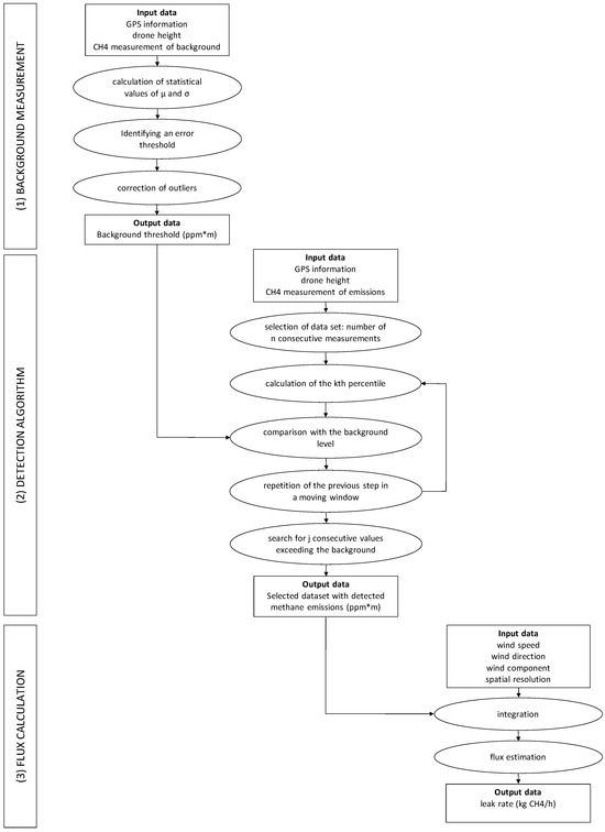
Figure 1.
A flowchart of the algorithm procedure.
- (1)
- Background estimation (application of the outlier correction algorithm);
- (2)
- Identification of emission points (application of the detection algorithm);
- (3)
- Calculation of the emitted methane flux (mass balance approach).
2.1. Methodology
2.1.1. Field Tests for Background Estimation: Correction Algorithms
The first step of these campaigns involves collecting data on the background methane levels measured by the instrument under different survey conditions. The collected data often includes inaccurate measurements, as some TDLAS sensors are prone to such issues, leading to the challenge of identifying outliers. In these instances, applying a correction algorithm can be helpful.
Once the outliers are eliminated, the background level is obtained; it will be used later as a threshold to identify the actual presence of methane. To this end, the following methods are adopted:
- (1)
- The individual observations ordered progressively according to the order of acquisition are divided into groups of 5 and the mean is calculated for each group. The original number of n observations is thus reduced to n/5 (which we will call “averaged observations” below). Among the averaged observations, always sorted progressively according to the order of acquisition/calculation, those that exceed a given threshold are highlighted as false positives.
Two simulations are performed with threshold values set at σ and 2σ above the mean. The standard deviation is calculated on the original values.
- (2)
- Another possibility is to apply the 2σ threshold directly to the original values and not to the averaged values.
- (3)
- We also attempt to intersect the 2σ threshold applied firstly to the averaged observations and then directly to the values.
- (4)
- A further method involves an iterative process in which the threshold of 2σ is updated every time values are eliminated, and the algorithm stops when skewness does not exceed the value of 0.5.
A study [29] suggested that skewness is a useful indicator for distinguishing between zero-leak and positive leak cases. Their tests showed that all zero-leak cases had skewness values below 0.5, while positive leak cases typically exhibited higher skewness values, above 0.5.
2.1.2. Field Tests with Controlled Methane Releases: Detection Algorithms
Once the right background level has been identified, these data are used as a threshold for identifying the actual presence of methane emissions. In this case, the tests carried out involve the controlled release of gas. Three different flows are released to simulate different emission intensities: 0.054, 1.91 and 95.90 kg/h. Also, in this case, various data configurations are developed in order to capture the set-up that best represents the emission situation (called “detection algorithms”). In practice, the distance from the potential emission point (soil/atmosphere interface) and the moving acquisition makes the exact correspondence between the position of the sensor (drone) and the possible anomaly on the ground more “blurry”. For this reason, it is necessary to “filter” and combine the numerous observations in order to highlight the sections of the drone’s path that show a significantly different signal compared to the neighboring sections.
The detection algorithm performs the following path:
- -
- It fixes a data set intended as a number n of consecutive measurements;
- -
- For each set of measurements, it takes a kth percentile as representative of the level of methane present in the sample;
- -
- The kth percentile is compared with the background level to identify the potential presence of methane;
- -
- It repeats the previous steps moving in a moving window of values;
- -
- Only in the presence of a minimum number j of consecutive values that have exceeded the background threshold, an actual emission of methane is considered in the original data set.
To make the algorithm work, the following values are tested:
n = 15, 25
k = 75th, 60th, 50th percentile
j = 5.
The different background levels obtained from the previous analysis are integrated into the detection algorithm to verify how the final emission results also vary as a function of this parameter.
2.1.3. The Methane Flux Estimation Model Used
The final result is expressed as the methane flux released, allowing for a comparison of the outcomes from applying different configurations of the described algorithm. This flux is calculated using the mass balance method, which has been frequently applied in recent years through measurements of atmospheric CH4 concentrations from aircraft or UAVs. This approach enables the estimation of surface gas exchanges, even in spatially heterogeneous conditions [32].
This method involves taking measurements downwind from the emission source so that the plume can be completely intercepted. It is then necessary to integrate these measurements into the vertical plane (x, z) through which the methane flows thanks to the movement caused by the wind in the component perpendicular to the plane. The CH4 flux is obtained through
where F indicates the emissive flux (g s−1), Ū⊥ is the component of wind speed (m s−1) perpendicular to the (x,z) plane, C is the measured concentration, Cb is the background concentration and x is the length of the trace while z is the height of the vertical plane with respect to the ground. The data are integrated both horizontally and vertically through specific interpolation algorithms [33].
In the present case, since a TDLAS sensor that already returns measurements indicating the methane column is used, integration on the vertical plane is not necessary.
Equation (1) is therefore simplified as follows:
where represents the concentration of CH4 integrated on the vertical plane.
2.1.4. An Alternative Method: Signal Detection, Processing and Feature Extraction
As reported, the defined method involves measuring the background with specific flights and subsequently subtracting it from the measurements made on the emitted plume. An alternative method can be provided by the signal detection method, already widely used in other fields, adapted to the estimation of methane. In general, signal detection is a process of interpretation of measured data that allows obtaining warning and diagnostic information. There are various examples of signal detection being used to perform electrostatic monitoring of multiple technologies [34], wear debris detection [35] and particle size measurement [36].
As previously mentioned, this exercise consists of highlighting the sections of the drone’s path that show a significantly different signal compared to the neighboring sections; in practice, it can be assimilated into a signal detection exercise.
Once the flight with the methane measurements has been carried out, the signal processing starts; it allows us to identify the main feature of the series of measurements. This feature is indicated as Activity Level (AL) and represents the characteristic amplitude of the recorded signal; in other words, in a series of data that mainly present a background noise, the Activity Level should represent a measurement close to the background noise. This is valid if the series of data is long enough to compensate for the presence of outliers and actual methane measurements.
Equation (3) reports the calculation of AL:
where AL(t) represents the signal amplitude at time t, in the presence of a total of N samples, and Cn represents the methane concentration of the nth sample [37].
It is assumed that methane is present if both of the following conditions occur:
- (1)
- The nth sample exceeds the value of AL or Cn > AL;
- (2)
- A number k of consecutive measurements satisfies condition (1).
Once the data are validated, the methane flux is measured using the mass balance method previously described.
Ultimately, with this method, the background value is obtained together with the validated emission values, by carrying out a single flight session and directly from the data of this flight.
In practice, however, this method is difficult to apply directly as illustrated, because in many cases, the series of data available is not sufficiently long and the presence of outliers as well as methane, both with high values, can result in an AL with a high value as well. In this circumstance, very few samples would pass condition (1) and consequently, it would be difficult to have a series k of consecutive measurements that satisfy condition (2). The result would be that it is not possible to identify the methane emission and therefore the detection fails in its task.
To overcome this problem, it is possible to pre-process the data using a filter as a smoothing method; [37] proposes the median filter in the case of noise removal in the electrostatic monitoring signal. In this work, various filters equal to the median, the 60th percentile and the 75th percentile of a series of measurements are tested. The filter acts as follows:
- (a)
- A step size s is defined for the data to be processed (in our case, s = 5 since the TDLAS sensor used returns a series of 5 measurements for each pair of recorded coordinates);
- (b)
- A sliding window of a specified length equal to a multiple x of the step size is defined (in our case, length = x s; x = 5);
- (c)
- The indicated filter is applied to the single window (median, 60th or 75th percentile);
- (d)
- The window is slid by the specified step size and step (c) is repeated until reaching the end of the data series.
In this way, the original data series is pre-processed and replaced by a data series represented, for example, by the median of each moving window, if the median was applied as a filter. These outputs are now used to feed Equation (3) and calculate the amplitude of AL; moreover, the two conditions described above are now applied for the detection of the series. The practical advantage of this approach is that a smoothed data series is obtained, which allows us to preliminarily eliminate the outliers and, moreover, it is not necessary to carry out separate flights for the background measurement.
2.2. Surveys Design and Locations
Background level measurements using a TDLAS sensor have been performed in various survey campaigns, which allows for the collection of experimental data in different ambient situations. Eighty flights were performed to test both flight variables and the surfaces flown over. This was to verify whether measurement errors are more prevalent in different environmental conditions. The effect of controllable and non-controllable variables on background measurement was reported in [38].
These surveys were carried out in Apulia (Italy) in situations that could simulate the surfaces of landfill or natural gas sites:
- -
- A suburban area (SA) with a surface covered with short grass;
- -
- A surface of a company in an industrial area (IA) consisting of gravel;
- -
- An agricultural field where cereals are grown (AA), with the presence of tall cereal plants.
During certain field trials, a controlled methane release test was conducted to assess whether varying background levels used in estimating methane emissions could produce differing results, depending on the specific conditions under which the measurements were taken.
The methane flux released in these tests was very low and equal to 0.054 kg/h.
Further controlled release tests were performed at two sites of natural gas infrastructure in Apulia and Emilia Romagna, Italy, to test higher fluxes in real situations. The releases were carried out with two vent stacks with heights of 3 m and 10 m, respectively. The methane content of the natural gas in the two cases was 94.3% and 93.9%, respectively, in standard conditions.
Table 1 reports the characteristics of the controlled release tests performed; it is clear what the logic followed in the design was. In practice, three types of emissions were tested:

Table 1.
Overview of methane release experiments.
- A very low one (0.054 kg/h), at the limit of the instrument’s ability to make the measurement, very close to the source and in particularly different environmental conditions;
- A medium one (1.91 kg/h), at a higher height, considered a challenging height for the instrument used;
- A super-emission (95.9 kg/h) far from the source.
The measurements were taken downwind of the emission source while the drone was flying perpendicular to the wind direction. The height and speed of the drone during the various surveys and the wind and ground conditions are reported in Table 1. The data acquisition frequency was configured at 10 Hz, ensuring high spatial resolution. During each survey, the flight followed the same straight path, traversing it back and forth multiple times to maximize the amount of collected information.
2.3. Instrumentation
The monitoring system used for data collection comprised various instruments.
2.3.1. Aerial Platform
The aerial platform is a rotary-wing drone, specifically a quadcopter, designed with technical and technological features to ensure precise surveys (Figure 2c). Its key features include the following:
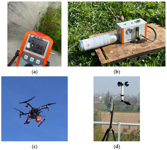
Figure 2.
Instrumentation used: (a) portable multi-function gas detector; (b) test set for controlled methane release (low rate); (c) drone equipped with TDLAS sensor; and (d) portable weather station.
- -
- An RTK system for enhanced positional accuracy;
- -
- Interconnection between the payload and the drone via SDK ports;
- -
- A multi-frequency radio control system for flight management;
- -
- An intelligent power system for reliable operation.
2.3.2. Payload
The UAV is equipped with a laser absorption spectrometer for methane detection using tunable diode laser absorption spectroscopy (TDLAS). The system operates by emitting laser light (wavelength: 1.65 μm) that reflects off the ground and is captured by the sensor. The outgoing and returning signals are compared against a built-in reference cell. Methane presence along the laser path partially absorbs the laser light, and an algorithm calculates the methane concentration in parts per million multiplied by the measurement path length (ppm*m). This sensor does not provide point measurements of methane at the drone’s altitude but instead measures the entire column of methane between the UAV and the ground.
The TDLAS sensor used was the Laser Falcon from Pergam, with the following main characteristics:
- -
- Sensing range: 1–50,000 ppm*m;
- -
- Detection accuracy: ±10%;
- -
- Response time: 0.1 s;
- -
- Detection distance: up to 30 m.
The laser operates at a data acquisition rate of 10 Hz. At a flight speed of 2 m/s, this configuration achieves a spatial resolution of 0.2 m.
TDLAS methane sensors are highly sensitive and capable of detecting methane at very low concentrations. Their tuning to specific absorption lines ensures high selectivity, enabling them to distinguish methane from other gasses. Studies, such as [39], have shown that these sensors are unaffected by laser intensity imperfections or spectral interference from other species and can accurately measure methane even in the presence of interfering compounds like benzene. This makes them suitable for identifying methane leaks in harsh environments and for environmental monitoring.
2.3.3. Portable Weather Station
During each test campaign, contextual environmental data were collected using an on-site portable weather station (Figure 2d). Parameters monitored included wind speed and direction, atmospheric pressure, humidity and air temperature.
2.3.4. Portable Multi-Function Gas Detector
To ensure accurate measurements, background methane levels in the area were first assessed to confirm that no methane was being emitted naturally. This was accomplished through an on-ground preliminary survey using a portable multi-function gas detector. The detector, equipped with selective sensors, can locate and classify gas-emitting points using a hybrid technology: a 0–1000 ppm semiconductor sensor for low concentrations and IR technology for higher concentrations (0.1–100% by volume). No methane emissions were detected during this survey (Figure 2a).
2.3.5. Controlled Methane Release Tests
For controlled methane release tests, a specialized test set was used, featuring the following:
- -
- A manometer (0–16 bar) to monitor test gas pressure;
- -
- An adjustable flowmeter (0–80 L/h);
- -
- Connections for various test gas cans (Figure 2b).
In controlled release tests conducted at the natural gas infrastructure with vent stack releases, the centralized control unit commanded the opening of the valves connected to the stacks and verified the outflow.
Figure 2 shows the instrumentation used for the analyses.
3. Results
3.1. Correction of Background Measurements
Several factors can influence the sensor’s ability to perform accurate measurements, leading to the presence of outliers in the data from each test. These outliers must be removed using specific correction algorithms. It is worth noting that some TDLAS sensors inherently exhibit this behavior, making outlier detection and correction a necessary step.
Figure 3 illustrates the measurements recorded during one of the flights conducted to assess background methane levels. This flight was carried out at a height of 10 m above ground level (AGL) and a drone speed of 1 m/s in a SA. The data shown in the figure represent the methane gas readings recorded by the sensor; as previously mentioned, the total amount of methane measured is expressed as the methane concentration (ppm) multiplied by the thickness (m), i.e., the methane column density (ppm*m). This type of sensor therefore measures the column of methane between the drone and the ground. For example, if methane is present in a measurement at a concentration of 100 ppm per 1 m of thickness, the sensor will return 100 ppm × 1 m = 100 ppm*m; in the same way, if in another measurement we find methane at a concentration of 200 ppm for a thickness of 0.5 m, the sensor will always return 200 ppm × 0.5 m = 100 ppm*m. Both measurements detect the same column density. All subsequent figures report the results in this same way.
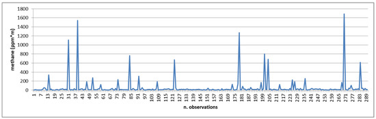
Figure 3.
Data collected during one of the flights conducted for background measurement at a height of 10 m AGL and a drone speed of 1 m/s, showing a significant number of outliers.
The figure highlights the presence of multiple methane peaks, some exceeding 1500 ppm*m, which are clear examples of sensor reading errors.
The primary cause of these false positive measurements lies in the scanning of non-homogeneous surfaces. As the detector moves along a horizontal path, variations in the reflectance of the target surface can disrupt the backscatter beam readings, particularly when amplified by sunlight. Additionally, sudden corrective movements of the drone, caused by strong winds or oscillations during flight, can produce similar errors.
For accurate analysis, these erroneous readings must be identified and excluded from the data set using correction algorithms. This ensures that only reliable measurements are considered in subsequent evaluations. In fact, considering such values in the calculations certainly leads to an error in estimating the correct background value. To this end, the procedures indicated in the previous section are applied to the data from the surveys carried out.
As an example, the results of a survey carried out in a SA and a second one carried out in an AA are reported, both at a drone speed of 1 ms−1. These surveys represent extreme situations with regard to the conditions in which the surveys were carried out. In fact, the first one was carried out in winter on a sunny day with an average wind speed of 2.2 ms−1, flying over an area covered with short vegetation. The second one was instead carried out flying over a wheat field with tall plants in the presence of a stronger wind, equal to 4.2 ms−1, which made the stems move.
The results of the application of the identified thresholds are shown in Table 2 and Table 3. The indicators reveal significant variability in the initial data, with notably high values for both the coefficient of variability and skewness. In this instance, despite the zero-leak condition, skewness values exceed 0.5 in the initial recordings, clearly indicating the presence of measurement errors.
Table 2.
Survey n. 1 in SA; flights at a speed of 1 ms−1; various altitudes. Statistical data of initial recorded measurement vs. results after the application of the correction algorithms.
Table 3.
Survey n. 1 in AA; flights at a speed of 1 ms−1; various altitudes. Statistical data of initial recorded measurement vs. results after the application of the correction algorithms.
The application of the indicated thresholds highlights a reduction in the values of both the mean and the standard deviation. However, from the comparison between methods, the method that is the most effective appears to be the one that combines an initial application of the 2σ threshold on the mean values with the subsequent application of the new 2σ threshold calculated on the remaining values (indicated in the tables as (3)). In fact, the first threshold allows the elimination of the highest peaks while the second, which is applied directly to the remaining detected values, eliminates the further anomalous values. Threshold (1a) also presents similar results to those of (3); in general, with this threshold, lower values than the mean and the final σ are obtained at the lowest heights (7 m and 10 m) but the skewness remains worse than the application of threshold (3). This trend is evident in both surveys shown here as an example but also in all the others not reported. Threshold (4) is the most likely to represent the real background situation since all the higher values have been eliminated until the remaining ones return a skewness lower than 0.5. This variability complicates the establishment of a lower threshold for background levels, as numerous false positives may be misinterpreted as actual methane leaks during subsequent leak detection efforts. Evidence of this problem will be provided in the subsequent analysis.
Figure 4 reports the remaining background values after applying algorithms (1a) and (3) to the data indicated in Figure 3. Ultimately, it turns out that the application of the first threshold does not filter some higher values that remain valid. The second threshold instead reduces the higher peaks; this behavior is more favorable, especially during the verification of the presence of methane, since the lower presence of peaks prevents these values from being identified as false positives.
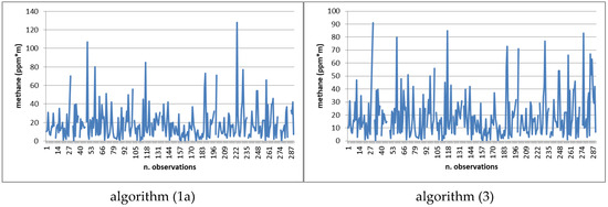
Figure 4.
Background measurements corrected with the application of algorithm (1a) and (3) (flight carried out at a height of 10 m AGL and at a drone speed of 1 ms−1).
3.2. Controlled Methane Release Tests Results Using Different Background Levels
As outlined in the Methodology Section, controlled methane release tests were conducted during some field trials to observe how data behave under varying background conditions. These tests also aimed to estimate methane flow while accounting for different background levels, where feasible.
Figure 5a,b present the results of these tests performed in a SA and AA, respectively. The two tests were conducted under markedly different conditions, as previously described. In Figure 5a, the methane peak is distinctly identifiable, following a predominantly Gaussian distribution with values that exceed the background level. Conversely, Figure 5b displays the raw data collected during methane release in AA, where multiple measurement peaks are observed. However, the characteristic pattern of methane emission is not discernible in this case.
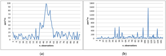
Figure 5.
Data collected during controlled methane release tests at a flight height of 7 m AGL and a drone speed of 1 m/s in SA (a) and AA (b) with respective wind speed of 2.2 and 4.2 m/s; methane release = 0.054 kg/h.
Figure 6 shows the data relating to air temperature and relative humidity recorded at 10 s intervals during survey no. 1 carried out in a SA. It can be noted that both environmental parameters have undergone very modest oscillations during the analyzed time interval: about 1 °C of temperature and about 4% of relative humidity. The comparison of these data with the gas measurements does not show any correlation that could generate an impact on the monitoring results. In fact, as indicated by [40], temperature is a very important environmental factor for most chemical sensors; the sensor temperature may fluctuate due to external temperature variations causing an unexpected signal. This issue affects most resistance-type sensors but particularly not the IR ones; in fact, only some IR absorption apparatuses have a temperature control function. Humidity is also a very important environmental factor, and the resistance and sensitivity of metal oxide semiconductor sensors can be affected by the adsorption of water molecules; as regards optical sensors, instead, if a wavelength of low absorption by water vapors is selected, it may theoretically be hardly affected by humidity.
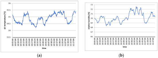
Figure 6.
Measurements of air temperature (a) and humidity (b) registered during the survey carried out in SA.
Table 4 shows the estimate of methane flow in all the controlled release tests; the different background levels are used in a methane flow estimation model based on the mass balance. For each test, the results of two tracks followed by the drone are presented; these results are expressed in percentage terms with respect to the actual release.
Table 4.
Estimation of methane flux versus actual release in all tests performed, using different background thresholds.
The different effects of the application of the various background thresholds can be noted depending on individual cases.
In general, it can be observed that the application of a lower threshold, (4), although more realistic, leads, in practice, to the validation of false positives in all cases. In the majority of tests, then, it produces an overestimation of the flow.
In the very-low-release tests, it can be observed that we are close to the detection limit of the system and that much depends on the ambient conditions observed at the time of the survey and on the threshold used. In fact, in test no. 2, using normal background thresholds, the leak is not detected and is confused with the background itself. By lowering the threshold, however, many areas are emissive, validating the outliers and leading to a very high estimation error. On the other hand, Figure 5b represents very well the situation in which the release blends perfectly with the environmental background and is indistinguishable from it.
In tests 1a and 1b, conducted in the same environmental conditions at different heights, the use of one threshold rather than another becomes decisive for the purpose of estimating the methane flux. In this case, with threshold (1b), the leak is very often not identified, while with the other thresholds, there is a strong variability in the estimates. Thresholds (1a) and (3) seem to present a similar performance, although they sometimes validate outliers.
In test no. 3, the higher flight height automatically implies a higher background; in this case, the variation in the background level obtained with the application of the various thresholds is modest in percentage terms (from a minimum of 207 ppm*m to a maximum of 270 ppm*m). The total estimate of the flow is therefore affected very little by the variation in the background and in fact, the results shown in the table are very stable.
Finally, in the presence of a super-emission of methane, the methane reading values are so high compared to the background that the variation in the background level becomes negligible compared to the estimate of the total flow.
In conclusion, when dealing with a low emission flow, the same methane release rate can either blend into the background or be detectable and measurable, depending on the background level used. However, this may also lead to the validation of false positives. This highlights the critical importance of understanding the optimal conditions for conducting measurements, particularly when attempting to detect low-flow leaks. Additionally, this underscores the significant impact that the chosen background threshold can have on the results.
In the presence of a very high flow or when flying at a higher altitude, the variation in the background level affects the estimation results less, although some thresholds still perform better than others.
3.3. Controlled Methane Release Test Results Using Different Detection Algorithms
As illustrated in the paragraph on methodology, the detection algorithm has the function of identifying, within a set of readings, which of them represents an actual methane emission. In essence, the algorithm considers the presence of a number j of consecutive readings that satisfy certain requirements as an emission; the requirements are related to the presence, within a moving window of a predetermined length (15 or 25 readings), of a value of a certain percentile (75th, 60th or 50th) that exceeds the background level. This exercise is conducted to verify which combination of parameters to choose that, within a certain number of values, presents a better performance in terms of estimating the flow. In addition to those indicated, further values were tested for the various parameters that led to unsatisfactory results; therefore, they were not reported in this study.
The results of this test, for all the controlled methane release tests, are presented in Table 5. The table reports the results of the six possible combinations of the two parameters (the third one is fixed). The results are expressed in terms of the percentage ratio between the estimate made with the application of a certain threshold and the actual flow. The background level chosen to perform the estimates is obtained with the application of threshold (3), defined previously.
Table 5.
Estimation of the methane flux compared to the actual release in all the tests carried out, using different detection algorithms.
The analysis of the results allows us to make several considerations:
- -
- The choice of the median (50th percentile) as a detection threshold, whether applied on 15 or 25 readings, is very restrictive in the case of low flows; it still allows us to identify the methane leak in other cases, although resulting in a generally underestimated flow; this choice can be considered precautionary and to be used especially if you want to be sure to intercept macro-leaks.
- -
- A smaller number of values on which to apply the chosen percentile, 15 instead of 25, represents a restricted sample of the track traveled; as a consequence, this leads to a greater estimation error both for excess and for defects and to the validation of a greater number of false positives.
- -
- In the presence of a macro-leak, each detection algorithm is able to identify such a leak even with an adequate order of magnitude of the estimate.
- -
- In the presence of a very low flow, the rapid dilution of the emitted methane in the air means that it can be identified by applying a less restrictive detection threshold, such as that represented by the 75th percentile.
- -
- In general, the detection algorithm that uses the 75th percentile as a threshold on 25 readings seems to have better effectiveness than the other combinations, also in terms of accuracy in the flow estimation.
- -
- The detection threshold of the 60th percentile on 25 readings has a performance similar to the previous one but with lower accuracy in the flow estimation; however, it does not report the validation of outliers. Therefore, it can be considered more conservative than the previous one but with a good level of effectiveness in the identification of the plume and in its estimation.
Of course, it must be considered that these results are referred and, therefore, are valid for a survey conducted with a high data acquisition frequency (10 Hz) with a drone flying at low speed (1–2 ms−1); the resulting high spatial resolution allows for mapping the emitted plume in greater detail.
3.4. Results Applying the Signal Detection Method
As highlighted in the Methodology Section, an alternative detection method is signal detection adapted to the methane survey with a drone. Figure 7 represents the contextual situation of test no. 4 performed on natural gas infrastructure. The flight path downwind of track no. 1 is highlighted with the interception of the methane plume represented by colored dots.
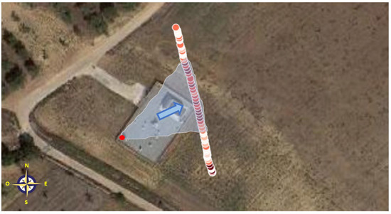
Figure 7.
Controlled methane release testing at natural gas infrastructure. Test n. 4. Track n. 1. Flight track and evidence of methane plume. The arrow indicates the direction of the wind; the colored dots highlight the presence of methane.
Figure 8a shows the original data recorded during the survey with the presence of some outliers. These data were pre-processed through the indicated filters leading to a smoothing of the curves represented in Figure 8b. The figure also reports the horizontal lines representing the respective Activity Levels calculated by applying the signal detection algorithm in the various cases. The methane identified as a leak is that which exceeds the Activity Level.
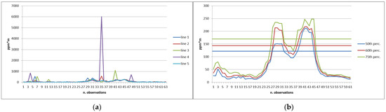
Figure 8.
Controlled methane release test n. 4., track n. 1. (a) Original values recorded along the route; each point corresponds to five measurements. (b) Smoothed values by applying the signal detection method with various detection thresholds and related Activity Levels.
A similar situation is also reported for test no. 1a for track no. 1 in Figure 9. This test is reported because it relates to a very reduced emission, unlike the previous one.
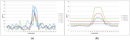
Figure 9.
Controlled methane release test n. 1a, track n. 1. (a) Original values recorded along the route; each point corresponds to five measurements. (b) Smoothed values by applying the signal detection method with various detection thresholds and related Activity Levels.
In both cases, it can be noted that the smoothed curves are cut by the AL not at the base of the peaks but at a certain height; in practice, a part of the plume is lost in the estimate.
Table 6 shows the results of this approach applied to the data obtained from all the controlled methane release tests. Also, in this case, the results are expressed as a percentage of the estimate compared to the actual flow.
Table 6.
Estimation of the methane flux with respect to the actual release in all the tests carried out, using the signal detection method with various smoothing filters.
First of all, it can be observed that with this approach, the emission is always identified, although in some cases there is also the validation of false positives. However, test no. 2 is an exception, in which the methane release is confused with the background, leading to a completely erroneous estimate.
Regarding the effectiveness of the estimate, as expected, the flow is generally underestimated. This happens because the AL obtained is generally high and, therefore, not perfectly representative of the background. In fact, the data series is not long enough to compensate for the effect of the actual methane measurements, and this leads to an AL higher than the background. This effect is partially reduced in test 1a compared to 4 because the section of the trace containing a different signal is lower percentage-wise. In fact, in test 1a, the section of the track containing the plume is equal to 2.5 m out of the 10 m total (25%), while in test 4, the section is 30 m out of 72 m (42%).
As for the filter used, there is no clear preference for one filter rather than another. In the reduced release tests, better results were obtained with the application of the 50th percentile to the data; in test 3 the 75th percentile performed better, while in test 4, the 60th percentile did.
4. Discussion
4.1. Background Measurement
In all the examined cases, the surveys carried out via drone to estimate the methane background in sites with no methane emissions produced a series of values that presented more or less large measurement errors. In particular, it is highlighted how statistical indicators can be useful in identifying the presence of errors. Various algorithms have been developed to correct the highlighted errors. With the presented algorithms, it is possible to correct sensor measurement errors.
The effectiveness of the correction, however, is variable and can be assessed by looking at the skewness indicator. It does not always fall below the value of 0.5 indicated by other authors in the literature, but in such cases, the value comes very close to it.
From the comparison between methods, the most effective method appears to be the one that combines an initial application of the 2σ threshold on the mean values with the subsequent application of the new 2σ threshold calculated on the remaining values, since it also balances the need not to correct the values too much for fear of not being able to avoid all false positives.
There are studies in the literature that have presented additional algorithms and different thresholds. Reference [10] corrected the local variation in measured background values using the robust extraction baseline signal (REBS) algorithm developed by [25]. This algorithm proposes an error correction procedure that applies a scale parameter σ obtained from the residuals below the mode. The threshold for the definition of zero-leak cases was indicated as the average of the background values +3σ. However, the same authors defined the estimation of the mode of an empirical distribution as a challenging exercise.
The study [41] indicated that the threshold of 2σ was optimal as most emissions are captured within this uncertainty threshold.
Another statistical method for estimating background values was proposed in the past by [42]. The method consisted of a procedure in various steps, in which a second-order polynomial fitted to minimum values recorded along a reference period was initially subtracted from the data. The parameter σ was obtained as the variability of the residual data that were smaller than the median of the residual distribution. The threshold of 3σ was indicated as representing a certainly emissive situation while the values between 2σ and 3σ were indicated as “possibly polluted”.
The threshold of 2σ has been indicated in the papers in which variability was calculated directly on the measured data without applying preliminary steps. The absolute value of σ in these cases can be high.
The threshold of 3σ has been indicated, however, in all the papers in which there was an initial step of subtraction of some minimum values from the measured data; in this case, the emission situation was characterized by a higher variability threshold since the absolute value of σ was lower than that calculated with the previous method whether it was applied to residuals below the mean, the median or the mode.
The procedure illustrated for identifying algorithms useful for solving the problem is easy to apply since it derives the values and thresholds directly from the measured data.
4.2. Detection Algorithms
With regard to detection algorithms, it can be observed that each researcher has tried to adapt a detection algorithm to the survey system used and to the data obtained.
Study [29] reported the use of skewness as a discriminant between zero-leak cases and releases as promising.
In study [31], the authors conducted a series of operations where the measured concentration was replaced with the cumulative concentration of all clearly identifiable peaks (defined by an overcoming of at least 50 ppm*m), rather than relying solely on the single highest point. This cumulative concentration was then divided by the total number of methane measurements.
However, ref. [25] reported that common detection methods based on a statistical approach rely on the identification of measurements that deviate from a smooth curve fit to the data. In this context, it becomes important to fix a series of adjacent or consecutive measurements that contain the emission signal. A critical issue that arises is how wide the local neighborhood should be. In our study, we directly and empirically tested some values and in the end identified the series of 15 and 25 values as valid, leaving out the others that had lower effectiveness in the estimate, in the case of high frequencies of data acquisition.
The results illustrated in the previous section show that among the various algorithms tested, the one that presents greater effectiveness in estimating the methane flow emitted is the application of a filter equal to the 75th percentile on a consecutive series of 25 readings, which exceeds the previously estimated background. The signal detection method also presents good effectiveness, especially in detecting the presence of a leak; in fact, it manages to identify the signal in all the cases examined, in a generalized way (test no. 2 is however problematic for all the methods). The estimate is less precise than the previous algorithm if a very long series of data is not available. And this can represent a problem in field applications since it would force the flight trajectories to be extended beyond the boundaries of the areas to be inspected to acquire a longer series of data containing a greater number of background measurements.
Ultimately, the choice of an appropriate detection algorithm represents a fundamental step in order to estimate the methane emission using measurements obtained from sensors mounted on drones.
4.3. Environmental Conditions Affecting Measurements
However, it should not be forgotten that in order to proceed with an estimate of the methane flow, the survey must be carried out in favorable environmental conditions. This is because it is always preferable to obtain a sensor response that contains a lower level of background and a smaller number of outliers before proceeding to apply the indicated algorithms.
In this regard, as noted in [38], the results from various field trials can identify the optimal conditions for measuring methane emissions with a TDLAS sensor to minimize the occurrence of outliers. These conditions include a flight altitude not exceeding 15 m AGL, with drone speed having a smaller impact on the results—though speeds between 1 and 2 m/s are ideal. Additionally, a sunny day results in much higher methane background levels compared to a cloudy day. The type of surface also plays a significant role in measuring background noise.
As regards wind intensity, wind can cause different stresses to the drone during flight, determining a different level of oscillation which in turn affects the oscillation of the beam transmitted by the laser; even the cover on the ground can move in the presence of wind (think, for example, of tall grasses) and this can affect the return reading to the sensor.
The illustrated tests, in fact, showed that it was possible to estimate methane flow, even with a very low emission rate, when flying over low-vegetation surfaces under favorable environmental conditions, which determined a low level of methane background. In the second test, the presence of an intense wind with associated gusts, on a surface characterized by tall plants, determined a high average concentration of methane background within which the actual gas release measurements were confused. Under these conditions, it was difficult to estimate the flow of gas released and it was easier to achieve false positives.
4.4. Spatial Resolution Affecting the Reconstruction of the Plume
As for the detection algorithms, we agree with what is indicated in study [30], which stated that the primary challenge in reconstructing gas plumes from integral measurements lies in developing algorithms that can effectively handle the highly dynamic nature of gas dispersion, as well as the sparsity of measurements. Therefore, the first relevant issue to consider is the spatial resolution obtained in the reconstruction of the plume. A low spatial resolution can allow the identification of macro-leaks while missing the smallest leaks. Since this factor depends on the flight speed and the acquisition frequency of the sensor, each survey must be planned according to these elements and the purpose of the detection. For example, [43] used a sampling rate of 1 Hz and a flight speed of 15–16 ms−1, which resulted in a low resolution of the methane. Reference [44] used a 10 Hz sampling rate combined with a speed of 12–18 ms−1, which gave a spatial resolution of 1.2–1.8 m.
For this reason, we decided to carry out the controlled release tests with a frequency of 10 Hz, flying at a low speed of 1–2 ms−1, in order to obtain a high spatial resolution (0.1–0.2 m). This allowed us to identify even smaller leaks such as those tested in survey no. 1.
By reprocessing the data obtained in the various tests and extracting the values at constant intervals, it was possible to simulate a lower spatial resolution (test no. 2 was omitted). In this case, however, it was necessary to reduce the numerical series in which to search for the emission values; we went from fifteen or twenty-five values (resolution 0.1–0.2 m), equal to a segment on the drone track of 1.5–5 m, to five or seven values (resolution 1–2 m), equal to a segment on the track of 5–14 m. On longer sections of the tracks, it would become more difficult to detect the differences in measurement and therefore the emission signal.
The results of this exercise are reported in Table 7. It can be noted that in tests with lower releases, sometimes even with a resolution of 1 m, it was not possible to identify the plume; however, with a resolution of 2 m, the emitted methane was not detected in any of these tests. In test 3, starting from a spatial resolution of 5 m, it was no longer possible to detect the emission. In the case of a macro-leak, however, at this resolution, the plume was identified, while for higher resolutions the data were not sufficient to carry out the simulation. In any case, the probability that some false positives could be mistaken for actual emissions increased, as can be seen from the table that reports more estimates that contain outliers than those illustrated previously.
Table 7.
Estimation of the methane flux compared to the actual release in the various tests carried out, simulating a different spatial resolution.
It can therefore be deduced that if, for example, a survey is carried out with a fixed-wing drone at a speed of 15 ms−1 and a sampling frequency of 2 Hz (spatial resolution 7.5 m), many emissions, even of non-negligible ranges, are missed. It then becomes essential to plan the mission according to objectives (e.g., identifying macro-leaks) and the available instrumentation (drone-sensor system).
4.5. Implications for Landfills and the Oil and Gas Sector
UAS methane detection may represent the new frontier in environmental monitoring; it will play a substantial role in identifying methane sources and enabling targeted mitigation, significantly reducing environmental impacts. With ongoing innovation, drones and sensors could revolutionize methane monitoring, becoming essential tools in combating climate change and promoting sustainability.
In order for this to happen, however, various international research groups are intensifying their efforts to provide reliable and repeatable methods. The greatest challenge is then to integrate these methods on a larger scale to assess the actual impact of landfills or natural gas infrastructures, which are among the main methane emitters.
The results of this work fit fully into this context. First of all, our results highlight the importance of performing controlled methane release tests aimed at completely defining the parameters involved in the methods identified. This observation is also shared by [45], who applied a different remote sensing technique aimed at researching and quantifying methane leaks. Reference [46] also proceeded with the validation of a drone-based method for quantifying fugitive methane emissions through controlled release tests, comparing the same measurements made with drones with simultaneous measurements obtained using the tracer gas dispersion method. Study [47] instead implemented a method for horizontal and vertical profiling of emission plumes capable of detecting leaks in the range of 0.04–1500 kg/h.
Secondly, the results of this work highlight that field measurement and subsequent data processing constitute a single integrated process aimed at finding a set-up that allows for increasing the effectiveness of estimates. This consideration becomes crucial, especially when considering the application of these methods in waste landfills. As [14] pointed out, the availability of reliable measurements referring to the landfill surface can facilitate remediation or repair interventions of the gas collection system by landfill managers. Study [48] also pointed out that an accurate quantification of methane emissions from landfills becomes crucial in mitigating the negative effects of climate change. The authors also recognize that traditional methods have significant limitations such as the presence of high uncertainties, in the case of estimates made by applying theoretical methane production models, or high operating costs, if one considers labor-intensive methods such as the use of land-boxes. Reference [49] reiterated the importance of measurement in the case of methane emissions from landfills compared to the application of models. In this work, in fact, the authors detected methane emissions from five Icelandic landfills, comparing the results of the data measured using tracer gas dispersion with those modeled through the IPCC FOD model; they concluded that the modeled emissions are overestimated compared to those measured in three out of five cases; the cause is probably to be found in the greater uncertainties present in the input data of the parameters used in the models.
In our work, we made an attempt to define a fine-tuning of the measurement system, especially to recognize small methane leaks. The detection of such leaks assumes considerable importance for both the oil and gas extraction and landfill sectors. For the oil and gas sector, study [50] reported that in the US many facilities emitting methane at low emission rates are often not detected. For 2021, the authors estimated that sites emitting at lower rates from smaller diffuse methane sources contribute overall to the majority of total emissions from oil and gas extraction sites.
A similar problem affects the landfill sector. In a study regarding the efficiency of Danish landfill collection systems, the authors reported that the real efficiency of such systems is often not assessed and that on average it is around 50% in reference to the analyzed landfills [51]. In another work, while measuring the emissions of two landfills in Michigan through various techniques, the authors identified both the active surfaces of the landfill and the collection system as the main sources of emissions [7]. In this regard, [52] identified a gap in the international literature referring to the comprehensive study of fugitive methane emissions from biogas collection systems while on the contrary there are guidelines relating to the assessment of the diffusion of biogas from landfill surfaces. Such studies are also essential in order to improve the assessment of the odorous impact of biogas emissions.
The problems highlighted are largely attributable to the identification and estimation of small methane emissions which, although they may be considered of little relevance if analyzed individually, overall can assume a considerable magnitude. In this context, the main findings of our work highlight the importance of defining methods that allow us to adequately process the collected raw data, especially to locate the high number of low-emitting point sources.
5. Conclusions
The reduction in methane emissions in the atmosphere is a challenging topic that is affecting many scholars around the world. In particular, this exercise requires that careful monitoring be carried out on sites where there may be fugitive emissions of gasses containing methane (such as in the oil and gas sector or in waste landfills). The technology of drones equipped with special sensors is proving to be very useful in carrying out site monitoring quickly and at low costs. However, the widespread diffusion of this technology requires the development of validated methods both for the identification of losses and for the estimation of emission flows.
One of the main problems that arise in the preparation of an estimation model is represented by the measurement of the background level and the noise of the instrumentation used. The present work illustrates the application of a series of error detection algorithms that allowed us to arrive at an adequate estimate of the background in measurements taken through a TDLAS sensor mounted on a drone. From the results, obtained through field trials, it is evident that it was possible to calculate reference thresholds to carry out a cut-off of incorrect measurements; the results were then compared with other correction procedures proposed in the literature.
Further tests were then performed that involved a controlled release of methane both with experimental equipment and on real sites of the natural gas infrastructure. These tests were aimed at verifying the effectiveness of a series of detection algorithms, modifying various parameters contained in them, such as the number of consecutive measurements to be considered, the filter representing the methane level in the sample and the number of consecutive measurements that exceeded the background threshold. The results showed the advantages and disadvantages of the application of the various algorithms and the level of effectiveness in estimating the methane flow emitted. Also, in this case, various data configurations were developed in order to capture the set-up that best represents the emission situation.
In conclusion, the results show that for the correction of methane background errors, in measurements carried out using a TDLAS sensor with a high data acquisition frequency, the threshold that best fits appears to be the one that combines an initial application of the 2σ threshold on the mean values with the subsequent application of the new 2σ threshold calculated on the remaining values. Among the detection algorithms, then, the use of a threshold of the 75th percentile on a series of 25 consecutive readings to ascertain the presence of methane is reported as an optimal result. The integrated use of the highlighted algorithms allows for a greater identification of false positives which are therefore excluded both from the physical search for the leak and from the flow estimation calculations, arriving at a more consistent quantification, especially in the presence of low emission flows.
Finally, the present work aimed to verify which set-up of the measurement system leads to a more effective estimate of the methane flux emitted. The tests performed included downwind flights to define a single track at a certain distance from the emission source. For future studies, it would be necessary to verify how the results can change in the presence of multiple tracks and multiple simultaneous emission sources.
Author Contributions
Conceptualization: G.T., L.C. and M.S.; methodology: G.T.; software, G.T.; validation: G.T., L.C. and M.S.; formal analysis, G.T.; investigation, G.T.; resources, G.T.; data curation, G.T.; writing—original draft preparation: G.T.; writing—review and editing, G.T., L.C. and M.S.; visualization, G.T., L.C. and M.S.; supervision, G.T.; project administration, G.T.; funding acquisition, G.T. All authors have read and agreed to the published version of the manuscript.
Funding
This article is part of the results of the research project “Integrated environmental monitoring via the use of Unmanned Aerial Systems (drones), environmental management systems and Life Cycle Assessment (LCA): set-up for improving the environmental profile of landfill sites and industrial plants”. PRIN—Progetti di Rilevante Interesse Nazionale 2022—Prot. 2022FPFPT5, settore ERC SH7—CUP H53D23004920006. Ministry of University and Research. Funded by European Union—Next Generation EU.
Institutional Review Board Statement
Not applicable.
Informed Consent Statement
Not applicable.
Data Availability Statement
The original contributions presented in this study are included in the article. Further inquiries can be directed to the corresponding author.
Conflicts of Interest
The authors declare no conflicts of interest.
References
- Manfreda, S.; McCabe, M.F.; Miller, P.E.; Lucas, R.; Pajuelo Madrigal, V.; Mallinis, G.; Ben Dor, E.; Helman, D.; Estes, L.; Ciraolo, G.; et al. On the Use of Unmanned Aerial Systems for Environmental Monitoring. Remote Sens. 2018, 10, 641. [Google Scholar] [CrossRef]
- Jonca, J.; Pawnuk, M.; Bezyk, Y.; Arsen, A.; Sówka, I. Drone-assisted monitoring of atmospheric pollution—A comprehensive review. Sustainability 2022, 14, 11516. [Google Scholar] [CrossRef]
- Soskind, M.G.; Li, N.P.; Moore, D.P.; Chen, Y.; Wendt, L.P.; McSpiritt, J.; Zondlo, M.A.; Wysocki, G. Stationary and drone-assisted methane plume localization with dispersion spectroscopy. Remote Sens. Environ. 2023, 289, 113513. [Google Scholar] [CrossRef]
- Daugela, I.; Visockiene, J.S.; Kumpiene, J. Detection and analysis of methane emissions from a landfill using unmanned aerial drone systems and semiconductor sensors. Detritus 2020, 10, 127–138. [Google Scholar] [CrossRef]
- Fjelsted, L.; Christensen, A.G.; Larsen, J.E.; Kjeldsen, P.; Scheutz, C. Assessment of a landfill methane emission screening method using an unmanned aerial vehicle mounted thermal infrared camera—A field study. Waste Manag. 2019, 87, 893–904. [Google Scholar] [CrossRef]
- Emran, B.J.; Tannant, D.D.; Najjaran, H. Low-Altitude Aerial Methane Concentration Mapping. Remote Sens. 2017, 9, 823. [Google Scholar] [CrossRef]
- Olaguer, E.P.; Jeltema, S.; Gauthier, T.; Jermalowicz, D.; Ostaszewski, A.; Batterman, S.; Xia, T.; Raneses, J.; Kovalchick, M.; Miller, S.; et al. Landfill Emissions of Methane Inferred from Unmanned Aerial Vehicle and Mobile Ground Measurements. Atmosphere 2022, 13, 983. [Google Scholar] [CrossRef]
- Allen, G.; Hollingsworth, P.; Kabbabe, K.; Pitt, J.R.; Mead, M.I.; Illingworth, S.; Roberts, G.; Bourn, M.; Shallcross, D.E.; Percival, C.J. The development and trial of an unmanned aerial system for the measurement of methane flux from landfill and greenhouse gas emission hotspots. Waste Manag. 2019, 87, 883–892. [Google Scholar] [CrossRef] [PubMed]
- Elpelt-Wessel, I.; Reiser, M.; Morrison, D.; Kranert, M. Emission Determination by Three Remote Sensing Methods in Two Release Trials. Atmosphere 2022, 13, 53. [Google Scholar] [CrossRef]
- Morales, R.; Ravelid, J.; Vinkovic, K.; Korbe, P.; Tuzson, B.; Emmenegger, L.; Chen, H.; Schmidt, M.; Humbel, S.; Brunner, D. Controlled-release experiment to investigate uncertainties in UAV-based emission quantification for methane point sources. Atmos. Meas. Tech. 2022, 15, 2177–2198. [Google Scholar] [CrossRef]
- Hollenbeck, D.; Zulevic, D.; Chen, Y.Q. Advanced leak detection and quantification of methane emissions using sUAS. Drones 2021, 5, 117. [Google Scholar] [CrossRef]
- Kim, Y.M.; Park, M.H.; Jeong, S.; Lee, K.H.; Kim, J.Y. Evaluation of error inducing factors in unmanned aerial vehicle mounted detector to measure fugitive methane from solid waste landfill. Waste Manag. 2021, 124, 368–376. [Google Scholar] [CrossRef] [PubMed]
- Liang, C.-W.; Zheng, Z.-C.; Chen, T.-N. Monitoring landfill volatile organic compounds emissions by an uncrewed aerial vehicle platform with infrared and visible-light cameras, remote monitoring, and sampling systems. J. Environ. Manag. 2024, 365, 121575. [Google Scholar] [CrossRef]
- Abichou, T.; Del’Angel, J.M.; Koloushani, M.; Stamatiou, K.; Belhadj Ali, N.; Green, R. Estimation of total landfill surface methane emissions using geospatial approach combined with measured surface ambient air methane concentrations. J. Air Waste Manage. Assoc. 2023, 73, 902–913. [Google Scholar] [CrossRef] [PubMed]
- Darynova, Z.; Blanco, B.; Juery, C.; Donnat, L.; Duclaux, O. Data assimilation method for quantifying controlled methane releases using a drone and ground-sensors. Atmos. Environ. X 2023, 17, 100210. [Google Scholar] [CrossRef]
- Abichou, T.; Bel Hadj Ali, N.; Amankwah, S.; Green, R.; Howarth, E.S. Using Ground- and Drone-Based Surface Emission Monitoring (SEM) Data to Locate and Infer Landfill Methane Emissions. Methane 2023, 2, 440–451. [Google Scholar] [CrossRef]
- Karam, S.N.; Bilal, K.; Shuja, J.; Rehman, F.; Yasmin, T.; Jamil, A. Inspection of unmanned aerial vehicles in oil and gas industry: Critical analysis of platforms, sensors, networking architecture, and path planning. J. Electron. Imaging 2023, 32, 011006. [Google Scholar] [CrossRef]
- de Smet, T.S.; Nikulin, A.; Balrup, N.; Graber, N. Successful Integration of UAV Aeromagnetic Mapping with Terrestrial Methane Emissions Surveys in Orphaned Well Remediation. Remote Sens. 2023, 15, 5004. [Google Scholar] [CrossRef]
- Smith, B.J.; Buckingham, S.; Touzel, D.F.; Corbett, A.M.; Tavner, C. Development of Methods for Top-Down Methane Emission Measurements of Oil and Gas Facilities in an Offshore Environment Using a Miniature Methane Spectrometer and Long-Endurance Uncrewed Aerial System. SPE Prod. Oper. 2024, 38, 565–577. [Google Scholar]
- Filkin, T.; Lipin, I.; Sliusar, N. Integrating a UAV System Based on Pixhawk with a Laser Methane Mini Detector to Study Methane Emissions. Drones 2023, 7, 625. [Google Scholar] [CrossRef]
- Corbett, A.; Smith, B. A Study of a Miniature TDLAS System Onboard Two Unmanned Aircraft to Independently Quantify Methane Emissions from Oil and Gas Production Assets and Other Industrial Emitters. Atmosphere 2022, 13, 804. [Google Scholar] [CrossRef]
- Iwaszenko, S.; Kalisz, P.; Słota, M.; Rudzki, A. Detection of Natural Gas Leakages Using a Laser-Based Methane Sensor and UAV. Remote Sens. 2021, 13, 510. [Google Scholar] [CrossRef]
- Tassielli, G.; Cananà, L. Environmental monitoring via drone: Development of algorithms for correcting background measurements. In Proceedings of the XXXII National Congress on Commodity Science, Lecce, Italy, 19–20 September 2024. [Google Scholar]
- Liu, Y.; Paris, J.-D.; Broquet, G.; Bescós Roy, V.; Meixus Fernandez, T.; Andersen, R.; Russu Berlanga, A.; Christensen, E.; Courtois, Y.; Dominok, S.; et al. Assessment of current methane emission quantification techniques for natural gas midstream applications. Atmos. Meas. Tech. 2024, 17, 1633–1649. [Google Scholar] [CrossRef]
- Ruckstuhl, A.F.; Henne, S.; Reimann, S.; Steinbacher, M.; Vollmer, M.K.; O’Doherty, S.; Buchmann, B.; Hueglin, C. Robust extraction of baseline signal of atmospheric trace species using local regression. Atmos. Meas. Tech. 2012, 5, 2613–2624. [Google Scholar] [CrossRef]
- Cambaliza, M.O.L.; Shepson, P.B.; Caulton, D.R.; Stirm, B.; Samarov, D.; Gurney, K.R.; Turnbull, J.; Davis, K.J.; Possolo, A.; Karion, A.; et al. Assessment of uncertainties of an aircraft-based mass balance approach for quantifying urban greenhouse gas emissions. Atmos. Chem. Phys. 2014, 14, 9029–9050. [Google Scholar] [CrossRef]
- Barchyn, T.E.; Hugenholtz, C.H.; Fox, T.A. Plume detection modeling of a drone-based natural gas leak detection system. Elem. Sci. Anth. 2019, 7, 41. [Google Scholar] [CrossRef]
- Stockwell, P. Tunable Diode Laser (TDL) Systems for Trace Gas Analysis. Meas. Control 2007, 40, 272–277. [Google Scholar] [CrossRef]
- Yang, S.; Talbot, R.W.; Frish, M.B.; Golston, L.M.; Aubut, N.F.; Zondlo, M.A.; Gretencord, C.; McSpiritt, J. Natural Gas Fugitive Leak Detection Using an Unmanned Aerial Vehicle: Measurement System Description and Mass Balance Approach. Atmosphere 2018, 9, 383. [Google Scholar] [CrossRef]
- Neumann, P.P.; Kohlhoff, H.; Hüllmann, D.; Krentel, D.; Kluge, M.; Dzierliński, M.; Lilienthal, A.J.; Bartholmai, M. Aerial-based gas tomography—From single beams to complex gas distributions. Eur. J. Remote Sens. 2019, 52 (Suppl. S3), 2–16. [Google Scholar] [CrossRef]
- Golston, L.M.; Aubut, N.F.; Frish, M.B.; Yang, S.; Talbot, R.W.; Gretencord, C.; McSpiritt, J.; Zondlo, M.A. Natural Gas Fugitive Leak Detection Using an Unmanned Aerial Vehicle: Localization and Quantification of Emission Rate. Atmosphere 2018, 9, 333. [Google Scholar] [CrossRef]
- Sliusar, N.; Filkin, T.; Huber-Humer, M.; Ritzkowski, M. Drone technology in municipal solid waste management and landfilling: A comprehensive review. Waste Manag. 2022, 139, 1–16. [Google Scholar] [CrossRef] [PubMed]
- Shaw, J.T.; Shah, A.; Yong, H.; Allen, G. Methods for quantifying methane emissions using unmanned aerial vehicles: A review. Phil. Trans. R. Soc. A 2021, 379, 20200450. [Google Scholar] [CrossRef]
- Wen, Z.; Hou, J.; Atkin, J. A review of electrostatic monitoring technology: The state of the art and future research directions. J. P. Aero. Sci. 2017, 94, 1–11. [Google Scholar] [CrossRef]
- Harvey, T.; Morris, S.; Wang, L.; Wood, R.; Powrie, H. Real-time monitoring of wear debris using electrostatic sensing techniques. Proc. Inst. Mech. Eng. Part J J. Eng. Tribol. 2007, 221, 27–40. [Google Scholar] [CrossRef]
- Tajdari, T.; Rahmat, M.F.; Wahab, N.A. New technique to measure particle size using electrostatic sensor. J. Electrost. 2014, 72, 120–128. [Google Scholar] [CrossRef]
- Wen, Z.; Zhao, X. A hybrid de-noising method based on wavelet and median filter for aero-engines gas path electrostatic monitoring. In Proceedings of the 2011 International Conference on Graphic and Image Processing, International Society for Optics and Photonics, Cairo, Egypt, 1–3 October 2011; p. 82852G-82852G-82857. [Google Scholar]
- Tassielli, G.; Cananà, L.; Spalatro, M. Detection of Methane Leaks via a Drone-Based System for Sustainable Landfills and Oil and Gas Facilities: Effect of Different Variables on the Background-Noise Measurement. Sustainability 2024, 16, 7748. [Google Scholar] [CrossRef]
- Mhanna, M.; Sy, M.; Farooq, A. A selective laser-based sensor for fugitive methane emissions. Sci. Rep. 2023, 13, 1573. [Google Scholar] [CrossRef] [PubMed]
- Noh, D.; Oh, E. Chemical Detection Using Mobile Platforms and AI-Based Data Processing Technologies. J. Sens. Actuator Netw. 2025, 14, 6. [Google Scholar] [CrossRef]
- Robertson, A.M.; Edie, R.; Snare, D.; Soltis, J.; Field, R.A.; Burkhart, M.D.; Bell, C.S.; Zimmerle, D.; Murphy, S.M. Variation in Methane Emission Rates from Well Pads in Four Oil and Gas Basins with Contrasting Production Volumes and Compositions. Environ. Sci. Technol. 2017, 51, 8832–8840. [Google Scholar] [CrossRef]
- O’Doherty, S.; Simmonds, P.; Cunnold, D.; Wang, H.; Sturrock, G.; Fraser, P.; Ryall, D.; Derwent, R.; Weiss, R.; Salameh, P.; et al. In situ chloroform measurements at Advanced Global Atmospheric Gases Experiment atmospheric research stations from 1994 to 1998. J. Geophys. Res. 2001, 106, 20429–20444. [Google Scholar] [CrossRef]
- Barchyn, T.E.; Hugenholtz, C.H.; Myshak, S.; Bauer, J. A Uav-based system for detecting natural gas leaks. J. Unmanned Veh. Sys. 2017, 6, 18–30. [Google Scholar] [CrossRef]
- Hollenbeck, D.; Dahabra, M.; Christensen, L.E.; Chen, Y.Q. Data quality aware flight mission design for fugitive methane sniffing using fixed wind sUAS. In Proceedings of the 2019 International Conference on Unmanned Aircraft Systems (ICUAS), Atlanta, GA, USA, 11–14 June 2019. [Google Scholar]
- Foster-Wittig, T.A.; Thoma, E.D.; Albertson, J.D. Estimation of point source fugitive emission rates from a single sensor time series: A conditionally-sampled Gaussian plume reconstruction. Atmos. Environ. 2015, 115, 101–109. [Google Scholar] [CrossRef]
- Scheutz, C.; Knudsen, J.E.; Vechi, N.T.; Knudsen, J. Validation and demonstration of a drone-based method for quantifying fugitive methane emissions. J. Environ. Manag. 2025, 373, 123467. [Google Scholar] [CrossRef] [PubMed]
- Dooley, J.F.; Minschwaner, K.; Dubey, M.K.; El Abbadi, S.H.; Sherwin, E.D.; Meyer, A.G.; Follansbee, E.; Lee, J.E. A new aerial approach for quantifying and attributing methane emissions: Implementation and validation. Atmos. Meas. Tech. 2024, 17, 5091–5111. [Google Scholar] [CrossRef]
- Yong, H.; Allen, G.; Mcquilkin, J.; Ricketts, H.; Shaw, J.T. Lessons learned from a UAV survey and methane emissions calculation at a UK landfill. Waste Manag. 2024, 180, 47–54. [Google Scholar] [CrossRef]
- Scheutz, C.; Kjeld, A.; Fredenslund, A.M. Methane emissions from Icelandic landfills—A comparison between measured and modelled emissions. Waste Manag. 2022, 139, 136–145. [Google Scholar] [CrossRef] [PubMed]
- Williams, J.P.; Omara, M.; Himmelberger, A.; Zavala-Araiza, D.; MacKay, K.; Benmergui, J.; Sargent, M.; Wofsy, S.C.; Hamburg, S.P.; Gautam, R. Small emission sources in aggregate disproportionately account for a large majority of total methane emissions from the US oil and gas sector. Atmos. Chem. Phys. 2025, 25, 1513–1532. [Google Scholar] [CrossRef]
- Duan, Z.; Kjeldsen, P.; Scheutz, C. Efficiency of gas collection systems at Danish landfills and implications for regulations. Waste Manag. 2022, 139, 269–278. [Google Scholar] [CrossRef]
- Cangialosi, F.; Milella, L.; Fornaro, A. Assessing the Significance of Fugitive Emissions from a Landfill Biogas Collecting System using a Quantitative Optical Gas Imaging (QOGI) Method: A Case Study. Chem. Eng. Trans. 2024, 112, 19–24. [Google Scholar]

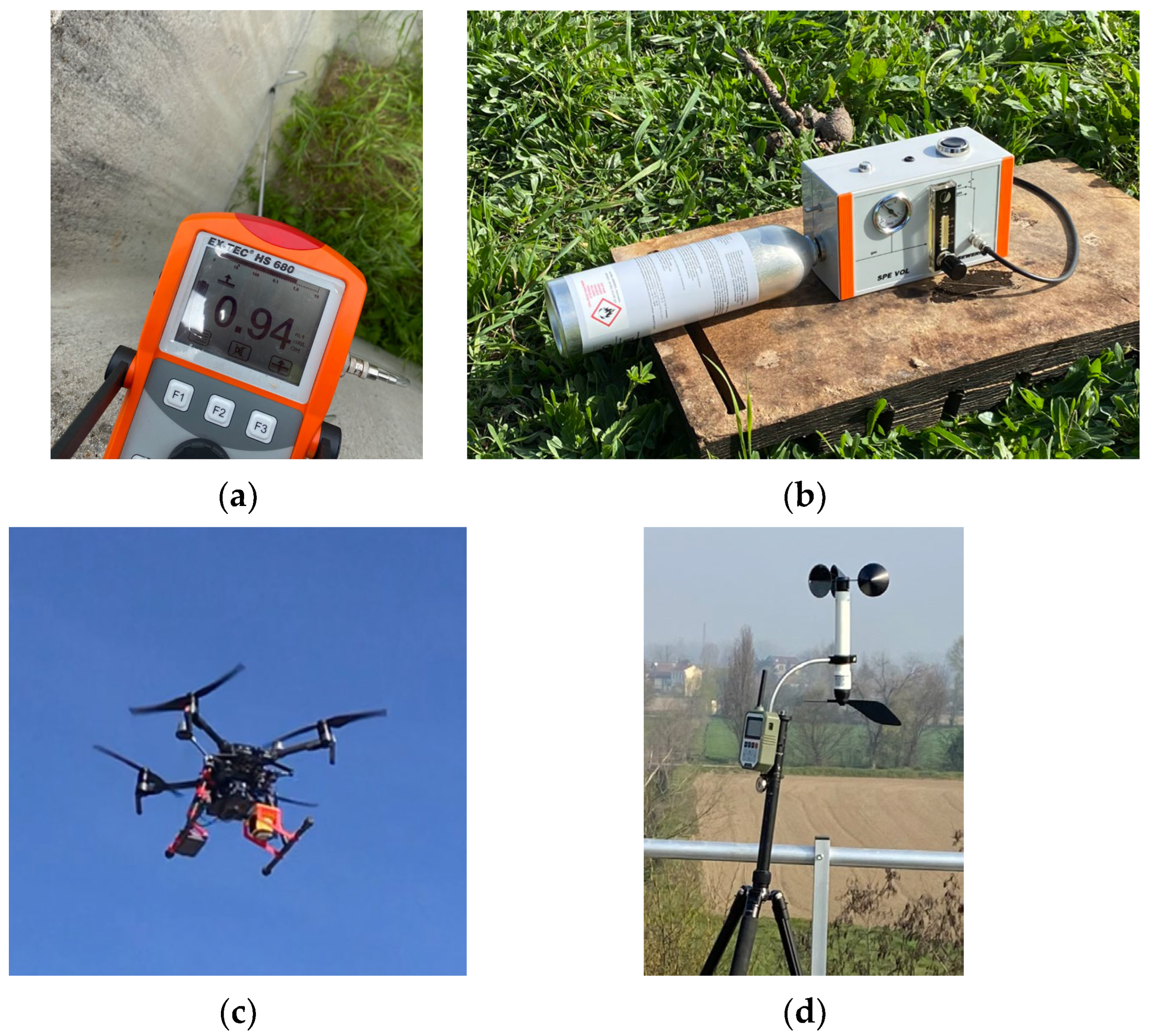

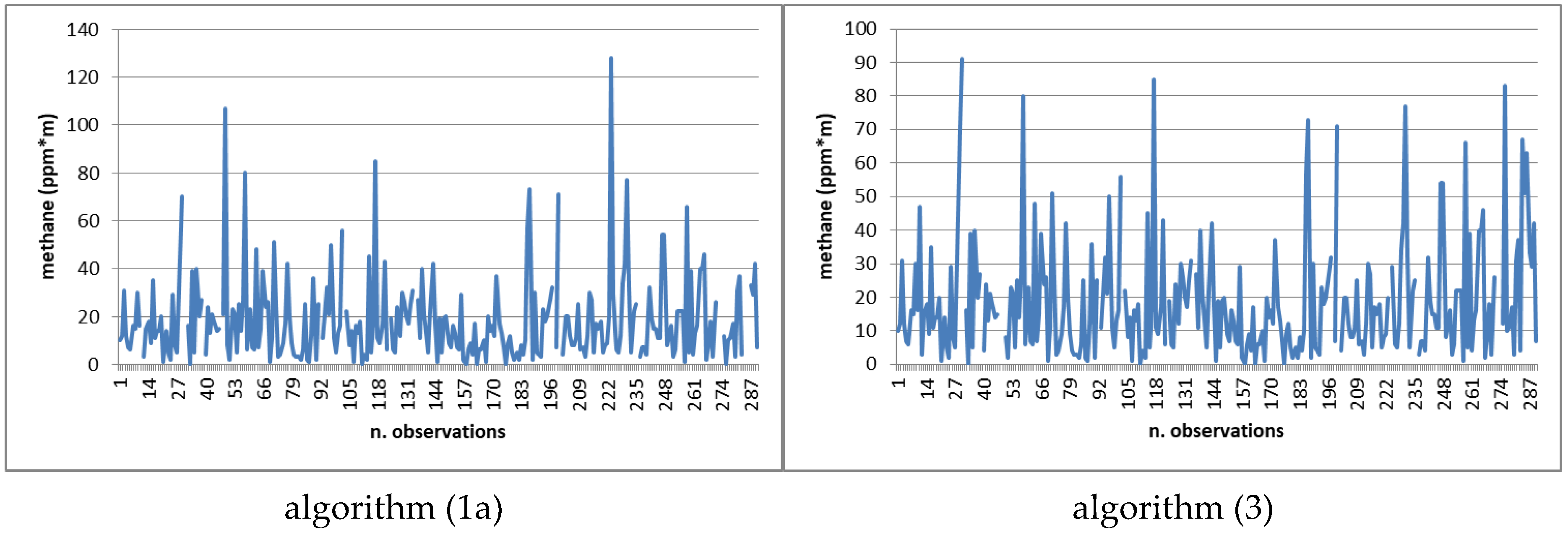
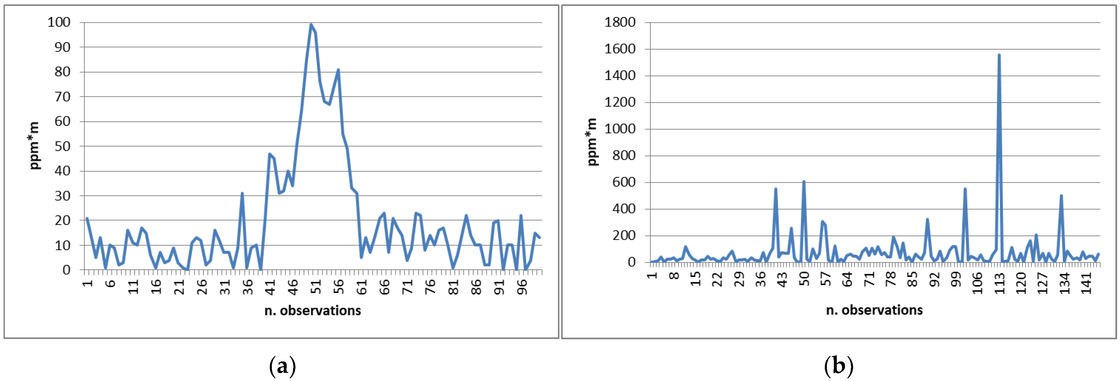
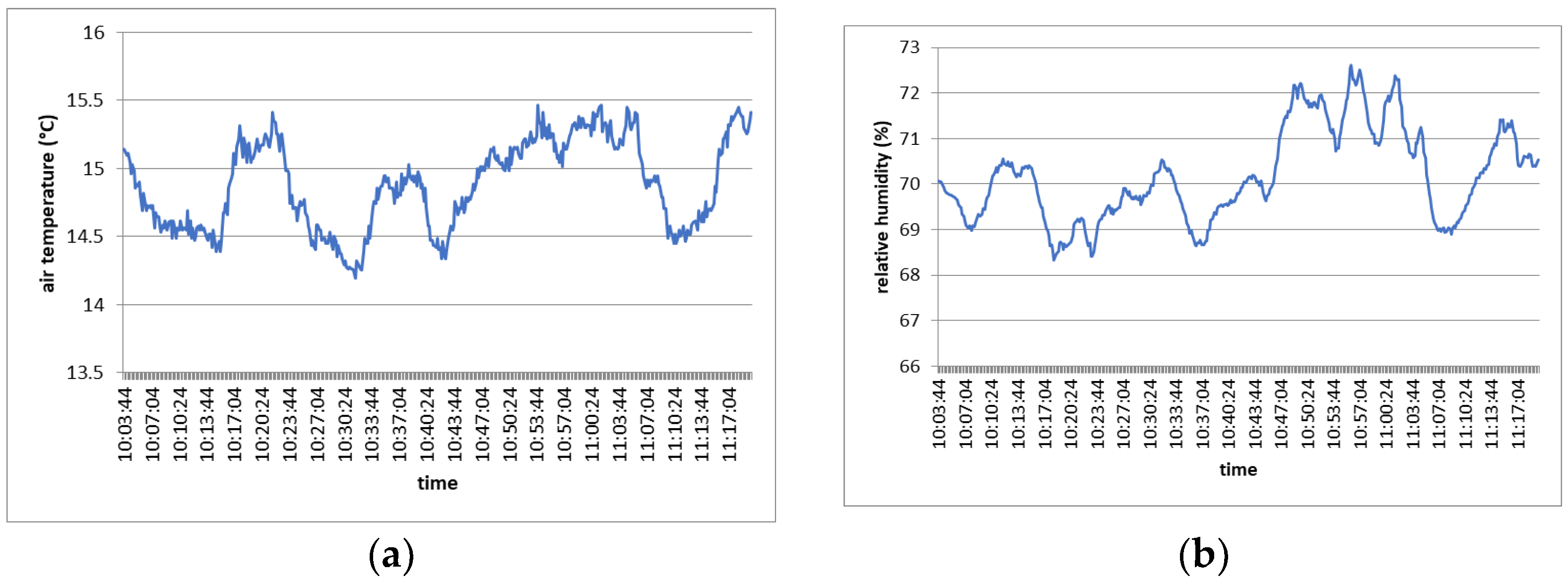

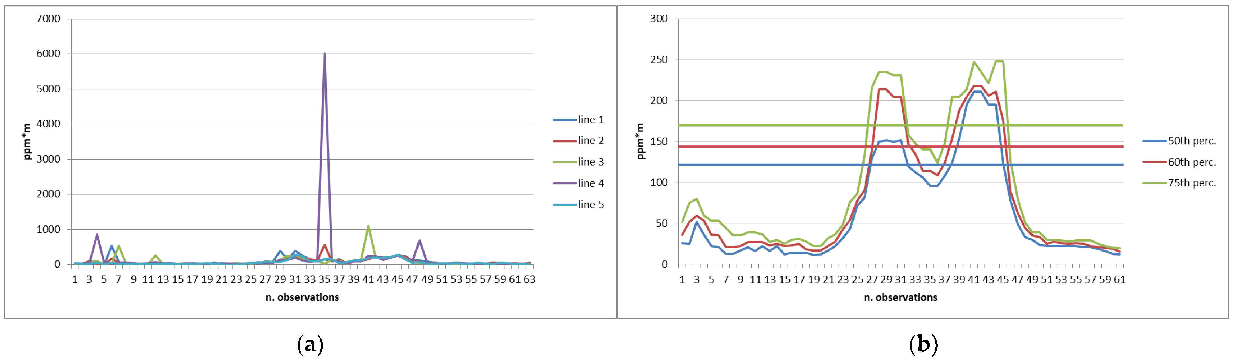
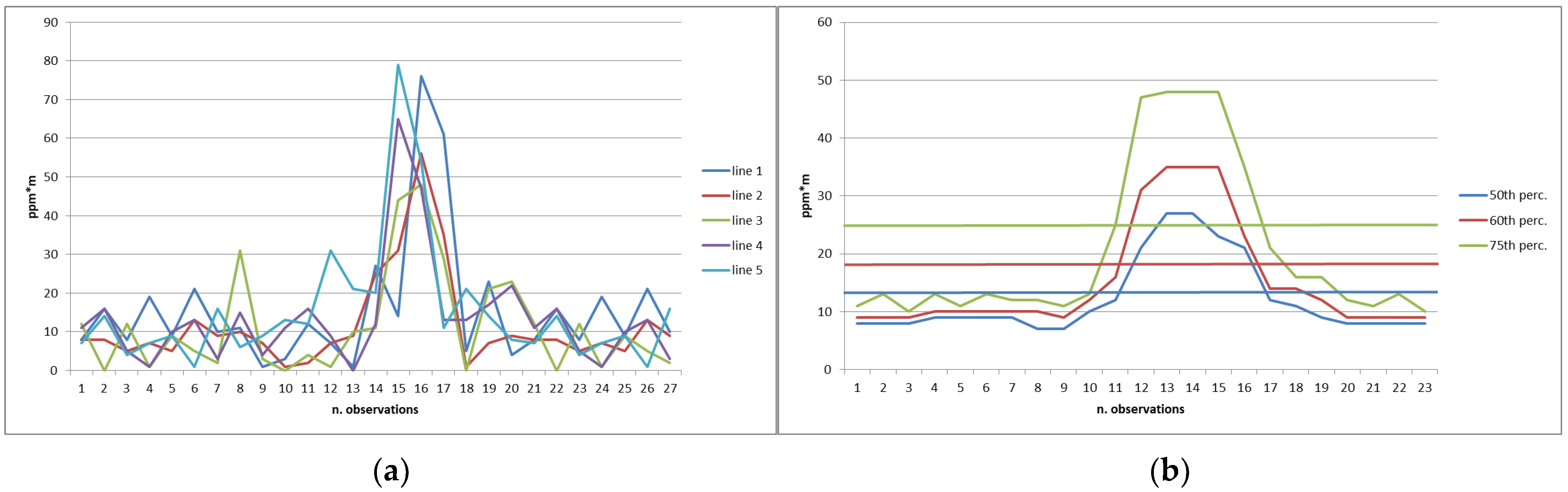
Disclaimer/Publisher’s Note: The statements, opinions and data contained in all publications are solely those of the individual author(s) and contributor(s) and not of MDPI and/or the editor(s). MDPI and/or the editor(s) disclaim responsibility for any injury to people or property resulting from any ideas, methods, instructions or products referred to in the content. |
© 2025 by the authors. Licensee MDPI, Basel, Switzerland. This article is an open access article distributed under the terms and conditions of the Creative Commons Attribution (CC BY) license (https://creativecommons.org/licenses/by/4.0/).