An Adaptive Electric Vehicle Charging Management Strategy for Multi-Level Travel Demands


Abstract
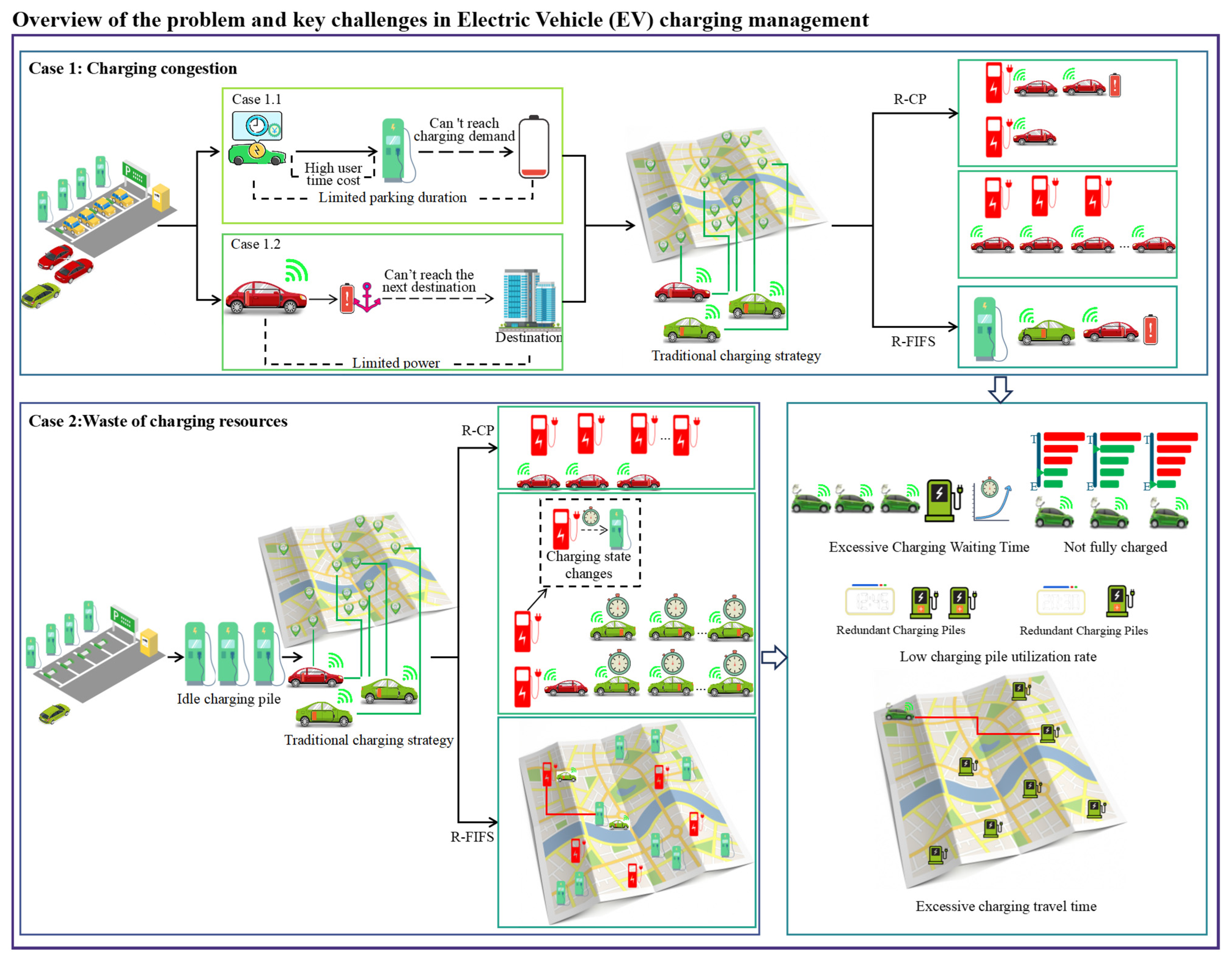
:1. Introduction
2. Scheduling Strategy for Reserved Vehicles
2.1. Charging Priority Parameter Calculation Model
2.1.1. Attention Mechanism
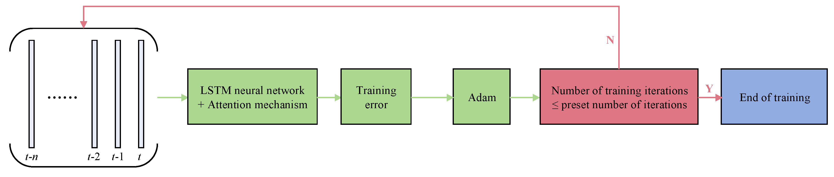
2.1.2. Attention-LSTM Model
- (1)
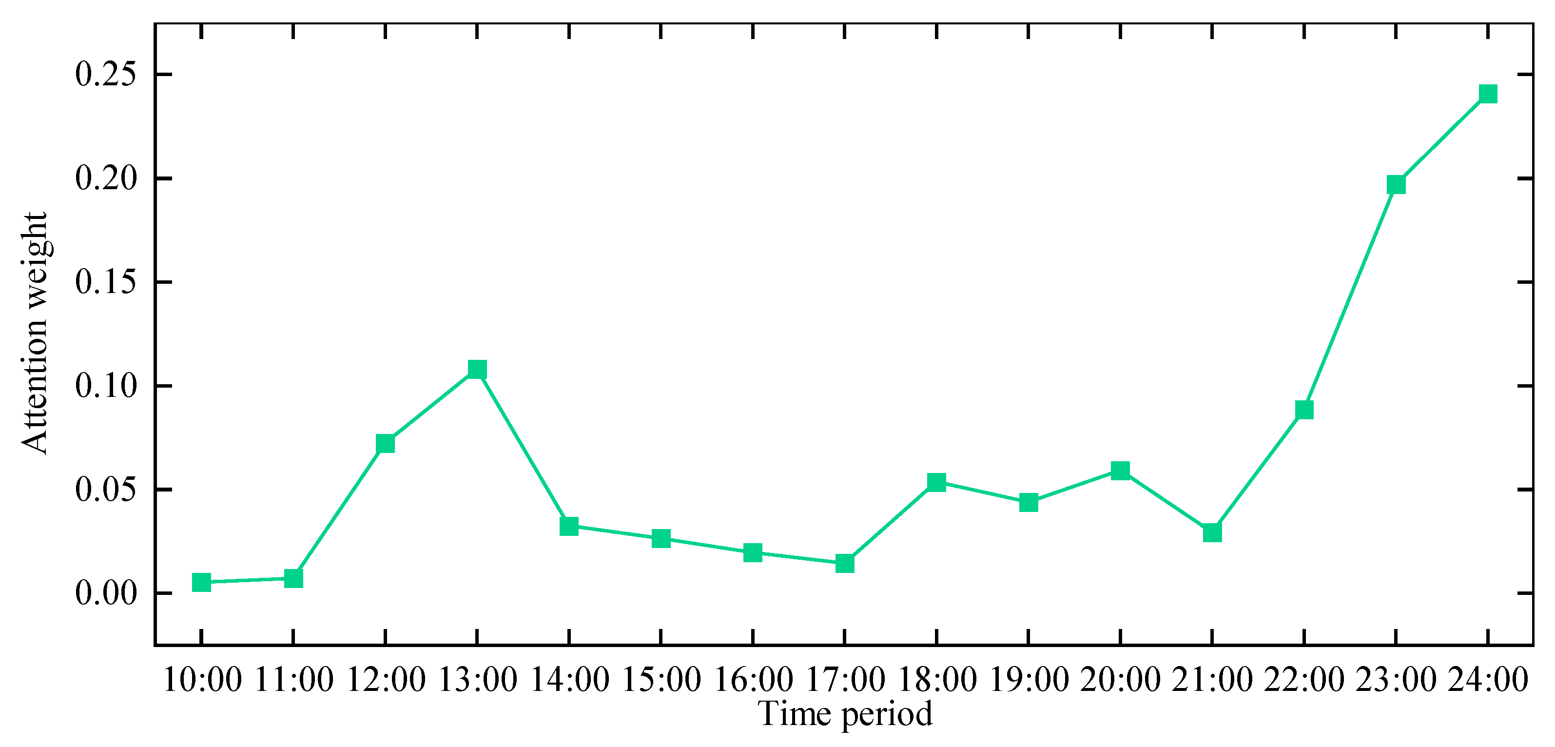
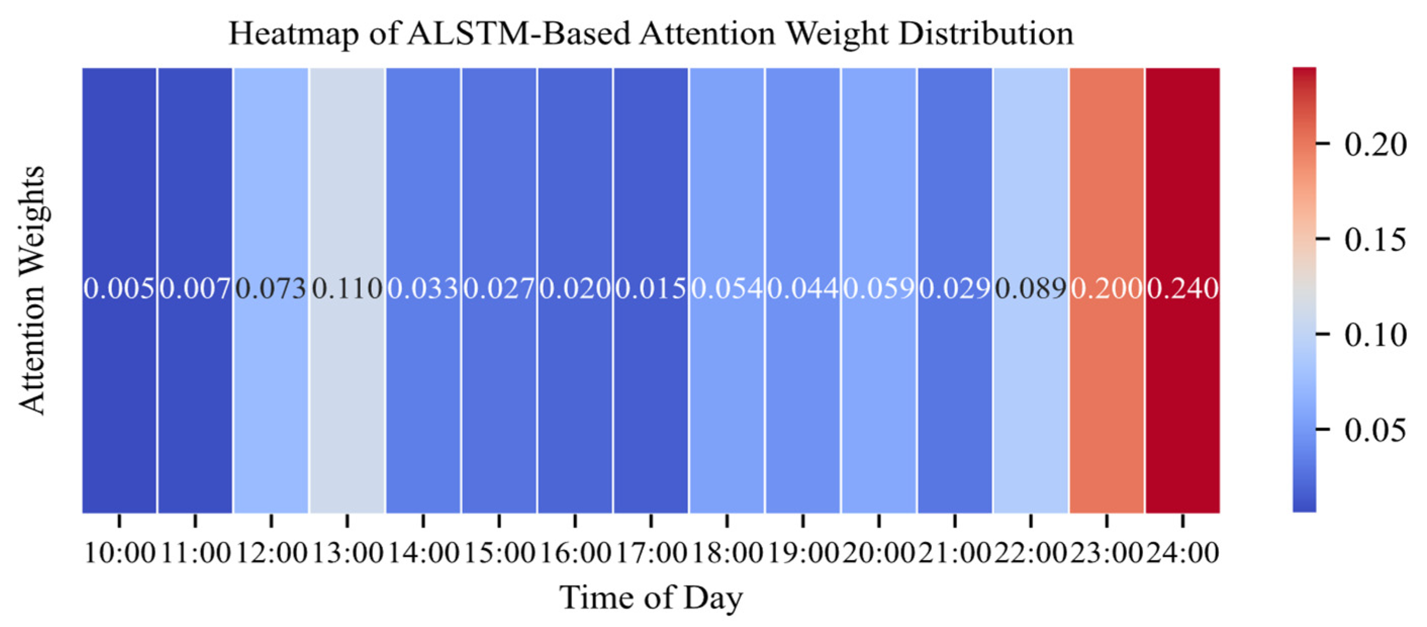
- Late-night high charging demand period (23:00–24:00, 22:00): During the late-night period, especially from 23:00 to 24:00, vehicle arrival rates significantly increase as many users charge their vehicles after parking to ensure their travel needs for the following day. During this period, Attention-LSTM assigns higher attention weights to improve the prediction accuracy of late-night vehicle arrival behavior.
- (2)
- Midday short-term charging peak period (12:00–14:00): During the lunch break, there is a short-term surge in vehicle arrivals. Attention-LSTM focuses on the short-term high-frequency arrival patterns, ensuring accurate prediction of vehicles’ arrival rates during this brief peak period.
- (3)
- Evening rush hour and load fluctuation period (18:00–20:00, 16:00–17:00): During the evening commute, charging station utilization rises dramatically, leading to a sudden spike in charging demand. Attention-LSTM dynamically adjusts its attention allocation during these periods to accurately predict vehicle arrival fluctuations during the evening rush.
- (4)
- Low-load but highly volatile periods (10:00–11:00, 15:00, 21:00): Although the overall arrival rate during these periods is low, there are fluctuations in the arrival rates of some high-priority vehicles, especially around 21:00, when some users prepare for nighttime charging. Attention-LSTM allocates attention weights moderately to avoid overfocusing on non-critical periods while capturing potential abnormal fluctuations.
2.2. Algorithm for Reserving Charging Piles for Selection
3. Non-Reservation Vehicle Scheduling Strategy
3.1. Optimization Model of Scheduling Strategy
3.2. Optimization Algorithm
4. Reservation Vehicle and Charging Pile Matching Algorithm
4.1. Reservation Vehicle and Charging Pile Matching Model
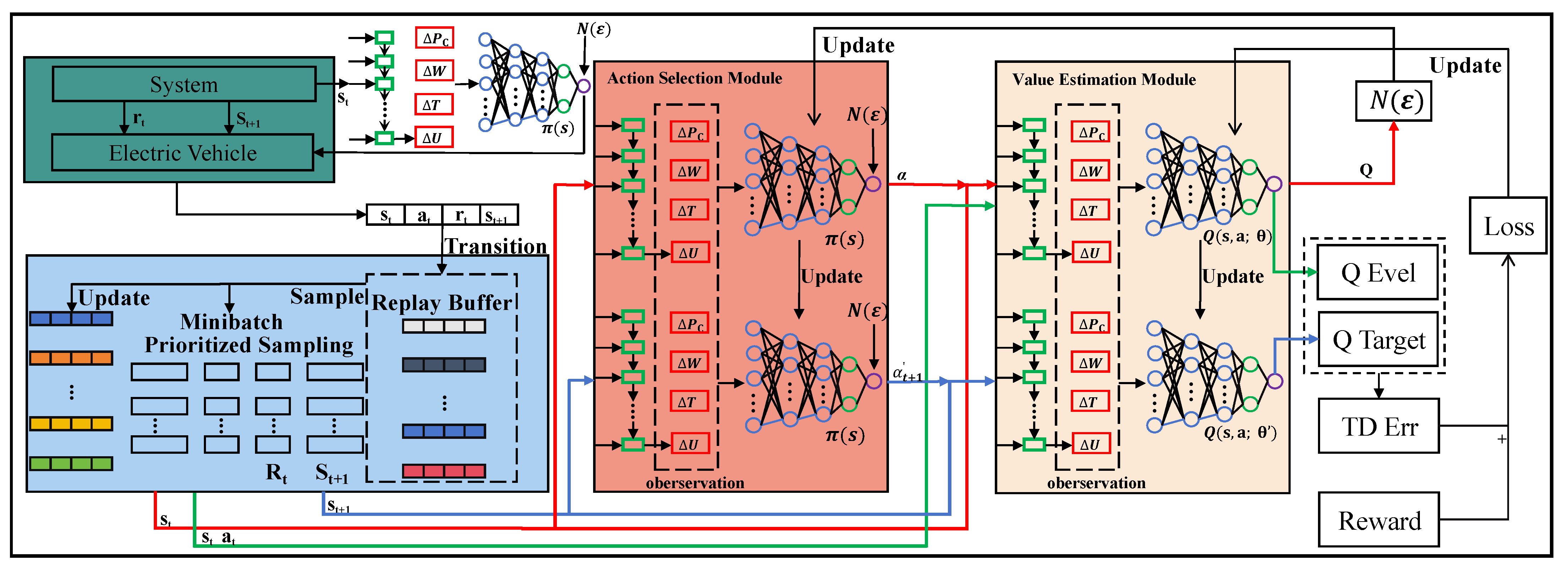
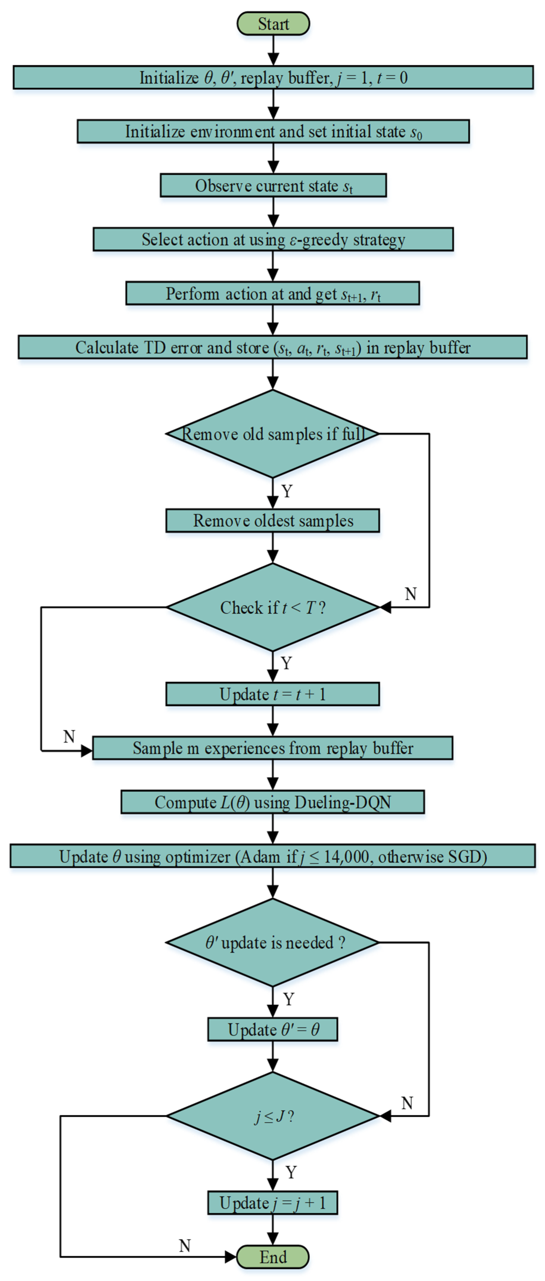
4.2. Vehicle and Charging Pile Matching Framework
| Algorithm 1: Reservation Vehicle and Charging Pile Matching Algorithm (DDPDQN) | |
| Input: State space S (system dynamic states, queue lengths, SOC thresholds, etc.), Action space A (actions such as assigning reserved piles, adjusting non-reserved resources), (immediate feedback for evaluating the action), Replay buffer D with capacity M, Discount factor , exploration rate , initial parameters Batch size m, learning rate Output: Optimized policy for matching vehicles to charging piles | |
| 1 | Step 1: Initialization |
| 2 | Initialize replay buffer D with capacity M; |
| 3 | Initialize Dueling DQN network with random parameters ; |
| 4 | Initialize target network with parameters ←; |
| 5 | ; |
| 6 | Set learning rate for gradient descent; |
| 7 | Initialize counters for training iterations k ← 0; |
| 8 | Note: Ensure input state dimension is derived from system observations based on 2.1. |
| 9 | Step 2: System Initialization |
| 10 | , including: |
| 11 | ; |
| 12 | for high/low priority vehicles; |
| 13 | ; |
| 14 | ; |
| 15 | ; |
| 16 | , incorporating inputs from 2.1 and 2.2; |
| 17 | Step 3: Interaction with Environment |
| 18 | for each time step t do |
| 19 |
using -greedy strategy: . Note: Ensure input state dimension is derived from system observations based on 2.1; |
| 20 | ; |
| 21 | ; |
| 22 | in replay buffer D; |
| 23 | if |D| > M then |
| 24 | Remove oldest transition from D; |
| 25 | end |
| 26 | Note: incorporates system-level performance metrics such as waiting time reduction (from 3) and load balancing (from 2.2); |
| 27 | end |
| 28 | Step 4: Prioritized Experience Replay |
| 29 | Priority Calculation:: : Batch Sampling:, prioritizing samples with higher TD errors from 2.1 and 2.2; |
| 30 | Step 5: Model Training |
| 31 | Compute the loss function for the minibatch: Use gradient descent to update network parameters : Note: Loss function incorporates feedback from 2.1 and 3 through rewards ; |
| 32 | Step 6: Dueling DQN Update |
| 33 | : Every fixed number of steps synchronizes target network parameters: |
| 34 | Step 7: Exploration Rate Decay |
| 35 | Update exploration rate ε:
. is the total decay steps; |
| 36 | Increment training counter k←k + 1; |
| 37 | Step 8: Convergence Check |
| 38 | Repeat Steps 3 to 7 until policy converges to optimal strategy; |
| 39 | return Optimized policy for matching vehicles to charging piles |
5. Simulation Experiments and Analysis
5.1. Simulation Scenario Setup
- (1)
- Dynamic Priority Adjustment vs. Static Scheduling: The ACP strategy, by dynamically adjusting priorities, resource allocation, and non-reservation vehicle scheduling, offers greater flexibility in responding to fluctuations in charging demand compared to the static scheduling methods of FIFS and RFWDA. Both FIFS and RFWDA rely on static rules, which lack dynamic responsiveness to changing charging demand, leading to inefficient resource allocation.
- (2)
- Dynamic Charging Pile Allocation vs. Static Reservation Allocation: The ACP strategy not only prioritizes the needs of reserved vehicles but also includes a dedicated non-reservation vehicle scheduling strategy. This strategy assigns non-reservation vehicles to stations with lighter loads, reducing waiting times and improving resource utilization. In contrast, FIFS and RFWDA feature relatively simple scheduling mechanisms for non-reservation vehicles. FIFS treats all vehicles equally, while RFWDA prioritizes reserved vehicles but applies static scheduling for non-reservation vehicles, lacking dynamic optimization of resource distribution.
- (3)
- Non-Reservation Vehicle Scheduling Strategy: The ACP strategy features a non-reservation vehicle scheduling optimization strategy that dynamically allocates these vehicles to charging stations with lighter loads based on station load and non-reservation vehicle arrival rates, preventing queuing issues during peak demand periods. In comparison, FIFS and RFWDA lack dedicated scheduling mechanisms for non-reservation vehicles, with scheduling relying entirely on arrival order or static rules, unable to flexibly respond to demand fluctuations.
- (4)
- Charging Resource Matching Mechanism: The ACP strategy dynamically matches charging piles with reservation vehicles using the DDPDQN algorithm, which can adjust resource allocation in real time to respond to load fluctuations and demand changes. In contrast, FIFS and RFWDA do not account for the impact of load fluctuations on resource allocation, and their charging pile matching is more rigid and lacks flexibility.
- (1)
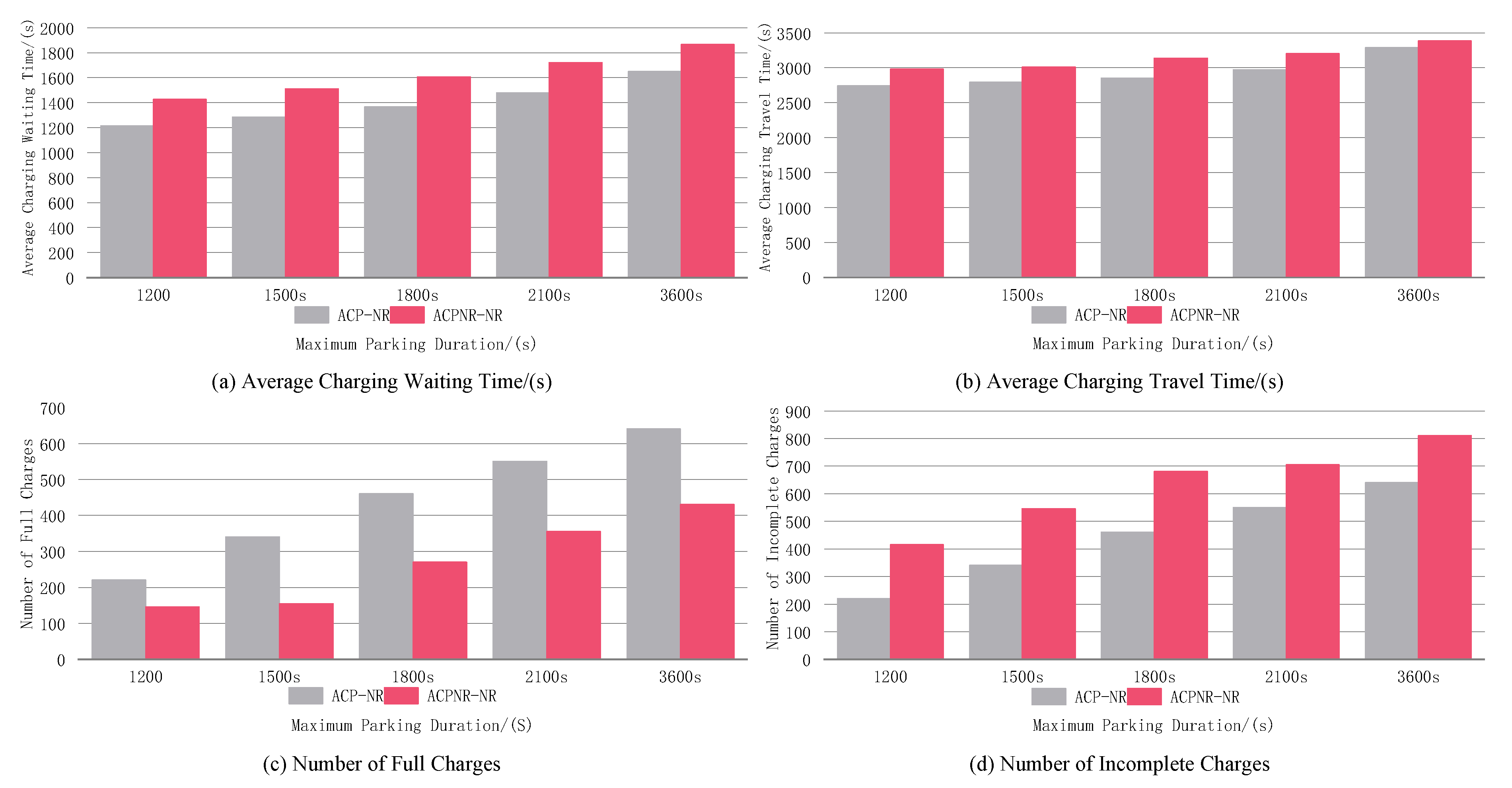
- Average Charging Waiting Time: The average time users wait from arriving at a charging station to starting to charge, reflecting the timeliness of charging services.
- (2)
- Average Charging Travel Time: The total time from departure to charging completion, including travel, waiting, and charging times, representing overall charging efficiency.
- (3)
- Full Charging Count: The number of instances where vehicles achieved a full charge within the allowed parking time, indicating the efficiency of resource utilization.
- (4)
- Unfinished Charging Count: The number of instances where vehicles failed to fully charge due to parking time constraints, including cases where users were still waiting to charge when the parking limit was reached.
5.2. High-Priority Vehicle Arrival Rate Prediction: Experiments and Analysis
5.2.1. Dataset
5.2.2. Training Phase Analysis
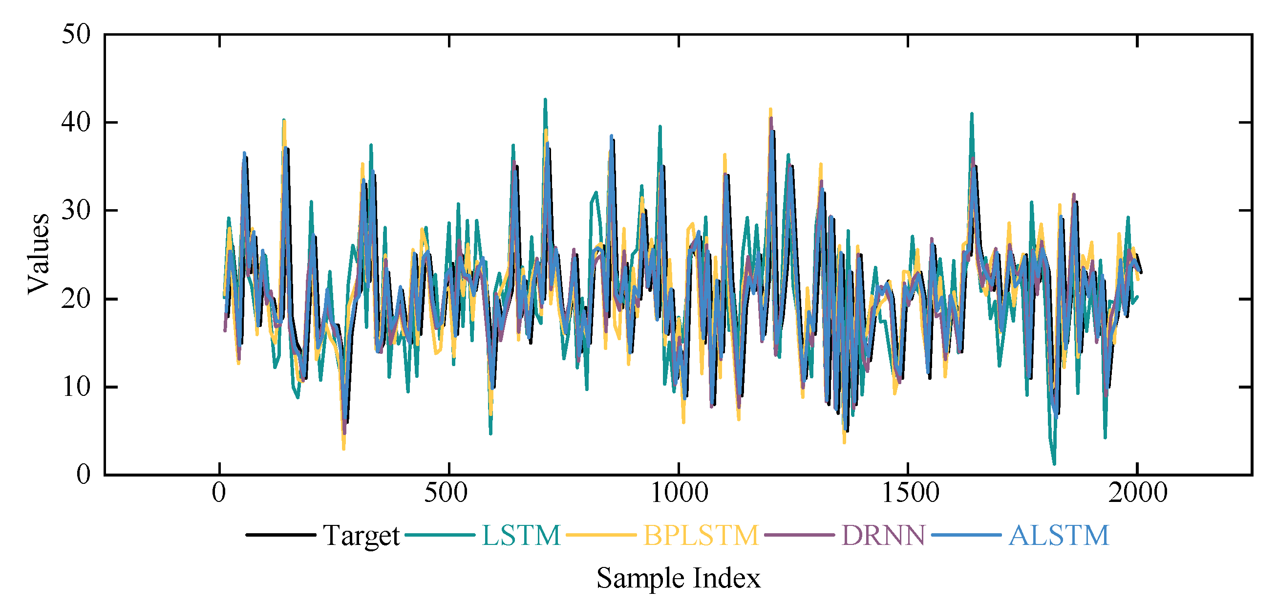
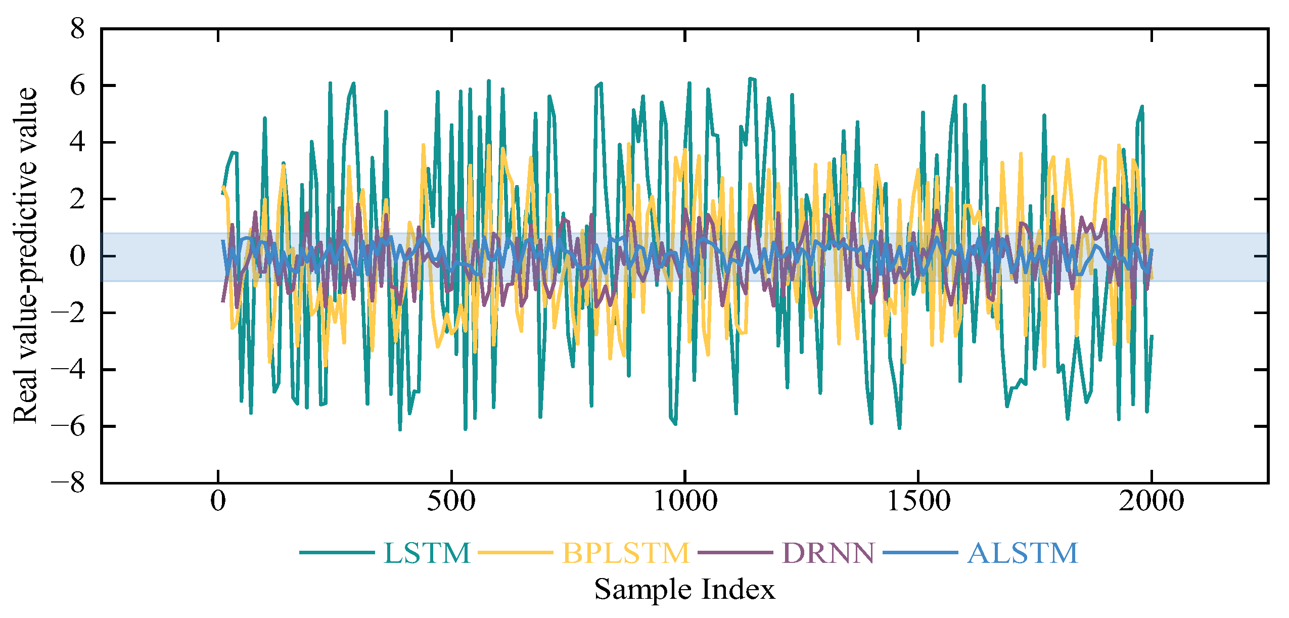
5.2.3. Experimental Analysis in the Testing Phase
5.3. Impact of Reserved Charging Piles: Experiment and Analysis
5.4. Reserved Vehicle and Charging Pile Matching: Experiment and Results Analysis
5.5. Validation of Charging Efficiency Results
5.6. Model Parameter Impact Analysis
6. Conclusions
Author Contributions
Funding
Institutional Review Board Statement
Informed Consent Statement
Data Availability Statement
Conflicts of Interest
References
- Liu, Z.; Song, J.; Kubal, J.; Susarla, N.; Knehr, K.W.; Islam, E.; Nelson, P.; Ahmed, S. Comparing total cost of ownership of battery electric vehicles and internal combustion engine vehicles. Energy Policy 2021, 158, 112564. [Google Scholar] [CrossRef]
- Sun, C.X.; Li, T.X.; Tang, X.Y. A Data-Driven Approach for Optimizing Early-Stage Electric Vehicle Charging Station Placement. IEEE Trans. Ind. Inform. 2024, 20, 11500–11510. [Google Scholar] [CrossRef]
- Habbal, A.; Alrifaie, M.F. A User-Preference-Based Charging Station Recommendation for Electric Vehicles. IEEE Trans. Intell. Transp. Syst. 2024, 25, 11617–11634. [Google Scholar] [CrossRef]
- Infante, W.; Ma, J. Coordinated Management and Ratio Assessment of Electric Vehicle Charging Facilities. IEEE Trans. Ind. Appl. 2020, 56, 5955–5962. [Google Scholar] [CrossRef]
- Paudel, A.; Hussain, S.A.; Sadiq, R.; Zareipour, H.; Hewage, K. Decentralized cooperative approach for electric vehicle charging. J. Clean. Prod. 2022, 364, 132590. [Google Scholar] [CrossRef]
- International Energy Agency (IEA). Available online: https://www.iea.org/reports/global-ev-outlook-2024 (accessed on 22 February 2025).
- Chen, X.; Zhang, H.; Xu, Z.; Nielsen, C.P.; McElroy, M.B.; Lv, J. Impacts of Fleet Types and Charging Modes for Electric Vehicles on Emissions under Different Penetrations of Wind Power. Nat. Energy 2018, 3, 413–421. [Google Scholar] [CrossRef]
- Bilsalget i Desember og Hele 2024, Opplysningsrådet for Veitrafikken (OFV). Available online: https://ofv.no/bilsalget/bilsalget-i-desember-2024 (accessed on 22 February 2025).
- Sivertsgård, A.; Fjær, K.K.; Gogia, R.; Moum, A.L.; Sivertsgård, A.; Spilde, D.; Syrstad, T.A.; Tveten, Å.G.; Veie, C.A. Norsk og Nordisk Effektbalanse mot 2035; Norges Vassdrags- og Energidirektorat (NVE): Oslo, Norway, 2024; pp. 1–50. [Google Scholar]
- Chen, J.; Huang, X.Q.; Cao, Y.J.; Li, L.Y.; Yan, K.; Wu, L.; Liang, K. Electric vehicle charging schedule considering shared charging pile based on Generalized Nash Game. Int. J. Electr. Power Energy Syst. 2022, 136, 107579. [Google Scholar] [CrossRef]
- Amini, M.H.; Moghaddam, M.P.; Karabasoglu, O. Simultaneous allocation of electric vehicles’ parking lots and distributed renewable resources in smart power distribution networks. Sustain. Cities Soc. 2017, 28, 332–342. [Google Scholar] [CrossRef]
- Bandpey, M.F.; Firouzjah, K.G. Two-stage charging strategy of plug-in electric vehicles based on fuzzy control. Comput. Oper. Res. 2018, 96, 236–243. [Google Scholar] [CrossRef]
- Xydas, E.; Marmaras, C.; Cipcigan, L.M. A multi-agent based scheduling algorithm for adaptive electric vehicles charging. Appl. Energy 2016, 177, 354–365. [Google Scholar] [CrossRef]
- Abdalrahman, A.; Zhuang, W.H. Dynamic Pricing for Differentiated PEV Charging Services Using Deep Reinforcement Learning. IEEE Trans. Intell. Transp. Syst. 2022, 23, 1415–1427. [Google Scholar] [CrossRef]
- Bitar, E.; Xu, Y.J. Deadline Differentiated Pricing of Deferrable Electric Loads. IEEE Trans. Smart Grid 2017, 8, 13–25. [Google Scholar] [CrossRef]
- Huang, A.L.; Mao, Y.X.; Chen, X.S.; Xu, Y.H.; Wu, S.X. A multi-timescale energy scheduling model for microgrid embedded with differentiated electric vehicle charging management strategies. Sustain. Cities Soc. 2024, 101, 105123. [Google Scholar] [CrossRef]
- Flocea, R.; Hîncu, A.; Robu, A.; Senocico, S.; Traciu, A.; Remus, B.M.; Raboaca, M.S.; Filote, C. Electric Vehicle Smart Charging Reservation Algorithm. Sensors 2022, 22, 2834. [Google Scholar] [CrossRef]
- Cao, Y.; Jiang, T.; Kaiwartya, O.; Sun, H.J.; Zhou, H.; Wang, R. Toward Pre-Empted EV Charging Recommendation Through V2V-Based Reservation System. IEEE Trans. Syst. Man Cybern.-Syst. 2021, 51, 3026–3039. [Google Scholar] [CrossRef]
- Shen, X.X.; Lv, J.; Du, S.C.; Deng, Y.F.; Liu, M.L.; Zhou, Y.L. Integrated optimization of electric vehicles charging location and allocation for valet charging service. Flex. Serv. Manuf. J. 2024, 36, 1080–1106. [Google Scholar] [CrossRef]
- Lai, Z.J.; Li, S. On-demand valet charging for electric vehicles: Economic equilibrium, infrastructure planning and regulatory incentives. Transp. Res. Part C-Emerg. Technol. 2022, 140, 103669. [Google Scholar] [CrossRef]
- Shang, Y.T.; Li, Z.K.; Li, S.; Shao, Z.Y.; Jian, L.N. An Information Security Solution for Vehicle-to-Grid Scheduling by Distributed Edge Computing and Federated Deep Learning. IEEE Trans. Ind. Appl. 2024, 60, 4381–4395. [Google Scholar] [CrossRef]
- Jin, J.L.; Xu, Y.J. Optimal Policy Characterization Enhanced Actor-Critic Approach for Electric Vehicle Charging Scheduling in a Power Distribution Network. IEEE Trans. Smart Grid 2021, 12, 1416–1428. [Google Scholar] [CrossRef]
- Sadreddini, Z.; Guner, S.; Erdinc, O. Design of a Decision-Based Multicriteria Reservation System for the EV Parking Lot. IEEE Trans. Transp. Electrif. 2021, 7, 2429–2438. [Google Scholar] [CrossRef]
- Sone, S.P.; Lehtomaki, J.J.; Khan, Z.; Umebayashi, K.; Kim, K.S. Robust EV Scheduling in Charging Stations Under Uncertain Demands and Deadlines. IEEE Trans. Intell. Transp. Syst. 2024, 25, 21484–21499. [Google Scholar] [CrossRef]
- Ahmad, A.; Ullah, Z.; Khalid, M.; Ahmad, N. Toward Efficient Mobile Electric Vehicle Charging under Heterogeneous Battery Switching Technology. Appl. Sci. 2022, 12, 904. [Google Scholar] [CrossRef]
- Bao, Z.Y.; Xie, C. Optimal station locations for en-route charging of electric vehicles in congested intercity networks: A new problem formulation and exact and approximate partitioning algorithms. Transp. Res. Part C-Emerg. Technol. 2021, 133, 103447. [Google Scholar] [CrossRef]
- Madaram, V.; Biswas, P.K.; Sain, C.; Thanikanti, S.B.; Selvarajan, S. Optimal electric vehicle charge scheduling algorithm using war strategy optimization approach. Sci. Rep. 2024, 14, 21795. [Google Scholar] [CrossRef] [PubMed]
- Attaianese, C.; Di Pasquale, A.; Franzese, P.; Iannuzzi, D.; Pagano, M.; Ribera, M. A model-based EVs charging scheduling for a multi-slot Ultra-Fast Charging Station. Electr. Power Syst. Res. 2023, 216, 109009. [Google Scholar] [CrossRef]
- Deng, X.S.; Zhang, Q.; Li, Y.; Sun, T.; Yue, H.Z. Hierarchical Distributed Frequency Regulation Strategy of Electric Vehicle Cluster Considering Demand Charging Load Optimization. IEEE Trans. Ind. Appl. 2022, 58, 720–731. [Google Scholar] [CrossRef]
- Kim, B.; Paik, M.; Kim, Y.; Ko, H.; Pack, S. Distributed Electric Vehicle Charging Mechanism: A Game-Theoretical Approach. IEEE Trans. Veh. Technol. 2022, 71, 8309–8317. [Google Scholar] [CrossRef]
- Wang, Z.F.; Jochem, P.; Fichtner, W. A scenario-based stochastic optimization model for charging scheduling of electric vehicles under uncertainties of vehicle availability and charging demand. J. Clean. Prod. 2020, 254, 119886. [Google Scholar] [CrossRef]
- Das, S.; Thakur, P.; Singh, A.K.; Singh, S.N. Optimal management of vehicle-to-grid and grid-to-vehicle strategies for load profile improvement in distribution system. J. Energy Storage 2022, 49, 104068. [Google Scholar] [CrossRef]
- Wu, X.M.; Feng, Q.J.; Bai, C.C.; Lai, C.S.; Jia, Y.W.; Lai, L.L. A novel fast-charging stations locational planning model for electric bus transit system. Energy 2021, 224, 120106. [Google Scholar] [CrossRef]
- Ji, C.L.; Liu, Y.B.; Lyu, L.; Li, X.C.; Liu, C.; Peng, Y.X.; Xiang, Y. A Personalized Fast-Charging Navigation Strategy Based on Mutual Effect of Dynamic Queuing. IEEE Trans. Ind. Appl. 2020, 56, 5729–5740. [Google Scholar] [CrossRef]
- Qin, J.X.; Qiu, J.; Chen, Y.T.; Wu, T.; Xiang, L.G. Charging Stations Selection Using a Graph Convolutional Network from Geographic Grid. Sustainability 2022, 14, 16797. [Google Scholar] [CrossRef]
- Scarpelli, C.; Ceraolo, M.; Crisostomi, E.; Apicella, V.; Pellegrini, G. Charging Electric Vehicles on Highways: Challenges and Opportunities. IEEE Access 2024, 12, 55814–55823. [Google Scholar] [CrossRef]
- Tanwar, S.; Kakkar, R.; Gupta, R.; Raboaca, M.S.; Sharma, R.; Alqahtani, F.; Tolba, A. Blockchain-based electric vehicle charging reservation scheme for optimum pricing. Int. J. Energy Res. 2022, 46, 14994–15007. [Google Scholar] [CrossRef]
- Liu, S.H.; Ni, Q.; Cao, Y.; Cui, J.X.; Tian, D.X.; Zhuang, Y. A Reservation-Based Vehicle-to-Vehicle Charging Service Under Constraint of Parking Duration. IEEE Syst. J. 2023, 17, 176–187. [Google Scholar] [CrossRef]
- Xiao, Q.; Zhang, R.T.; Wang, Y.C.; Shi, P.; Wang, X.; Chen, B.R.; Fan, C.W.; Chen, G. A deep reinforcement learning based charging and discharging scheduling strategy for electric vehicles. Energy Rep. 2024, 12, 4854–4863. [Google Scholar] [CrossRef]
- Liu, L.F.; Huang, Z.; Xu, J. Multi-Agent Deep Reinforcement Learning Based Scheduling Approach for Mobile Charging in Internet of Electric Vehicles. IEEE Trans. Mob. Comput. 2024, 23, 10130–10145. [Google Scholar] [CrossRef]
- Zhang, Y.Y.; Rao, X.P.; Liu, C.Y.; Zhang, X.B.; Zhou, Y. A cooperative EV charging scheduling strategy based on double deep Q-network and Prioritized experience replay. Eng. Appl. Artif. Intell. 2023, 118, 105642. [Google Scholar] [CrossRef]
- Wang, L.; Hou, L.Y.; Liu, S.X.; Han, Z.; Wu, J. Reinforcement Contract Design for Vehicular-Edge Computing Scheduling and Energy Trading via Deep Q-Network With Hybrid Action Space. IEEE Trans. Mob. Comput. 2024, 23, 6770–6784. [Google Scholar] [CrossRef]
- Li, F.; Zuo, W.; Zhou, K.; Li, Q.Q.; Huang, Y.H.; Zhang, G.D. State-of-charge estimation of lithium-ion battery based on second order resistor-capacitance circuit-PSO-TCN model. Energy 2024, 289, 130025. [Google Scholar] [CrossRef]
- Li, F.; Zuo, W.; Zhou, K.; Li, Q.Q.; Huang, Y.H. State of charge estimation of lithium-ion batteries based on PSO-TCN-Attention neural network. J. Energy Storage 2024, 84, 110806. [Google Scholar] [CrossRef]
- Srivastava, N.; Hinton, G.; Krizhevsky, A.; Sutskever, I.; Salakhutdinov, R. Dropout: A simple way to prevent neural networks from overfitting. J. Mach. Learn. Res. 2014, 15, 1929–1958. [Google Scholar]
- Kingma, D.P.; Ba, J. Adam: A method for stochastic optimization. In Proceedings of the 3rd International Conference on Learning Representations (ICLR), San Diego, CA, USA, 7–9 May 2015. [Google Scholar]
- Kirkpatrick, S.; Gelatt, C.D., Jr.; Vecchi, M.P. Optimization by simulated annealing. Science 1983, 220, 671–680. [Google Scholar] [CrossRef] [PubMed]
- Van Laarhoven, P.J.M.; Aarts, E.H.L. Simulated Annealing: Theory and Applications; Reidel: Dordrecht, The Netherlands, 1987; pp. 1–187. [Google Scholar]
- Mnih, V.; Kavukcuoglu, K.; Silver, D.; Rusu, A.A.; Veness, J.; Bellemare, M.G.; Graves, A.; Riedmiller, M.; Fidjeland, A.K.; Ostrovski, G.; et al. Human-level control through deep reinforcement learning. Nature 2015, 518, 529–533. [Google Scholar] [CrossRef]
- Schaul, T.; Quan, J.; Antonoglou, I.; Silver, D. Prioritized experience replay. In Proceedings of the 4th International Conference on Learning Representations (ICLR), San Juan, PR, USA, 2–4 May 2016. [Google Scholar]
- Hessel, M.; Modayil, J.; van Hasselt, H.; Schaul, T.; Ostrovski, G.; Dabney, W.; Horgan, D.; Piot, B.; Azar, M.G.; Silver, D. Rainbow: Combining Improvements in Deep Reinforcement Learning. In Proceedings of the Thirty-Second AAAI Conference on Artificial Intelligence, New Orleans, LA, USA, 2–7 February 2018. [Google Scholar]
- Hu, L.; Dong, J.; Lin, Z.H. Modeling charging behavior of battery electric vehicle drivers: A cumulative prospect theory based approach. Transp. Res. Part C-Emerg. Technol. 2019, 102, 474–489. [Google Scholar] [CrossRef]
- Tian, H.; Sun, Y.J.; Hu, F.F.; Du, J.Y. Charging Behavior Analysis Based on Operation Data of Private BEV Customers in Beijing. Electronics 2023, 12, 373. [Google Scholar] [CrossRef]


| Symbol | Variable Definition |
|---|---|
| Wij | Attention layer weight allocation factor |
| c | Feature vector |
| Sij | Scoring function |
| Weight factor | |
| Bias factor | |
| xt | Time step in the input sequence |
| ht | Intermediate state computed by LSTM |
| Predicted and actual arrival rates of high-priority vehicles | |
| N | Total sample size |
| Average value of the actual arrival rate of reserved vehicles | |
| Pc | Charging priority parameters |
| α | Normalized arrival rate deviation factor |
| β | Initial average arrival rate value |
| Total number of charging piles | |
| Number of reserved charging piles | |
| Emin, Emax | Minimum and maximum expected waiting times |
| μ | Service rate of a single charging pile |
| Load rate of high-priority vehicles at reserved charging piles | |
| Minimum and maximum constrained charging wait times | |
| Tavg | Average queue waiting time within the region |
| Average queue waiting times for high-priority (reserved) and low-priority vehicles | |
| Weight coefficient for the average queue waiting time of reserved vehicles versus random vehicles | |
| Upper and lower bounds of charging priority parameters | |
| Binary decision variable representing the reservation status of a charging pile | |
| j, k | Charging station and charging pile number |
| Service gain when charging pile k is allocated as a reserved charging pile | |
| Unit-time service value contributed by high-priority users | |
| Time occupied by high-priority users at charging pile k | |
| Unit-time resource consumption of charging pile k | |
| Queue length of high- and low-priority vehicles at charging station j at time t | |
| Number of temporarily allocated non-reserved charging piles at charging station j | |
| Number of non-reserved charging piles at charging station j | |
| Set of reserved charging piles at charging station j | |
| Set of temporarily allocated non-reserved charging piles at charging station j | |
| Decision variable for high- and low-priority users’ utilization of charging pile j | |
| Temporary allocation state decision variable for charging pile j | |
| Remaining number of charging piles at charging station j | |
| Arrival rate of random vehicles in subregion r | |
| Proportion of random vehicles in subregion r assigned to charging station j | |
| Queue waiting time of random vehicles at charging station j | |
| Probability of entering queue at charging station j | |
| Travel time from subregion r to charging station j | |
| Distance from subregion r to charging station j | |
| Average travel speed in subregion r | |
| P | Probability of accepting a new solution |
| Difference between the objective function value of the new solution and the current solution | |
| T0, T | Initial temperature and current temperature |
| α | Cooling factor |
| SOC threshold for high- and low-priority vehicles | |
| Charging pile status | |
| Current and next system states | |
| State transition probability | |
| Reward function | |
| Average charging wait time and travel time of users in the region | |
| Utilization rate of charging piles at charging stations in the region | |
| Charging wait time factor, charging travel time factor, and charging pile utilization factor | |
| ΔPc, ΔW, ΔT, ΔU | Charging priority parameter, changes in charging wait time, charging travel time, and charging pile utilization |
| Exploration rate at the k-th training iteration | |
| Random number in the range [0, 1] | |
| Initial and final exploration rates | |
| Total decay steps | |
| δi | TD error |
| P(i) | Experience sampling probability |
| α | Influence factor of prioritized sampling |
| β | Balancing factor for importance sampling weight |
| N | Size of the experience replay buffer |
| Target action | |
| QEval, QTarget | Evaluation and target Q-values |
| θ, θ′ | Target network parameters |
| m | Mini-batch sample size |
| L(θ) | Loss function value |
| J | Maximum training iterations |
| Set Size | MAE | R2 |
|---|---|---|
| 3 | 1.354 | 0.872 |
| 5 | 1.126 | 0.905 |
| 10 | 0.983 | 0.937 |
| 20 | 1.101 | 0.923 |
| Hyperparameter | Candidate Values |
|---|---|
| Time step | {3, 5, 10, 20} |
| Number of attention layer nodes | {64, 128, 256} |
| Hidden layer configuration | {Single Layer (128), Double Layer (128, 64), Triple Layer (256, 128, 64)} |
| Learning rate | {0.0005, 0.001, 0.005} |
| Batch size | {16, 32, 64} |
| Number of training epochs | {100, 200, 300} |
| Dropout rate | {0.2, 0.5} |
| Optimizer | Adam |
| Parameter Name | Value |
|---|---|
| Number of nodes in the attention layer | 128 |
| Time step | 10 |
| Training sequence ratio | 80% |
| Test sequence ratio | 20% |
| Batch size | 32 |
| Training round | 200 |
| Intermediate layer and number of nodes | Two floors (128, 64) |
| Activation function | ReLU |
| Optimizer | Adam |
| Learning rate | 0.001 |
| Number of dropout layers and ratio | One floor (0.2) |
| Parameter Name | Parameter Value |
|---|---|
| Initial temperature T0 | 100 |
| Cooling factor α | 7 |
| Temperature stopping threshold Tmin | 10−4 |
| Maximum number of iterations Kmax | 1000 |
| Neighborhood search range δα | ±0.01 |
| Parameter Name | Parameter Value |
|---|---|
| Number of hidden layer nodes | 128, 64, 32 |
| Initial optimizer/learning rate | Adam/0.001 |
| Post-optimizer/learning rate | SGD/0.0001 |
| Experience pool capacity | 10,000 |
| Batch size | 64 |
| TD error threshold (ε) | 200 |
| Initial exploration rate | 1.0 |
| Final exploration rate | 0.01 |
| Exploration rate decay step | 10,000 |
| Discount factor | 0.99 |
| Number of training rounds | 20,000 |
| Target network update frequency | 500 |
| Algorithm | MSE |
|---|---|
| LSTM | 3.876 |
| BPLSTM | 2.745 |
| DRNN | 1.173 |
| ALSTM | 0.238 |
| Algorithm | MAE | R2 |
|---|---|---|
| LSTM | 3.127 | 0.903 |
| BPLSTM | 2.014 | 0.935 |
| DRNN | 0.915 | 0.961 |
| ALSTM | 0.341 | 0.978 |
| Parameter Name | Parameter Value |
|---|---|
| Reservation vehicle arrival rate rh | 14/h–26/h |
| Random vehicle arrival rate rl | 9/h–14/h |
| Minimum queuing time | 15 min |
| Maximum queue waiting time | 45 min |
| waiting time balance factor between reserved and random vehicles φ | 10 |
| Individual charging post service rate (number of vehicles that can be served per unit of time) | 0.4/h |
| Charge Priority Parameters | Number of Piles Reserved | Minimum Desired Queue Waiting Time | Maximum Desired Queuing Time | Average Waiting Time in Queues in the Region |
|---|---|---|---|---|
| (1) rh = 14/h | ||||
| 0.05 | 1 | 14 | 30 | 22.1 |
| 0 | 0 | 15 | 31 | 23.3 |
| (2) rh = 16/h | ||||
| 0.057 | 2 | 14 | 30 | 23.4 |
| 0.007 | 1 | 15 | 31 | 23.4 |
| 0 | 0 | 16 | 32 | 24.2 |
| (3) rh = 18/h | ||||
| 0.065 | 2 | 15 | 31 | 25.9 |
| 0.015 | 1 | 16 | 32 | 25.6 |
| 0 | 0 | 17 | 33 | 26.7 |
| (4) rh = 20/h | ||||
| 0.071 | 2 | 16 | 32 | 28.7 |
| 0.021 | 1 | 17 | 33 | 28.1 |
| 0 | 0 | 18 | 34 | 28.4 |
| (5) rh = 22/h | ||||
| 0.077 | 2 | 17 | 33 | 32.5 |
| 0.027 | 1 | 18 | 34 | 30.3 |
| 0 | 0 | 19 | 35 | 31.7 |
| (6) rh = 24/h | ||||
| 0.082 | 2 | 18 | 34 | 38.6 |
| 0.032 | 1 | 19 | 35 | 34.2 |
| 0 | 0 | 20 | 36 | 33.1 |
| (7) rh = 26/h | ||||
| 0.086 | 2 | 19 | 35 | 46.7 |
| 0.036 | 1 | 20 | 36 | 39.4 |
| 0 | 0 | 21 | 37 | 36.8 |
Disclaimer/Publisher’s Note: The statements, opinions and data contained in all publications are solely those of the individual author(s) and contributor(s) and not of MDPI and/or the editor(s). MDPI and/or the editor(s) disclaim responsibility for any injury to people or property resulting from any ideas, methods, instructions or products referred to in the content. |
© 2025 by the authors. Licensee MDPI, Basel, Switzerland. This article is an open access article distributed under the terms and conditions of the Creative Commons Attribution (CC BY) license (https://creativecommons.org/licenses/by/4.0/).
Share and Cite
Zhang, S.; Guo, D.; Zhou, B.; Zheng, C.; Li, Z.; Ma, P. An Adaptive Electric Vehicle Charging Management Strategy for Multi-Level Travel Demands. Sustainability 2025, 17, 2501. https://doi.org/10.3390/su17062501
Zhang S, Guo D, Zhou B, Zheng C, Li Z, Ma P. An Adaptive Electric Vehicle Charging Management Strategy for Multi-Level Travel Demands. Sustainability. 2025; 17(6):2501. https://doi.org/10.3390/su17062501
Chicago/Turabian StyleZhang, Shuai, Dong Guo, Bin Zhou, Chunyan Zheng, Zhiqin Li, and Pengcheng Ma. 2025. "An Adaptive Electric Vehicle Charging Management Strategy for Multi-Level Travel Demands" Sustainability 17, no. 6: 2501. https://doi.org/10.3390/su17062501
APA StyleZhang, S., Guo, D., Zhou, B., Zheng, C., Li, Z., & Ma, P. (2025). An Adaptive Electric Vehicle Charging Management Strategy for Multi-Level Travel Demands. Sustainability, 17(6), 2501. https://doi.org/10.3390/su17062501