Abstract
The recent success of emission reduction policies in China has significantly lowered sulfur dioxide (SO2) levels. However, accurately forecasting these concentrations remains challenging due to their inherent non-stationary tendency. This study introduces an innovative hybrid deep learning model, RF-VMD-Seq2Seq, combining the Random Forest (RF) algorithm, Variational Mode Decomposition (VMD), and the Sequence-to-Sequence (Seq2Seq) framework to improve SO2 concentration forecasting in five coastal cities of northern China. Our results show that the predicted SO2 concentrations closely align with observed values, effectively capturing fluctuations, outliers, and extreme events—such as sharp declines the Novel Coronavirus Pneumonia (COVID-19) pandemic in 2020—along with the upper 5% of SO2 levels. The model achieved high coefficients of determination (>0.91) and Pearson’s correlation (>0.96), with low prediction errors (RMSE < 1.35 μg/m3, MAE < 0.94 μg/m3, MAPE < 15%). The low-frequency band decomposing from VMD showed a notable long-term decrease in SO2 concentrations from 2013 to 2020, with a sharp decline since 2018 during heating seasons, probably due to the ‘Coal-to-Natural Gas’ policy in northern China. The input sequence length of seven steps was recommended for the prediction model, based on high-frequency periodicities extracted through VMD, which significantly improved our model performance. This highlights the critical role of weekly-cycle variations in SO2 levels, driven by anthropogenic activities, in enhancing the accuracy of one-day-ahead SO2 predictions across northern China’s coastal regions. The results of the RF model further reveal that CO and NO2, sharing common anthropogenic sources with SO2, contribute over 50% to predicting SO2 concentrations, while meteorological factors—relative humidity (RH) and air temperature—contribute less than 20%. Additionally, the integration of VMD outperformed both the standard Seq2Seq and Ensemble Empirical Mode Decomposition (EEMD)-enhanced Seq2Seq models, showcasing the advantages of VMD in predicting SO2 decline. This research highlights the potential of the RF-VMD-Seq2Seq model for non-stationary SO2 prediction and its relevance for environmental protection and public health management.
1. Introduction
Long-term exposure to high concentrations of sulfur dioxide (SO2) poses serious health risks, including respiratory and cardiovascular diseases [1]. In response, China implemented clean air initiatives between 2010 and 2017, resulting in a significant reduction in SO2 emissions, particularly in northern China [2,3]. Accurate forecasting of SO2 concentrations is critical for both effective pollution control and the protection of public health and ecosystems.
Traditional statistical analysis and numerical simulation represent two principal methodologies employed in air pollutant forecasting models. Statistical forecasting methods, either the time-series methods (e.g., Autoregressive Integrated Moving Average, ARIMA), which do not use meteorological inputs, or regression and similar methods (e.g., Multiple Linear Regression, MLR), which are mostly based on multivariate linear relationship between meteorological conditions and ambient air pollution concentrations, were commonly used [4]. However, they have significant drawbacks in handling nonlinear relationships, overfitting issues, model interpretability, and sensitivity to outliers. Numerical simulation methods recreate the atmospheric transport and chemical transformation of pollutants through sophisticated mathematical modeling. A quintessential example is the Community Multi-Scale Air Quality (CMAQ) model, which adeptly simulates a spectrum of air quality concerns, such as ozone, fine particulate matter, acid rain, and visibility reduction [5,6]. While offering profound insights into the dynamics of complex atmospheric systems, these simulations demand considerable computational power. Moreover, they are particularly challenged by nonlinear or indeterminate systems, as they necessitate accurate initial conditions and parameter configurations, which can be onerous to ascertain.
In recent years, artificial intelligence technologies have demonstrated significant advantages in air quality prediction. Early studies primarily utilized single neural network (NN) models, such as Artificial Neural Networks (ANN), Recurrent Neural Networks (RNN), and Elman Neural Networks, to predict SO2 concentrations [7,8,9,10,11]. Among these, the Long Short-Term Memory (LSTM) model has emerged as a leading approach, offering superior predictive performance compared to traditional time series prediction models [12].
More recently, hybrid deep learning models have been introduced to further enhance prediction accuracy beyond standalone LSTM networks [1,13,14,15]. For instance, Zhang and Li [16] proposed a CNN-LSTM multi-model for forecasting Beijing’s air quality index, outperforming the Auto-Regressive Moving Average (ARMA) model, LSTM, and other methods. Qi et al. [17] integrated Graph Convolutional Networks with LSTM (GC-LSTM) to model and forecast the spatiotemporal variation of PM2.5 concentrations in the northern part of the North China Plain, surpassing both MLR and LSTM models. While these convolution-based hybrid models improve forecasting accuracy by extracting complex spatial features, they are less effective in handling data with strong non-linearity, extreme irregularity, and multi-scale variability.
To address these challenges, integrating information decomposition methods with deep learning models has proven to be an effective strategy for improving predictive accuracy and overall model performance [16,18,19,20]. Zhu et al. [18] introduced a hybrid deep learning model based on Empirical Mode Decomposition (EMD) for PM2.5 prediction. Liu et al. [19] proposed a method combining Wavelet Transform with deep learning techniques for NO2 forecasting in Tianjin City of northern China. While this approach achieved the highest overall prediction accuracy compared to SVR, GRU, and single LSTM models, its performance in capturing outliers was inferior to that of the single LSTM model. Wang et al. [20] developed a spatiotemporal hybrid deep learning model integrating Variational Mode Decomposition (VMD), Graph Attention Networks (GAT), and Bi-Directional Long Short-Term Memory (BiLSTM) networks for PM2.5 concentration forecasting in Beijing, China. Their proposed model achieved significantly lower MAE than EMD-GAT-BiLSTM and GAT-BiLSTM, demonstrating superior performance in both short-term and long-term PM2.5 prediction tasks. Unlike Wang et al. [20], who focused on spatiotemporal dependencies using GAT, Zeng et al. [21] emphasize accurate time series forecasting by integrating the Whale Optimization Algorithm (WOA), VMD, and BiLSTM to enhance the accuracy of hourly PM2.5 concentration predictions. Their model demonstrated strong generalization ability across different time scales. Similarly, Jia et al. [22] concentrated on a Random Forest (RF)-enhanced Sequence-to-Sequence (Seq2Seq) architecture for predicting daily NO2 concentrations in coastal cities of northern China. Since the Seq2Seq model employs a multilayered LSTM framework to map input sequences to output sequences across multiple time steps—outperforming LSTM models in previous predictive studies [23,24]—this approach effectively prioritizes the temporal dynamics of pollutant variations, improving predictive accuracy, particularly in capturing abrupt concentration changes. However, these studies primarily focus on predicting air quality levels under relatively stable trends, limiting their adaptability to rapid policy shifts or extreme pollution events.
Due to advancements in flue gas desulfurization installation rates and the implementation of the ‘Coal-to-Natural Gas’ policy in northern China, SO2 concentrations have declined much more sharply than other air pollutants [18,24,25]. This rapid decline in emissions within the data presents considerable challenges for accurate prediction [18]. As economically developed regions, these areas experience air pollution primarily from anthropogenic sources, including maritime vessels and land-based vehicles, which also interact with natural sources such as marine aerosols, leading to complex atmospheric dynamics [3]. Additionally, the periodic sea–land breeze circulation significantly influences the transport and dispersion of pollutants in coastal areas, further complicating pollution patterns [26,27]. This interplay among environmental policies, meteorological factors, and intensive human activities creates unique challenges for air quality forecasting. Furthermore, air pollution in these regions leads to substantial economic losses, poses serious threats to human health, and hinders regional sustainable development [28,29]. Therefore, accurately capturing the non-linearity, extreme irregularity, and multi-scale variability of pollutant trends—especially the rapid decline in SO2 emissions—requires advanced modeling techniques capable of addressing these complexities.
In this study, we propose a novel hybrid deep learning model for daily SO2 forecasting in coastal cities of northern China. Our work integrates several effective techniques and offers key contributions: (1) Feature Selection and Interpolation with RF: RF is suitable for feature selection due to its ability to handle high-dimensional data while capturing complex, nonlinear relationships among variables [25]. Unlike correlation-based filters, which assess individual predictor importance independently, RF considers interactions among predictors, making it more effective in air pollution modeling [22]. Additionally, compared to XGBoost, RF provides more stable feature importance rankings across different training subsets, ensuring robustness in predictor selection [26]. These advantages make RF a reliable choice for identifying key variables influencing SO2 concentrations. (2) Signal Decomposition and Optimal Sequence Length Determination via VMD: VMD is employed to decompose the SO2 concentration series, which can effectively reduce noise and data fluctuations [27,28]. Moreover, by analyzing both high- and low-frequency bands, we capture different scales of temporal variations in SO2 and determine the optimal sequence length for the prediction model. (3) Predictive Modeling with Seq2Seq: The integration of the Seq2Seq model significantly improves forecasting performance. Unlike traditional time series neural networks that may struggle with capturing long-term dependencies, the Seq2Seq model, with its encoder–decoder framework, excels at handling long-range sequential data and overcoming this challenge [22]. Overall, by leveraging RF for selecting the most relevant features as input variables, VMD for decomposing non-stationary SO2 data, and Seq2Seq for modeling complex temporal dependencies, the proposed hybrid deep learning model can effectively capture intricate SO2 variation patterns, particularly those characterized by a sharp declining trend, in advance.
The structure of this paper is organized as follows: Section 1, Section 2 and Section 3 provide an introduction to the research domain and the dataset, detailing the methodologies of our hybrid model used in this study. They also outline the evaluation metrics applied to assess the model’s performance. Section 4 presents the outcomes obtained from our hybrid model. The effectiveness of our model is demonstrated through a comparative analysis with other prevalent models in the field. In this section, we also explore the variations of SO2 concentrations at different time scales based on the decomposition results, as well as the impact of input sequence length and predictors on forecasting accuracy. Section 5 concludes the paper, summarizing the key findings and reflecting on the broader implications of the study.
2. Materials
2.1. The Study Area
Due to regional disparities in economic development, industrial composition, and population density, the concentration and distribution of SO2 emissions across China are notably uneven. Notably, Shandong Province (Figure 1) stands out with the highest average annual SO2 emissions, highlighting its significance in the national context of air pollution management [29]. In response to the profound effects of air pollution on the living environment and public health, the Shandong Provincial Government has taken decisive action. Since 2013, they have enacted and enforced the Clean Air Action Plan (CAAP), the Blue Sky Protection Campaign (BSPC), the Shandong Province Air Pollution Prevention and Control Plan (2013–2020), and the Regional and Integrated Emission Standard of Air Pollutants. These regulatory measures have led to a marked enhancement in air quality within Shandong Province, characterized by a significant decrease in SO2 emissions [30,31]. Thus, the year 2014 was chosen as the starting point since it marks the first year with publicly available air quality data.
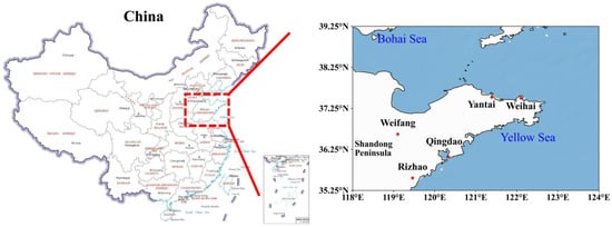
Figure 1.
Locations of five coastal cities on the Shandong Peninsula, northern China—Qingdao, Rizhao, Weifang, Weihai, and Yantai (marked with red stars in the right map). The left map highlights Shandong Province in yellow.
This study focuses on five coastal cities within Shandong Province: Qingdao, Rizhao, Weifang, Weihai, and Yantai (as depicted in Figure 1). Situated along the Shandong Peninsula, these cities serve as the peninsula’s economic hubs, replete with numerous production enterprises and extensive transport infrastructures, which contribute to significant emissions of SO2 and other pollutants. Furthermore, the meteorological conditions of coastal regions, characterized by the diurnal sea and land breezes, facilitate the dispersion and dilution of atmospheric pollutants.
2.2. Data Source and Processing
The data used in this study were divided into two main categories: predictor data and predicted SO2 concentrations. The predictor data encompassed air quality metrics and meteorological variables. Historical air quality data were sourced from the China Air Quality Online Monitoring and Analysis Platform (https://www.aqistudy.cn/, accessed on 10 April 2024), including six key atmospheric parameters (SO2, NO2, O3, CO, PM2.5, PM10) and the Air Quality Index (AQI). Meteorological parameters, including air temperature (Temp), air pressure (AirP), relative humidity (RH), wind speed (WS), and wind direction (WD), were sourced from the China Terrestrial International Exchange Station Climatological Information Daily Value Dataset (V3.0) provided by the China Meteorological Data Service Center (CMDC) (https://data.cma.cn/, accessed on 10 April 2024). The data have a daily temporal resolution spanning from 1 January 2014 to 20 September 2020. To ensure a rigorous validation process, a strict temporal segregation was applied between the training and test sets. The training set comprises the first 75% of the dataset, covering 1 January 2014 to 14 January 2019, while the test set includes the remaining 25%, extending from 15 January 2019 to 20 September 2020. This strict separation ensures that no test data were seen during training, preserving the integrity and reliability of the model evaluation.
The datasets used in this study underwent rigorous quality control to ensure reliability before analysis. Air quality and meteorological data were time-synchronized at each monitoring station by indexing pollutant concentrations with corresponding meteorological records. To maintain consistency between dependent and independent variables, all input features were normalized to the [0,1] range, which improves model stability and convergence.
Regarding data completeness, we conducted a thorough assessment and found that the majority of the meteorological dataset was fully recorded. For rare instances of missing values, we employed linear interpolation to fill minor gaps, ensuring temporal continuity without introducing significant bias. Additionally, we screened for outliers using statistical thresholds and removed extreme values likely caused by sensor errors or anomalies. These preprocessing steps ensured high data integrity and alignment, supporting robust model training and evaluation.
Here, we illustrate a significant decline in SO2 concentrations in Qingdao City from 2014 to 2020 (Figure 2a). Comparable trends were observed in the other four cities, although they are not depicted in this figure. The histogram distribution of SO2 concentrations, as depicted in Figure 2b, exhibited an off-peak pattern. To stabilize variance and enhance model performance, we applied a log transformation to SO2 concentrations. This choice was guided by the strong right-skewness of the raw SO2 data, making log transformation a natural approach for reducing heteroscedasticity and improving normality [32]. In addition, compared to the Box–Cox transformation, the log transformation provides similar effectiveness while being computationally simpler [32,33].

Figure 2.
Time series of SO2 concentrations (a), histogram distribution of SO2 concentrations (b), and logarithmically transformed SO2 concentrations (c) in Qingdao from 1 January 2014 to 20 September 2020.
Given the clear seasonal variation, with winter peaks likely driven by heating activities, we define the heating season as spanning from 15 November to 5 April of the following year, while the remainder of the year is classified as the non-heating season. For example, the 2015 heating season extends from 15 November 2014 to 5 April 2015. Notably, the 2014 heating season began on 1 January 2014, while in 2020, the non-heating season spanned from 6 April to 20 September.
3. Methods
3.1. Model Design
In this study, we developed a hybrid model that integrates the strengths of signal decomposition, feature selection, and sequence modeling to offer an accurate and robust framework for predicting short-term variations in SO2 concentrations (Figure 3). This hybrid model is referred to as RF-VMD-Seq2Seq. RF is employed to identify the most influential variables affecting SO2 concentrations as the input variables by feature selection. Given the inherent non-stationarity and multi-scale variability in SO2 time series, VMD is utilized to decompose the original signal into intrinsic mode functions (IMFs). This process captures both short-term fluctuations and long-term trends, facilitating more effective feature extraction and improving predictive accuracy. The Seq2Seq architecture, leveraging an encoder–decoder framework, is well-suited for capturing intricate temporal dependencies in air pollution data. This structure enables accurate multi-step forecasting by effectively learning complex historical patterns. The proposed framework is specifically designed to address critical challenges in SO2 forecasting, particularly within complex atmospheric environments in China.
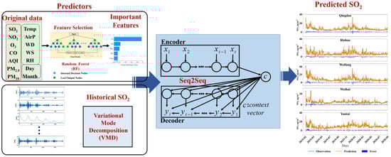
Figure 3.
Framework diagram of the RF-VMD-Seq2Seq model, integrating Random Forest (RF), Variational Mode Decomposition (VMD), and Sequence-to-Sequence (Seq2Seq) techniques.
The specific steps in the process are as follows:
Step 1: Feature Extraction. Initially, a set of 14 variables encompassing air quality indices and meteorological parameters were fed into the RF model to assess the significance of each feature. Subsequently, the established 0.05 threshold criterion was utilized to filter and retain the most influential features for subsequent analysis.
Step 2: Decomposition of SO2 Concentrations Using VMD. Recognizing the fluctuating and generally declining trend in SO2 concentrations, VMD was applied to decompose the data. This step was crucial for enhancing the model’s predictive accuracy by breaking down the complex signal into more manageable and interpretable components.
Step 3: Prediction with the Seq2Seq Model. The decomposed mode functions of logarithm-transformed SO2 concentrations are encoded by a Seq2Seq network, which then decodes the target SO2 sequence from the encoded vector. This Seq2Seq process facilitates the generation of a predictive sequence, ultimately yielding the forecasted outcomes.
In this study, we employed the Python programming language (version 3.8) for code development and data processing. The construction and training of the deep learning models were based on the TensorFlow framework (version 2.4.0). All code and models were executed in a local computing environment without the need for additional hardware acceleration devices.
3.2. Random Forest Model
To assess the impact of each input feature on the output, feature selection methods can be utilized to derive an importance score for each feature. Common techniques include RFs, decision trees, and logistic regression. In this study, the RF algorithm was employed for feature extraction, renowned for its efficiency, stability, and capacity to handle complex nonlinear relationships [34].
This study employed a standard 0.05 threshold for feature importance values (FIV), selecting features with FIV ≥ 0.05 as final inputs [35]. This statistically significant threshold ensures that only influential features contribute to the model’s predictive performance. By reducing complexity and overfitting risks, this approach enhances generalization and improves prediction accuracy on unseen data.
More importantly, the RF algorithm provides interpretability for prediction results. By analyzing FIVs within the RF model, key contributing features can be identified, offering insights into their impact on predictions. This interpretability makes RF not only a robust tool for feature selection but also a means to understand feature–outcome relationships, enhancing the transparency and reliability of the predictive process.
For RF-based feature ranking, we utilized 100 decision trees (i.e., n_estimators) with MSE as the splitting criterion. The tree depth was left unrestricted to ensure full tree growth, allowing the model to capture complex feature interactions. Feature splits were determined based on the square root of the total number of features, and bootstrap sampling was applied to enhance robustness. To ensure stability, we ran the model multiple times, consistently obtaining similar feature importance rankings. These settings and validations enhance the reliability and rigor of our feature selection process. Detailed parameters are shown in Table 1.

Table 1.
Parameter settings for Random Forest (RF), Variational Mode Decomposition (VMD), and Sequence-to-Sequence (Seq2Seq) network models.
3.3. Variational Mode Decomposition
Variational Mode Decomposition (VMD) is an advanced signal processing technique designed to effectively analyze nonlinear and non-stationary signals, making it widely applicable across various research domains. Introduced by Dragomiretskiy and Zosso [36] in 2014, VMD refines signal decomposition by iteratively extracting intrinsic mode functions (IMFs), each characterized by distinct frequency and amplitude properties. Unlike traditional EMD methods, which rely on recursive approaches prone to mode aliasing, VMD employs a fully non-recursive framework. This key innovation enhances stability, improves decomposition accuracy, and allows for independent selection of the number of modes, providing greater control over the process.
By iteratively solving a variational optimization problem, VMD adaptively determines the center frequency and bandwidth of each IMF component. This adaptive decomposition effectively separates overlapping frequency components and mitigates endpoint effects—common limitations of conventional methods such as EMD. Moreover, VMD eliminates the need for manually selecting basis functions, enabling automatic extraction of local signal features. These advantages make VMD a powerful tool for feature extraction and signal analysis in complex environmental and engineering applications.
The core principle of VMD is to decompose the original signal f(t) into k IMF components, each constrained within a limited bandwidth. This decomposition enables the extraction of frequency-domain characteristics, facilitating a more precise analysis of the signal’s spectral content. The constrained variational formulation of VMD is expressed as follows (Equation (1)):
where k represents the number of decomposition modes, represents k-th IMF weight, is the center frequency of each component, represents the Dirichlet function, and will be defined as the partial derivative for time t.
In addition, the Alternate Direction Method of Multipliers (ADMM) based on dual decomposition and the Lagrange method is used to solve Equation (2), and the alternate iterative optimization of , , and is carried out.
where represents Lagrange multiplier; represents the penalty factor, used to reduce the interference of Gaussian noise; and the setting in this paper is 2000. By introducing the Lagrange multiplier λ, the constrained variational problem is transformed into an unconstrained variational problem, and the expression of the augmented Lagrange matrix is obtained (Equation (3)).
where , , , and are the Fourier transforms of , , , and , respectively. When the convergence condition in Equation (4) is satisfied, the sequence of output modes and the corresponding center frequency can be obtained.
When applying VMD for signal decomposition, two key parameters—the number of decomposed modal functions (k) and the Lagrange multiplier update step (τ)—significantly influence its performance. If k is set too high, the extracted modes may exhibit frequency clustering or overlap, leading to redundant or indistinguishable components [36]. Conversely, an excessively low k may cause important patterns to merge into neighboring modes or be discarded, resulting in an incomplete signal representation. The update step τ also plays a crucial role, as different values lead to varying degrees of residual error, directly affecting prediction accuracy. To optimize the decomposition process, two primary approaches have been proposed: one determines k by analyzing central frequencies, while the other optimizes τ by minimizing the residual error index (REI, Equation (5)) [37]. These methods enhance the accuracy and effectiveness of VMD in capturing essential signal features.
First, we determined the optimal k value by analyzing the frequency distribution of decomposition patterns across different k values. The optimal k is identified when frequency distributions begin to cluster or overlap, indicating a balance between resolution and uniqueness in the decomposition model. Additionally, for each coastal city, the initial number of IMF components (i.e., parameter k) is selected based on spectral analysis. The final optimal k value (Table 1) is further verified by comparing model performance at k + 1 and k − 1. To comprehensively illustrate the k selection process, Table S1 presents a detailed comparison of performance indicators for k = 7, 8, 9 and 10, supporting the rationale behind the chosen k value.
Next, the Lagrange multiplier update step τ is optimized based on the REI (Table 1). Since minimizing the REI of the original sequence is crucial for ensuring high prediction accuracy, optimizing τ is a necessary step before the decomposition process.
3.4. Sequence-to-Sequence Prediction Model
3.4.1. Sequence-to-Sequence Model Design
The Seq2Seq model, initially introduced to address sequence-to-sequence challenges, operates on an encoder–decoder framework, as outlined by Sutskever et al. [24]. The role of the encoder is to transform the input sequence into a concise vector representation, and the decoder then utilizes this vector to produce the corresponding output sequence. This approach ensures that our Seq2Seq model is well-equipped to handle complex sequence prediction tasks in the domain of air pollution research, where sequence lengths may vary significantly.
In this study, we utilized a Seq2Seq model to efficiently manage variable-length sequence prediction tasks on SO2 (Figure 3). In our model, the encoder component utilizes an LSTM network to process and encode the input sequence, and the decoder similarly employs an LSTM network. The decoder begins by initializing its hidden state with the final hidden state generated by the encoder, and it sequentially generates the output sequence, making predictions based on the learned representations. The Seq2Seq model has been successfully utilized in our previous study for predicting NO2 concentrations [21].
3.4.2. Hyperparameter Tuning
In deep learning, optimizing model performance requires careful hyperparameter tuning. For the Seq2Seq model, initial hyperparameters were set based on prior experience and refined through a combination of trial-and-error and grid search. To ensure optimal performance, validation splits and multiple trials were applied to assess model convergence and generalization. Specifically, we tested LSTM units in the range of {32, 64, 128} and dropout rates between {0.2, 0.5}. The final configuration was selected after extensive experimentation. To enhance reproducibility, random seeds were set before training. The learning rate, a crucial parameter, was manually initialized and dynamically adjusted using an adaptive optimization algorithm. Additionally, an early stopping mechanism was implemented to prevent overfitting and improve generalization.
The parameter settings for the Seq2Seq model used in this study are outlined in Table 1. This configuration demonstrates the model’s structure, where the encoder and decoder layers work together to capture both temporal dependencies and make accurate predictions for variable-length sequences. A key feature of the LSTM’s gating mechanism is its ability to perform adaptive encoding and decoding, which allows the model to handle input and output sequences of different lengths. This flexibility is particularly advantageous when used in conjunction with the Seq2Seq architecture, as it removes the constraint of requiring fixed-length sequences, enabling the model to handle variable-length sequence data efficiently. For training, we used a learning rate of 0.001, and the Adam optimizer was chosen to ensure efficient convergence.
3.5. Evaluation Metrics of Model Performance
To evaluate the performance of the model, this paper used the coefficient of determination (R2), Pearson’s correlation coefficient (Pearson’s r), root mean square error (RMSE), mean absolute error (MAE), and mean absolute percentage error (MAPE). The formulas for these evaluation indices are as follows:
where is the value of the observed data; is the predicted data; and and are the average of the observed and predicted data, respectively.
4. Results and Discussion
4.1. Long-Term Trend of SO2 from VMD
The long-term trend of SO2 levels from 2014 to 2020 was assessed through decomposing the original data by the VMD method (Figure 4). A significant decreasing trend (p < 0.0001) was observed across all five cities, based on the IMF1 component of the decomposition results (Figure 4). Weihai and Yantai show a milder decline in SO2 concentrations, with slopes exceeding −0.01, while the other three cities exhibit a more pronounced long-term decrease (slopes below −0.01), particularly Weifang, where the slope reaches −0.023. These variations in long-term trends align with the relative amplitudes of SO2 concentrations across the cities: SO2 levels are lowest in Weihai and Yantai (under 60 μg/m3), followed by Qingdao and Rizhao (peaking around 70 μg/m3), with the highest levels observed in Weifang (above 120 μg/m3). A similar downward trend in SO2 concentrations in Qingdao was observed by Meng et al. [30]. Additionally, Zhang et al. [38] reported that the mean planetary boundary layer SO2 vertical column densities exhibited a decreasing trend after 2007, followed by a rebound around 2011, and subsequently a continuous decline from 2011 to 2020 in Qingdao, Rizhao, and Yantai. Given that over 90% of China’s SO2 emissions stem from the combustion of coal, oil, and other fuels [39], this trend suggests that Shandong Province has made significant progress in reducing air pollution through the implementation of emission control policies.
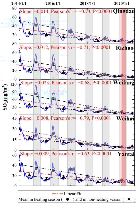
Figure 4.
Long-term trends in SO2 from 1 January 2014, to 20 September 2020, based on the IMF1 component of VMD decomposition in five coastal cities of northern China (Qingdao, Rizhao, Weifang, Weihai, and Yantai). Blue lines indicate SO2 concentrations, with black solid dots representing mean SO2 levels during heating seasons and black solid triangles indicating mean SO2 levels in non-heating seasons. The red dot-dash lines show the linear fit for all SO2 concentrations, while the black dot-dash lines show the linear fits for SO2 concentrations during heating and non-heating seasons separately. The gray shadings represent heating seasons, while the red shading marks the COVID-19 period.
In addition, the significant decline in SO2 concentrations during the heating seasons occurred more rapidly than during the non-heating seasons across the five coastal cities (Figure 4, black dash-dotted lines), which constitutes the primary contribution to the overall decrease in SO2 levels. Shandong Province has implemented the CAAP since 2013, which promotes replacing coal with gas for heating and using gas instead of oil for transportation. In December 2017, the ‘Plan for Clean Heating in Winter in Northern China (2017–2021)’ was introduced to further reduce reliance on traditional coal heating. These measures likely contributed to the overall downward trend in SO2 levels from 2014 to 2020, with a marked decrease during the 2018 heating season. Meng et al. [30] also confirmed the impact of the ‘Coal-to-Natural Gas’ policy on the SO2 decreasing trend in Qingdao from 2013 to 2019 using the closed interval of the deweathered percentage change method.
The decomposition analysis of logarithm-transformed SO2 concentrations across five coastal cities from 2014 to 2020 is presented in Figure 5, along with the corresponding frequency spectrum derived from Hilbert transform. The parameters, including the number of modes k and the optimized τ, are determined for VMD through the minimization of REI (Table 1). However, it remains challenging to determine the optimal number of components into which the original series should be decomposed [40]. Decomposing the series into too few components may fail to capture important features in the raw data, while using too many components can increase computational costs during model training. Through experimentation, we observed that the optimal number of decomposition modes can be identified by the distinct aliasing phenomenon of the center frequency in the last component. For instance, in Weihai City, this study found that when k = 10, the frequency spectrum of the 10th mode exhibited noticeable aliasing (Figure 5(d2)). Upon comparison with the prediction results for k = 9, the model performed better with 10 components, which was ultimately selected as the optimal number. These optimal parameters help ensure that the VMD decomposition is both precise and effective, providing accurate representation and enhancing the performance of subsequent analyses or predictions.
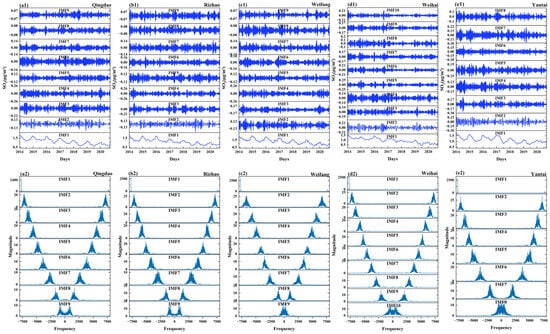
Figure 5.
Intrinsic mode functions (IMFs) extracted via Variational Mode Decomposition (VMD) (a1–e1), along with the frequency spectrum derived from the Hilbert transform (a2–e2), for five coastal cities: Qingdao (a1,a2), Rizhao (b1,b2), Weifang (c1,c2), Weihai (d1,d2), and Yantai (e1,e2).
By decomposing complex signals into IMF of different frequencies, VMD effectively separates long-term trends from short-term fluctuations (Figure 5). A low-frequency IMF, such as IMF1, is critical to capturing downtrends because it reflects longer-term changes related to macro factors such as policy adjustments. Ignoring the low-frequency IMF will cause the model to fail to identify the downward trend, making the analysis results incomplete. The high-frequency IMF focuses on dealing with short-term fluctuations such as daily/weekly fluctuations, which are often related to short-term factors such as meteorological events. High-frequency IMF can isolate these short-term changes and provide a clear signal for analysis. Without the high-frequency IMF, the model would not be able to capture short-term fluctuations, affecting the understanding of the overall characteristics of the data. The frequency ranges of the IMF components for each site are detailed in Table S2.
4.2. Weekly Cycle as the Input Sequence-Length from VMD
The choice of input sequence-length directly affects the performance of deep learning model [41,42]. A too short time step may result in the model failing to capture the input features fully, while a too long-time step may lead to overfitting. To determine the most effective input sequence length for short-term SO2 forecasting, we examined the frequency bands and Variance Accounted For (VAF) across five coastal cities, excluding the low-frequency band in IMF1 (Figure 5). In contrast, the sub-seasonal periodicities observed in IMF2 (12–20 days) likely correspond to mesoscale atmospheric and oceanographic processes, including local wind systems, ocean currents, upwelling zones, and sub-seasonal oscillations (e.g., the Madden-–Julian Oscillation and variations in the East Asian Monsoon) [32,43,44]. Additionally, anthropogenic influences, such as fluctuations in industrial emissions and regional transport of pollutants, may contribute to variations at this timescale. These medium-scale periodicities provide deeper insights into pollutant transport mechanisms, extending beyond daily meteorological fluctuations and enhancing the understanding of multi-scale air pollution dynamics.
Table 2 shows that SO2 in IMF3–IMF10 exhibits periodicities between 2 and 11 days, while IMF2 contains frequencies corresponding to periods ranging from 12 to 20 days.
Table 2.
Identified periodicities using the Variational Mode Decomposition (VMD) method and corresponding Variance Accounted For (VAF) across five coastal cities.
The high-frequency bands (IMF3–IMF10) align with the synoptic mode of variability (SMV), which governs atmospheric fluctuations on similar timescales [32,42,45]. SMV is influenced by a combination of remote atmospheric teleconnections, sub-seasonal patterns such as atmospheric waves, regional circulations, and local weather responses to synoptic state perturbations [46]. The high-frequency modes are essential for short-term forecasting and understanding the temporal variability [47]. Furthermore, the high-frequency IMFs can be linked to well-known short-term meteorological and human activity patterns. For example, in coastal regions, the diurnal cycle of sea breezes can induce recurrent variations in pollutant dispersion, while weekly traffic cycles contribute to regular short-term fluctuations in emissions [48]. These practical phenomena help explain the observed 2–11 days periodicities, underscoring the relevance of our time-series decomposition in capturing dynamic and transient features of air pollution.
In contrast, the sub-seasonal periodicities observed in IMF2 (12–20 days) likely correspond to mesoscale atmospheric and oceanographic processes, including local wind systems, ocean currents, upwelling zones, and sub-seasonal oscillations (e.g., the Madden–Julian Oscillation and variations in the East Asian Monsoon) [32,43,44]. Additionally, anthropogenic influences, such as fluctuations in industrial emissions and regional transport of pollutants, may contribute to variations at this timescale. These medium-scale periodicities provide deeper insights into pollutant transport mechanisms, extending beyond daily meteorological fluctuations and enhancing the understanding of multi-scale air pollution dynamics.
Table 2 also shows that the high-frequency bands, with periods ranging from 2 to 11 days, account for 18.4% to 33.8% of the total variance in daily SO2 measurements, while IMF2 periodicities (12–19 days) explain 4.6% to 7.4% of the variance. Based on these findings, we designed six training experiments with input sequence lengths of 1, 3, 5, 6, 7, and 15 days. The results revealed that an input sequence length of 7 days demonstrated good performance for SO2 predictions, with lower errors (RMSE and MAE) and higher correlations (Pearson’s r and R2) in Weifang, Weihai, and Yantai (Figure 6). In Qingdao and Rizhao, a 15-day input sequence length provided slightly better prediction performance than 7 days, which still outperformed other input lengths (Figure 6). These findings suggest that the weekly-cycle variations predominantly influence the accuracy of one-day-ahead SO2 predictions across the coastal regions of Shandong Peninsula, particularly in the northern part (Weifang, Weihai, and Yantai), while the biweekly scale variations play an equally or even more significant role in prediction accuracy in the southern regions, such as Qingdao and Rizhao. To maintain model consistency and ensure generalization, we selected a 7-day input sequence length for this study.
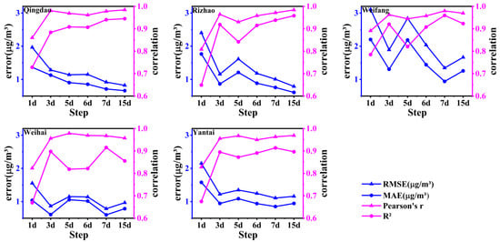
Figure 6.
Statistical estimation of different historical time steps used as input sequence lengths for the test sets across five coastal cities. The blue lines represent the root mean square error (RMSE) and mean absolute error (MAE), while the pink lines indicate the correlation coefficients (Pearson’s r and R2).
Research has shown that SO2 and other air pollutants exhibit notable weekly cycles, with higher concentrations observed on weekdays compared to weekends [49,50]. Weekly cycles provide a valuable framework for distinguishing anthropogenic influences from natural causes, as only human activities are likely to drive variations in concentrations, temperatures, or other atmospheric variables on a seven-day cycle [50,51]. Our study employed data from the past 7 days to predict SO2 concentrations for the next day, effectively considering the ‘weekend effect’ and highlighting the anthropogenic sources of SO2 in northern China’s coastal cities.
4.3. Influence of Anthropogenic Emission on SO2 Prediction by RF
Figure 7 illustrates the FIVs obtained through RF feature extraction across five coastal cities. For each city, features with FIVs exceeding 0.05 were selected as input variables, resulting in total FIVs ranging from 0.74 to 0.79. Among the selected predictors, CO and RH are common across all five cities, while air temperature is included in four cities, excluding Rizhao. Furthermore, NO2 and PM10 are identified as significant predictors in three cities.
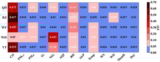
Figure 7.
Feature importance values (FIVs) calculated by Random Forest (RF) model for 5 coastal cities (Qingdao, QD; Rizhao, RZ; Weifang, WF; Weihai, WH; and Yantai, YT), and important features with FIVs over 0.05 as input variables.
Compared to meteorological variables, air pollutants such as CO, NO2, and PM10 have a more pronounced impact on SO2 prediction, accounting for over 60% of the variation in SO2 (Figure 7). Previous studies have shown that the gaseous pollutants CO and NO2 share common anthropogenic emission sources with SO2 [52,53]. This relationship makes their concentration changes highly relevant for predicting SO2 levels in our model, contributing over 50% to the model’s accuracy (Figure 7).
Additionally, the primary sources of particulate matter, such as PM10 and PM2.5, include industrial emissions, traffic exhaust, biomass burning, coal combustion, and other human activities [54,55,56]. As SO2 is a gaseous pollutant that can chemically react with other gases and particulate matter, it contributes to the formation of sulfate and related compounds [57,58,59,60]. These reactions help form particulate matter, underscoring a strong connection between particulate matter concentrations and SO2 levels. Therefore, our findings suggest that emissions from anthropogenic activities are shared contributors to both particulate matter and SO2 concentrations.
In addition, meteorological conditions, RH and Temp, have an important influence on the model’s prediction accuracy (Figure 7). This is due to the influence of RH and Temp on chemical reaction rates and the processes of diffusion and dilution in the atmosphere [57,60]. Specifically, increases in RH and Temp accelerate chemical reaction rates, leading to higher SO2 production. Furthermore, elevated RH and temperatures promote faster diffusion and dilution of SO2 in the atmosphere.
4.4. SO2 Predicting Performance
In this section, the effectiveness of the RF-VMD-Seq2Seq model in predicting SO2 concentration is experimentally analyzed in the test set. First, the most relevant input variables for each coastal city were selected from a total of 11 variables after applying the RF method, with the sum of FIVs greater than 0.74 (Table 3). This targeted selection process refines the input set, enhancing the overall accuracy and robustness of the RF-VMD-Seq2Seq model by focusing on the most significant variables affecting predicted concentrations.
Table 3.
Important features selected by Random Forest (RF) as input predictors across five coastal cities in the RF-VMD-Seq2Seq model.
After evaluating the model performance on the training set, we applied the RF-VMD-Seq2Seq model to a test set. Figure 8 presents a time series comparison of predicted SO2 concentrations versus observed concentrations for five coastal cities over the test set period (15 January–20 September 2020). The predicted SO2 concentrations from the test set closely match the observed values in each city, with most differences remaining within 1 µg/m3. Additionally, there was a slight overestimation in predicting the lower concentrations of SO2 in Qingdao and Weihai, yet the RF-VMD-Seq2Seq model still performed well overall, as shown in Figure 8. Despite these minor discrepancies, the model demonstrated strong predictive accuracy and effectively captured key trends in SO2 concentrations across the coastal cities.
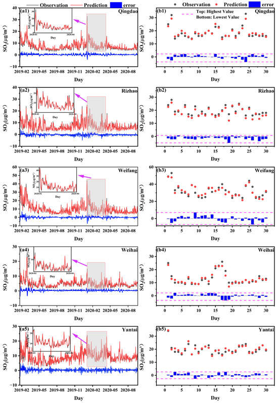
Figure 8.
Comparison of time-series SO2 concentrations predicted by the RF-VMD-Seq2Seq model with observed values across five coastal cities: Qingdao, Rizhao, Weifang, Weihai, and Yantai. Panels (a1–a5) show the complete time series within the test dataset, while panels (b1–b5) highlight the upper 5% of SO2 concentrations. The red lines represent predicted values, black lines denote observed values, and blue lines illustrate the differences between predictions and observations. The gray-shaded regions indicate the COVID-19 lockdown period in 2020.
However, when analyzing the differences in model performance, we found that the geographical, climatic, and industrial characteristics of different cities have a significant impact on the predicted results. For example, Weifang, as an important industrial town, has concentrated heavy industry activities and large pollutant emissions. Moreover, its continental monsoon climate (hot and rainy in summer and cold and dry in winter) tends to exacerbate pollutant accumulation, thus affecting the model prediction performance. In contrast, Weihai has little industrial activity and pays attention to ecological protection, and its maritime climate (mild, small temperature difference between day and night) facilitates the diffusion of pollutants. In addition, Weihai is a tourist city, and seasonal population movements may cause short-term fluctuations in pollutant emissions and model predictions.
The RF-VMD-Seq2Seq model demonstrates exceptional performance in capturing both fluctuations and outliers in SO2 concentrations, including extreme events such as the sharp declines observed during the Spring Festival and the COVID-19 pandemic in 2020 (Figure 8(a1–a5), gray areas and subplots). Detailed metrics are shown in Table S4. Notably, SO2 concentrations peaked each year during the Spring Festival from 2014 to 2019, then quickly returned to high levels after the holiday. However, from late January to March 2020 (see red rectangle in Figure 4), this transition became more prolonged and pronounced due to the combined effects of the Spring Festival and the progressive lockdown measures implemented during the COVID-19 pandemic in China [61]. The pandemic, particularly in early 2020, led to a significant reduction in industrial and transportation emissions, introducing irregularities in the data. This resulted in a sharp drop in SO2 concentrations, temporarily deviating from historical seasonal trends. While our model effectively captured the overall downward trend, the abrupt emission reductions and the subsequent gradual recovery posed challenges for short-term forecasting accuracy.
Moreover, the model effectively handles the upper 5% of SO2 concentrations (mostly exceeding 10 μg/m3), with predicted values closely matching observed measurements, demonstrating its robustness in capturing extreme pollution events (Figure 8(b1–b5)). This ability to predict extreme values is critical, as prior studies have established that elevated SO2 levels—such as a 10 μg/m3 increase in daily concentrations—are associated with adverse health outcomes, including hypertension, all-cause mortality, and respiratory mortality [62,63,64,65].
The majority of the top 5% of SO2 concentrations occur between December and March, coinciding with the heating season. Increased heating demand leads to higher coal consumption, making it a major source of SO2 emissions, particularly in northern cities where winter concentrations are significantly higher than in non-heating periods [48,59]. Additionally, extreme pollution events contribute to high SO2 levels, often driven by adverse meteorological conditions such as dense fog, low wind speeds, temperature inversions, and air flow convergence. These factors collectively hinder pollutant dispersion, leading to localized SO2 accumulation [60].
Accurate prediction of SO2 levels is vital for mitigating public health risks, particularly during unusual events that disrupt normal pollution patterns. The RF-VMD-Seq2Seq model’s integration of variational mode decomposition ensures the detection and analysis of non-stationary trends, while its sequence-to-sequence framework enables the capture of complex temporal dynamics. By effectively addressing both routine fluctuations and extreme variations, this model confirms its capability to provide reliable forecasts, supporting air quality management and health protection efforts.
The density scatter plots of the predicted vs. observed SO2 concentrations in five coastal cities are illustrated in Figure 9. Most of the data points are close to the bisector (black dashed lines in Figure 9), indicating a high level of agreement between predicted and observed values, especially in Weifang City. Under lower SO2 pollution conditions (less than 10 µg/m3), there is a slight overestimation in Qingdao and Weihai, while for higher pollution levels, there is a slight underestimation. In Yantai, the model shows a slight overall overestimation.
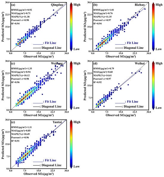
Figure 9.
Density scatter plots of the predicted vs. observed SO2 concentrations in the test set, along with statistical evaluation metrics, for (a) Qingdao, (b) Rizhao, (c) Weifang, (d) Weihai, and (e) Yantai.
The variation in model performance across cities likely stems from differences in local meteorological conditions and emission characteristics. For example, Weifang, an industrial hub with significant petrochemical and manufacturing activities, has higher SO2 emissions due to industrial combustion (Figure 8). In contrast, the other four cities, which are coastal and driven by tourism with relatively lower industrial emissions, exhibit different pollution dynamics. Additionally, Weifang’s inland location (Figure 1) results in weaker coastal wind influence, whereas strong marine airflows in coastal cities enhance pollutant dispersion [48]. This increased variability contributes to more complex pollution fluctuations, slightly reducing model accuracy in these regions.
Statistically, lower errors and higher correlations further support the strong predictive capability of the RF-VMD-Seq2Seq model across five coastal cities (Figure 9). The RMSE values, ranging between 0.79 μg/m3 and 1.35 μg/m3, along with the MAE values from 0.60 μg/m3 to 0.85 μg/m3 and MAPE values between 10% and 15%, reflect minimal fluctuations and differences between predicted and observed SO2 concentrations.
Moreover, Pearson’s r coefficient greater than 0.96 indicates a strong linear relationship between predictions and actual values. Overall, the RF-VMD-Seq2Seq model demonstrates excellent predictive performance with high accuracy on SO2. This is further supported by an R2 value above 0.91, confirming that the input variables used in the model effectively explain most of the data variation. Overall, these results demonstrate the RF-VMD-Seq2Seq model accurately captures SO2 concentrations even under varying pollution conditions, showing its robustness in handling both lower and higher pollution levels.
4.5. The Role of VMD in Predicting Downward Trend of SO2
To more comprehensively assess the role of VMD in enhancing the performance of the RF-VMD-Seq2Seq model for predicting SO2 concentrations in coastal cities of northern China, we conducted a detailed comparison with the RF-Seq2Seq model using EEMD decomposition (RF-EEMD-Seq2Seq) and the RF-Seq2Seq model without decomposition. To ensure a fair, apple-to-apple comparison, all models were trained and tested on the same samples, allowing for a consistent evaluation of their predictive accuracy and robustness.
Figure 10 shows the comparison of RF-VMD-Seq2Seq with RF-EEMD-Seq2Seq and RF-Seq2Seq. The RF-Seq2Seq model performed the worst across all five cities, with errors (RMSE, MAE, and MAPE) increasing by 113% to 496% and correlations decreasing by 33% to 99%, compared to the other two models (detailed metrics are shown in Table S3). When comparing the RF-EEMD-Seq2Seq model with RF-VMD-Seq2Seq model, we observed a decline in performance in terms of Pearson’s r and R2, with a reduction ranging from 6% to 10% and from 13% to 40%, respectively. The high accuracy of this method is attributed to the use of the VMD algorithm, which successfully decomposes the original SO2 concentration sequence into multiple independent components. This decomposition strategy allows each component to be predicted independently, greatly simplifying the complexity of the prediction task.
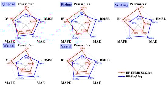
Figure 10.
Comparison of the proportional change in statistical indicators for the RF-EEMD-Seq2Seq and RF-Seq2Seq models relative to the RF-VMD-Seq2Seq model across five coastal cities. The red lines represent the proportional changes for RF-EEMD-Seq2Seq, while the blue lines denote those for RF-Seq2Seq.
In detail, the time series of predicted results from RF-EEMD-Seq2Seq and RF-Seq2Seq are shown in Figure 11. Without data decomposition in the prediction process, the RF-Seq2Seq model failed to capture the variation in SO2 levels, particularly its trend (Figure 11). This highlights that the use of signal decomposition methods, such as VMD and EEMD, significantly improves prediction accuracy for downward SO2 concentrations.
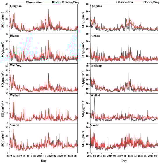
Figure 11.
Time-series comparison of observed SO2 concentrations with predictions in the test set using the RF-EEMD-Seq2Seq model (left panel) and the RF-Seq2Seq model (right panel). The red lines represent the predicted values, while the black lines denote the observed values.
Regarding the comparison of RF-Seq2Seq models integrated with EEMD and VMD, although RF-EEMD-Seq2Seq effectively captured the overall trend of SO2 concentrations, it struggled with extreme values. Specifically, it exhibited overestimations during periods of heavy pollution in February 2019 across five coastal cities (Figure 11). Conversely, during the 2020 Spring Festival, the model underestimated extreme high values in Qingdao and Weifang (Figure 11). Additionally, it consistently underestimated low SO2 concentrations in Qingdao and Rizhao (Figure 11). Decomposing non-stationary data into multiple components, each with unique frequencies, is essential for enhancing the accuracy of predictive models by providing deeper insights into underlying data patterns and trends. EMD-based models struggle with mode aliasing and end effects, lack a strong theoretical foundation, and have a more complex sifting process [66]. These factors can restrict the overall effectiveness of the hybrid prediction approach. VMD effectively mitigates mode aliasing by optimizing the variational problem, ensuring a more accurate decomposition of complex signals. Additionally, it provides flexible control over the decomposition process by allowing adjustments to the number of modes and bandwidth parameters, enabling a more precise extraction of meaningful patterns from the data [36,67,68]. Our study further indicates that the VMD decomposition method is more effective at explaining the variability in the data and may fully capture the complex and downward trends within the SO2 concentration data.
Additionally, in comparing the performance of Seq2Seq with traditional LSTM models, our findings indicated that RF-Seq2Seq models more accurately capture general trends and disruptions, regardless of whether RF-based feature selection is applied [22]. This advantage stems from the Seq2Seq architecture’s ability to effectively model complex temporal dependencies, making it particularly suited for handling the dynamic nature of air quality data. Building upon this, we further enhanced SO2 prediction accuracy in this study by integrating VMD into the RF-Seq2Seq framework. By decomposing complex signals into IMFs, VMD allows the model to extract meaningful patterns across multiple time scales, leading to more precise predictions. Our findings demonstrate that incorporating a signal decomposition step via VMD significantly refines the input data for the Seq2Seq model, ultimately improving predictive accuracy and robustness compared to traditional forecasting methods.
In addition, random seeds were set in all experiments to ensure consistent initialization conditions, thereby minimizing performance fluctuations caused by randomness. This approach guarantees repeatability and ensures that performance differences across multiple runs are due to methodological differences rather than stochastic variations. However, despite fixing random seeds, we observed variations in RF-EEMD-Seq2Seq outputs due to the inherent noise sensitivity and iterative nature of EEMD. In contrast, RF-VMD-Seq2Seq demonstrated consistently better performance across multiple trials, confirming the stability of its improvement. These findings indicate that VMD provides a more reliable decomposition framework, reinforcing the superiority of RF-VMD-Seq2Seq over RF-EEMD-Seq2Seq.
4.6. Practical Implication
4.6.1. Operational Deployment
The proposed RF-VMD-Seq2Seq model demonstrates high operational efficiency, making it suitable for real-time or near-real-time environmental monitoring applications. The model has a fast prediction time, requiring no more than 30 min per forecast, and it operates with low computational resource consumption. It runs efficiently on systems with less than 8 GB of memory, eliminating the need for specialized hardware. This allows seamless integration into existing air quality forecasting platforms without additional infrastructure costs, enhancing both applicability and flexibility.
The model requires continuous air quality monitoring data, including SO2 concentrations, meteorological variables (e.g., temperature, humidity, wind speed), and historical pollutant trends. Integration with real-time air quality monitoring networks can enable automated data ingestion and preprocessing, ensuring timely forecasting updates.
By streamlining the operational workflow and ensuring computational feasibility, this forecasting framework can serve as a practical decision-support tool for air quality management and early warning systems.
4.6.2. Limitation and Improvement Project
In this study, we employed a 75:25 ratio to partition the dataset into training and test sets. This decision was guided by the sequential nature of time series data, ensuring that data were split strictly in chronological order to prevent information leakage. Through multiple experiments, we found that this ratio provided the optimal balance between sufficient training data for model learning and a representative test set for performance evaluation. While we acknowledge potential limitations—such as the influence of time-specific events (e.g., policy changes or the COVID-19 period) and the periodicity of air pollution trends—this split remains suitable given the objectives of our study. More advanced validation techniques, such as time-series cross-validation or rolling-window methods, could further enhance robustness. However, considering computational efficiency and the stability of our results, the selected partitioning method is sufficient to support the validity of our conclusions.
Our findings indicate that anthropogenic gases such as CO and NO2 are strong predictors of SO2 concentrations, highlighting a strong synergy between their emission sources. This suggests that policies aimed at reducing CO and NO2 emissions—such as stricter controls on fossil fuel combustion in power plants, industrial processes, and vehicle emissions—could simultaneously contribute to SO2 reduction. By identifying these co-pollutants as key indicators, local policymakers can develop more integrated air quality management strategies. For instance, enhancing monitoring efforts for CO and NO2 can serve as an early warning system for SO2 pollution episodes. Moreover, multi-pollutant control policies, such as promoting cleaner industrial production and transitioning to low-emission energy sources, could yield more efficient and cost-effective improvements in air quality.
Our approach is particularly effective in regions experiencing policy-driven emission reductions, such as China’s ‘Coal-to-Gas’ transition. However, its generalizability to other countries depends on industrial structures, energy policies, and climatic conditions. In regions where coal remains a dominant energy source without similar policy interventions, the model may need adjustments to account for different emission dynamics. Nevertheless, the methodology—decomposing pollutant time series and integrating meteorological factors—can be adapted to other settings with appropriate modifications. For instance, in countries with seasonal biomass burning or stricter industrial regulations, alternative predictor variables (e.g., wildfire emissions, vehicle restrictions) may be required. Additionally, the model’s temporal resolution and data sources may need to be adjusted based on local monitoring capabilities.
As SO2 emissions continue to decline due to strengthened environmental policies and industrial transformations, the time-series patterns of air pollution may undergo significant changes. This could impact the stability and generalizability of our model. To ensure continued accuracy, periodic retraining of the RF-VMD-Seq2Seq model is necessary, especially when major policy shifts or emission reductions alter historical trends. An annual update strategy, incorporating the most recent data, could help maintain model adaptability. Additionally, implementing an adaptive learning framework that dynamically adjusts to new emission patterns and external factors would enhance long-term forecasting reliability.
The RF-VMD-Seq2Seq architecture can be extended for multi-day-ahead forecasting, but forecast accuracy tends to decline as the lead time increases (Table S5). For example, under the same framework and parameter settings, we found that when predicting 2-day and 3-day horizons, the errors approximately doubled, and by the 5-day-ahead forecast, the errors tripled compared to the 1-day-ahead prediction in Qingdao. The determination coefficients decreased from over 0.90 to below 0.60, while correlation coefficients dropped from 0.98 to 0.83. This suggests that while the model retains some predictive capability over longer horizons, the accumulation of uncertainty presents challenges. Future improvements could involve optimizing decomposition parameters, integrating additional exogenous variables, or leveraging ensemble learning techniques to enhance multi-day forecasting accuracy.
Currently, our model relies primarily on historical meteorological data for forecasting SO2 concentrations. However, integrating real-time meteorological forecasts from numerical weather prediction models could further enhance predictive accuracy, particularly for extended forecast horizons. Incorporating forecasted temperature, wind speed, humidity, and atmospheric pressure would enable the model to better anticipate pollution dispersion dynamics and potential anomalies. Future research could explore hybrid approaches that fuse historical data with real-time weather forecasts, improving the model’s applicability for proactive air quality management and decision making by city environmental bureaus.
An hourly modeling framework could be beneficial for regions experiencing rapid pollution fluctuations, such as industrial zones or areas affected by traffic congestion. Hourly forecasting would enable early warnings of short-term pollution spikes, enhancing real-time air quality management. However, transitioning to an hourly model presents several challenges. Data availability is a key concern, as high-resolution air quality and meteorological data must be consistently available with minimal gaps to ensure reliable predictions. Computational load is another factor, as hourly forecasting significantly increases data volume and model complexity, requiring enhanced computational resources. Lastly, shorter temporal dependencies must be accounted for, as hourly variations are influenced more by immediate meteorological shifts and transient emissions, necessitating more frequent updates and potentially different decomposition parameters (e.g., finer-scale IMFs). Future research could explore hybrid approaches, integrating real-time sensor data and high-resolution meteorological forecasts to refine sub-daily predictions while balancing computational efficiency.
In future research, we prioritize extending this modeling approach to PM2.5 due to its severe health impacts and complex formation mechanisms involving both primary emissions and secondary chemical reactions. Compared to SO2, PM2.5 exhibits more intricate temporal variability, influenced by meteorological conditions, precursor gases (e.g., SO2, NO2, and VOCs), and regional transport. Applying the decomposition method to PM2.5 may require more IMFs to capture both short-term fluctuations and long-term seasonal trends. Additionally, different periodic cycles—such as weekly human activity patterns and synoptic-scale meteorological shifts—would need to be considered.
5. Conclusions
In this study, the RF-VMD-Seq2Seq model was established based on random forest feature selection, VMD, and Seq2Seq methods to predict SO2 concentration in five cities in the Shandong Peninsula. The results are as follows:
The RF-VMD-Seq2Seq model demonstrates strong performance in predicting SO2 concentrations across the five coastal cities in Shandong Province, with R2 values exceeding 0.91 at nearly all sites. The Pearson’s r was generally above 0.96, while RMSE remained below 1.35 μg/m3, MAE stayed below 0.94 μg/m3, and MAPE consistently remained below 15%. The VMD decomposition method outperformed the EEMD method in capturing the variability in the data, effectively addressing the complex and non-linear trends in SO2 concentration. Without decomposition, prediction accuracy significantly decreased, with errors doubling and correlations dropping by 33–99%. VMD decomposition significantly improves the predictive performance of standard Seq2Seq. The average indexes in Qingdao, Rizhao, Weifang, Weihai, and Yantai were improved as follows: RMSE decreased by 2.78 μg/m3, MAE decreased by 1.78 μg/m3, MAPE decreased by 23.65, R2 increased by 0.73, and Pearson’s r increased by 0.40.
A significant decreasing trend in SO2 concentrations was observed across all five cities based on VMD decomposition. Notably, the decline in SO2 concentrations during the heating seasons occurred more rapidly than during the non-heating seasons across the five coastal cities. The high-frequency bands from VMD decomposition serve as effective references for determining the input sequence length of the RF-VMD-Seq2Seq model. A 7-day input sequence length enables accurate prediction for the following day, effectively capturing the ‘weekend effect’ and emphasizing the influence of anthropogenic sources of SO2 in the coastal cities of northern China.
The dataset was processed using an RF algorithm to calculate importance scores for each input feature, allowing the selection of key features that reflect how the Seq2Seq model interprets the predictors. Overall, gaseous pollutants had a greater influence on SO2 prediction compared to meteorological factors. CO, NO2, and PM10 had a more pronounced impact on SO2 prediction, accounting for over 60% of the variation in SO2. For the meteorological factors, RH and temperature played critical roles due to their influence on atmospheric chemical reactions, wet deposition, and dilution processes.
Although the RF-VMD-Seq2Seq model proposed in this study delivers strong results for one-day-ahead SO2 prediction, its application is currently limited to short-term forecasting. A potential direction for future improvement is the development of a more integrated model that can predict air pollutants over the medium and long term, achieving even better performance.
Supplementary Materials
The following supporting information can be downloaded at https://www.mdpi.com/article/10.3390/su17062546/s1. Table S1. Comparison of model performance metrics across different mode k values (k = 7, 8, 9, 10) in VMD. The bold fonts highlight the decomposition results under the optimal mode; Table S2. The central frequency of the intrinsic mode function (IMF) across five coastal cities; Table S3. Performance comparison of different forecasting methods: RF-VMD-Seq2Seq, RF-EEMD-Seq2Seq, and RF-Seq2Seq; Table S4. Model performance indicators for predicting SO2 concentration during COVID-19 across five coastal cities; Table S5. Model performance of different input-sequence length used for Forecasting in RF-VMD-Seq2Seq.
Author Contributions
Conceptualization, X.G.; Methodology, R.Z., Y.G. and R.W.; Software, G.W., X.L., Y.G. and R.W.; Validation, G.W., R.Z., X.G. and X.L.; Formal analysis, R.Z., X.G., Y.G., W.Y., H.L. and T.Z.; Investigation, G.W., R.Z., X.G., X.L. and W.Y.; Resources, X.G. and H.G.; Data curation, G.W.; Writing—original draft, G.W.; Writing—review & editing, R.Z., X.G., W.Y., R.W., H.L. and T.Z.; Supervision, H.G.; Project administration, T.Z.; Funding acquisition, H.L. and H.G. All authors have read and agreed to the published version of the manuscript.
Funding
This work was supported by the National Nature Science Foundation of China-Shandong Joint Fund (U1906215) and the Key Laboratory of Mathematics and Engineering Applications, Ministry of Education. This work was also funded by the Science and Technology Development Strategy Research Project of the Ministry of Natural Resources of China (2023-ZL-72) and Jinan Science and Technology Bureau (202228034). The authors are very grateful to Xingbin Jia for his helpful advice and to the anonymous referees for their useful comments.
Institutional Review Board Statement
Not applicable.
Informed Consent Statement
Not applicable.
Data Availability Statement
The raw data supporting the conclusions of this article will be made available by the authors on request.
Conflicts of Interest
The authors declare no conflict of interest.
Abbreviations
| Abbreviations | Full Forms |
| ADMM | Alternate Direction Method of Multipliers |
| AirP | Air Pressure |
| ANN | Artificial Neural Network |
| AQI | Air Quality Index |
| ARIMA | Autoregressive Integrated Moving Average |
| ARMA | Auto-Regressive Moving Average model |
| BiLSTM | Bidirectional Long Short-Term Memory |
| BSPC | Blue Sky Protection Campaign |
| CAAP | Clean Air Action Plan |
| CMAQ | Community Multi-Scale Air Quality |
| CNN | Convolutional Neural Networks |
| COVID-19 | Novel Coronavirus Pneumonia |
| EEMD | Ensemble Empirical Mode Decomposition |
| EMD | Empirical Mode Decomposition |
| FIVs | Feature importance values |
| GAT | Graph Attention Networks |
| GC-LSTM | Graph Convolutional networks and LSTM |
| IMFs | Intrinsic Mode Functions |
| LSTM | Long Short-Term Memory |
| MAE | mean absolute error |
| MAPE | mean absolute percentage error |
| MLR | Multiple Linear Regression |
| Pearson’s r | Pearson’s correlation coefficient |
| R2 | Coefficient of Determination |
| REI | Residual Error Index |
| RF | Random Forest |
| RH | Relative Humidity |
| RMSE | root mean square error |
| RNNs | Recurrent Neural Networks |
| Seq2Seq | Sequence-to-Sequence |
| SMV | Synoptic Mode of Variability |
| SO2 | Sulfur Dioxide |
| Temp | air temperature |
| VAF | Variance Accounted For |
| VMD | Variational Mode Decomposition |
| WD | Wind Direction |
| WS | Wind Speed |
References
- Zhu, S.; Wang, X.; Mei, D.; Wei, L.; Lu, M. CEEMD-MR-Hybrid Model Based on Sample Entropy and Random Forest for SO2 Prediction. Atmos. Pollut. Res. 2022, 13, 101358. [Google Scholar] [CrossRef]
- Van Der A, R.J.; Mijling, B.; Ding, J.; Koukouli, M.E.; Liu, F.; Li, Q.; Mao, H.; Theys, N. Cleaning up the Air: Effectiveness of Air Quality Policy for SO2 and NOx Emissions in China. Atmospheric Chem. Phys. 2017, 17, 1775–1789. [Google Scholar] [CrossRef]
- Wang, T.; Wang, P.; Theys, N.; Tong, D.; Hendrick, F.; Zhang, Q.; Van Roozendael, M. Spatial and Temporal Changes in SO2 Regimes over China in the Recent Decade and the Driving Mechanism. Atmos. Chem. Phys. 2018, 18, 18063–18078. [Google Scholar] [CrossRef]
- Zhang, H.; Wang, Y.; Hu, J.; Ying, Q.; Hu, X.-M. Relationships between Meteorological Parameters and Criteria Air Pollutants in Three Megacities in China. Environ. Res. 2015, 140, 242–254. [Google Scholar] [CrossRef]
- Byun, D.; Schere, K.L. Review of the Governing Equations, Computational Algorithms, and Other Components of the Models-3 Community Multiscale Air Quality (CMAQ) Modeling System. Appl. Mech. Rev. 2006, 59, 51–77. [Google Scholar] [CrossRef]
- Zhang, Q.; Xue, D.; Liu, X.; Gong, X.; Gao, H. Process Analysis of PM2.5 Pollution Events in a Coastal City of China Using CMAQ. J. Environ. Sci. 2019, 79, 225–238. [Google Scholar] [CrossRef]
- Tecer, L.H. Prediction of SO2 and PM Concentrations in a Coastal Mining Area (Zonguldak, Turkey) Using an Artificial Neural Network. Pol. J. Environ. Stud. 2007, 16, 633–638. [Google Scholar]
- Siwek, K.; Osowski, S. Data Mining Methods for Prediction of Air Pollution. Int. J. Appl. Math. Comput. Sci. 2016, 26, 467–478. [Google Scholar] [CrossRef]
- Boznar, M.; Lesjak, M.; Mlakar, P. A Neural Network-Based Method for Short-Term Predictions of Ambient SO2 Concentrations in Highly Polluted Industrial Areas of Complex Terrain. Atmos. Environ. Part B Urban Atmos. 1993, 27, 221–230. [Google Scholar] [CrossRef]
- Shams, S.R.; Jahani, A.; Kalantary, S.; Moeinaddini, M.; Khorasani, N. The Evaluation on Artificial Neural Networks (ANN) and Multiple Linear Regressions (MLR) Models for Predicting SO2 Concentration. Urban Clim. 2021, 37, 100837. [Google Scholar] [CrossRef]
- Brunelli, U.; Piazza, V.; Pignato, L.; Sorbello, F.; Vitabile, S. Two-Days Ahead Prediction of Daily Maximum Concentrations of SO2, O3, PM10, NO2, CO in the Urban Area of Palermo, Italy. Atmos. Environ. 2007, 41, 2967–2995. [Google Scholar] [CrossRef]
- Li, X.; Peng, L.; Yao, X.; Cui, S.; Hu, Y.; You, C.; Chi, T. Long Short-Term Memory Neural Network for Air Pollutant Concentration Predictions: Method Development and Evaluation. Environ. Pollut. 2017, 231, 997–1004. [Google Scholar] [CrossRef] [PubMed]
- Nandi, B.P.; Singh, G.; Jain, A.; Tayal, D.K. Evolution of Neural Network to Deep Learning in Prediction of Air, Water Pollution and Its Indian Context. Int. J. Environ. Sci. Technol. 2024, 21, 1021–1036. [Google Scholar] [CrossRef] [PubMed]
- Tan, M.; Hu, C.; Chen, J.; Wang, L.; Li, Z. Multi-Node Load Forecasting Based on Multi-Task Learning with Modal Feature Extraction. Eng. Appl. Artif. Intell. 2022, 112, 104856. [Google Scholar] [CrossRef]
- Luo, S.; Rao, Y.; Chen, J.; Wang, H.; Wang, Z. Short-Term Load Forecasting Model of Distribution Transformer Based on CNN and LSTM. In Proceedings of the 2020 IEEE International Conference on High Voltage Engineering and Application (ICHVE), Beijing, China, 6–10 September 2020; IEEE: Beijing, China, 2020; pp. 1–4. [Google Scholar]
- Zhang, J.; Li, S. Air Quality Index Forecast in Beijing Based on CNN-LSTM Multi-Model. Chemosphere 2022, 308, 136180. [Google Scholar] [CrossRef]
- Qi, Y.; Li, Q.; Karimian, H.; Liu, D. A Hybrid Model for Spatiotemporal Forecasting of PM2.5 Based on Graph Convolutional Neural Network and Long Short-Term Memory. Sci. Total Environ. 2019, 664, 1–10. [Google Scholar] [CrossRef]
- Zhu, S.; Lian, X.; Wei, L.; Che, J.; Shen, X.; Yang, L.; Qiu, X.; Liu, X.; Gao, W.; Ren, X.; et al. PM2.5 Forecasting Using SVR with PSOGSA Algorithm Based on CEEMD, GRNN and GCA Considering Meteorological Factors. Atmos. Environ. 2018, 183, 20–32. [Google Scholar] [CrossRef]
- Liu, B.; Yu, X.; Chen, J.; Wang, Q. Air Pollution Concentration Forecasting Based on Wavelet Transform and Combined Weighting Forecasting Model. Atmos. Pollut. Res. 2021, 12, 101144. [Google Scholar] [CrossRef]
- Wang, X.; Zhang, S.; Chen, Y.; He, L.; Ren, Y.; Zhang, Z.; Li, J.; Zhang, S. Air Quality Forecasting Using a Spatiotemporal Hybrid Deep Learning Model Based on VMD–GAT–BiLSTM. Sci. Rep. 2024, 14, 17841. [Google Scholar] [CrossRef]
- Zeng, T.; Xu, L.; Liu, Y.; Liu, R.; Luo, Y.; Xi, Y. A Hybrid Optimization Prediction Model for PM2.5 Based on VMD and Deep Learning. Atmos. Pollut. Res. 2024, 15, 102152. [Google Scholar] [CrossRef]
- Jia, X.; Gong, X.; Liu, X.; Zhao, X.; Meng, H.; Dong, Q.; Liu, G.; Gao, H. Deep Sequence Learning for Prediction of Daily NO2 Concentration in Coastal Cities of Northern China. Atmosphere 2023, 14, 467. [Google Scholar] [CrossRef]
- Ashtab, M.; Ryoo, B. Predicting Construction Workforce Demand Using a Combination of Feature Selection and Multivariate Deep-Learning Seq2seq Models. J. Constr. Eng. Manag. 2022, 148, 04022136. [Google Scholar] [CrossRef]
- Sutskever, I.; Vinyals, O.; Le, Q.V. Sequence to Sequence Learning with Neural Networks. In Proceedings of the Advances in Neural Information Processing Systems 27 (NIPS 2014), Montreal, QC, Canada, 8–13 December 2014. [Google Scholar]
- Archer, K.J.; Kimes, R.V. Empirical Characterization of Random Forest Variable Importance Measures. Comput. Stat. Data Anal. 2008, 52, 2249–2260. [Google Scholar] [CrossRef]
- Phan, V.A.; Jerabek, J.; Malina, L. Comparison of Multiple Feature Selection Techniques for Machine Learning-Based Detection of IoT Attacks. In Proceedings of the 19th International Conference on Availability, Reliability and Security, Vienna, Austria, 30 July–2 August 2024; ACM: New York, NY, USA, 2024; pp. 1–10. [Google Scholar]
- Liu, H.; Tian, H.; Pan, D.; Li, Y. Forecasting Models for Wind Speed Using Wavelet, Wavelet Packet, Time Series and Artificial Neural Networks. Appl. Energy 2013, 107, 191–208. [Google Scholar] [CrossRef]
- Ali, M.; Khan, A.; Rehman, N.U. Hybrid Multiscale Wind Speed Forecasting Based on Variational Mode Decomposition. Int. Trans. Electr. Energy Syst. 2018, 28, e2466. [Google Scholar] [CrossRef]
- Yang, C. A Study on the Spatial Differences and Influencing Factors of Sulfur Dioxide Emissions in China. Master’s Thesis, Fujian Normal University, Fuzhou, China, 2019. [Google Scholar]
- Meng, H.; Shen, Y.; Fang, Y.; Zhu, Y. Impact of the ‘Coal-to-Natural Gas’ Policy on Criteria Air Pollutants in Northern China. Atmosphere 2022, 13, 945. [Google Scholar] [CrossRef]
- Liu, B.; Wang, Y.; Meng, H.; Dai, Q.; Diao, L.; Wu, J.; Shi, L.; Wang, J.; Zhang, Y.; Feng, Y. Dramatic Changes in Atmospheric Pollution Source Contributions for a Coastal Megacity in Northern China from 2011 to 2020. Atmos. Chem. Phys. 2022, 22, 8597–8615. [Google Scholar] [CrossRef]
- Garreaud, R.D.; Aceituno, P. Atmospheric Circulation and Climatic Variability. In The Physical Geography of South America; Oxford University Press: Oxford, UK, 2007; ISBN 978-0-19-531341-3. [Google Scholar]
- Shrestha, S.L. Quantifying Effects of Meteorological Parameters on Air Pollution in Kathmandu Valley through Regression Models. Environ. Monit. Assess. 2022, 194, 684. [Google Scholar] [CrossRef]
- Breiman, L. Random Forests. Mach. Learn. 2001, 45, 5–32. [Google Scholar] [CrossRef]
- Gregorutti, B.; Michel, B.; Saint-Pierre, P. Correlation and Variable Importance in Random Forests. Stat. Comput. 2017, 27, 659–678. [Google Scholar] [CrossRef]
- Dragomiretskiy, K.; Zosso, D. Variational Mode Decomposition. IEEE Trans. Signal Process. 2014, 62, 531–544. [Google Scholar] [CrossRef]
- Huang, N.; Wu, Y.; Cai, G.; Zhu, H.; Yu, C.; Jiang, L.; Zhang, Y.; Zhang, J.; Xing, E. Short-Term Wind Speed Forecast with Low Loss of Information Based on Feature Generation of OSVD. IEEE Access 2019, 7, 81027–81046. [Google Scholar] [CrossRef]
- Zhang, Y.; Zhou, R.; Chen, J.; Rangel-Buitrago, N. The Effectiveness of Emission Control Policies in Regulating Air Pollution over Coastal Ports of China: Spatiotemporal Variations of NO2 and SO2. Ocean Coast. Manag. 2022, 219, 106064. [Google Scholar] [CrossRef]
- Su, S.; Li, B.; Cui, S.; Tao, S. Sulfur Dioxide Emissions from Combustion in China: From 1990 to 2007. Environ. Sci. Technol. 2011, 45, 8403–8410. [Google Scholar] [CrossRef]
- Sun, X.; Zhang, H.; Wang, J.; Shi, C.; Hua, D.; Li, J. Ensemble Streamflow Forecasting Based on Variational Mode Decomposition and Long Short Term Memory. Sci. Rep. 2022, 12, 518. [Google Scholar] [CrossRef]
- Reinhardt, A.; Bouchur, M. On the Impact of the Sequence Length on Sequence-to-Sequence and Sequence-to-Point Learning for NILM. In Proceedings of the 5th International Workshop on Non-Intrusive Load Monitoring, Virtual Event, Japan, 18 November 2020; ACM: New York, NY, USA, 2020; pp. 75–78. [Google Scholar]
- Kim, S.J.; Kim, S.H.; Lee, H.M.; Lim, S.H.; Kwon, G.-Y.; Shin, Y.-J. State of Health Estimation of Li-Ion Batteries Using Multi-Input LSTM with Optimal Sequence Length. In Proceedings of the 2020 IEEE 29th International Symposium on Industrial Electronics (ISIE), Delft, The Netherlands, 17–19 June 2020; IEEE: New York, NY, USA, 2020; pp. 1336–1341. [Google Scholar]
- Zhan, R.; Sun, G.; Zhao, B.; Pan, J.; Kong, C.; Wen, M. Quasi-Biweekly Oscillation of the Subtropical Summer Monsoon Rainfall over East China and Its Possible Maintaining Mechanism. Plateau Meteorol. 2008, 27, 98–108. [Google Scholar]
- Dong, Z.; Wang, L. Quasi-Biweekly Oscillation over the Western North Pacific in Boreal Winter and Its Influence on the Central North American Air Temperature. J. Clim. 2022, 35, 1901–1913. [Google Scholar] [CrossRef]
- Salas, H.D.; Valencia, J.; Builes-Jaramillo, A.; Jaramillo, A. Synoptic Time Scale Variability in Precipitation and Streamflows for River Basins over Northern South America. Hydrology 2022, 9, 59. [Google Scholar] [CrossRef]
- Mekonnen, A.; Rossow, W.B. The Interaction Between Deep Convection and Easterly Waves over Tropical North Africa: A Weather State Perspective. J. Clim. 2011, 24, 4276–4294. [Google Scholar] [CrossRef]
- Li, W.; Liu, Z.; Luo, C. Characteristics of the Synoptic Time Scale Variability over the South China Sea Based on Tropical Rainfall Measuring Mission. Meteorol. Atmos. Phys. 2012, 115, 163–171. [Google Scholar] [CrossRef]
- Gao, Y.; Shan, H.; Zhang, S.; Sheng, L.; Li, J.; Zhang, J.; Ma, M.; Meng, H.; Luo, K.; Gao, H.; et al. Characteristics and Sources of PM2.5 with Focus on Two Severe Pollution Events in a Coastal City of Qingdao, China. Chemosphere 2020, 247, 125861. [Google Scholar] [CrossRef] [PubMed]
- Li, R.; Wang, Z.; Cui, L.; Fu, H.; Zhang, L.; Kong, L.; Chen, W.; Chen, J. Air Pollution Characteristics in China during 2015–2016: Spatiotemporal Variations and Key Meteorological Factors. Sci. Total Environ. 2019, 648, 902–915. [Google Scholar] [CrossRef] [PubMed]
- Wu, L.; Xie, J.; Kang, K. Changing Weekend Effects of Air Pollutants in Beijing under 2020 COVID-19 Lockdown Controls. Npj Urban Sustain. 2022, 2, 23. [Google Scholar] [CrossRef]
- Murphy, D.M.; Capps, S.L.; Daniel, J.S.; Frost, G.J.; White, W.H. Weekly Patterns of Aerosol in the United States. Atmos. Chem. Phys. 2008, 8, 2729–2739. [Google Scholar] [CrossRef]
- Tian, Y.; He, C.; Yang, L.; Yi, J.; Ke, B.; Mu, H.; Tu, P.; Ye, Z.; Hong, S. Spatiotemporal Dynamic Correlation Characteristics and Driving Factors of Major Air Pollutant Emissions in China. Atmosphere 2023, 14, 130. [Google Scholar] [CrossRef]
- Zhao, Y.; Xi, M.; Zhang, Q.; Dong, Z.; Ma, M.; Zhou, K.; Xu, W.; Xing, J.; Zheng, B.; Wen, Z.; et al. Decline in Bulk Deposition of Air Pollutants in China Lags behind Reductions in Emissions. Nat. Geosci. 2022, 15, 190–195. [Google Scholar] [CrossRef]
- Zhu, H. Analysis on the Pollution Features and Source of Atmospheric Fine Particles in One Typical Coastal City. Master’s Thesis, Shandong Normal University, Jinan, China, 2020. [Google Scholar]
- Wang, Z.; Huo, J.; Du, H.; Wang, D.; Li, J.; Zhang, C.; Zhang, T.; Wang, W.; Wang, H.; Yang, W. Long Term Characteristics and Potential Sources of PM2.5 in Rizhao City from 2015 to 2019. China Environ. Sci. 2021, 41, 3969–3980. [Google Scholar]
- Wang, X.; Chen, Q.; Dong, S.; Liu, T.; Tian, Y.; Huang, B.; Zhu, H.; Wen, J.; Feng, Y. Spatial Distribution Characteristics and Source Apportionment of PM2.5 in Yantai City. Environ. Monit. China 2020, 36, 53–60. [Google Scholar] [CrossRef]
- Gao, H.; Huang, M. Gas-Phase Chemical Model for SO2 and Its Sensitive Analysis. Clim. Environ. Res. 1997, 2, 156–162. [Google Scholar]
- Igarashi, Y.; Sawa, Y.; Yoshioka, K.; Takahashi, H.; Matsueda, H.; Dokiya, Y. Seasonal Variations in SO2 Plume Transport over Japan: Observations at the Summit of Mt. Fuji from Winter to Summer. Atmos. Environ. 2006, 40, 7018–7033. [Google Scholar] [CrossRef]
- Mackiewicz-Walec, E.; Krzebietke, S.; Lenart, L.; Rogalski, L.; Smoczyński, L. Changes in Sulphur Dioxide Concentrations in the Atmospheric Air Assessed during Short-Term Measurements in the Vicinity of Olsztyn, Poland. J. Elem. 2014, 19, 735–748. [Google Scholar] [CrossRef]
- Hu, M.; Wang, Y.; Wang, S.; Jiao, M.; Huang, G.; Xia, B. Spatial-Temporal Heterogeneity of Air Pollution and Its Relationship with Meteorological Factors in the Pearl River Delta, China. Atmos. Environ. 2021, 254, 118415. [Google Scholar] [CrossRef]
- Bao, R.; Zhang, A. Does Lockdown Reduce Air Pollution? Evidence from 44 Cities in Northern China. Sci. Total Environ. 2020, 731, 139052. [Google Scholar] [CrossRef] [PubMed]
- De Paula Santos, U.; Braga, A.L.F.; Giorgi, D.M.A.; Pereira, L.A.A.; Grupi, C.J.; Lin, C.A.; Bussacos, M.A.; Zanetta, D.M.T.; Do Nascimento Saldiva, P.H.; Filho, M.T. Effects of Air Pollution on Blood Pressure and Heart Rate Variability: A Panel Study of Vehicular Traffic Controllers in the City of São Paulo, Brazil. Eur. Heart J. 2005, 26, 193–200. [Google Scholar] [CrossRef]
- Guo, Y.; Tong, S.; Li, S.; Barnett, A.G.; Yu, W.; Zhang, Y.; Pan, X. Gaseous Air Pollution and Emergency Hospital Visits for Hypertension in Beijing, China: A Time-Stratified Case-Crossover Study. Environ. Health 2010, 9, 57. [Google Scholar] [CrossRef]
- Orellano, P.; Reynoso, J.; Quaranta, N. Short-Term Exposure to Sulphur Dioxide (SO2) and All-Cause and Respiratory Mortality: A Systematic Review and Meta-Analysis. Environ. Int. 2021, 150, 106434. [Google Scholar] [CrossRef]
- Borsi, S.H.; Goudarzi, G.; Sarizadeh, G.; Dastoorpoor, M.; Geravandi, S.; Shahriyari, H.A.; Akhlagh Mohammadi, Z.; Mohammadi, M.J. Health Endpoint of Exposure to Criteria Air Pollutants in Ambient Air of on a Populated in Ahvaz City, Iran. Front. Public Health 2022, 10, 869656. [Google Scholar] [CrossRef]
- Li, W.; Jiang, X. Prediction of Air Pollutant Concentrations Based on TCN-BiLSTM-DMAttention with STL Decomposition. Sci. Rep. 2023, 13, 4665. [Google Scholar] [CrossRef]
- Huang, N.E.; Shen, Z.; Long, S.R.; Wu, M.C.; Shih, H.H.; Zheng, Q.; Yen, N.-C.; Tung, C.C.; Liu, H.H. The Empirical Mode Decomposition and the Hilbert Spectrum for Nonlinear and Non-Stationary Time Series Analysis. Proc. R. Soc. Lond. Ser. Math. Phys. Eng. Sci. 1998, 454, 903–995. [Google Scholar] [CrossRef]
- Wu, Z.; Huang, N.E. Ensemble Empirical Mode Decompostion: A Nosie Assisted Data Analysis Method. Adv. Adapt. Data Anal. 2009, 1, 1–41. [Google Scholar] [CrossRef]
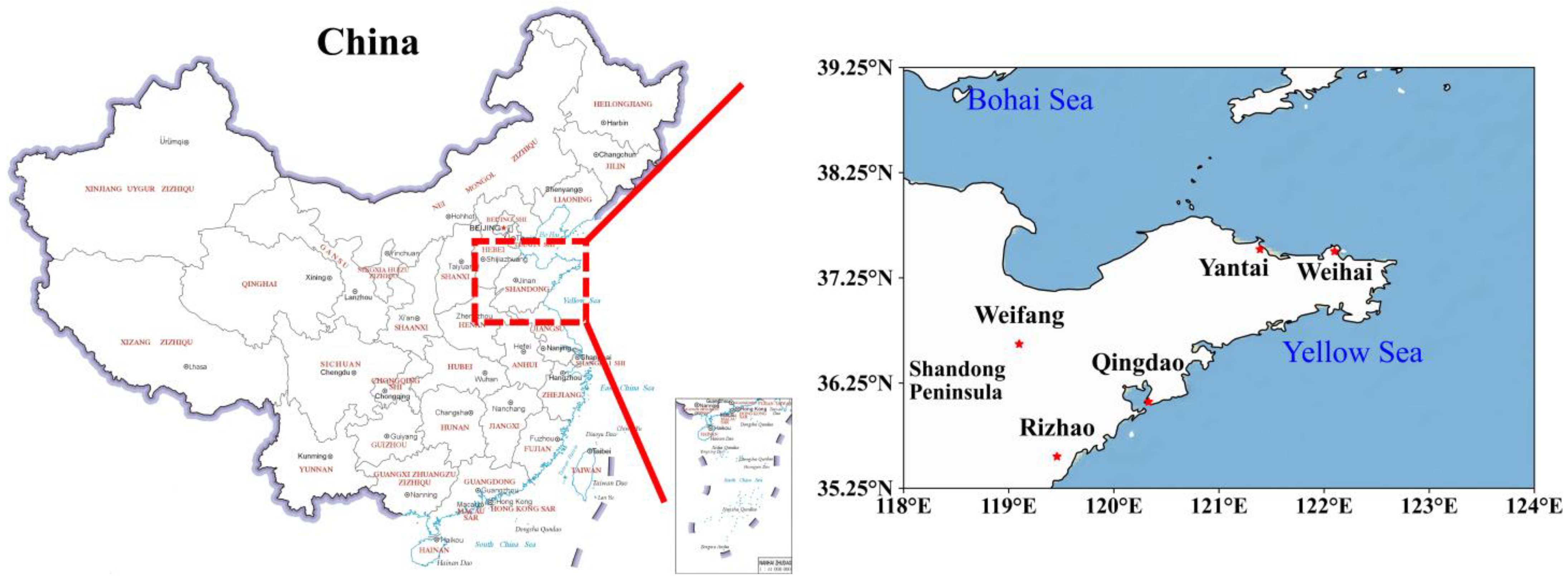
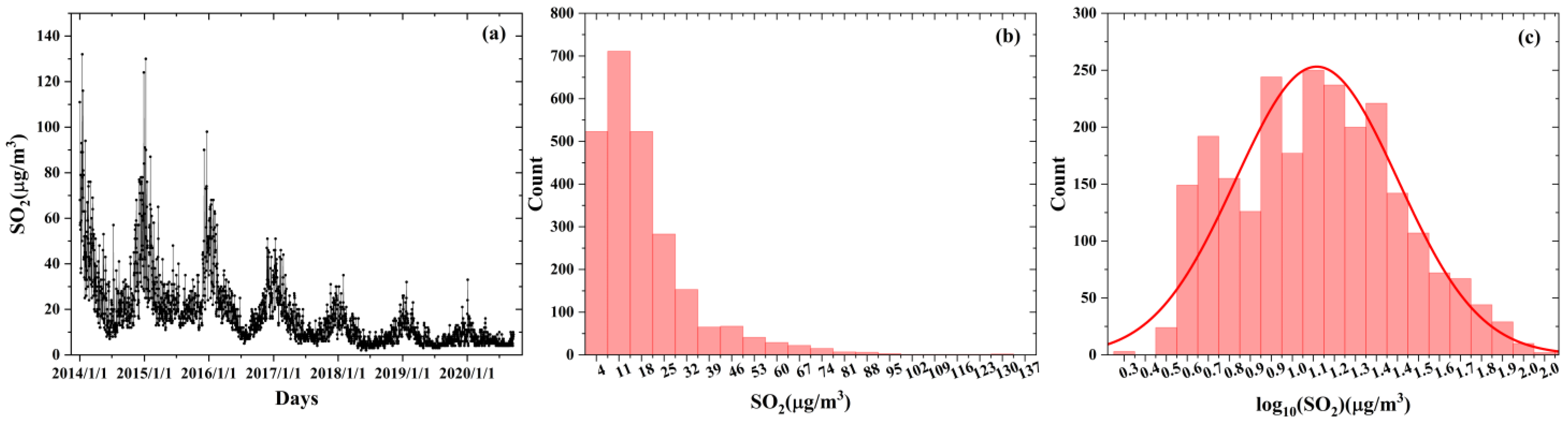
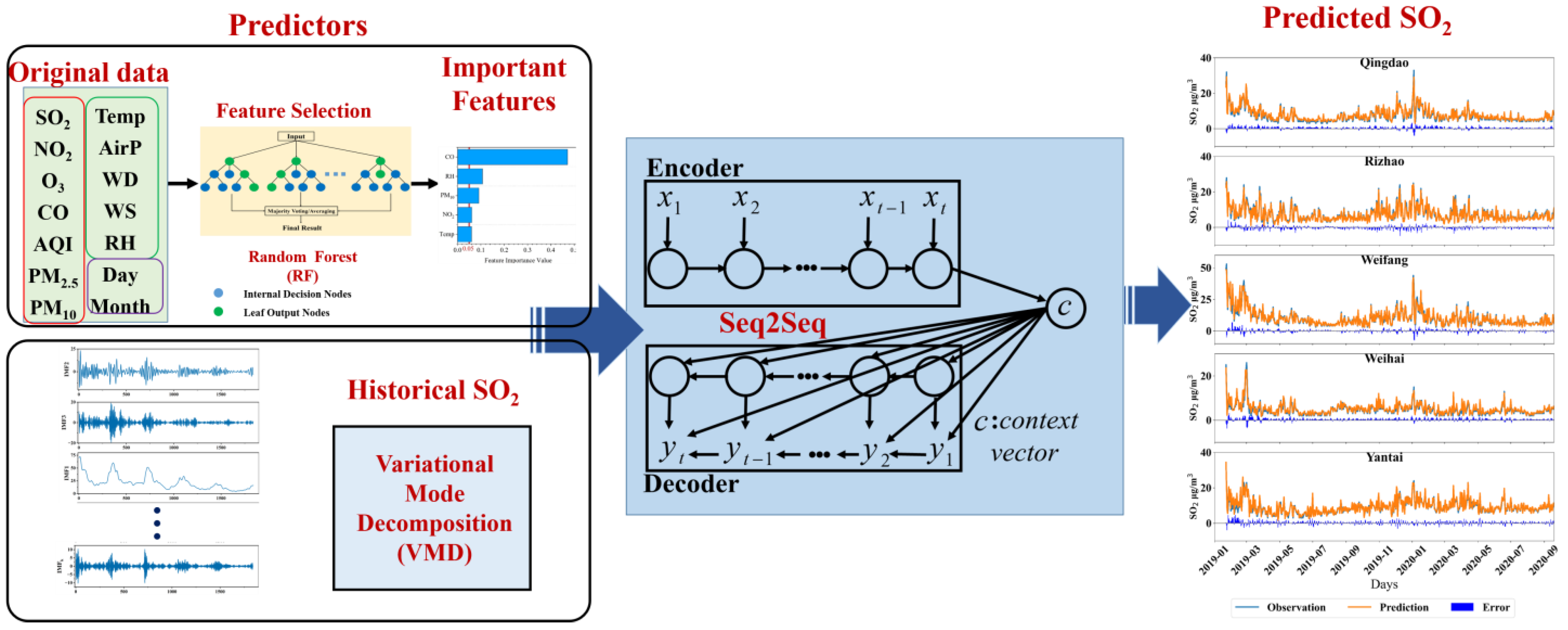
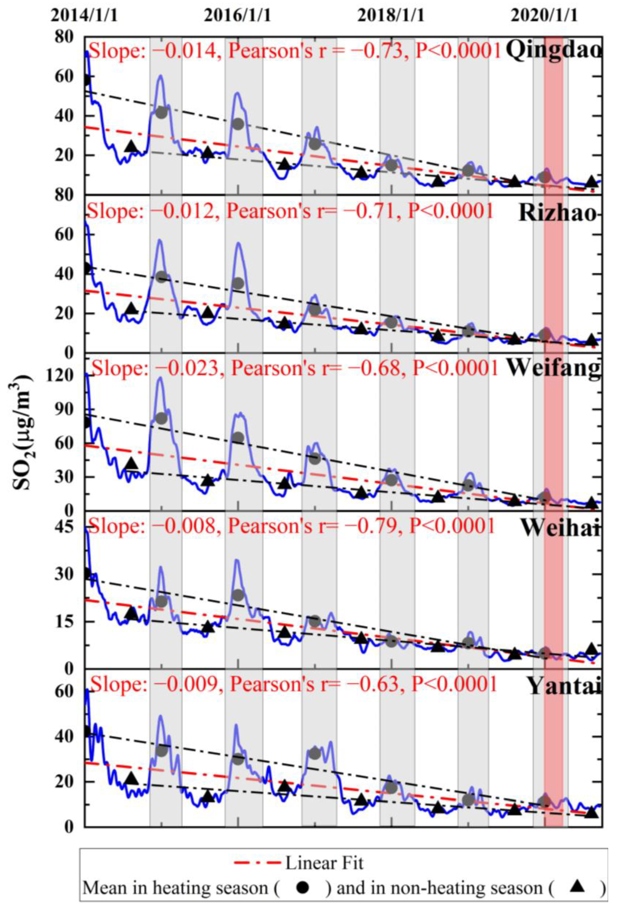
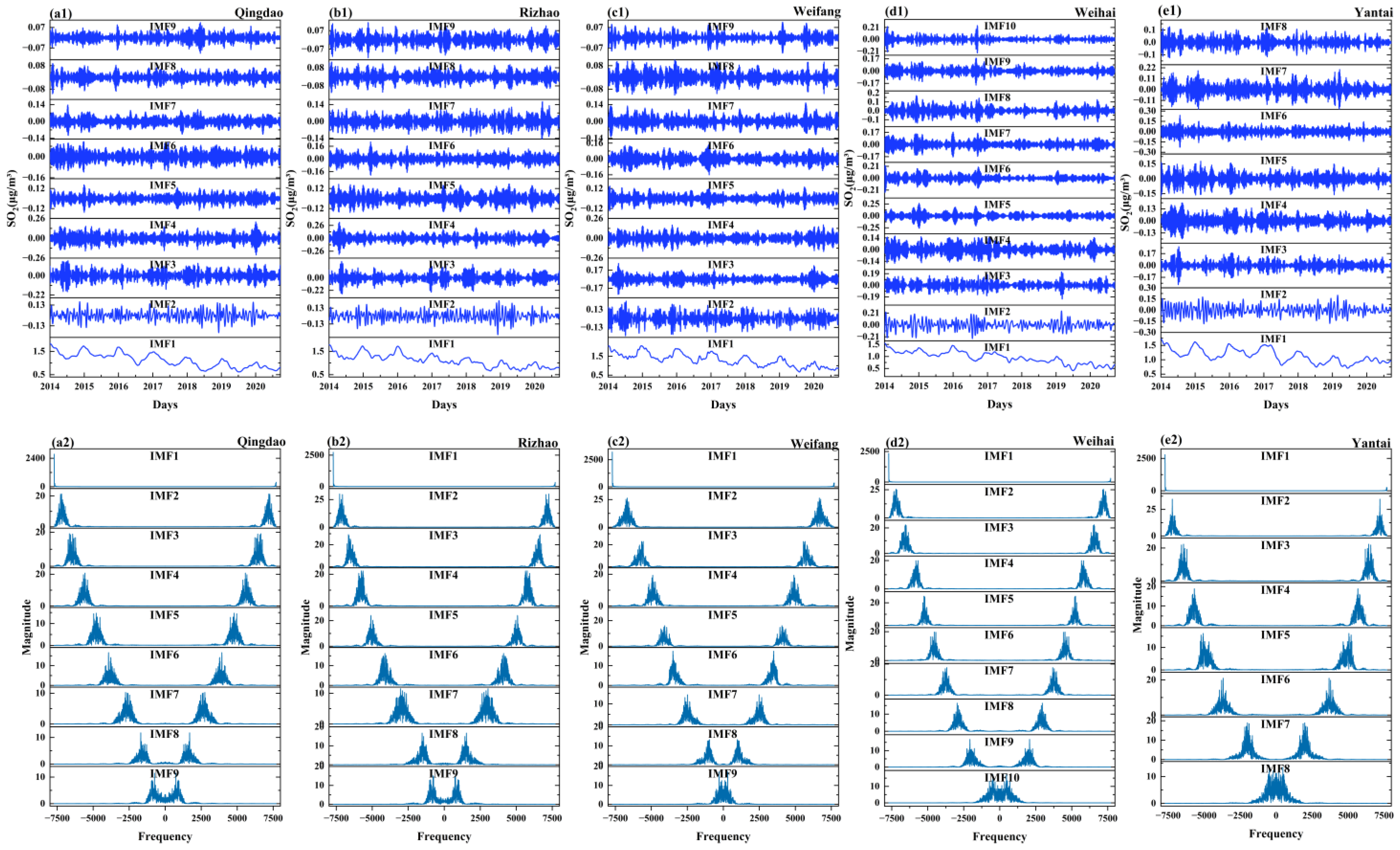
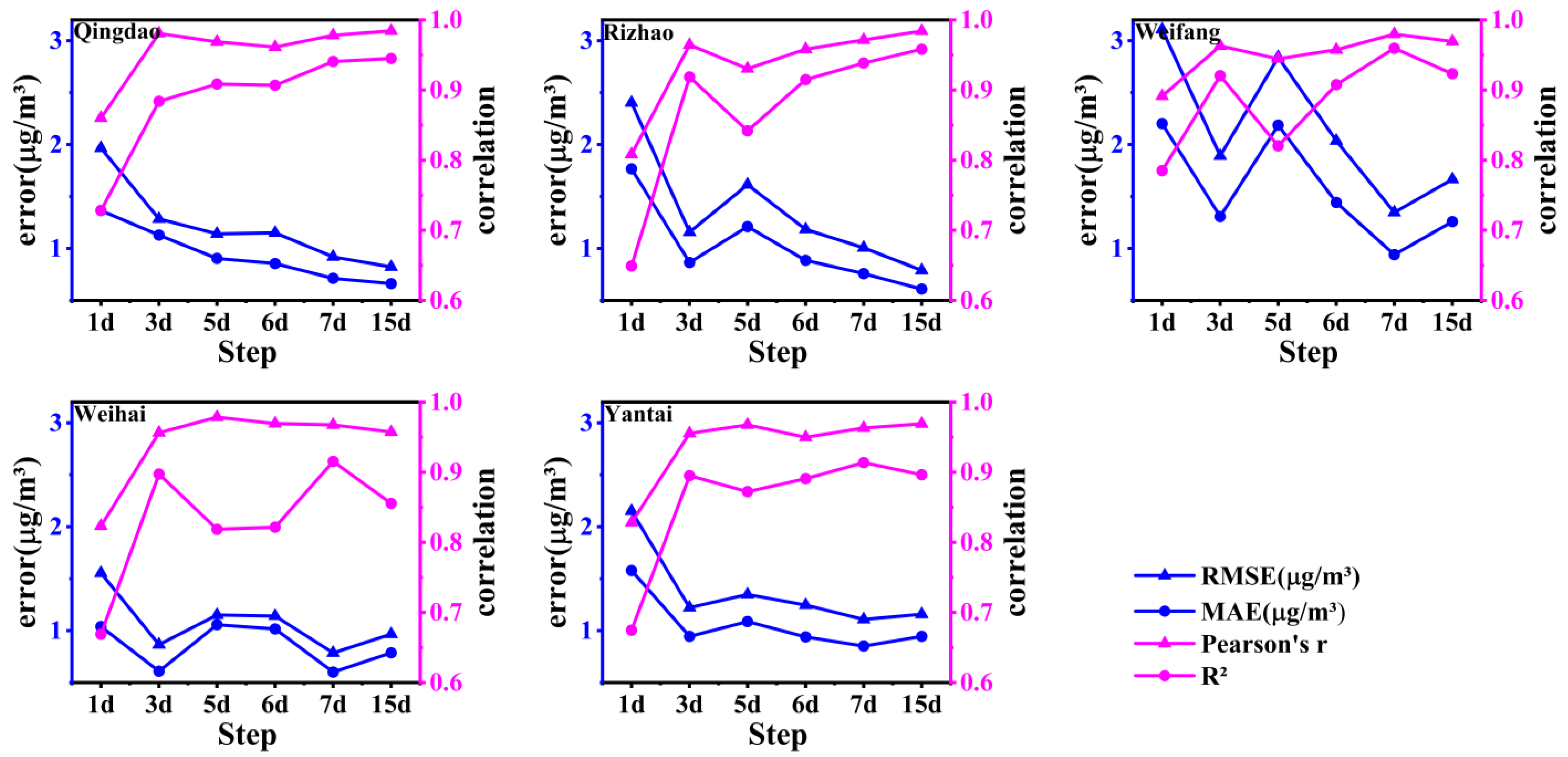
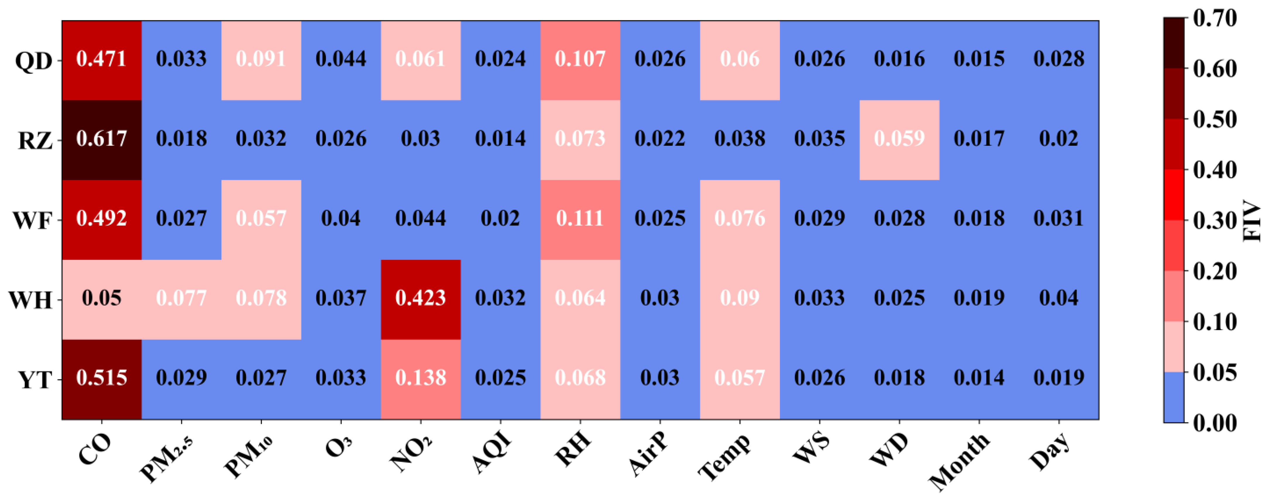
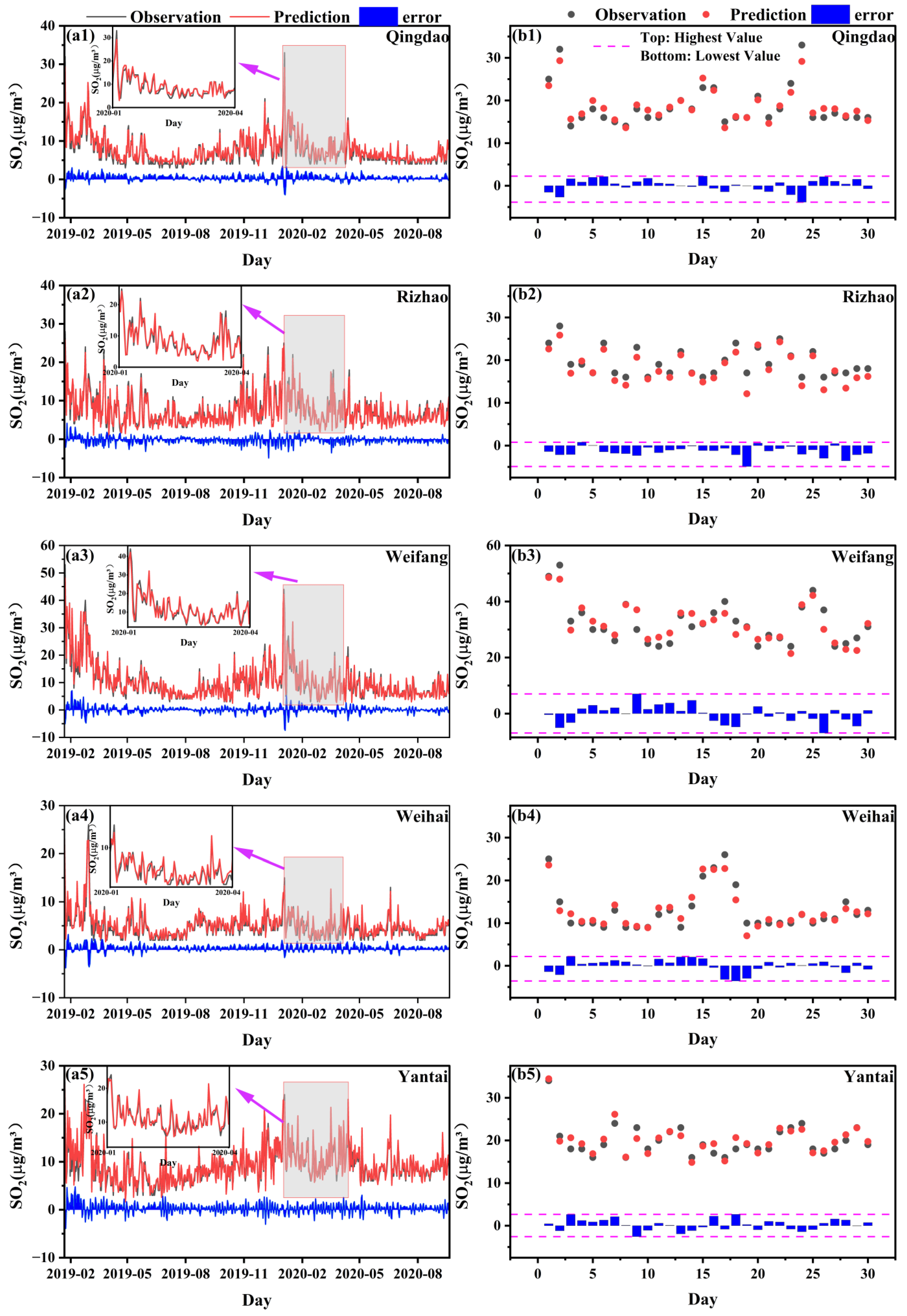
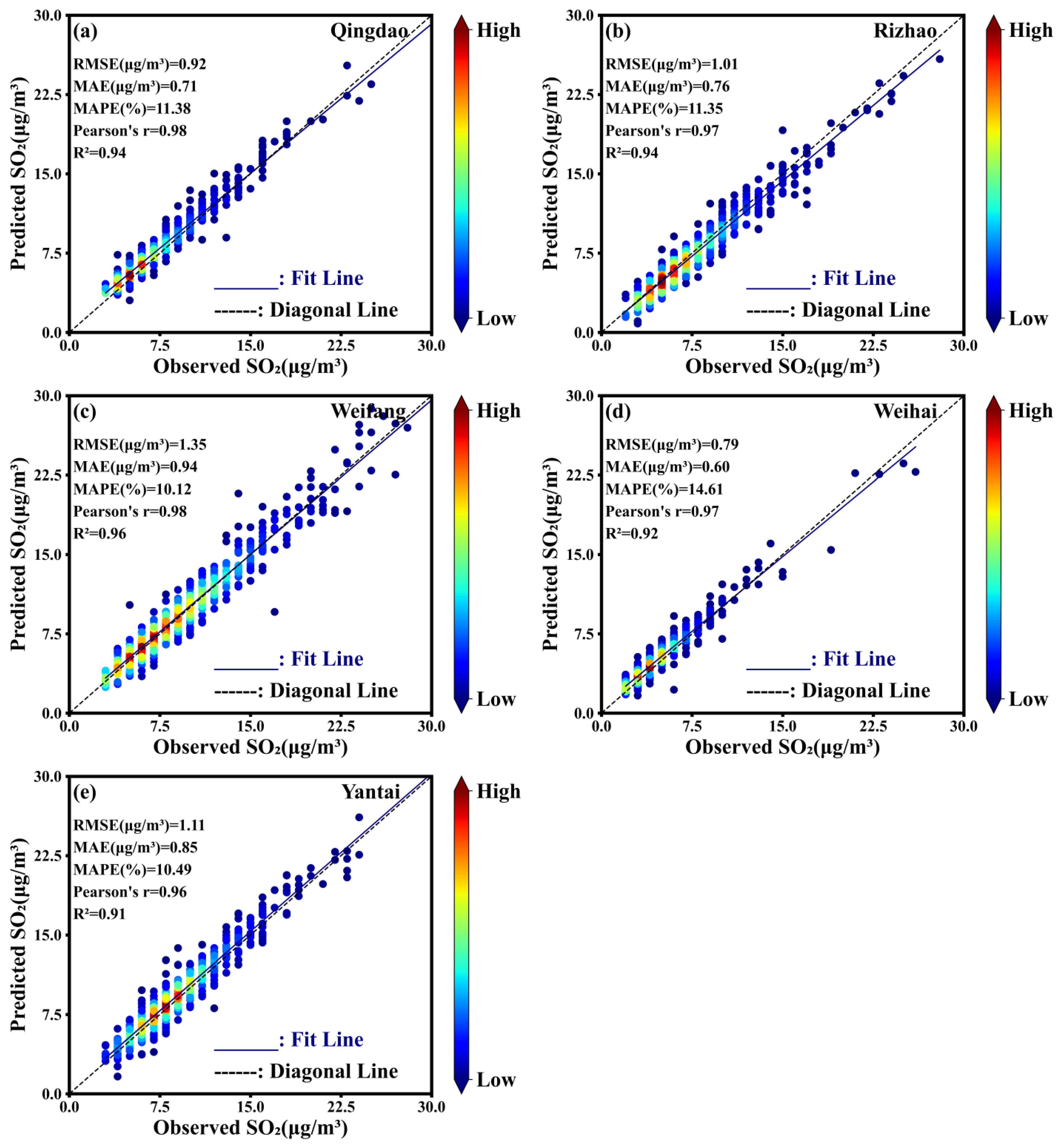
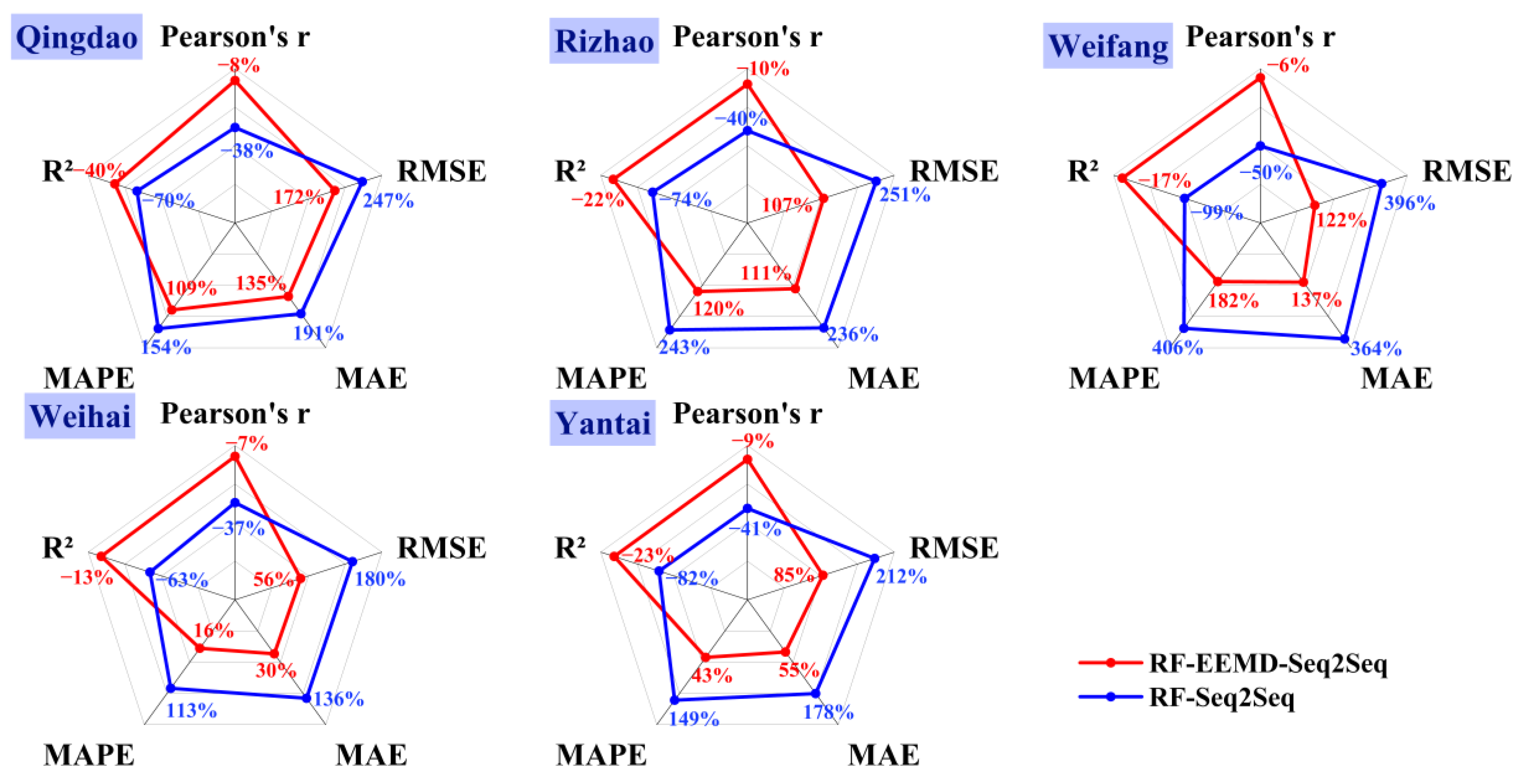
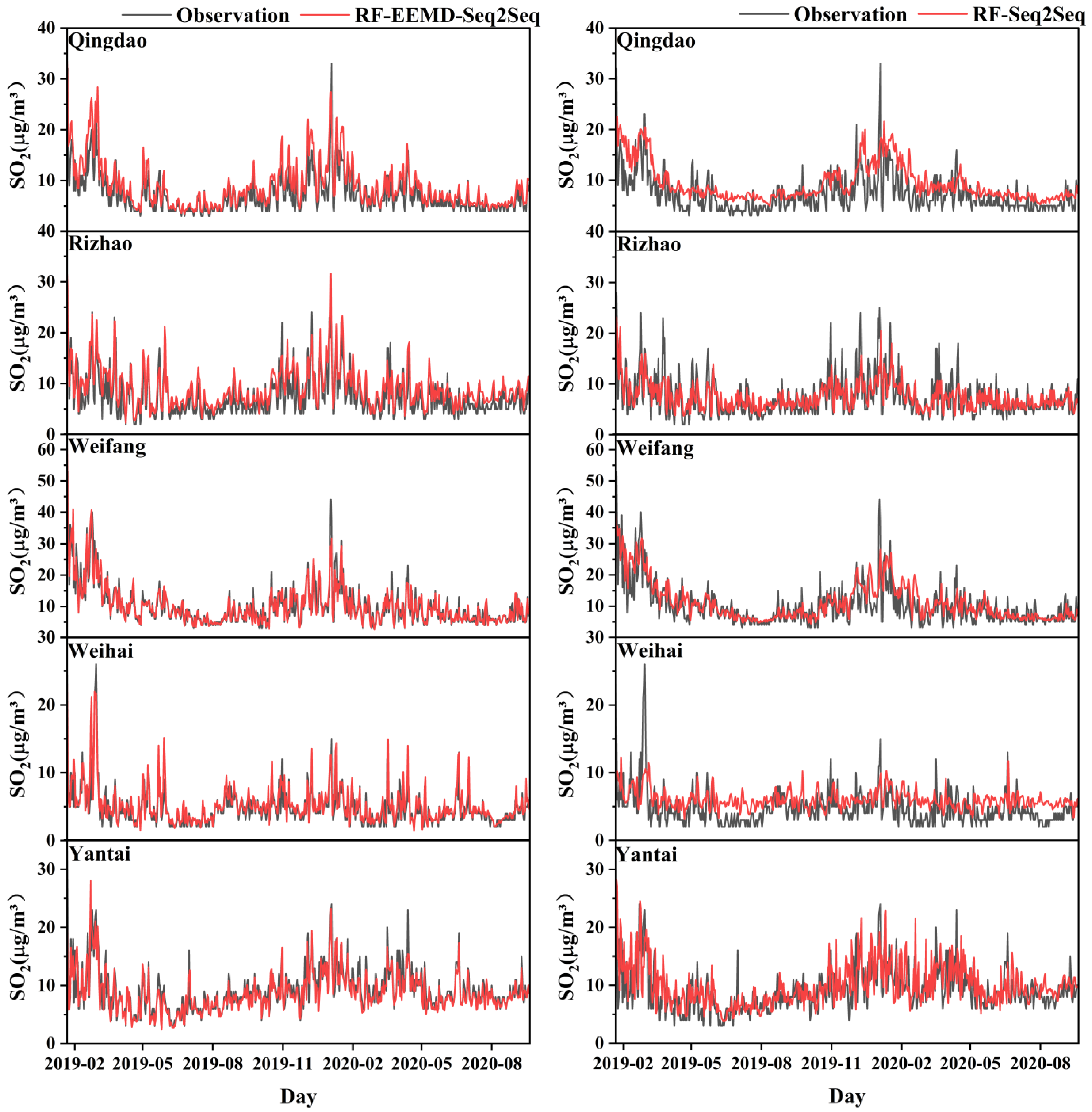
Disclaimer/Publisher’s Note: The statements, opinions and data contained in all publications are solely those of the individual author(s) and contributor(s) and not of MDPI and/or the editor(s). MDPI and/or the editor(s) disclaim responsibility for any injury to people or property resulting from any ideas, methods, instructions or products referred to in the content. |
© 2025 by the authors. Licensee MDPI, Basel, Switzerland. This article is an open access article distributed under the terms and conditions of the Creative Commons Attribution (CC BY) license (https://creativecommons.org/licenses/by/4.0/).