Abstract
This study addresses the procurement problem in mechanical manufacturing enterprises, considering both supply chain disruption risks and carbon emissions. Based on a multi-product, multi-supplier procurement planning optimization problem, a high-dimensional multi-objective optimization model is developed with procurement cost, total loss, number of quality defects, and carbon emissions as objectives. The model is solved using an improved integer-coded NSGA-III algorithm, which includes four mechanisms: heuristic population initialization, infeasible solution optimization and repair, a weight-matrix-based crossover operator, a multi-column exchange mutation operator, and Pareto simulated annealing. Through numerical experiments, the performance of this algorithm is compared with NSGA-III and NSGA-II, demonstrating its superior ability to handle multi-objective, multi-constraint optimization problems. Ablation experiments further validate the effectiveness of the four improved mechanisms. Case study results show that the optimized procurement plan balances economic and environmental benefits while considering supply chain risks.
1. Introduction
With global economic integration, enterprises increasingly rely on external suppliers and cross-border procurement, making global value chains (GVCs) more complex [1,2,3]. The flow of raw materials and intermediate products in global trade exceeds trillions of dollars, with 180 traded products (worth approximately USD 134 billion in 2018) dominated by a single exporting country. While concentrated supply networks reduce management costs, they also increase vulnerability to external shocks. Research shows that supply chain disruptions lasting over a month occur approximately every 3.7 years, with severe cases leading to profit losses equivalent to nearly one year’s earnings [4]. The Russia-Ukraine conflict has further exposed global supply chain fragility, prompting enterprises to reassess supply chain structures and adopt supplier diversification strategies to mitigate risks.
At the same time, carbon reduction policies introduce new complexities to supply chain management. The European Union’s Carbon Border Adjustment Mechanism (CBAM), set to impose carbon tariffs on imports starting in 2026, will increase costs for carbon-intensive industries and may weaken their international competitiveness [5]. Industries such as steel and aluminum, which have high carbon emissions, face rising costs and declining market share. As carbon regulations tighten, enterprises must not only optimize production to reduce their own carbon footprint but also evaluate upstream suppliers’ emissions to ensure environmental compliance.
To mitigate supply chain disruption risks, many enterprises adopt multi-sourcing strategies to reduce dependence on a limited number of suppliers. Research shows that a decade of supply chain disruptions can result in financial losses of up to 42% of annual profits, while multi-sourcing lowers disruption risks [4]. However, this approach also presents challenges. Supply chains account for 80% of total greenhouse gas emissions in consumer goods companies. While supplier diversification reduces supply risks, it may increase carbon emissions from transportation and complicate carbon management. The supply of “green” materials, such as low-carbon steel, remains limited, making it difficult to meet short-term demand in the automotive and manufacturing industries [5]. Conversely, strict carbon compliance may lead to over-reliance on a small number of low-carbon-certified suppliers, heightening concentration risks and weakening supply chain resilience. Balancing environmental benefits and supply chain stability has become a critical challenge in green supply chain management. Addressing this issue requires comprehensive optimization models that integrate economic efficiency, supply chain resilience, and sustainability, enabling coordinated supply chain development.
Existing research on supply chain procurement optimization can be categorized into two main areas. The first focuses on order allocation and procurement strategy optimization. Li et al. [6] proposed a strategy integrating flexible ordering cycles and centralized procurement to reduce costs, while Wu et al. [7] optimized order allocation and financing strategies within a multi-supplier purchase order financing (POF) framework to enhance capital utilization efficiency. Nguyen et al. [8] developed a hierarchical heuristic algorithm to optimize order allocation and batch decision-making by compensating for quality loss and delayed deliveries. The second category addresses integrated supplier selection and order allocation optimization. Ali and Zhang [9] incorporated economic, environmental, and transportation risk factors into a supplier selection model, emphasizing sustainable procurement. Yaghin and Darvishi [10] examined multi-source, multi-product, and multi-transportation-mode order allocation to enhance supply chain resilience. Kuan-Yu et al. [11] developed an integrated evaluation framework combining Z-numbers, game theory, and the ITARA-CoCoSo method to optimize supplier sustainability and order allocation. Bai et al. [12] introduced a multi-objective mathematical optimization model (MOMM) to balance procurement costs, supplier performance, and carbon emission control under carbon neutrality targets. While these studies have yielded valuable insights, they lack a holistic approach that integrates supply chain disruption risks and environmental sustainability into an optimized decision-making framework.
Research on low-carbon policies and environmental sustainability has explored various optimization approaches. Homayouni et al. [13] proposed a robust-heuristic optimization method to simultaneously reduce carbon emissions and supply chain costs. Wang et al. [14] introduced a supplier emission reduction investment strategy and a multi-level backup mechanism under hybrid uncertainty conditions to mitigate carbon emissions and supply risks. Sriklab et al. [15] developed a linear programming model based on evaluation scores to integrate economic, social, environmental, and disruption risk factors in supply chain decision-making. While these studies contribute to sustainable supply chain management, they primarily focus on theoretical model development and lack a comprehensive approach to integrating multi-objective trade-offs with practical applications.
Additionally, research on multi-objective optimization methods has frequently incorporated heuristic and metaheuristic-based approaches. Jadidi et al. [16] developed a mixed-integer nonlinear programming (MINLP) model, integrating supplier selection, quantity discounts, and supply capacity, using a heuristic algorithm for multi-period dynamic pricing and lot-sizing optimization. Yousefi et al. [17] combined data envelopment analysis (DEA) and a Nash bargaining model to optimize supplier selection and order allocation, emphasizing cost-effectiveness trade-offs. Di Pasquale et al. [18] introduced a collaborative allocation curve-sharing mechanism to optimize order allocation under demand uncertainty, incorporating triple-bottom-line criteria. Mangla et al. [19] proposed an emergency order allocation strategy for e-health homecare products during the pandemic. Zhang et al. [20] applied an adaptive large neighborhood search (ALNS) algorithm, a metaheuristic approach, to manage uncertainty in customer order arrivals. Despite these methodological advancements, most studies prioritize algorithmic improvements over practical applicability. They lack empirical validation in supply chain environments and fail to fully address multi-objective coordination under complex constraints.
In recent years, the NSGA family of algorithms has been widely applied to multi-objective optimization in supply chain research due to its strong performance. Ruiz-Vélez et al. [21] conducted a comparative study of NSGA-II, NSGA-III, and RVEA, finding that NSGA-III excels in high-dimensional objective optimization, particularly in maintaining solution diversity and uniformity. Bharadwaj et al. [22] optimized economic costs and social responsibility in the construction supply chain using NSGA-III. Ma et al. [23] improved NSGA-III for ship weather routing problems, enhancing algorithm performance. Cui et al. [24] modified NSGA-II to address load balancing in graph partitioning problems.
Yang et al. [25] integrated market bidding strategies into NSGA-III, proposing adaptive population initialization, optimized reference point association, and dynamic elite selection, which effectively enhanced solution quality and diversity while reducing computational costs. Additionally, Li et al. [26] incorporated tabu search to prevent genetic algorithms from stagnating, while Tang et al. [27] improved genetic algorithm performance through three-layer encoding and heuristic population initialization. Although these studies demonstrate the broad applicability of the NSGA family of algorithms, challenges remain in initial population construction, infeasible solution repair, and real-world validation.
In summary, while existing research has advanced cost control, environmental sustainability, and supply chain risk management, limitations persist in multi-objective optimization for complex supply chains. Most studies focus on individual optimization factors rather than integrating supply disruption risks, quality defects, supplier capacity constraints, and carbon emissions into a coordinated optimization framework, requiring further research. Optimization algorithms require improvements in population initialization, infeasible solution repair, and solution quality under complex constraints. Many studies rely on theoretical models without empirical validation in manufacturing, limiting their practical applicability. To address these research gaps, this study makes the following key contributions:
- Develops a multi-objective optimization model that integrates procurement cost, total loss, defect count, and carbon emissions, incorporating a delayed delivery discount mechanism and a quantitative carbon emission assessment for coordinated optimization.
- Proposes an improved integer-coded NSGA-III(IICNSGA-III)algorithm with enhanced population initialization, infeasible solution repair, weight-matrix-based crossover, multi-column swap mutation, and local convergence control, improving solution efficiency and quality.
- Evaluates the proposed optimization mechanisms through numerical experiments, with a manufacturing case study validating its applicability and advantages in real-world supply chains, supporting both theoretical research and practical applications.
The rest of the paper is structured as follows: Section 2 defines the problem and formulates the mathematical model. Section 3 details the proposed algorithm and its key enhancements. Section 4 presents numerical experiments and performance evaluations, followed by a case study in Section 5 to validate the practical applicability of the approach. Finally, Section 6 concludes the paper and discusses potential directions for future research.
2. Model Construction
2.1. Problem Description
In the procurement process, manufacturing enterprises typically source various types of products from multiple suppliers to meet production demands. However, supplier delivery capacity, product quality, and carbon emissions not only affect procurement costs but also pose potential supply chain disruption risks.
Some suppliers offer price discounts in exchange for longer delivery lead times, but delayed deliveries may disrupt production schedules and result in additional losses. Moreover, supplier quality levels directly impact product defect rates—while lower procurement costs may seem advantageous, purchasing from suppliers with unstable quality can lead to rework, scrap, and increased hidden costs.
With the growing emphasis on green supply chain management, enterprises must also consider supplier carbon emissions in procurement decisions to mitigate the environmental impact of supply chains. Thus, balancing cost reduction, supply risk control, quality stability, and carbon footprint minimization has become a critical challenge in procurement management for manufacturing enterprises.
Against this backdrop, this study develops a multi-objective optimization model for supplier selection and order allocation, considering product demand, supplier capacity, and minimum order quantity constraints. The objectives are the following:
- Minimize procurement costs by incorporating supplier quotations and delayed delivery discounts for a more accurate cost assessment.
- Minimizing supply delay losses by evaluating supplier delivery reliability to mitigate production risks from late deliveries.
- Minimize quality defects by considering supplier defect rates and reducing the impact of quality issues on production.
- Minimize carbon emissions by optimizing procurement based on supplier-specific carbon emission factors, reducing the supply chain’s environmental impact.
This study does not incorporate transportation costs, inventory costs, or supplier reputation, based on the following considerations: transportation costs are typically included in supplier quotations, and optimizing them separately may distort the procurement strategy; inventory costs primarily relate to internal management, which is beyond the core focus of procurement decisions; supplier reputation can be indirectly measured through defect rates and delivery reliability, eliminating the need for additional modeling. By optimizing procurement costs, supply chain risks, quality management, and environmental impact, this study provides a scientifically grounded supplier selection and order allocation strategy for manufacturing enterprises, enhancing supply chain stability and sustainability.
2.2. Model Assumptions
- (1)
- Enterprises incur penalty costs for late deliveries if production delays prevent orders from being completed on time;
- (2)
- The model optimizes order allocation within a single order cycle, where procurement is conducted within a fixed period (e.g., monthly or quarterly);
- (3)
- The same product, when supplied by different suppliers, is assumed to have no significant quality differences;
- (4)
- Each supplier has a limited supply capacity and cannot exceed its maximum delivery volume;
- (5)
- Procurement from suppliers must comply with their minimum order quantity (MOQ) requirements;
- (6)
- Orders can only be allocated to selected suppliers; those not chosen will not receive procurement requests;
- (7)
- Suppliers offer price discounts on parts delivered beyond the agreed delivery period;
- (8)
- A single supplier can provide multiple product types, and the same product within an order may be procured from different suppliers;
- (9)
- Order demand quantities are known and fixed, unaffected by market fluctuations;
- (10)
- The carbon emissions per unit of product are considered constant throughout the procurement process.
In practical procurement management, manufacturing enterprises typically adopt a short-cycle procurement strategy, where purchases are made in phases according to production plans, and decisions for each cycle remain relatively independent. This study assumes a fixed procurement cycle (e.g., monthly or quarterly) based on the following considerations:
- In the short term, supplier prices, delivery capacity, and quality levels remain stable, making single-cycle optimization a more accurate reflection of real-world conditions.
- Procurement discounts, supply contracts, and delivery policies are typically structured on a cycle-by-cycle basis, requiring an optimization approach aligned with enterprise procurement practices.
- Many enterprises adopt a rolling procurement plan, optimizing purchases for each cycle rather than making one-time, long-term procurement decisions.
- Multi-cycle optimization would necessitate additional considerations, including inventory management, market demand fluctuations, and long-term supplier collaboration strategies, significantly increasing model complexity.
Therefore, this study focuses on single-cycle optimization to provide clearer and more direct decision support.
2.3. Objectives
An integer programming model is developed to minimize the manufacturer’s total procurement cost, total supply loss, total defect count, and total carbon emissions during the procurement process.
- Objective Functions
(1) Total Procurement Cost
The objective is to minimize the manufacturer’s total procurement cost, which comprises the cost of on-time deliveries at the original price and the cost of late deliveries at a discounted price.
where i represents the product type, j represents the supplier. Xij is the quantity of product i procured from supplier j, vj is the price discount for late delivered products from supplier j, pij is the unit price of product i offered by supplier j, and lij is the late delivery rate of product i from supplier j.
(2) Total Loss
The objective is to minimize the loss caused by delayed deliveries. Total loss refers to the cost incurred due to supplier delays.
where kij is the unit loss cost per unit time due to delayed delivery, qi is the specified delivery time for product i, and ti is the latest delivery time for product i.
(3) Total Number of Defects
The objective is to minimize the total number of defective products, which is calculated by multiplying the defect rate by the quantity of products procured from the supplier.
where dij represents the defect rate of product i from supplier j.
(4) Total Carbon Emissions
The objective is to minimize the total carbon emissions associated with the transportation process of selected suppliers. It is calculated by multiplying the unit carbon emissions by the quantity of products procured from the supplier.
where gij represents the unit carbon emissions of product i supplied by supplier j.
- 2.
- Model Constraints
(1) The quantity of product i procured from supplier j by the manufacturer must equal its total demand.
where Qi represents the total demand for product i by the company.
(2) Due to the minimum order quantity (MOQ) requirement imposed by supplier j, the quantity of product i procured from supplier j must be greater than or equal to the minimum order quantity.
where mij represents the minimum order quantity of product i at supplier j. zij is a binary variable, indicating whether the product is procured from supplier j.
(3) Due to the supplier’s limited capacity, the total quantity of product i procured from supplier j cannot exceed its maximum supply capacity.
where Cij represents the maximum supply capacity of product i at supplier j.
(4) The quantity of product i procured from supplier j by the manufacturer must be a non-negative integer.
3. Algorithm Design
The order allocation problem is a typical multi-objective optimization problem, where multiple objective functions may conflict with each other. Traditional single-objective genetic algorithms are ineffective in addressing such problems, necessitating the adoption of an appropriate multi-objective optimization algorithm. The NSGA-III algorithm [28] is a widely used heuristic approach for multi-objective optimization, specifically designed for high-dimensional problems. However, NSGA-III primarily relies on floating-point encoding, making it less suitable for integer optimization problems. To enforce integer constraints, additional truncation or rounding operations are often required, which may compromise solution feasibility and affect computational efficiency. Existing studies [29] have acknowledged this limitation and introduced opposition-based learning (OBL) and opposition-based mutation strategies to enhance integer handling in discrete-time-cost-resource tradeoff (DTCRT) problems in construction projects. However, OBL is primarily suited for specific discrete optimization problems and is not directly applicable to the integer-constrained characteristics of the order allocation problem.
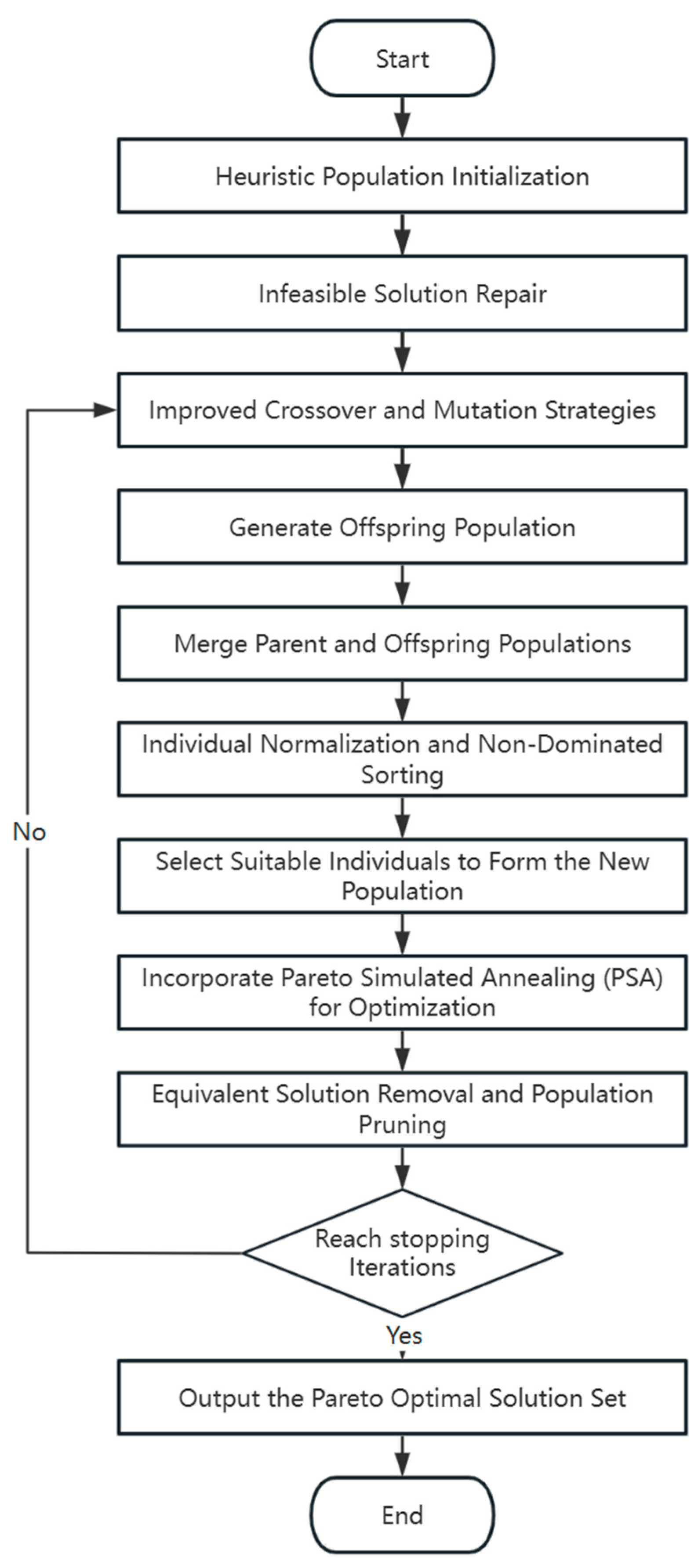
To address these challenges, this study proposes an Improved Integer-Coding Non-dominated Sorting Genetic Algorithm (IICNSGA-III) within the NSGA-III framework. The overall algorithm flow is illustrated in Figure 1.
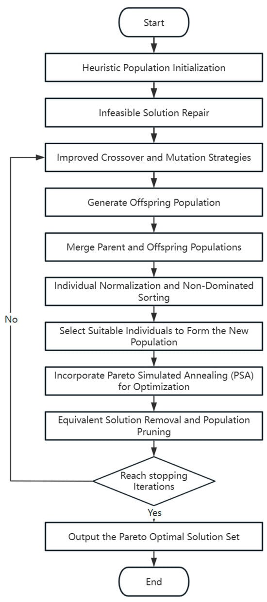
Figure 1.
Flowchart of the IICNSGA-III algorithm.
First, a two-dimensional integer encoding scheme is designed to construct the chromosome structure, where each solution is represented as a two-dimensional matrix, with each element denoting the order quantity allocated between a product and a supplier. During population initialization, a heuristic initialization strategy is implemented, leveraging known supply capacity and minimum order quantity information to construct feasible initial solutions. Additionally, random perturbations are introduced to enhance population diversity and improve the global search capability of the algorithm. Subsequently, infeasible solutions are identified and repaired before proceeding to the evolutionary phase.
During the evolutionary process, traditional crossover and mutation strategies in genetic algorithms often fail to effectively handle integer constraints. To overcome this, this study introduces a weight-matrix-based crossover operator and a multi-column swap mutation operator, ensuring integer feasibility while maintaining solution diversity. Additionally, Pareto Simulated Annealing (PSA) is integrated into the framework to perform local optimization on the current Pareto solution set in each generation. The Metropolis criterion is employed to determine whether to accept a new solution, allowing for the acceptance of inferior solutions in the early search stages to escape local optima, while gradually refining the solution as the temperature decreases, ultimately converging toward the global optimal solution. The final output is the optimal order allocation scheme that satisfies all constraints.
In summary, the proposed IICNSGA-III algorithm integrates Heuristic Population Initialization, Infeasible Solution Repair, Weight-Matrix Based Crossover, Multi-Column Swap Mutation, and Pareto Simulated Annealing. This approach aims to improve solution quality, enhance solution diversity, and ensure compliance with complex supply chain constraints.
3.1. Heuristic Population Initialization
In this study, an integer encoding method is used to construct the chromosome structure, where each chromosome is a one-dimensional integer vector. The chromosome’s fitness value corresponds to the objective function value of the model. The vector is reshaped into an I × J matrix, where I represents product types, J represents suppliers, and each element xij represents the quantity of product i allocated to supplier j.
To enhance population diversity and mitigate premature convergence, we incorporate random perturbations during initialization. This approach is inspired by the Random Strategy (RS) in dynamic multi-objective optimization [30], where controlled variations around centroids help maintain diversity. Unlike RS, which perturbs a single centroid, our method introduces independent perturbations to each individual within [−50, 50], ensuring broader exploration of the solution space.
The initial population is generated through a structured heuristic approach that ensures feasibility while maintaining diversity. First, the total demand for each product is computed and evenly distributed among suppliers. To introduce randomness, the supplier order is shuffled. Next, minimum order constraints are enforced by setting order quantities below the threshold to zero, and a supplier selection matrix is generated.
To account for capacity constraints, order allocations are adjusted to ensure that all values remain within supplier capacity limits. A random matrix U ∈ [0, 1] is then generated, and for elements where U ≤ 0.6, perturbations in the range [−50, 50] are applied, introducing controlled variability while preserving feasibility. Finally, a repair mechanism ensures that all order quantities are non-negative integers and within supplier capacity constraints. The process continues iteratively until population initialization is complete.
The detailed procedure is described in Algorithm 1.
| Algorithm 1: Heuristic Population Initialization |
| Input: Orders, suppliers, demands, capacities, population size N |
| Output: Initial population P |
| 1: P ← [] |
| 2: for i = 1 to N do |
| 3: A ← initialize_allocation(demands, suppliers) |
| 4: shuffle_suppliers(A) |
| 5: enforce_min_order(A) |
| 6: enforce_capacity(A) |
| 7: U ← random_matrix(0,1) |
| 8: A[U ≤ 0.6] += random(−50,50) |
| 9: repair(A) |
| 10: P.append(A) |
| 11: end for |
| 12: return P |
3.2. Infeasible Solution Repair
To ensure feasibility and compliance with production constraints, the procurement plan undergoes constraint-based optimization and repair, adhering to Equations (5)–(8). The repair mechanism is designed to eliminate infeasible solutions while maintaining solution diversity and stability throughout the optimization process.
This approach is inspired by the Dynamic Constraint Relaxation Mechanism (DCRM) [31]. However, unlike DCRM, which gradually relaxes constraint thresholds and allows mildly infeasible solutions to evolve, the proposed method strictly enforces feasibility at all stages. Rather than tolerating constraint violations, infeasible solutions are dynamically adjusted during optimization to enhance search efficiency and improve solution stability. By prioritizing feasibility early in the process, the algorithm prevents convergence to infeasible regions while preserving exploration capability.
The repair procedure begins by computing the total allocated demand for each product. Order quantities that fall below the minimum order threshold, mij are set to zero, and allocation is prioritized for suppliers with the highest remaining capacity. If unmet demand exists, it is reassigned to suppliers in descending order of available capacity, with an element of randomized allocation to enhance solution diversity.
To maintain capacity feasibility, order quantities are adjusted to ensure they remain within supplier limits:
where Lj and Uj denote the lower and upper capacity limits for supplier j, respectively. The repair mechanism further ensures integer feasibility by applying rounding and clipping operations, maintaining valid order quantities while preserving feasibility constraints.
Finally, the supplier selection matrix zij is updated based on the repaired solution. Only suppliers meeting the minimum order requirement are retained, ensuring that the final repaired solution satisfies all constraints.
The detailed procedure is described in Algorithm 2.
| Algorithm 2: Infeasible Solution Repair |
| Input: Infeasible solution x |
| Output: Repaired feasible solution x |
| 1: for each order j do |
| 2: If allocated_vol(j) > demand(j) then reduce allocation |
| 3: If allocated_vol(j) < demand(j) then record shortfall |
| 4: end for |
| 5: for each supplier k do |
| 6: If assigned_vol(k) > capacity(k) then reassign excess |
| 7: end for |
| 8: for each underallocated order j do |
| 9: assign remaining volume to suppliers with spare capacity |
| 10: end for |
| 11: return x |
3.3. Crossover and Mutation Strategy
In evolutionary computation for integer optimization, crossover operators facilitate the effective transmission of genetic information, while mutation operators play a crucial role in maintaining population diversity and preventing premature convergence. However, traditional crossover and mutation strategies face inherent limitations in integer optimization problems. For instance, Simulated Binary Crossover (SBX) may generate non-integer offspring, violating problem constraints, while polynomial mutation struggles to explore integer search spaces effectively [32].
To overcome these challenges, this study employs a weighted gene recombination strategy and a structured gene exchange mechanism, refining crossover and mutation operations to enhance feasibility and search efficiency. By controlling the fusion of integer chromosome variables in crossover and optimizing the mutation process of integer variables, the proposed method improves solution quality while maintaining feasibility.
- (1)
- Weight-Matrix Based Crossover
This crossover operator leverages a weight matrix to generate offspring while ensuring integer feasibility. Two individuals are selected as parents, and if there are insufficient parents, the current individual is retained for the next generation. A random number is drawn from [0, 1] to determine whether crossover should occur, based on a predefined probability Pc. If crossover is performed, a weight matrix W is constructed with dimensions matching the chromosome structure, where each element is sampled uniformly from [0, 1]. This matrix regulates the contribution of genes from each parent.
Offspring chromosomes are generated as a weighted combination of the parent chromosomes, followed by rounding to the nearest integer to maintain feasibility. Constraints are then enforced to ensure that the offspring remain within the allowable solution space. This process is applied to all selected parent pairs until the entire population undergoes crossover. The detailed procedure is presented in Algorithm 3.
| Algorithm 3: Weight-Matrix Based Crossover |
| Input: Parents P1, P2, crossover probability Pc |
| Output: Offspring O |
| 1: Generate r ∈ [0, 1] |
| 2: if r > Pc then |
| 3: O ← P1 or P2 (no crossover) |
| 4: return O |
| 5: end if |
| 6: W ← random_matrix(0,1) |
| 7: O ← P1 * W + P2 * (1 − W) |
| 8: return O |
- (2)
- Multi-Column Swap Mutation
Following crossover, mutation is introduced to enhance search efficiency while preserving integer feasibility. Unlike polynomial mutation, which perturbs genes without guaranteeing integer constraints, this method swaps genes within the chromosome to maintain feasibility. A random number is drawn from [0, 1] for each individual, determining whether mutation occurs based on the predefined mutation probability Pm.
For individuals undergoing mutation, two positions in the chromosome are randomly selected, and their values are exchanged. This approach diversifies the population while ensuring that the solution remains valid. The mutation process is applied iteratively to all individuals in the population. The detailed procedure is presented in Algorithm 4.
| Algorithm 4: Multi-Column Swap Mutation |
| Input: Solution x, mutation probability Pm |
| Output: Mutated solution x |
| 1: for each individual x in X do |
| 2: Generate r ∈ [0, 1] |
| 3: if r ≤ Pm then |
| 4: Randomly pick u, v from x |
| 5: Swap x[u] and x[v] |
| 6: end if |
| 7: end for |
| 8: return X |
3.4. Pareto Simulated Annealing
Simulated Annealing (SA) is widely used in multi-objective optimization for local search and avoiding local optima. Previous studies [33] have integrated SA with temperature control mechanisms to dynamically adjust the search range while using the Metropolis criterion to enhance search efficiency. This approach has demonstrated a strong global-local search balance in hybrid optimization algorithms such as PSO-DE.
Inspired by this, the proposed Pareto Simulated Annealing (PSA) method introduces a temperature decay coefficient α to gradually reduce perturbation intensity, thereby refining the search space. The Metropolis criterion is employed to determine the acceptance probability of new solutions, ensuring the quality and uniformity of the Pareto front.
The algorithm begins with an initial temperature T0 and iteratively explores the solution space through neighborhood perturbations. Given a current solution x, a new solution x’ is generated by randomly modifying one of its decision variables. The new solution’s objective values are then computed and compared with those of the current solution.
The Metropolis criterion dictates whether x’ replaces x:
where and represent the total objective values of x’ and x, respectively. A random number r is generated from U(0,1). If r < p, the new solution is accepted; otherwise, the current solution is retained.
If x’ is accepted and is non-dominated, it is added to the Pareto solution set. To progressively refine the search space and improve solution stability, the temperature is gradually decreased using the following cooling function:
The process continues until the temperature reaches Tmin or the maximum number of iterations is reached. The final Pareto front is constructed by filtering out dominated solutions. The detailed procedure is presented in Algorithm 5.
| Algorithm 5: Pareto Simulated Annealing |
| Input: Initial solution x, initial temperature T0, minimum temperature Tmin, max iterations tmax, cooling factor α |
| Output: Pareto set P |
| 1: T ← T₀; t ← 0; P ← {x} |
| 2: while T > Tₘᵢₙ and t < tₘₐₓ do |
| 3: x’ ← perturb(x) |
| 4: , ← compute_objective(x’), compute_objective(x) |
| 5: p ← 1 if ≥ else exp(( − )/T) |
| 6: if rand() < p then |
| 7: x ← x’ |
| 8: if x’ is non-dominated then |
| 9: P ← P ∪ {x’} |
| 10: end if |
| 11: T ← α ⋅ T; t ← t + 1 |
| 12: end while |
| 13: return P |
3.5. Complexity Analysis
It can be seen that the main computational cost of IICNSGA-III in each iteration is spent on the non-dominated sorting, variation operations (crossover, mutation, repair), fitness evaluations, and Pareto Simulated Annealing (PSA) for local refinement. The algorithm combines parent and offspring populations of size N and applies fast non-dominated sorting, which typically runs in time, or if M is the number of objectives. Each individual undergoes crossover and mutation, involving D decision variables such as integer-coded genes and capacity constraints. This step takes time. The repair operator, which ensures feasibility, also runs in . The multi-objective fitness evaluation of each individual requires O(T) operations, where T includes both objective function computations and constraint checks. Since there are N individuals per generation, the total cost for this step is . Unlike standard NSGA-III, IICNSGA-III integrates PSA as a key refinement step. Each elite solution undergoes k iterations of local search, leading to an additional cost of per generation, where E is the number of elite solutions.
To sum up, the time complexity of IICNSGA-III iteration is .
4. Numerical Experiments and Analysis
In this section, numerical experiments are conducted to evaluate the overall performance of the proposed IICNSGA-III algorithm. All algorithms are implemented in Python 3.12.1 and executed on a computer with an Intel Core i7-10510U processor (2.30 GHz) (Lenovo, Beijing, China), running Windows 11.
4.1. Experimental Dataset
Since no standard benchmark dataset exists for procurement plan optimization problems, problem instances were constructed based on the problem’s characteristics using different parameter combinations. Each instance is defined by two key parameters: I (number of product types) and J (number of suppliers). To maintain consistency, instances are labeled as “number of product types—number of suppliers”, as shown in Table 1. Given the inherent randomness of heuristic algorithms, experimental results can be sensitive to dataset characteristics, potentially affecting accuracy. To ensure a comprehensive performance evaluation, nine datasets were generated, covering different instance scales. These datasets include supplier counts of 5, 10, and 15, and product counts of 10, 20, and 30.

Table 1.
Description of problem instances.
The distribution and specific values of the parameters used in the problem instances are provided in Table 2. Here, U represents a uniform distribution. For parameters following multiple distributions, such as , the corresponding distribution type is assigned cyclically based on the number of product types. For example, the first product type follows U(20, 40), the second product type follows U(60, 100), and so forth. When the fourth product type is reached, the first distribution type is selected again, and this cycle repeats until all problem parameters for all product types are generated.
Table 2.
Model Parameters and Corresponding Distributions.
4.2. Performance Comparison Experiment
The performance of the proposed IICNSGA-III algorithm is evaluated by comparing it with NSGA-III and NSGA-II algorithms. The algorithm parameters are set as follows: population size = 120, maximum number of iterations = 500, crossover probability = 0.9, and mutation probability = 0.1. To ensure a fair comparison, all three algorithms are tested on nine problem instances, and the objective function values obtained are analyzed. Each algorithm is executed 10 times for each problem instance to mitigate the impact of randomness.
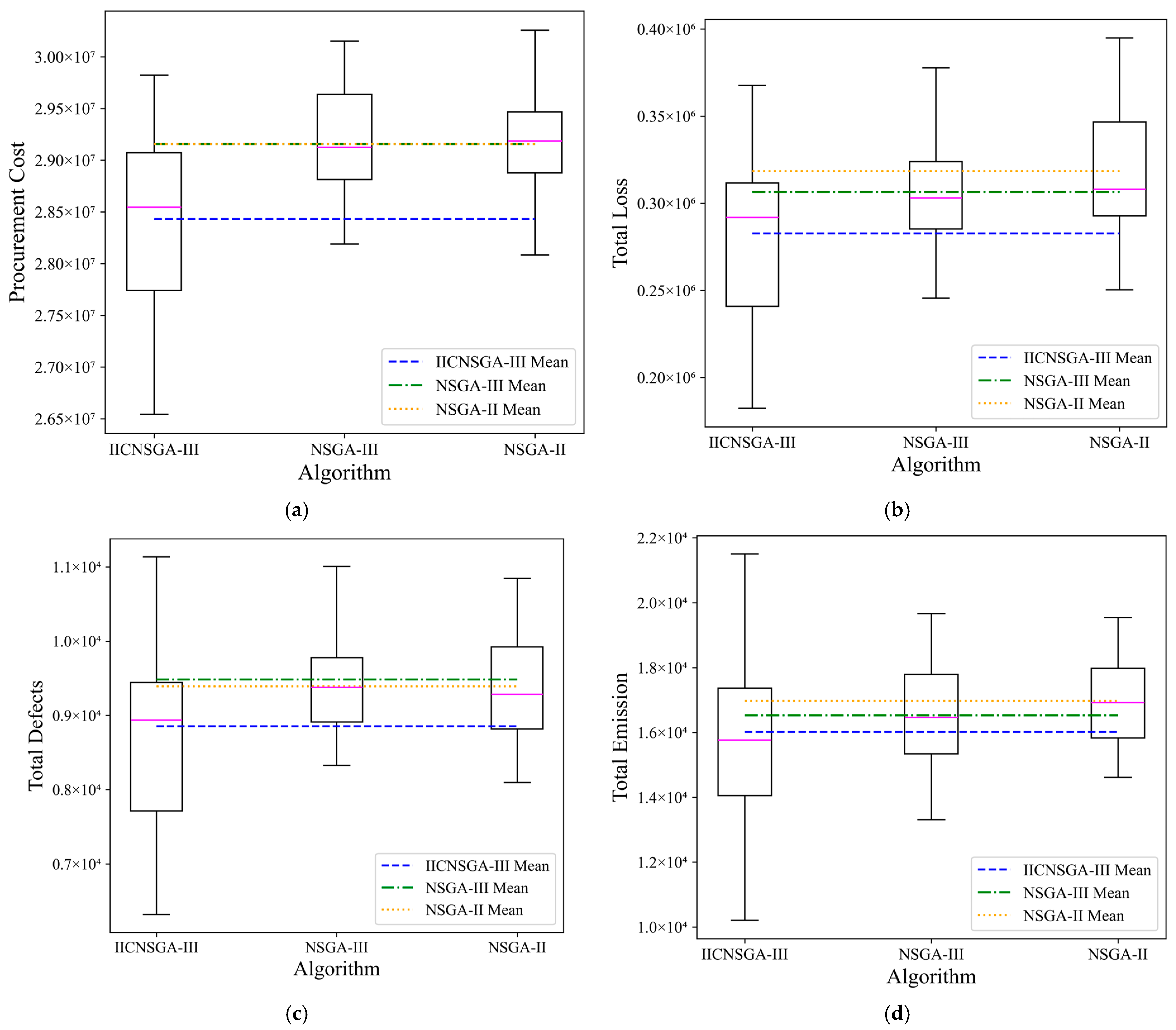
Box plots are used to illustrate the objective function values obtained by IICNSGA-III, NSGA-III, and NSGA-II for both small-scale and large-scale instances, providing a performance evaluation of the IICNSGA-III algorithm. Figure 2 and Figure 3 present the results for instances 10-15 and 30-15, respectively, comparing the performance of the three NSGA algorithms in solving the multi-objective procurement optimization model. Each subplot contains three box plots, representing the performance of the multi-objective procurement optimization model optimized by the three NSGA algorithms. Each box plot includes four black horizontal lines and one pink horizontal line, which indicate the maximum value, upper quartile, lower quartile, minimum value, and median of the solution set, respectively. Additionally, each subplot features three long dashed lines representing the mean values of the solution sets obtained by the three NSGA algorithms.
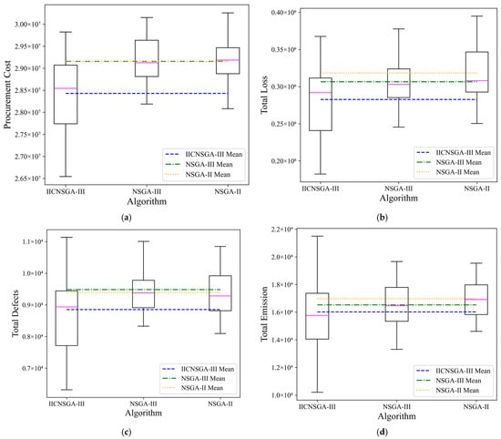
Figure 2.
Performance comparison of three algorithms on four procurement optimization objectives in the 10-15 instances: (a) procurement cost; (b) total loss; (c) total defects; and (d) total emission.
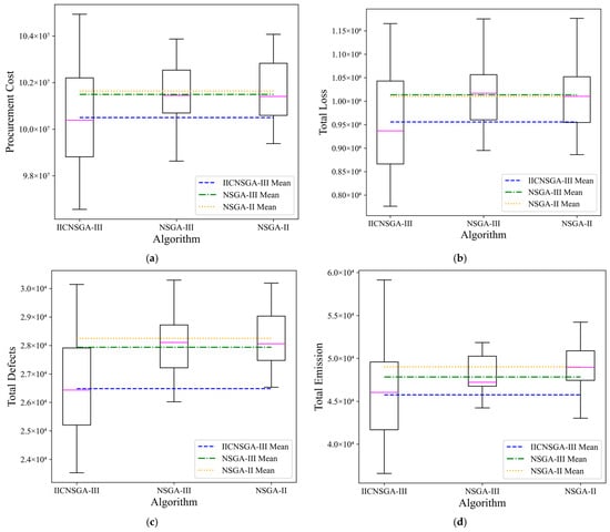
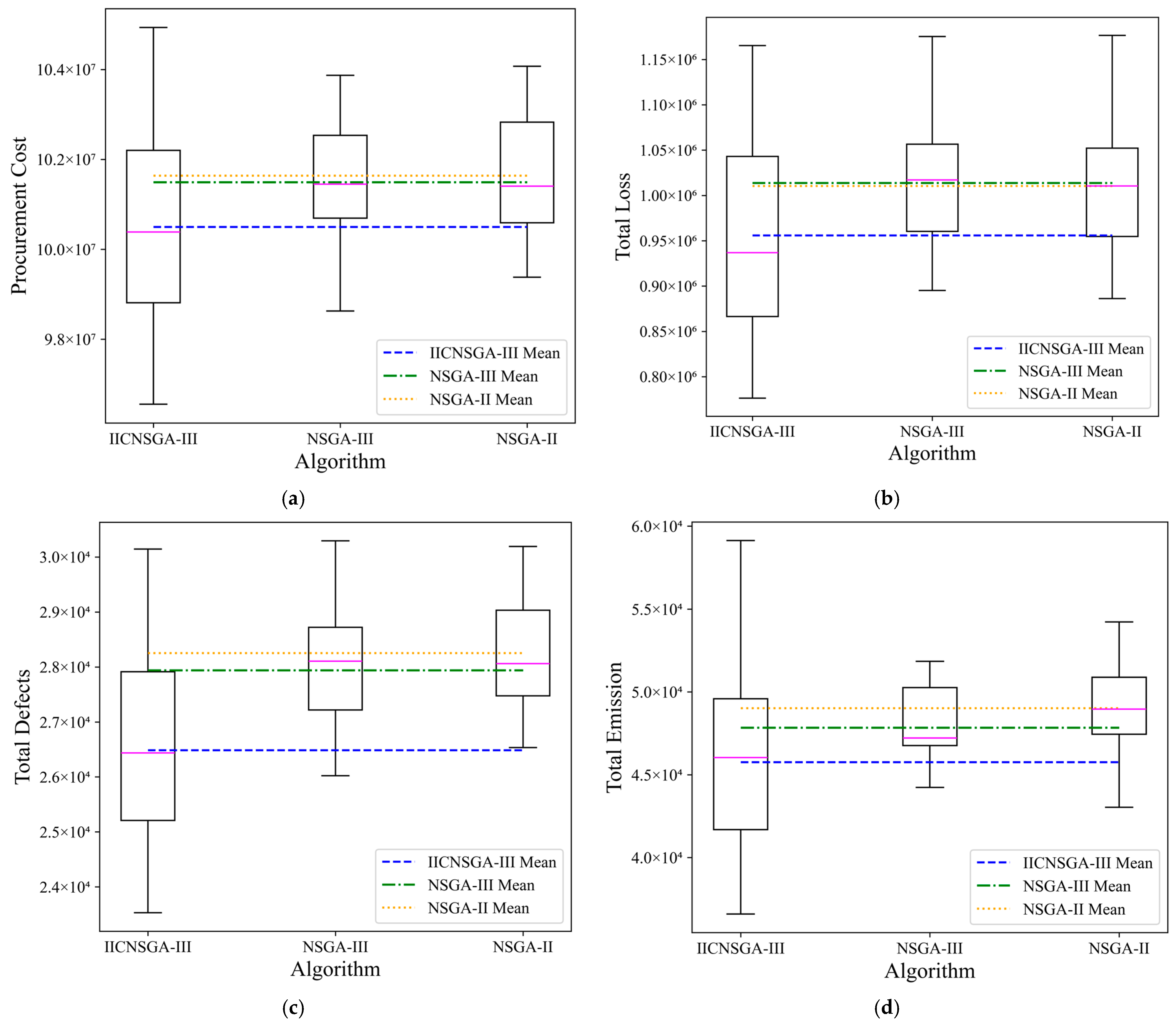
Figure 3.
Performance comparison of three algorithms on four procurement optimization objectives in the 30-15 instance: (a) procurement cost; (b) total loss; (c) total defects; and (d) total emission.
Figure 2 and Figure 3 show that for both small-scale and large-scale instances, IICNSGA-III yields lower mean and minimum values for all four objective functions compared to NSGA-III and NSGA-II. Moreover, as the problem size increases, IICNSGA-III consistently maintains a significant advantage, demonstrating its superior solution quality over NSGA-III and NSGA-II. Specifically, as the number of products and suppliers increases, IICNSGA-III consistently finds lower objective function minima while keeping the upper bound (i.e., maximum value) from increasing significantly. Additionally, the median and mean values of all four objective functions in the solution sets are lower in IICNSGA-III than in NSGA-III and NSGA-II, demonstrating the superior overall performance of the proposed algorithm.
In contrast to the other two algorithms, IICNSGA-III exhibits a slightly more dispersed solution distribution. This is closely linked to the nature of the multi-objective optimization model, which simultaneously considers economic, quality, risk, and environmental objectives. In such cases, the algorithm must navigate trade-offs among competing objectives, where optimizing one may come at the expense of another.
For instance, by minimizing procurement costs, the algorithm may favor lower-cost suppliers, even if they have longer delivery times or lower quality standards. This trade-off can increase total loss and defect rates, reducing robustness in these aspects. Nevertheless, despite these compromises, IICNSGA-III consistently achieves lower mean and minimum values across all objective functions. This demonstrates its ability to effectively balance competing goals, avoiding excessive optimization in a single area while ensuring a well-rounded solution that integrates economic efficiency, quality, risk mitigation, and environmental considerations.
To compare the optimization results of different algorithms, the Relative Percentage Deviation (RPD) is used as a metric to assess solution quality among the three algorithms. The RPD is calculated using the following formula:
where D(A) represents the objective function value obtained by algorithm A for problem instance D, and Dbest denotes the best objective function value among the results obtained by the three algorithms for the same problem instance D. Since a lower objective function value corresponds to a more optimal procurement plan, RPD is always greater than or equal to zero. A smaller RPD indicates that the solution is closer to the optimal result, and RPD = 0 signifies that the solution is the best among all computed results. For the nine problem instances, the proposed algorithm is compared with other algorithms based on the relative percentage deviation of the minimum value (MIN), the maximum value (MAX), and the average of the best values (AVG) obtained from 10 independent runs within five sets of trials for each problem instance. The corresponding results are presented in Table 3.
Table 3.
Relative percentage deviation (RPD) of three algorithms across nine problem instances.
From Table 3, it can be observed that in the vast majority of problem instances, the minimum (optimal) and mean Relative Percentage Deviation (RPD) values obtained by the IICNSGA-III algorithm are zero, indicating that the solution quality of IICNSGA-III is superior to that of NSGA-III and NSGA-II.
Specifically, the RPD values of both the best-found solutions and the mean solutions obtained by IICNSGA-III are significantly lower than those of NSGA-III and NSGA-II across all test cases. This improvement is primarily attributed to structural enhancements in IICNSGA-III, particularly the incorporation of repair mechanisms in population initialization, crossover, and mutation operations. By ensuring that the generated solutions consistently satisfy integer constraints and other problem-specific conditions, IICNSGA-III effectively enhances solution feasibility and robustness. This is particularly crucial for the order allocation problem, which involves a large solution space with multiple constraints.
In addition to structural improvements, IICNSGA-III integrates the NSGA-III framework with Pareto Simulated Annealing (PSA), using simulated annealing for local searches based on existing solutions. This approach reduces the risk of local optima, enhances solution diversity, and expands the search space. PSA further broadens the Pareto front by improving exploration, whereas NSGA-III and NSGA-II, lacking a similar global search mechanism, are more prone to premature convergence and stagnation in large-scale problems. As a result, IICNSGA-III achieves higher solution accuracy, better convergence stability, and greater adaptability across different problem scales, delivering superior optimization performance.
The maximum RPD values across all test cases further demonstrate the robustness of IICNSGA-III. In most cases, its maximum RPD remains at zero or within a minimal range, reflecting stable and high-quality performance. Although some instances show relatively higher values, this does not affect its overall advantage, as it still achieves the best minimum and average RPD. These larger values also suggest a wider solution spread, indicating stronger global search ability and a more diverse Pareto front.
Meanwhile, the Mann–Whitney U non-parametric test was employed to assess the differences between the results obtained by the proposed algorithm and each compared algorithm across nine test cases, with four objective function values per case, totaling 36 results. The test results are presented in Table 4. The significance level was set at α = 0.05, with the null hypothesis stating that there is no difference between the two groups. If the p-value is greater than or equal to 0.05, the null hypothesis is retained, indicating no statistically significant difference between the two datasets. Conversely, if the p-value is below 0.05, a statistically significant difference is confirmed.
Table 4.
Proportion of statistically significant differences between IICNSGA-III and compared algorithms.
From Table 4, it can be observed that IICNSGA-III exhibits significant differences from each compared algorithm in the vast majority of test cases. Combined with the data in Table 3, it is evident that the proposed algorithm demonstrates a clear advantage over all compared algorithms.
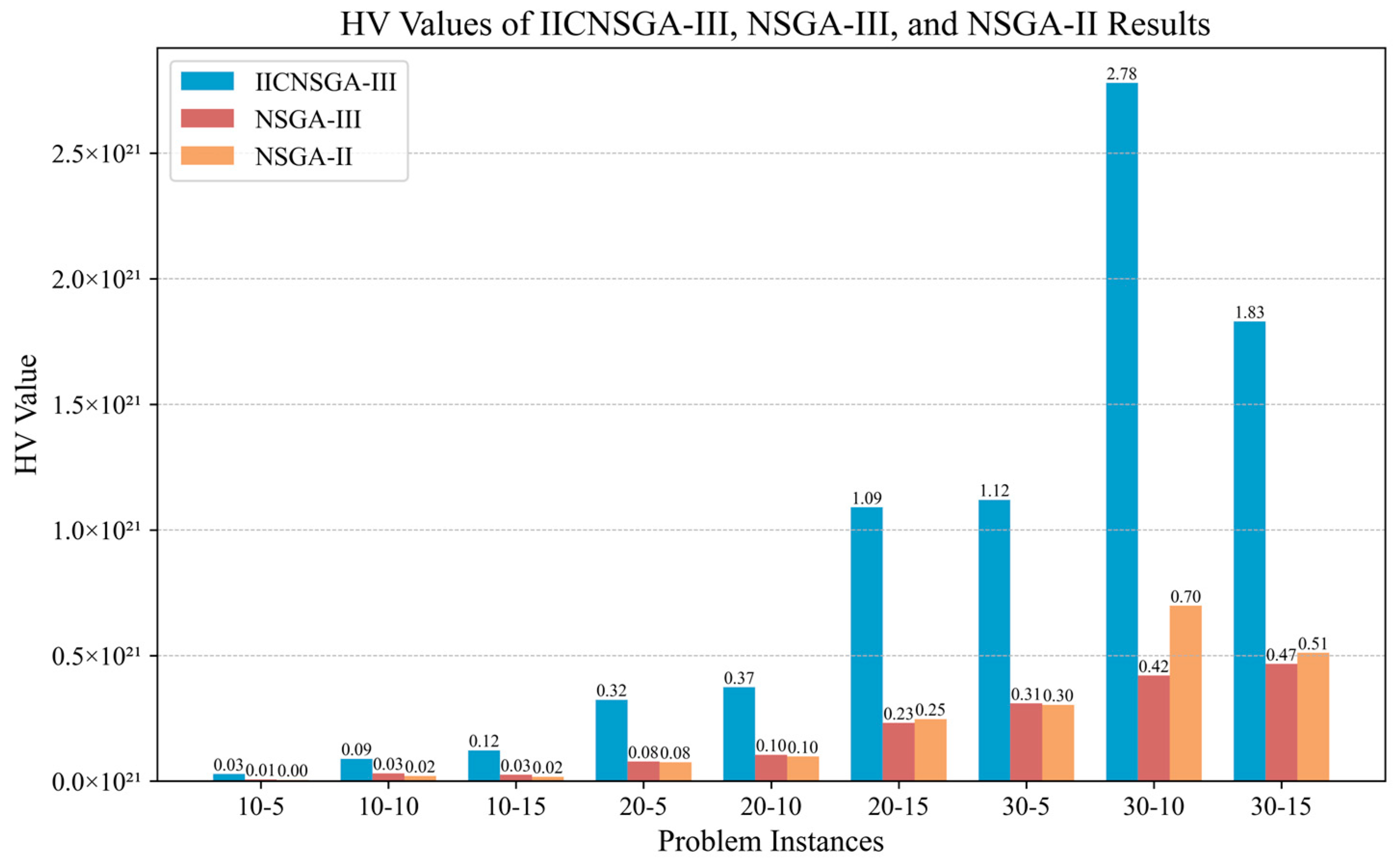
To further analyze the performance of the three algorithms across different scales, the Hypervolume (HV) indicator and the Inverted Generational Distance (IGD) are employed. The IGD value represents the volume of the region in the objective space formed by the non-dominated solution set obtained by the algorithm and the reference point. The IGD value is used to measure the discrepancy between the obtained solution set and the true Pareto front. Thus, a higher HV value and a lower IGD value indicate better overall algorithmic performance. The reference point for the HV calculation is set to a point slightly larger than all objective values, while the Pareto reference front for the IGD calculation consists of the optimal solutions for each objective function. The HV and IGD values for IICNSGA-III, NSGA-III, and NSGA-II across the nine test cases are shown in Figure 4 and Figure 5. As illustrated in Figure 4 and Figure 5, IICNSGA-III exhibits significantly superior performance over both NSGA-III and NSGA-II across the nine test cases of varying scales.
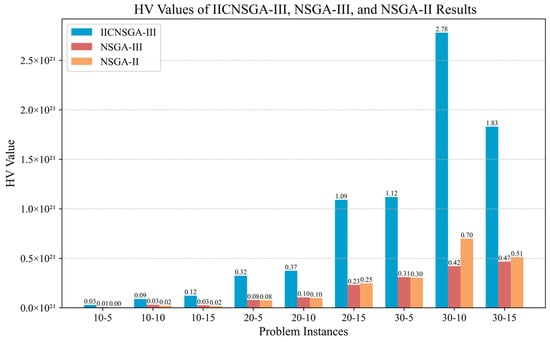
Figure 4.
Hypervolume (HV) comparison of solution sets for IICNSGA-III, NSGA-III, and NSGA-II.
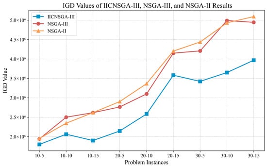
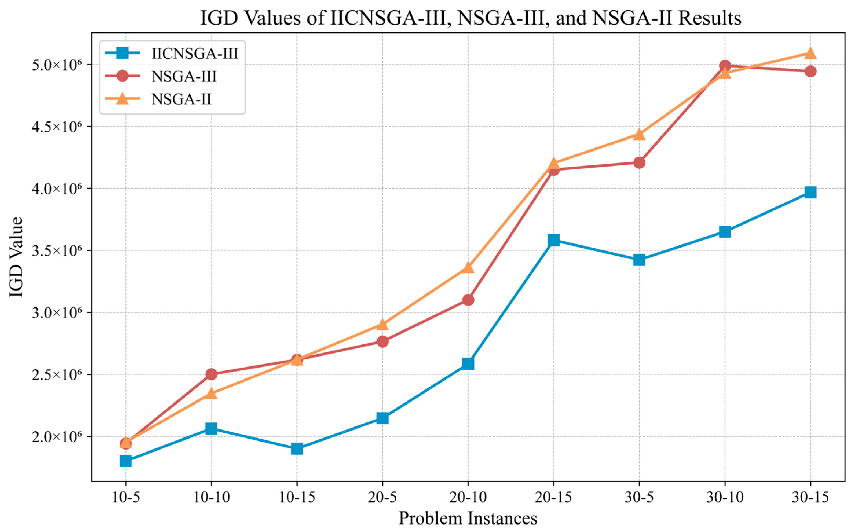
Figure 5.
Inverted generational distance (IGD) comparison of solution sets for IICNSGA-III, NSGA-III, and NSGA-II.
All HV values are expressed in units of . As shown in Figure 4, IICNSGA-III consistently achieves the highest HV values across all problem instances, with its advantage becoming more pronounced as the problem scale increases. In small-scale problems such as 10-5, IICNSGA-III reaches 0.03, three times higher than NSGA-III at 0.01. In 10-10, IICNSGA-III increases to 0.09, while NSGA-III and NSGA-II achieve only 0.03 and 0.02, respectively. The performance gap remains moderate in this range, but IICNSGA-III maintains a consistent lead.
As the problem size increases, IICNSGA-III demonstrates a stronger advantage. In 20-15, its HV value rises to 1.09, significantly outperforming NSGA-III at 0.23 and NSGA-II at 0.25. The trend becomes even more pronounced in large-scale problems. In 30-10, IICNSGA-III reaches 2.78, surpassing NSGA-III by more than six times, as NSGA-III records 0.42, and exceeding NSGA-II, which reaches 0.70. Similarly, in 30-15, IICNSGA-III achieves 1.83, far ahead of NSGA-III at 0.47 and NSGA-II at 0.51.
All IGD values are expressed in units of . As shown in Figure 5, IICNSGA-III consistently achieves the lowest IGD values across all problem instances, indicating superior convergence towards the true Pareto front. In small-scale problems, IICNSGA-III achieves 1.80 in 10-5, which is lower than NSGA-III at 1.94 and NSGA-II at 1.95. In 10-10, IICNSGA-III maintains a lower IGD at 2.06, while NSGA-III and NSGA-II record 2.50 and 2.35, respectively.
As the problem scale increases, the performance gap widens. In 20-15, IICNSGA-III achieves 3.58, significantly lower than NSGA-III at 4.15 and NSGA-II at 4.20. The trend continues in 30-10, where IICNSGA-III reaches 3.65, outperforming NSGA-III at 4.98 and NSGA-II at 4.93. For large-scale problems, IICNSGA-III demonstrates the most substantial improvement. In 30-15, it maintains the lowest IGD value at 3.97, while NSGA-III and NSGA-II record 4.94 and 5.09, respectively.
The HV and IGD metrics evaluate multi-objective optimization performance. HV provides a broad set of trade-off solutions, helping decision-makers balance conflicting objectives such as cost reduction and carbon emission control. In high-dimensional optimization with four or more objectives, traditional algorithms often fail to explore the objective space effectively. IGD measures the discrepancy between the obtained solution set and the true Pareto front, where a lower value indicates better convergence and a more reliable solution set. Reducing IGD prevents premature convergence and enhances global search. IICNSGA-III improves both HV and IGD, offering a well-distributed solution set with superior convergence. Through enhanced global search strategies, it generates solutions closer to the global optimum, supporting more precise decision-making under complex constraints.
NSGA-III and NSGA-II perform poorly in large-scale problems, especially as the number of suppliers increases. The HV value increases slightly, while the IGD value rises rapidly, indicating a tendency for early convergence and difficulty in finding the global optimum. IICNSGA-III shows clear advantages in accuracy and solution quality, particularly on complex datasets. It offers decision-makers more trade-off options among multiple objectives. The algorithm also performs well in high-dimensional optimization and constraint handling, generating a broader and higher-quality Pareto front. IICNSGA-III is well suited for multi-objective optimization with four or more objectives and multi-constraint problems, particularly where high-quality trade-off solutions are needed.
4.3. Ablation Experiment
This study introduces four mechanisms: heuristic population initialization, infeasible Solution Repair, improved crossover and mutation strategies, and Pareto simulated annealing. To examine their impact on the overall algorithm’s performance, each mechanism was replaced with a traditional counterpart, resulting in four alternative algorithms. Specifically, the algorithm obtained by replacing heuristic population initialization with random population generation is referred to as non-Heuristic Population Initialization (non-HPI). The algorithm derived by modifying the infeasible solution optimization and repair mechanism to perform only basic repairs without additional optimization steps is denoted as Infeasible Solution Repair (ISR). The algorithm that replaces the improved crossover strategy with simulated binary crossover and the improved mutation strategy with polynomial mutation is termed Simulated Binary Crossover-Polynomial Mutation (SBX-PM). Finally, the algorithm obtained by removing Pareto simulated annealing is referred to as non-Pareto Simulated Annealing (non-PSA).
These four algorithms were executed 10 times across nine test cases, using procurement cost as the evaluation benchmark. The relative percentage change (RPC) in the optimal solution values was analyzed to compare the performance of these algorithms with traditional mechanisms against the proposed algorithm. The specific calculation formula is presented in Equation (13).
Here, D(X) represents the results obtained in problem instance D when the improved mechanism is replaced with the traditional mechanism. the results obtained in problem instance D when running the proposed algorithm. A larger RPC value indicates that the mechanism has a more significant impact on the algorithm’s performance, leading to better optimization of procurement costs.
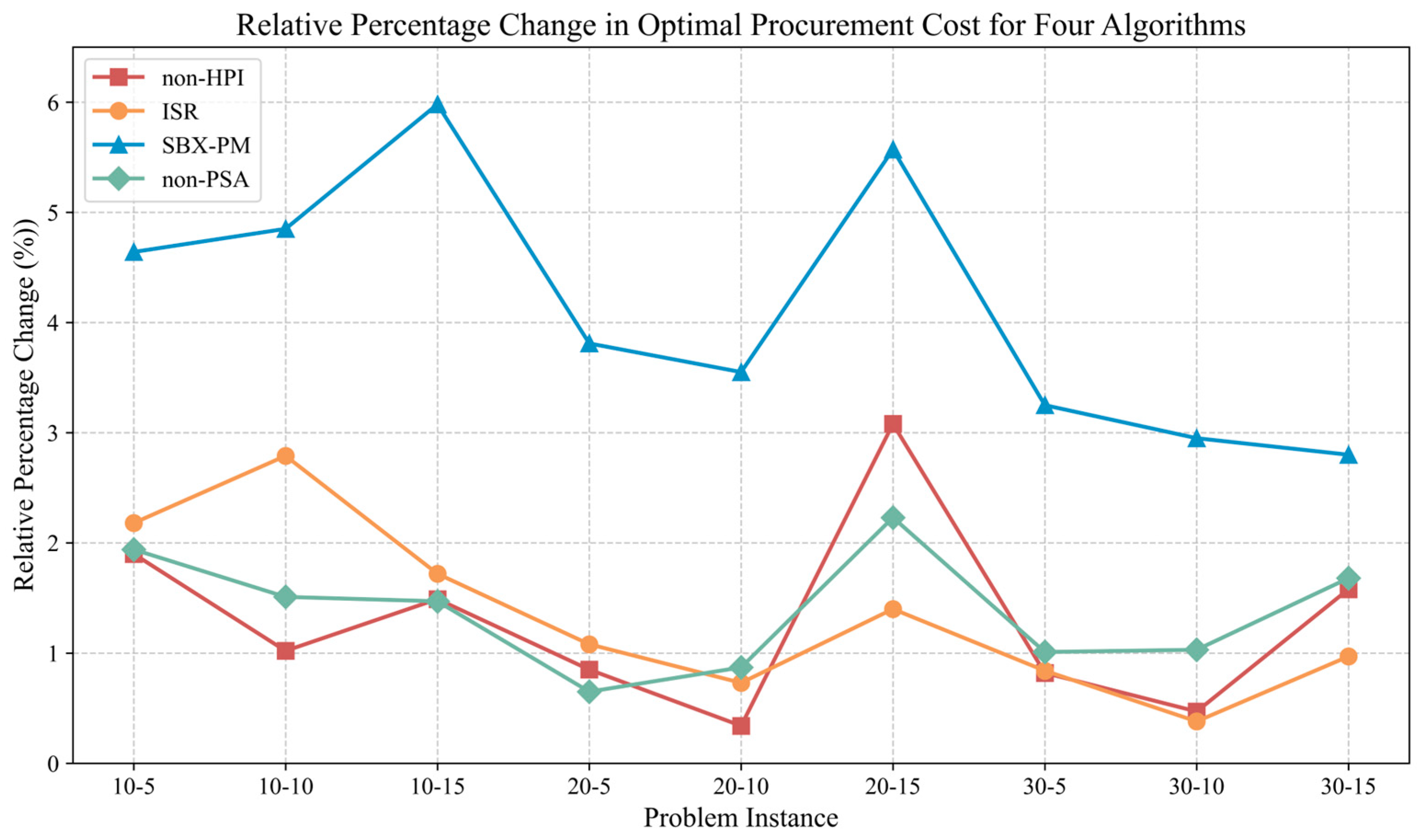
From the results in Figure 6, IICNSGA-III consistently achieves superior solutions across all problem instances compared to non-HPI, ISR, SBX-PM, and non-PSA. The improved crossover and mutation strategy performs best among the four mechanisms, achieving the highest RPC values across all test cases, with 5.98% in 10-15, 5.57% in 20-15, and 2.95% in 30-10. This indicates that the weight-matrix-based crossover operator and multi-column exchange mutation operator enhance the algorithm’s global search capability, effectively preventing premature convergence to local optima. The Pareto simulated annealing mechanism ranks second, with RPC values increasing with problem size. In 30-10 and 30-15, the values reach 1.03% and 1.68%, respectively, demonstrating that this mechanism enhances exploration and improves stability in complex optimization problems. The heuristic population initialization mechanism also demonstrates adaptability, particularly in large-scale instances. In 20-15, its RPC value reaches 3.08%, exceeding non-PSA and ISR, suggesting that a well-structured initialization strategy enables the algorithm to enter high-quality solution spaces more efficiently, improving optimization performance. The infeasible solution repair mechanism (ISR) shows relatively minor improvements but remains effective in certain cases. The RPC values are 2.79% in 10-10 and 2.18% in 10-5, indicating that repairing infeasible solutions during the search process helps reduce interference from invalid solutions and stabilizes the search direction.
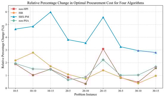
Figure 6.
Relative percentage change (RPC) in optimal procurement cost among the four algorithms.
The four improved mechanisms proposed in this study enhance the algorithm’s performance, with the crossover and mutation strategies delivering the best results.
In addition, to assess whether these four mechanisms improve the proposed algorithm’s ability to explore a broader objective space, the HV values of IICNSGA-III, non-HPI, ISR, SBX-PM, and non-PSA were calculated across nine test cases, as shown in Figure 7. Across all problem scales, the HV value of IICNSGA-III remains consistently the highest, indicating that all four mechanisms effectively enhance the algorithm’s global optimization capability.
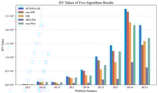
Figure 7.
Hypervolume (HV) comparison of solution sets for five algorithms.
5. Case Study
To further assess the effectiveness of the proposed approach, this study employs the 2023 procurement plan for ten products from a mechanical equipment manufacturing company as a case study to examine how to achieve more systematic and rational decision-making in supplier selection and order allocation. Currently, the company collaborates with five suppliers that can provide these ten products. Transportation-related carbon emissions constitute a significant share of the total emissions. To simplify the model and its computations, this study quantifies the total transportation-related carbon emissions from each supplier within the multi-objective optimization framework by incorporating historical average order quantities to determine the unit carbon emissions for three product categories. According to the IPCC 2006 Guidelines [34] for National Greenhouse Gas Inventories, the carbon emissions calculation formula is as follows:
The emission factor for gasoline is 2.35 kg CO2/L, with an average fuel consumption of 0.18 L per kilometer for freight vehicles. By integrating the transportation distance from each supplier to the manufacturing company along with historical average order quantities, the unit carbon emissions for each supplier, based on the ten supplied products, can be further determined. Data on material unit prices, maximum supply capacities, delivery delay rates, defect rates, delivery delay discounts, unit carbon emissions, and other relevant factors for each supplier in the case study are available in [35].
This study adopts the case company’s original order allocation strategy as the baseline and employs the proposed algorithm to solve the multi-objective optimization model, thereby adjusting the order allocation strategy. The optimized results are shown in Table 5. As shown in the table, the optimized procurement order allocation strategy derived from the proposed algorithm achieves superior performance compared to the company’s original order allocation strategy with respect to total procurement cost, total loss, total defects, and total carbon emissions.
Table 5.
Comparison of objective function values for different scenarios.
The optimized order allocation strategy reduced total procurement costs by 7.13%. This improvement resulted from reallocating product orders and prioritizing suppliers with better cost-performance ratios, ensuring more cost-effective procurement decisions. Total loss decreased to 430,588, marking a 7.58% reduction. The approach took risk factors such as delivery delays into account, favoring more reliable suppliers and mitigating operational losses associated with supply disruptions. The total number of defects also declined. Orders were reassigned based on supplier quality performance, directing them to suppliers with better historical records, which contributed to improved product quality. Carbon emissions dropped by 14.55%, demonstrating the algorithm’s effectiveness in reducing environmental impact. This was achieved by evaluating the carbon footprint of suppliers and allocating more orders to those with superior environmental performance, leading to a significant reduction in overall emissions. These findings support the company’s objective of building a sustainable and cost-efficient supply chain. The improved allocation strategy not only optimizes financial performance but also strengthens supply chain resilience and environmental responsibility.
6. Conclusions
This study presents an improved integer-coded NSGA-III algorithm (IICNSGA-III) to tackle the supplier selection and order allocation problem within the mechanical manufacturing sector, while accounting for supply chain disruption risks and carbon emissions. The model integrates traditional objectives such as procurement cost and quality with additional factors such as supplier delivery delay risks and carbon emissions, by incorporating delay discount mechanisms, penalty factors, and carbon emission assessments, to offer more scientifically grounded decision support for manufacturing firms.
Comparative experimental results show that IICNSGA-III outperforms NSGA-III and NSGA-II across multiple objectives, including total procurement cost, total loss, total defects, and total carbon emissions. As the problem scale increases with more material types and suppliers, IICNSGA-III consistently achieves lower objective function bounds without significantly increasing upper bounds. This leads to a notable improvement in solution quality. The algorithm’s effective global search strategy mitigates premature convergence and yields solutions that better approximate the global optimum.
In the ablation study, all four mechanisms—heuristic population initialization, infeasible solution optimization and repair, improved crossover and mutation strategies, and Pareto simulated annealing—significantly enhance the algorithm’s performance. Among these, the improved crossover and mutation strategies notably strengthen the global search ability, validating the importance of these mechanisms in improving solution quality and achieving multi-objective optimization.
The practical case study further demonstrates the effectiveness of the proposed model and algorithm. In the case of a mechanical manufacturing company’s procurement plan, the optimized order allocation strategy reduced total procurement costs by 7.13%, total losses by 7.58%, and total carbon emissions by 14.55%, while also decreasing the number of defects. These results indicate that the algorithm excels in reducing costs, improving quality, and achieving environmental sustainability, thereby providing strong support for green supply chain objectives.
In summary, IICNSGA-III excels in high-dimensional multi-objective optimization, complex constraint handling, and green supply chain optimization, making it particularly suitable for complex multi-objective optimization problems with multiple constraints. By balancing multiple conflicting goals, such as cost reduction and carbon minimization, the algorithm provides decision-makers with higher-quality and more adaptable trade-off solutions, substantially improving economic efficiency, environmental sustainability, and overall supply chain stability. Future research can focus on the complexity of supply chain optimization, intelligent algorithm enhancements, and green sustainability objectives. Through dynamic modeling, intelligent optimization, and industry expansion, IICNSGA-III can further improve its applicability in high-dimensional multi-objective optimization, complex constraint handling, and green supply chain management, providing more robust decision support for supply chain optimization.
Author Contributions
Conceptualization, J.Z.; Validation, M.S.; Writing—original draft, M.S.; Writing—review and editing, M.S.; Supervision, J.Z. All authors have read and agreed to the published version of the manuscript.
Funding
This research received no external funding.
Institutional Review Board Statement
Not applicable.
Informed Consent Statement
Not applicable.
Data Availability Statement
The raw data supporting the conclusions of this article will be made available by the authors on request.
Conflicts of Interest
The authors declare no conflicts of interest.
References
- Fu, Q.; Lee, C.Y.; Teo, C.P. Procurement management using option contracts: Random spot price and the portfolio effect. IIE Trans. 2010, 42, 793–811. [Google Scholar] [CrossRef]
- Chaturvedi, A.; Martínez-De-Albéniz, V. Optimal procurement design in the presence of supply risk. Manuf. Serv. Oper. Manag. 2011, 13, 227–243. [Google Scholar] [CrossRef]
- Lee, C.Y.; Chien, C.F. Stochastic programming for vendor portfolio selection and order allocation under delivery uncertainty. OR Spectrum 2014, 36, 761–797. [Google Scholar] [CrossRef]
- Lund, S.; Manyika, J.; Woetzel, J.; Barriball, E.; Krishnan, M.; Alicke, K.; Birshan, M.; George, K.; Smit, S.; Swan, D.; et al. Risk, Resilience, and Rebalancing in Global Value Chains. 2020. Available online: http://dln.jaipuria.ac.in:8080/jspui/bitstream/123456789/14300/1/Risk-resilience-and-rebalancing-in-global-value-chains-full-report.pdf (accessed on 10 January 2025).
- Steinlein, A.; Grüning, C.; Weiß, D.; Li, L.; Janssen, P.; Wagner, P. EU-China Cooperation on Decarbonizing Supply Chains: Policy Brief. Adelphi Research gGmbH. 2022. Available online: https://adelphi.de/system/files/document/adelphi_2023_policy%20brief_EU_China_decarbonize_supply%20chains_CH.pdf (accessed on 10 January 2025).
- Li, C.R.; Sarker, B.R.; Cui, G.; Chen, X.L.; Luo, W.L. An optimal procurement policy for multiple consumable accessories with different lifespan distributions. Comput. Ind. Eng. 2019, 127, 143–157. [Google Scholar] [CrossRef]
- Wu, Y.; Wang, Z.; Yao, J.; Guo, H. Joint decision of order allocation and lending in the multi-supplier scenario purchase order financing. Int. Ournal Prod. Econ. 2023, 255, 108710. [Google Scholar] [CrossRef]
- Nguyen, V.H. A hierarchical heuristic algorithm for multi-objective order allocation problem subject to supply uncertainties. J. Ind. Prod. Eng. 2023, 40, 343–359. [Google Scholar] [CrossRef]
- Ali, H.; Zhang, J. A fuzzy multi-objective decision-making model for global green supplier selection and order allocation under quantity discounts. Expert Syst. Appl. 2023, 225, 120119. [Google Scholar] [CrossRef]
- Yaghin, R.G.; Darvishi, F. Order allocation and procurement transport planning in apparel supply chain: A utility-based possibilistic-flexible programming approach. Fuzzy Sets Syst. 2020, 398, 1–33. [Google Scholar] [CrossRef]
- Lin, K.-Y.; Yeng, C.-L.; Lin, Y.-K. Evaluating Order Allocation Sustainability Using a Novel Framework Involving Z-Number. Mathematics 2024, 12, 2585. [Google Scholar] [CrossRef]
- Bai, C.; Zhu, Q.; Sarkis, J. Supplier portfolio selection and order allocation under carbon neutrality: Introducing a “Cool” ing model. Comput. Ind. Eng. 2022, 170, 108335. [Google Scholar] [CrossRef]
- Homayouni, Z.; Pishvaee, M.S.; Jahani, H.; Ivanov, D. A robust-heuristic optimization approach to a green supply chain design with consideration of assorted vehicle types and carbon policies under uncertainty. Ann. Oper. Res. 2023, 324, 395–435. [Google Scholar] [CrossRef]
- Wang, Y.; Ji, X. Optimization model for low-carbon supply chain considering multi-level backup strategy under hybrid uncertainty. Appl. Math. Model. 2024, 126, 1–21. [Google Scholar] [CrossRef]
- Sriklab, S.; Yenradee, P. Consistent and sustainable supplier evaluation and order allocation: Evaluation score based model and multiple objective linear programming model. Eng. J. 2022, 26, 23–35. [Google Scholar] [CrossRef]
- Jadidi, O.; Jaber, M.Y.; Zolfaghri, S.; Pinto, R.; Firouzi, F. Dynamic pricing and lot sizing for a newsvendor problem with supplier selection, quantity discounts, and limited supply capacity. Comput. Ind. Eng. 2021, 154, 107113. [Google Scholar] [CrossRef]
- Yousefi, S.; Jahangoshai Rezaee, M.; Solimanpur, M. Supplier selection and order allocation using two-stage hybrid supply chain model and game-based order price. Oper. Res. 2021, 21, 553–588. [Google Scholar] [CrossRef]
- Di Pasquale, V.; Iannone, R.; Nenni, M.E.; Riemma, S. A model for green order quantity allocation in a collaborative supply chain. J. Clean. Prod. 2023, 396, 136476. [Google Scholar] [CrossRef]
- Mangla, S.K.; Chauhan, A.; Kundu, T.; Mardani, A. Emergency order allocation of e-medical supplies due to the disruptive events of the healthcare crisis. J. Bus. Res. 2023, 155, 113398. [Google Scholar] [CrossRef]
- Zhang, Z.; Guo, C.; Ruan, W.; Wang, W.; Zhou, P. An intelligent stochastic optimization approach for stochastic order allocation problems with high-dimensional order uncertainties. Comput. Ind. Eng. 2022, 167, 108008. [Google Scholar] [CrossRef]
- Ruiz-Vélez, A.; García, J.; Alcalá, J.; Yepes, V. Enhancing Robustness in Precast Modular Frame Optimization: Integrating NSGA-II, NSGA-III, and RVEA for Sustainable Infrastructure. Mathematics 2024, 12, 1478. [Google Scholar] [CrossRef]
- Bharadwaj, M.; Patwardhan, M.; Sharma, K. Multi-objective optimization of responsible sourcing, consumption, and production in construction supply chains: An NSGA-III approach toward achieving SDG 12. Asian J. Civ. Eng. 2025, 26, 1305–1319. [Google Scholar] [CrossRef]
- Ma, D.; Zhou, S.; Han, Y.; Ma, W.; Huang, H. Multi-objective ship weather routing method based on the improved NSGA-III algorithm. J. Ind. Inf. Integr. 2024, 38, 100570. [Google Scholar] [CrossRef]
- Cui, H.; Cao, F.; Liu, R. A multi-objective partitioning algorithm for large-scale graph based on NSGA-II. Expert Syst. Appl. 2025, 263, 125756. [Google Scholar] [CrossRef]
- Yang, M.; Zhang, B.; Shi, Z.; Li, J. A hybrid task allocation approach for multi-UAV systems with complex constraints: A market-based bidding strategy and improved NSGA-III optimization. J. Supercomput. 2025, 81, 1–33. [Google Scholar] [CrossRef]
- Li, W.; Han, D.; Gao, L.; Li, X.; Li, Y. Integrated Production and Transportation Scheduling Method in Hybrid Flow Shop. Chin. J. Mech. Eng. 2022, 35, 12. [Google Scholar] [CrossRef]
- Tang, H.; Xiao, Y.; Zhang, W.; Lei, D.; Wang, J.; Xu, T. A DQL-NSGA-III algorithm for solving the flexible job shop dynamic scheduling problem. Expert Syst. Appl. 2024, 237, 121723. [Google Scholar] [CrossRef]
- Deb, K.; Jain, H. An evolutionary many-objective optimization algorithm using reference-point-based nondominated sorting approach, part I: Solving problems with box constraints. IEEE Trans. Evol. Comput. 2013, 18, 577–601. [Google Scholar] [CrossRef]
- Sethi, K.C.; Rathinakumar, V.; Harishankar, S.; Bhadoriya, G.; Pati, A.K. Development of discrete opposition-based NSGA-III model for optimizing trade-off between discrete time, cost, and resource in construction projects. Asian J. Civ. Eng. 2024, 25, 4633–4644. [Google Scholar] [CrossRef]
- Zhang, H.; Wang, G.G.; Dong, J.; Gandomi, A.H. Improved NSGA-III with second-order difference random strategy for dynamic multi-objective optimization. Processes 2021, 9, 911. [Google Scholar] [CrossRef]
- Zhang, J.; Cai, J.; Zhang, H.; Chen, T. NSGA-III integrating eliminating strategy and dynamic constraint relaxation mechanism to solve many-objective optimal power flow problem. Appl. Soft Comput. 2023, 146, 110612. [Google Scholar] [CrossRef]
- Shir, O.M.; Emmerich, M. Multi-Objective Mixed-Integer Quadratic Models: A Study on Mathematical Programming and Evolutionary Computation. IEEE Trans. Evol. Comput. 2024, early access. [Google Scholar] [CrossRef]
- Mirsadeghi, E.; Khodayifar, S. Hybridizing particle swarm optimization with simulated annealing and differential evolution. Clust. Comput. 2021, 24, 1135–1163. [Google Scholar] [CrossRef]
- Eggleston, H.S.; Buendia, L.; Miwa, K.; Ngara, T.; Tanabe, K. 2006 IPCC Guidelines for National Greenhouse Gas Inventories. 2006. Available online: https://www.osti.gov/etdeweb/biblio/20880391 (accessed on 17 February 2025).
- Mendeley Data, V1. Available online: https://data.mendeley.com/datasets/dsht25fbtb/1 (accessed on 17 February 2025).

Disclaimer/Publisher’s Note: The statements, opinions and data contained in all publications are solely those of the individual author(s) and contributor(s) and not of MDPI and/or the editor(s). MDPI and/or the editor(s) disclaim responsibility for any injury to people or property resulting from any ideas, methods, instructions or products referred to in the content. |
© 2025 by the authors. Licensee MDPI, Basel, Switzerland. This article is an open access article distributed under the terms and conditions of the Creative Commons Attribution (CC BY) license (https://creativecommons.org/licenses/by/4.0/).