Abstract
To enhance road safety and optimize intelligent driving systems, this study introduces the concept of “driving style tendency” to characterize short-term driver behavior, particularly lane-changing patterns. A multidimensional framework is established to analyze driving roles and behaviors, utilizing a Hidden Semi-Markov Model and Hierarchical Dirichlet Process for the unsupervised segmentation of driving trajectory data into behavioral primitives. By systematically analyzing driver behaviors in leading and following scenarios, characteristic thresholds are derived through distribution fitting, enabling the development of a non-parametric Bayesian-based scoring method for driving style tendency. The K-means clustering algorithm is employed to transform primitive segments into quantifiable semantic information, facilitating the interpretation of driver behavior preferences. This research contributes to improved collision risk prediction in complex traffic environments, supports the design of personalized driving assistance systems, and provides valuable insights for autonomous driving technology development.
1. Introduction
Lane-changing represents a complex interactive behavior that is significantly influenced by the driving styles of involved drivers. During the brief temporal window of lane-changing interactions, driving styles exhibit dynamic fluctuations due to multiple factors, including environmental conditions and driver emotional states. Hazardous lane-changing maneuvers often intensify vehicle interactions, generate traffic flow turbulence, and elevate collision risks [1,2,3,4]. The lane-changing process is characterized by velocity variations and necessitates sustained driver attention for effective interaction with surrounding vehicles, yet over 50% of lane-changing maneuvers are executed without turn signal usage [5]. Consequently, accurate identification and semantic quantification of short-term driving styles during lane-changing can enhance risk assessment precision. Driving style is influenced by multiple determinants, including the driver’s psychological and physiological states, operational skills, road conditions, and traffic flow characteristics [6,7,8,9,10]. Research in this domain primarily aims to enhance driving safety, comfort, and energy efficiency [11]. Methodological approaches to driving style investigation encompass questionnaire surveys, expert subjective evaluations, and objective behavioral analysis. Reason et al. [12] pioneered the development of driving behavior questionnaires for quantifying driver errors and violations, though these instruments lacked specific driving style metrics. Ishibashi et al. [13] subsequently designed specialized questionnaires for driving style analysis. Taubman et al. [14] introduced a multidimensional driving style inventory that precisely categorizes driving style typologies and structures, which has gained widespread adoption. Sun et al. [15] systematically reviewed driving style research and advocated for the localization of driving style inventories, subsequently implementing preliminary revisions and applications. Huang et al. [16] developed a multidimensional driving style scale and employed snowball sampling with K-means clustering to classify driving styles into aggressive, normal, and cautious categories.
While questionnaire-based analysis offers advantages in cost-effectiveness, simplicity, and data accessibility, this methodology is inherently limited by its reliance on subjective judgments from both questionnaire designers and respondents. In existing subjective research paradigms, driving styles are predominantly characterized through qualitative classifications that indicate behavioral consistency across driver populations. For instance, qualitative descriptive methods are typically employed to characterize aggressive driving styles based on observable driving behaviors. Totkova et al. [17] found that anxiety, sensation seeking, driving anger, and aggressive and risky driving behavior significantly predict compliance with traffic rules. Eboli et al. [18] established a more reliable definition of driving style through the analysis of velocity and longitudinal and lateral acceleration parameters, integrating both objective and subjective assessments to determine automobile drivers’ accident risk levels. Hajiseyedjavadi et al. [19] conducted a driving simulator study to investigate real-time subjective feedback from individuals, utilizing button-press responses to evaluate their perceptions of various autonomous vehicle driving styles. However, the unidirectional nature of qualitative description methods relying on subjective settings limits their capacity to characterize multiple driving factors accurately. Furthermore, precise estimation of driver performance in specific maneuvers based on driving style remains challenging. While subjective measurements exhibit inter-individual variability and high instability, objective methods strive to approximate factual conditions as closely as possible. Objective methodologies primarily focus on vehicle dynamic characteristics, which are directly influenced by driver behavior. Distinct driving styles manifest in measurable differences in vehicle dynamics [20,21,22,23], with recent advancements incorporating machine learning and neural network algorithms for driving style analysis [24,25,26,27]. Nevertheless, existing research frequently overlooks the dynamic nature of driving style variations and the interactive aspects between lane-changing vehicles and surrounding traffic. The application of subjective research and analytical methods to real-time scenarios continues to present significant challenges. In practice, driving styles may be influenced by diverse traffic scenario characteristics, with drivers potentially exhibiting varying behaviors and making different operational decisions under distinct risk conditions [28]. For instance, aggressive drivers may frequently execute lane changes to overtake slower front vehicles while maintaining their lane position when front vehicles operate at normal speeds with adequate spacing. The extraction of large-scale short-term lane-changing characteristic segments and the development of standardized driving style evaluation metrics, coupled with the identification of complex vehicle operations in specific scenarios, remain unachieved in current research. The investigation and quantitative assessment of short-term driving styles hold significant implications for optimizing scenario-specific management, enhancing risk prediction, and improving traffic services.
It can be seen that the traditional driving style research mainly relies on the subjective questionnaire method, which makes it difficult to capture the dynamic characteristics of short-term interactive behavior and does not achieve the coupling analysis of short-term behavior and real-time scene, while the neural network method relies on the “black box” model to output the style label, and lacks the explanation of scoring logic. This study utilizes extensive naturalistic driving trajectory data to design corresponding feature index groups for different driving roles surrounding target vehicles. Driving states are extracted from primitive segments based on time-series characteristics of lane-changing trajectories, with classification thresholds for feature indices established through distribution fitting. The integration of non-parametric Bayesian algorithms and K-means clustering enables the assignment of specific semantic information to characteristic primitive segments, ultimately achieving quantitative scoring of driving style tendencies. Major contributions include:
① The HSMM-HDP fusion framework is proposed to extract short-term driving behavior primitives from sequential trajectory data unsupervised, which overcomes the dependence of traditional methods on fixed time windows.
② A semantic mapping mechanism based on K-means clustering is designed to map feature primitive segments into interpretable semantic units, which makes up for the defect of existing semantic fuzziness of tags.
③ Through the unsupervised clustering results of feature primitives, the driving style inclination of drivers in the short-term lane-changing process is quantified, which makes the style classification more objective.
The subsequent sections are organized as follows: Section 2 presents the selection of driving style tendency characteristic indices; Section 3 details the establishment of the driving primitive segmentation model; Section 4 describes the design of the quantitative methodology for driving style tendency; Section 5 discusses conclusions and future research directions.
2. Selection of Feature Indicators
Driving style is influenced by multiple factors, including road environment, driving purpose, and driver psychology, which makes it fluctuating and complex. Previous research has also shed light on how the drivers can be classified using unsupervised methods at different locations. The results show that driver behavior will change due to changes in the surrounding environment and the personal needs of drivers [29]. Even cautious drivers may exhibit aggressive driving behavior under certain circumstances. The concept of “driving style tendency” is introduced to describe the short-term driving style of drivers [30], characterizing their driving behavior characteristics over a short period. Driving style tendency refers to the dynamic behavioral patterns exhibited by drivers in specific spatiotemporal contexts rooted in the multidimensional interaction of cognition, emotion, and environment. It is characterized by temporal dynamics, spatial interactivity, and psychological adaptability. From a psychological perspective, this concept integrates the short-term behavioral intention mechanism of the Theory of Planned Behavior, the dynamic equilibrium model of risk compensation theory, and the dual-pathway decision-making mechanism of emotional arousal, revealing the intrinsic psychological motivations behind sudden changes in driving tendencies. At the behavioral level, the stimulus-cognition-response chain model and the quantified behavioral spectrum establish a dynamic mapping between micro-level operations and environmental conditions. To assess the impact of surrounding vehicles on the target vehicle during lane changes, consider that the driving behavior of the preceding and rear vehicles has different effects on the target vehicle. For example, if the preceding vehicle suddenly decelerates or the rear vehicle suddenly accelerates, it poses a greater threat to the target vehicle [31]. Therefore, for each vehicle, distinguishing the roles of the preceding and rear vehicles and extracting their characteristic indicators is required to describe the driving style tendency.
2.1. Preceding Vehicle Driving Style Tendency Characteristics
The running characteristics of the preceding vehicle that pose a significant threat to the lane-changing behavior of the target vehicle are selected as the indicator group for driving style tendency.
- (1)
- Longitudinal Acceleration: If the preceding vehicle suddenly decelerates during a lane change, the target vehicle must brake urgently to avoid rear-end collisions. If the reaction is not timely, an accident is inevitable. Therefore, longitudinal acceleration is included in the indicator group [32].
- (2)
- Lateral Speed: If the preceding vehicle travels at a faster lateral speed, it indicates that it is pursuing high-speed travel and has generated intentions for lane changing and overtaking. The lateral stability is poor, and the lane-changing vehicle should pay attention to yielding.
- (3)
- Lateral Acceleration: Lateral acceleration reflects the rate of speed change [33]. If the lateral acceleration is too large, the vehicle is unstable laterally and prone to rollover, reflecting the urgency and impatience of the preceding vehicle driver to some extent. This is used as an indicator of the preceding vehicle’s driving style tendency.
2.2. Characteristics of Rear Vehicle Driving Style Tendency
- (1)
- Longitudinal Acceleration: The rear vehicle should decelerate to avoid the target vehicle that is in the process of lane changing. Conversely, aggressive drivers tend to accelerate to reduce the distance from the target vehicle, posing a significant threat to lane changing. Therefore, the longitudinal acceleration of the rear vehicle is used as one of the characteristic indicators.
- (2)
- Headway Distance [34]: Drivers with different styles tend to maintain different headway distances from the target vehicle. The more aggressive the style, the smaller the headway distance, which makes the driver of the target vehicle feel pressured and unable to maintain stability in the lateral direction, thus creating a greater threat.
- (3)
- Longitudinal Speed: The rear vehicle should provide sufficient space for the target vehicle to change lanes and maintain good control over its speed. Drivers adjust their speed based on the driving environment [35]. If the driver of the rear vehicle in the original lane tends to drive at high speed, it is easy to conflict with the lane-changing vehicle; if the driver of the rear vehicle in the target lane is aggressive, they may not leave enough space for the lane-changing vehicle, which can lead to lane-changing failure, causing congestion or even traffic accidents.
3. Model for Dividing Driving Baseline
The recognition of driving style tendency belongs to unsupervised classification, i.e., extracting important information from a set of sequential data to characterize the driving style and describing and distinguishing these important pieces of information. Specifically, the key features extracted in this study include longitudinal velocity and acceleration, lateral velocity and acceleration, and headway distance for both the front vehicle and the rear vehicle. By segmenting lane-changing trajectory data within a certain time window into shorter baseline segments, each segment has a different characterization significance. By combining different baseline segments, a complete lane-changing trajectory can be integrated, extracting corresponding driver behavior and style semantic information from the baseline segments to label the driving style tendency.
3.1. Hidden Markov Model (HMM)
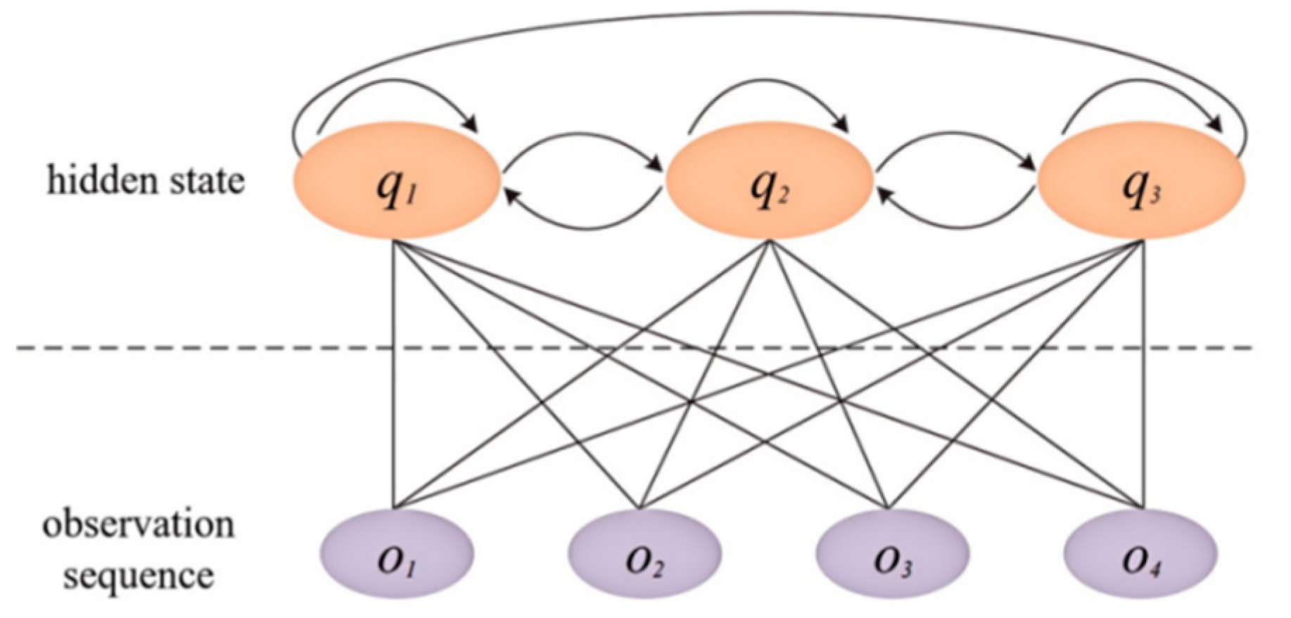
The Hidden Markov Model (HMM) is adept at handling problems where model state transitions are unobservable, states and observation sequences are not one-to-one, and belong to dynamic Bayesian network probability graph models. The model is a doubly stochastic process, divided into a random process for model state transitions and a random process for observable events under specific states. Observation variables are set as the extracted characteristic indicator group of driving style tendency. Hidden states are three types of driving behaviors, and hidden states can be inferred from observation variables [36]. At the same time, input an observation sequence into the model to obtain the mutual transformation relationship between hidden states, as shown in Figure 1.

Figure 1.
Schematic diagram of HMM structure.
Where represents the state sequence; denotes the hidden state at time i, N indicates the number of hidden states, and T represents the length of the sequence. The state at the next moment is directly influenced by the current state. O denotes the observation variable and is the corresponding observation sequence, where ot represents the observation variable at time t, and can be a combination of G variables. Typically, a Hidden Markov Model can be described by the following three key parameters: .
- (1)
- The initial state probability vector , represents the probability that the initial state of the Markov chain is si.
- (2)
- Where represents the state transition probability matrix, , indicating the probability that the Markov chain transitions from state si to state sj at time t.
- (3)
- The observation probability matrix represents the probability that the current state is si and the observation variable is Ot. where the parameter set controls the output observation probability distribution.
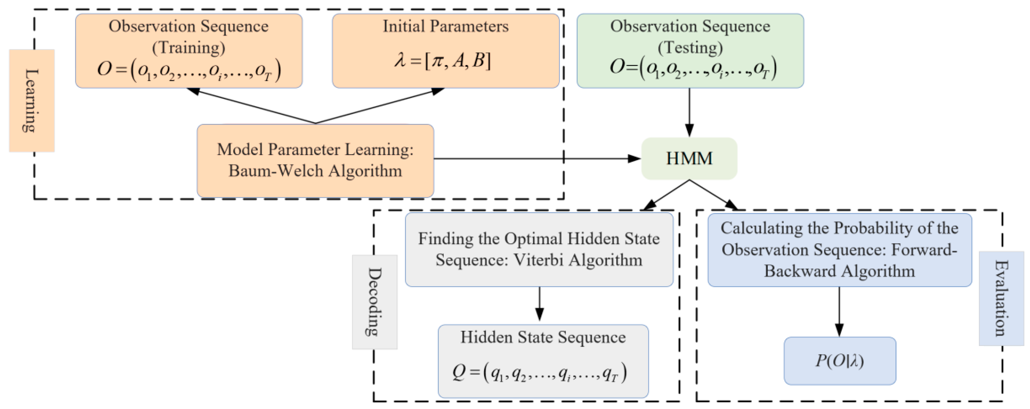
The Hidden Markov Model still needs to solve the following three problems:
- (1)
- Probability calculation problem: Given an existing Hidden Markov Model λ and a set of observation sequences, calculate P(O∣λ), which is the probability that the model λ generates the observation sequence O. This problem can be solved using forward–backward algorithms. Equations (1) and (2) define the forward and backward vectors:where is the probability that all the observation sequences O1, O2, …, Ot from time 1 to time t and the state of time t are si given the model parameter λ; is the probability of all observation sequences Ot+1, Ot+2, …, OT from time t + 1 to time T given the model parameter λ and the state of time t is si.The expression for P(O|λ) is as follows:
- (2)
- Prediction Problem: Given the model λ and an observation sequence the most likely corresponding state sequence is obtained.
- (3)
- Learning Problem: Based on known observation sequences, through training, obtain the model parameters such that the probability of the observation sequence P(O∣λ) is maximized. The relationship among these three basic problem-solving algorithms is shown in Figure 2.
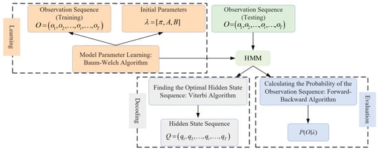 Figure 2. Schematic diagram of basic problem-solving algorithm relationships.
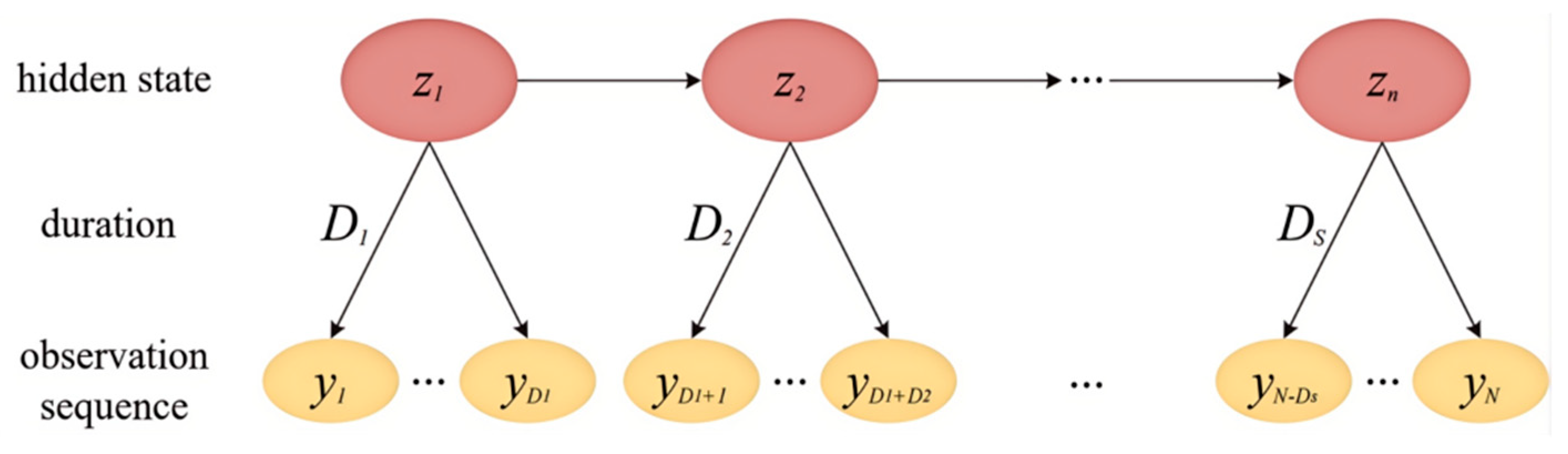
3.2. Hidden Semi-Markov Model
The hidden Semi-Markov model (HSMM) is an extension of the hidden Markov model (HMM). Unlike HMM, which generates a single observation value for each state when modeling the same time series data, HSMM generates a series of observation values for each state, forming a “one-to-many” relationship. This approach comprehensively considers the multidimensional characteristics of driving behavior. Figure 3 illustrates the structure of the HSMM model, where the new parameter D represents the duration of each hidden state. The HSMM can analyze the continuity of driving behavior. For example, during lane changing, if the target vehicle continues to be in a high lateral acceleration state, it may reflect the aggressive tendency of the driver, which is directly related to the semantic score in Section 4.4.
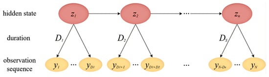
Figure 3.
HSMM model structure diagram.
HSMM model is represented by Formula (4):
where is the probability that the system is in any state at the beginning, S is the total number of states, is the probability of transition from state i to state j, and zt is the state of time t. The duration Ds of state s obeys the distribution g with parameter and yt is the generation probability of the observation value. Given the state zs and duration ds, the observation value yt follows the distribution F with the parameters and ds.
3.3. Hierarchical Dirichlet Process
Due to the inability to determine the number of hidden states in a Hidden Semi-Markov Model, the Dirichlet Process (DP) is introduced to determine the number of driving primitives. Considering the temporal characteristics of lane-changing trajectories, the feature indicators used to identify driving style tendencies are multidimensional feature sequences. A single-layer Dirichlet Process cannot meet the requirements, so the Hierarchical Dirichlet Process (HDP) is introduced. Due to the dynamic driving behavior and scene diversity, the number of driving primitives cannot be preset. HDP automatically infers the number of states (such as conservative, normal, radical, and other categories) through the non-parametric Bayesian framework, providing theoretical support for the unsupervised feature segmentation in Section 4.3.
G0 follows a DP, representing the global random measure in the measurement space Θ. Under the influence of the concentration parameter γ, its distribution quantity fluctuates within the range of the base probability measure H. The base probability measure H can also be generated by a DP.
For each group of data, each random probability measure Gj can be generated by G0 with the aid of HDP, and Gj is independent of G0, Gj distribution changes with the range of G0 distribution under the action of aggregation parameter α0.
To generate the required parameters, the gamma distribution is used as a priori. The θji factor is related to the corresponding observed variable xij:
The model structure is shown in Figure 4:
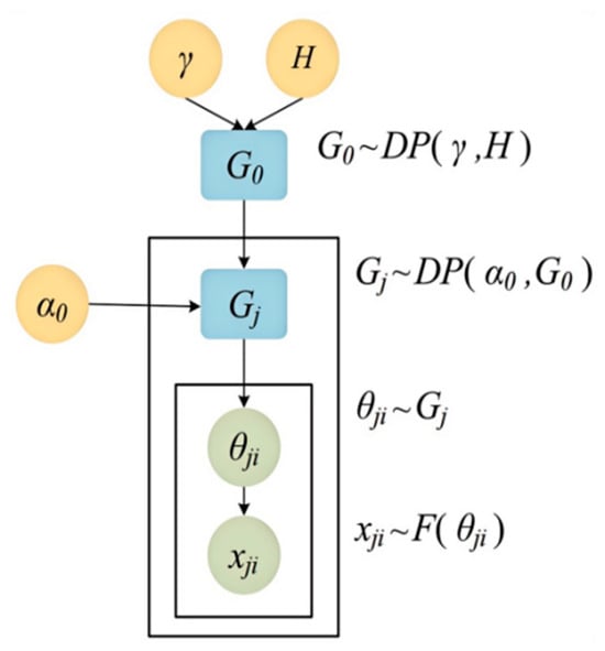
Figure 4.
Hierarchical Dirichlet process.
4. Driving Style Tendency Evaluation Based on Non-Parametric Bayesian Algorithms
4.1. Data Processing
The HighD dataset [37] is a large-scale natural driving post-processed trajectory dataset collected on German highways with no speed limit or speed limits of 120 km/h and 130 km/h in 2017 and 2018, generally consisting of four-lane and six-lane roads with a lane width of 3.75 m. A drone equipped with a high-resolution camera was used to record vehicle movement states from an aerial bird’s-eye view, providing high precision in both lateral and longitudinal directions, as shown in Figure 5. The sampling frequency was 25 Hz, and 60 trajectory data were captured at six locations, with a total duration of 16.5 h. The recorded section was approximately 420 m long, and each recording time was about 17 min. The statistical information for each location is shown in Table 1. A total of over 80,000 passenger cars and over 20,000 trucks were recorded, amounting to 110,516 vehicles, covering a distance of 44,050 km. On average, each vehicle was visible for 13.6 s, and 5600 lane-changing behaviors were captured. Each vehicle in the dataset has an average visible recording time of only 13.6 s, which falls within the scope of short-term interaction behavior research. Therefore, we select full-time domain data for the captured vehicles to study driving style tendencies.
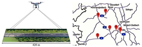
Figure 5.
HighD data set acquisition location and measurement diagram.

Table 1.
HighD dataset statistics.
To accurately describe the vehicle’s acceleration and deceleration process, we redefine the positive and negative meanings of longitudinal velocity and acceleration data according to the actual driving environment and direction. When the speed is greater than 0, the vehicle is moving forward in the driving direction. When the acceleration is greater than 0, the vehicle is in an accelerating state; when it is less than 0, it indicates that the vehicle is decelerating. We define the positive and negative meanings of lateral velocity and acceleration to make them practically meaningful. According to the driving direction, we uniformly define the positive and negative directions: a steering wheel deflection to the left of the driving direction is defined as positive, and a deflection to the right is defined as negative. Data were collected and recorded on a section of road approximately 420 m long. During this study, it was found that some headway distance values approached 400 m, which did not conform to the actual traffic environment. The headway distances in the dataset that did not match the real-world conditions were redefined. When the headway distance is less than 150 m, it is considered that the vehicle is in the following state. When the headway distance is greater than 150 m, it is considered that the vehicle is in a distant state from the preceding vehicle, and this is uniformly described as a distance of 160 m.
4.2. Threshold Division of Feature Parameters
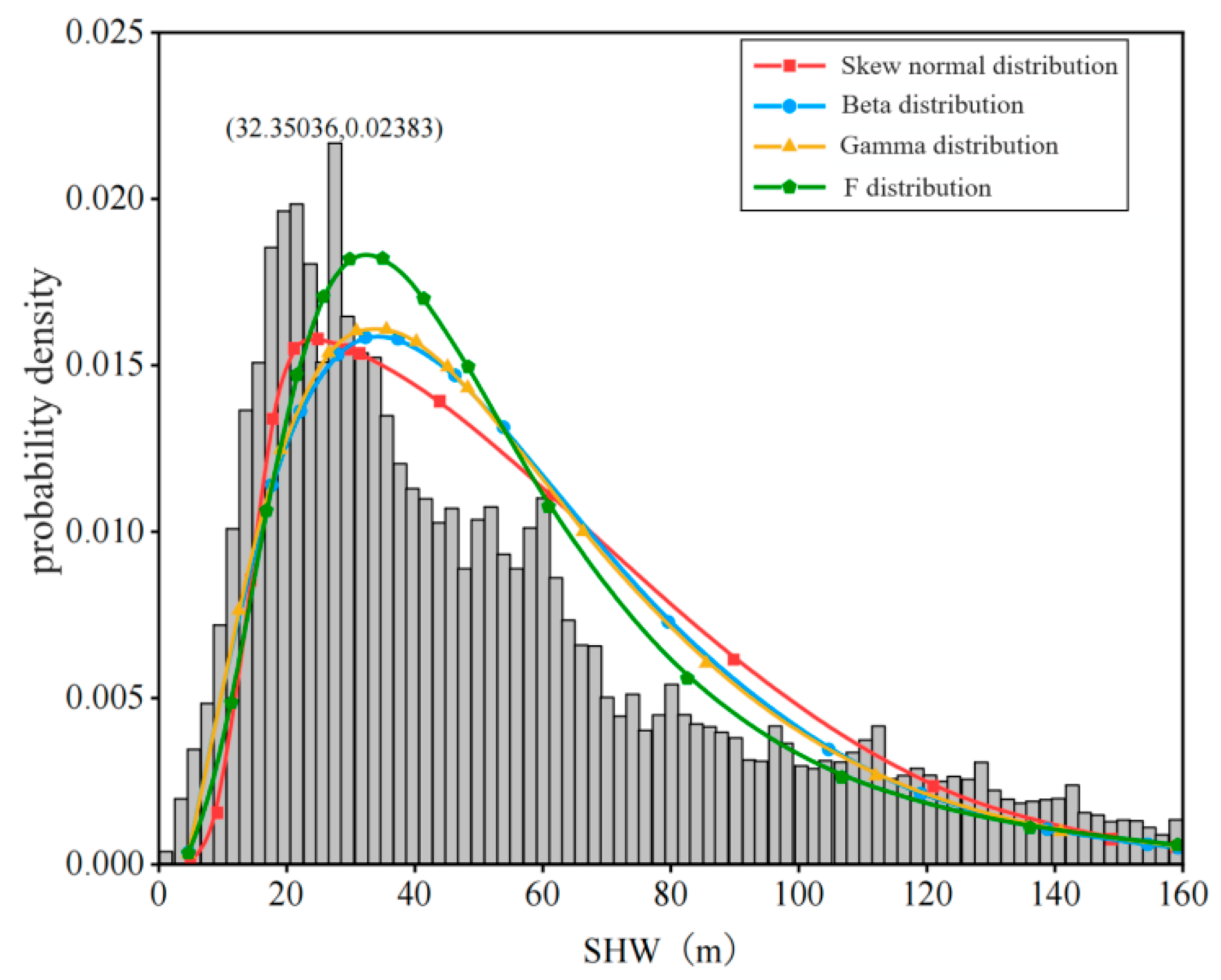
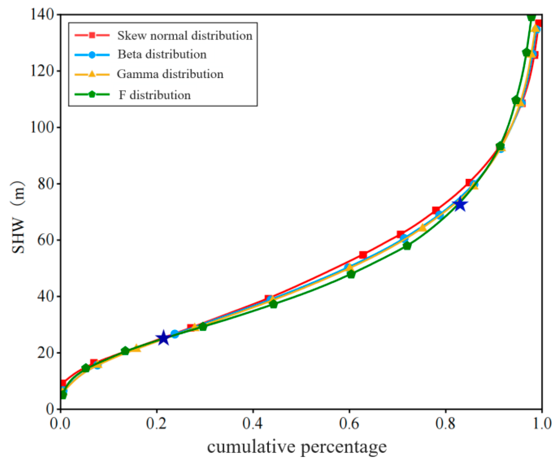
The distribution fitting of driver trajectory data, including longitudinal velocity, longitudinal acceleration, lateral velocity, lateral acceleration, and headway distance, was performed. Taking the headway distance as an example, skewed normal distribution, beta distribution, gamma distribution, and F distribution were selected to fit the headway distance for all drivers. Figure 6 shows the probability density function fitting overlaid with the histogram of these data’s distribution.
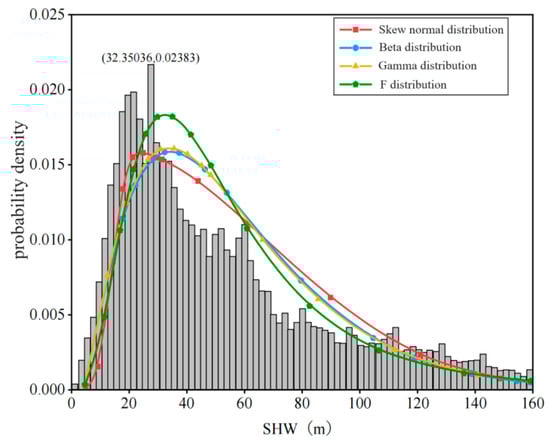
Figure 6.
Plot of fitted probability density function for space headway.
To compare the fitting effects of four distributions, the error size between sample data and the fitted distribution is used as an evaluation metric. The smaller the error, the better the fitting effect. Among them, the fitting effect error of F distribution for all drivers’ headway is the smallest, and the fitting effect is the best. Figure 7 shows the generated cumulative distribution function (CDF) plot. The parameters with the best fit are extracted: at the 25th percentile of the F distribution, the headway distance is 27.15 m; at the 85th percentile, the headway distance is 79.27 m. These two percentiles are chosen as the basis for dividing the headway distance thresholds, categorizing the headway distances into three states: long distance, medium distance, and short distance.
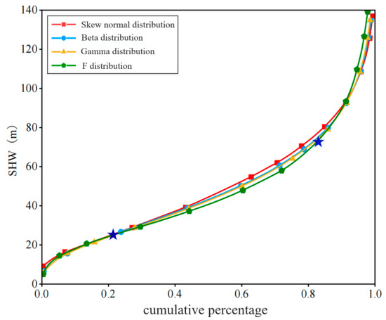
Figure 7.
Plot of cumulative distribution function.
For the remaining front and rear vehicle feature parameters, distribution fitting was also performed, and thresholds were defined based on the characteristics of the parameters. In addition to dividing the longitudinal acceleration of the front vehicle into three states, the other parameters were divided into five states based on cumulative percentages of 20%, 40%, 60%, and 80% percentiles. Through the application of distribution fitting and threshold-based partitioning, the model achieved classification accuracies exceeding 90% for longitudinal acceleration, lateral velocity, and other critical trajectory parameters. This robust performance substantiates the efficacy of the feature extraction process, demonstrating that percentile-driven state divisions effectively captured the discriminative characteristics of vehicular motion behaviors. The results of the threshold division for the front and rear vehicle features are shown in Table 2 and Table 3.
Table 2.
Front vehicle feature threshold division table.
Table 3.
Rear vehicle feature threshold division table.
4.3. Extraction of Feature Primitive Segments
Reasonably segmenting the initial driving behavior trajectory sequence is a prerequisite for subsequent research. Reorganizing and stitching adjacent samples into similar sequence blocks is an effective segmentation algorithm, provided that the adjacent samples must have the same characteristics. The boundaries of the resulting sequence blocks are referred to as sequence splits. The driving behavior features meet the above sample conditions, and HDP-HSMM was ultimately selected as the lane-changing trajectory sequence segmentation algorithm. To deeply analyze the mechanism of the quantitative model of driving style tendency, driver Y was randomly selected from the dataset. Real driving behavior data for this driver were used as the research object to systematically analyze the behavioral characteristics exhibited by the driver when acting as the front vehicle and the rear vehicle in different driving roles.
- (1)
- Feature Primitive Segments as the Front Vehicle
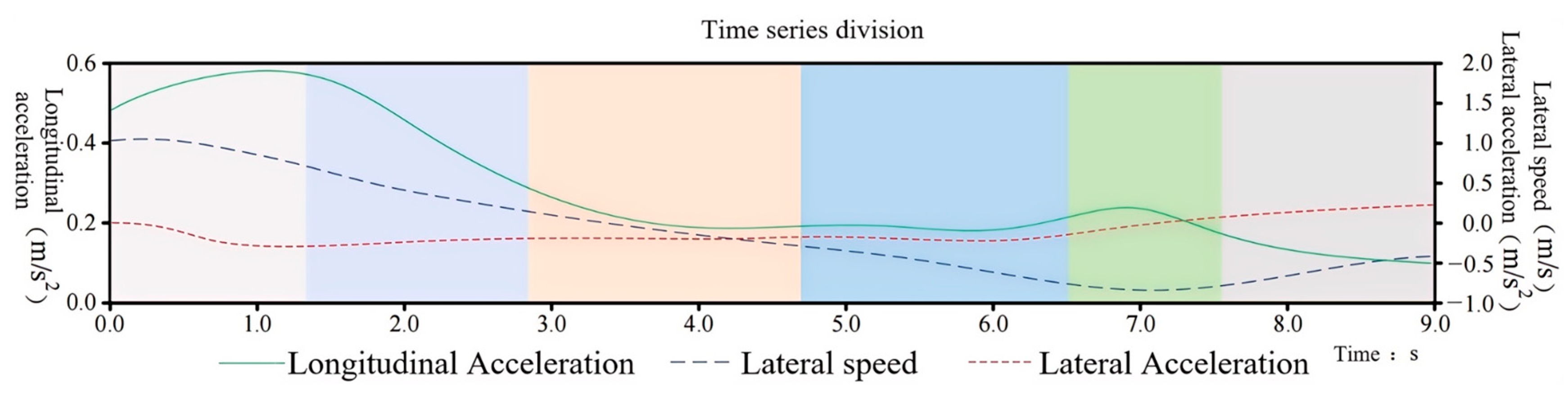
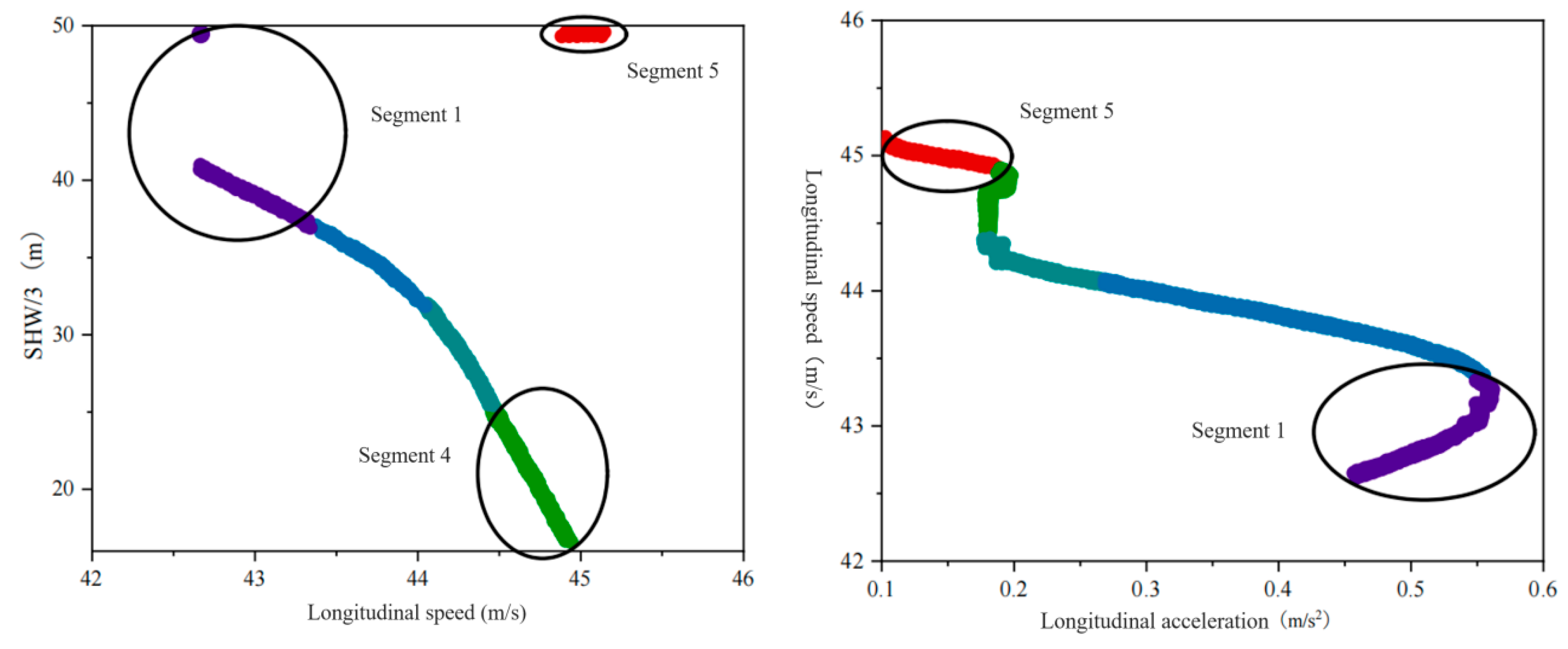
The temporal segmentation results of the trajectory characteristics of driver Y as the front vehicle can be intuitively observed in Figure 8. The numbers reflected in the coordinate system are standardized real data. Among them, the orange solid line represents the longitudinal acceleration, which shows a large variation but remains positive, indicating that driver Y is in a continuous acceleration phase; the blue long dashed line represents the lateral speed, which decreases from 1.18 m/s to −0.42 m/s, indicating that the driver initially drove to the right and then turned left; the red short dashed line represents the lateral acceleration, which originally showed a trend of accelerating to the left but changed to accelerating to the right at a certain moment, with significant fluctuations.
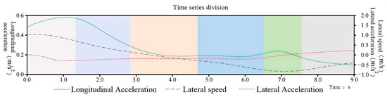
Figure 8.
Characterization data segmentation as a front vehicle.
Referring to the changes in the characteristic parameters of driver Y as the front vehicle, the HDP-HSMM segmentation algorithm automatically categorizes data with similar features into the same driving behavior. Ultimately, it divides the driving trajectory data into six driving primitive segments. Different color blocks represent different driving behaviors, with each segment having a different duration. The wider the color block, the longer the corresponding driving behavior segment lasts. The durations of the six segments are as follows: 1.24 s, 1.60 s, 1.76 s, 1.88 s, 1.12 s, and 1.36 s. Analyzing the segmentation of the trajectory time series in Figure 8. Segment 1: The longitudinal acceleration continues to increase while the lateral speed and acceleration decrease; Segment 2: The longitudinal acceleration begins to show a downward trend, with a slight recovery in lateral acceleration, and the lateral speed continues to decrease; Segment 3: The downward trend in longitudinal acceleration becomes more moderate; Segment 4: When the longitudinal acceleration remains stable, the lateral speed continues to decrease; Segment 5: The longitudinal acceleration first increases and then decreases, but with a small amplitude, and the lateral acceleration slightly increases; Segment 6: The lateral acceleration shows little change, with a tendency for the lateral speed to increase, and the longitudinal acceleration continues to decrease.
HDP-HSMM shows significant advantages in driving behavior analysis through the deep integration of the non-parametric Bayesian framework and explicit time series modeling. The algorithm successfully establishes a dynamic correlation mechanism between characteristic parameters and driving behavior. Its core is to use HDP to automatically infer the implicit state category of driving intention, avoid manual preset deviation, and explicitly model the state residence time through HSMM, accurately capture the driving primitive segment, and align it with the trajectory feature sequence to achieve space–time alignment, breaking through the limitations of the fixed time window of the traditional model. The model supports multimodal feature fusion (vehicle motion parameters, environmental perception data, and physiological signals) and is based on dynamic context-sensitive state transition mechanisms (such as cross-scene differentiated learning), which can accurately identify the subtle patterns of driver state changes. This “feature base semantic” full chain parsing ability not only achieves the mapping from micro-operation to macro-driving intention but also provides a high-precision and strong generalization algorithm basis for the anthropomorphic decision-making of automatic driving and driver risk warning, fully demonstrating its strong ability to evaluate driving behavior dynamically.
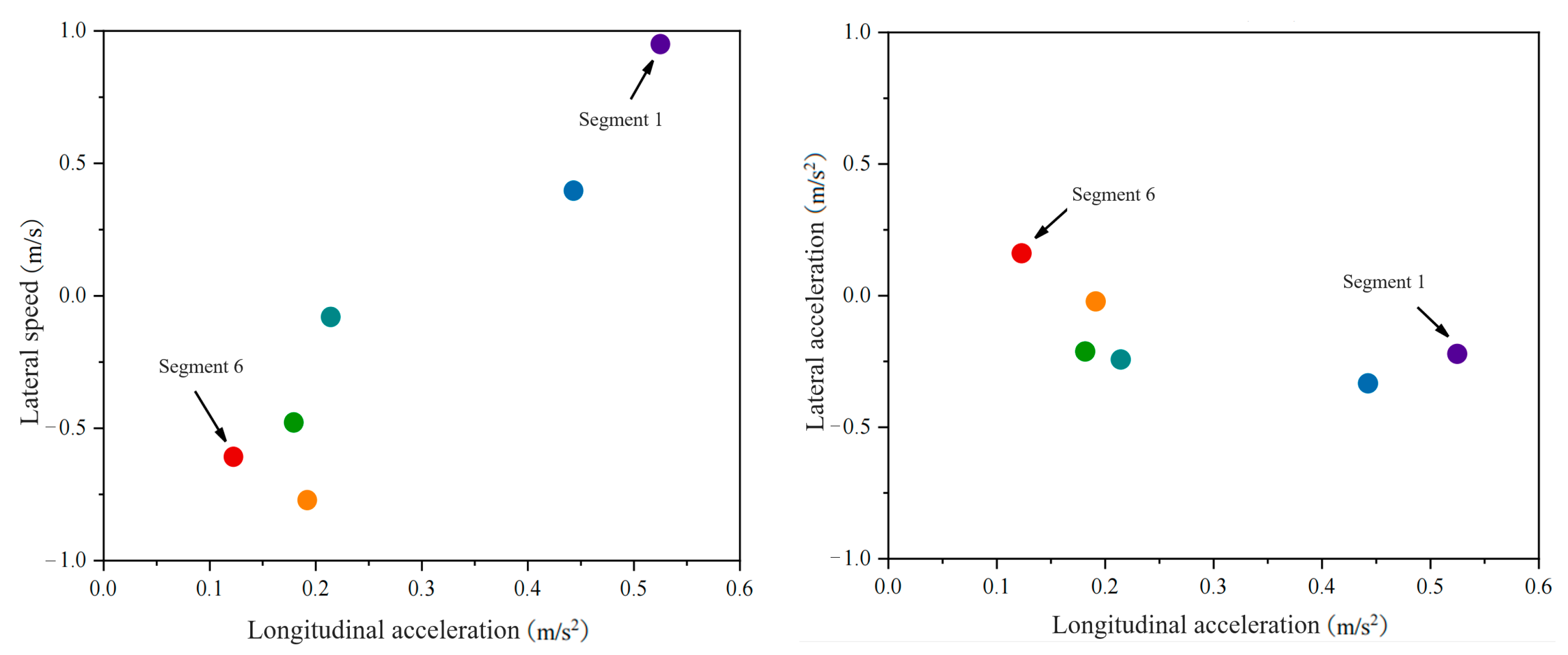
Changes in the characteristic parameters of the driving primitive segments for driver Y as the front vehicle are shown in Figure 9. The figure intuitively displays the trends of the six driving primitive segments. A group of trajectory time series data presents one segment. Starting from the effective conversion of segment information into semantic information, clustering each group of time series data, the clustered points serve as the representative attributes for the final feature markers of each segment.
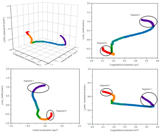
Figure 9.
Variation of the parameters of the characteristic primitive segments as a front vehicle.
- (2)
- Feature Primitive Segments as the Rear Vehicle
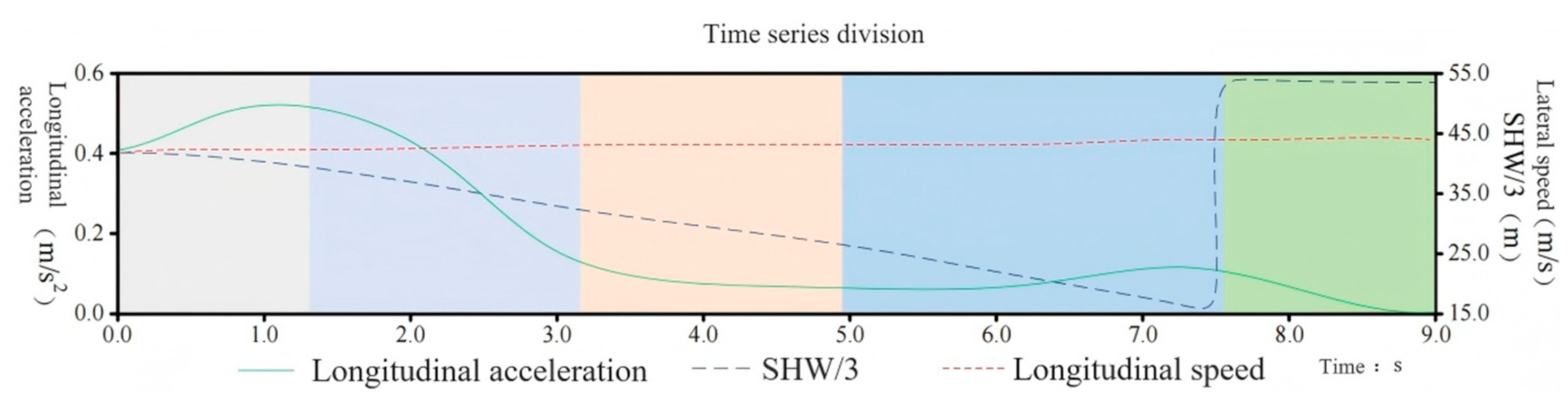
Similarly, the feature parameter time series of driver Y as the rear vehicle were segmented, with the results shown in Figure 10. The orange solid line represents the longitudinal acceleration, which is always greater than 0. The vehicle initially accelerates slightly, and the acceleration trend gradually slows down later. The green long dashed line represents the headway distance divided by three. The headway distance continuously decreases, and at around 7.4 s, the driver completes the lane change, causing a sharp increase in the headway distance. The brown short dashed line represents the longitudinal velocity, which shows a continuous slight upward trend.
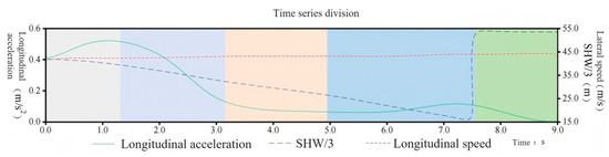
Figure 10.
Characteristic driving data segmentation as a rear vehicle.
Based on the changes in the feature parameters of the rear vehicle, the HDP-HSMM algorithm segmented driving trajectory data into five driving primitive segments. The durations of each segment are as follows: 1.36 s, 1.68 s, 1.92 s, 2.48 s, and 1.52 s. It is evident that the algorithm can identify changes in driving behavior corresponding to specific data variations, such as a decrease in longitudinal acceleration between 2 and 3 s and a sudden increase in headway distance between 7 and 8 s. This demonstrates the rationality of the time series segmentation.
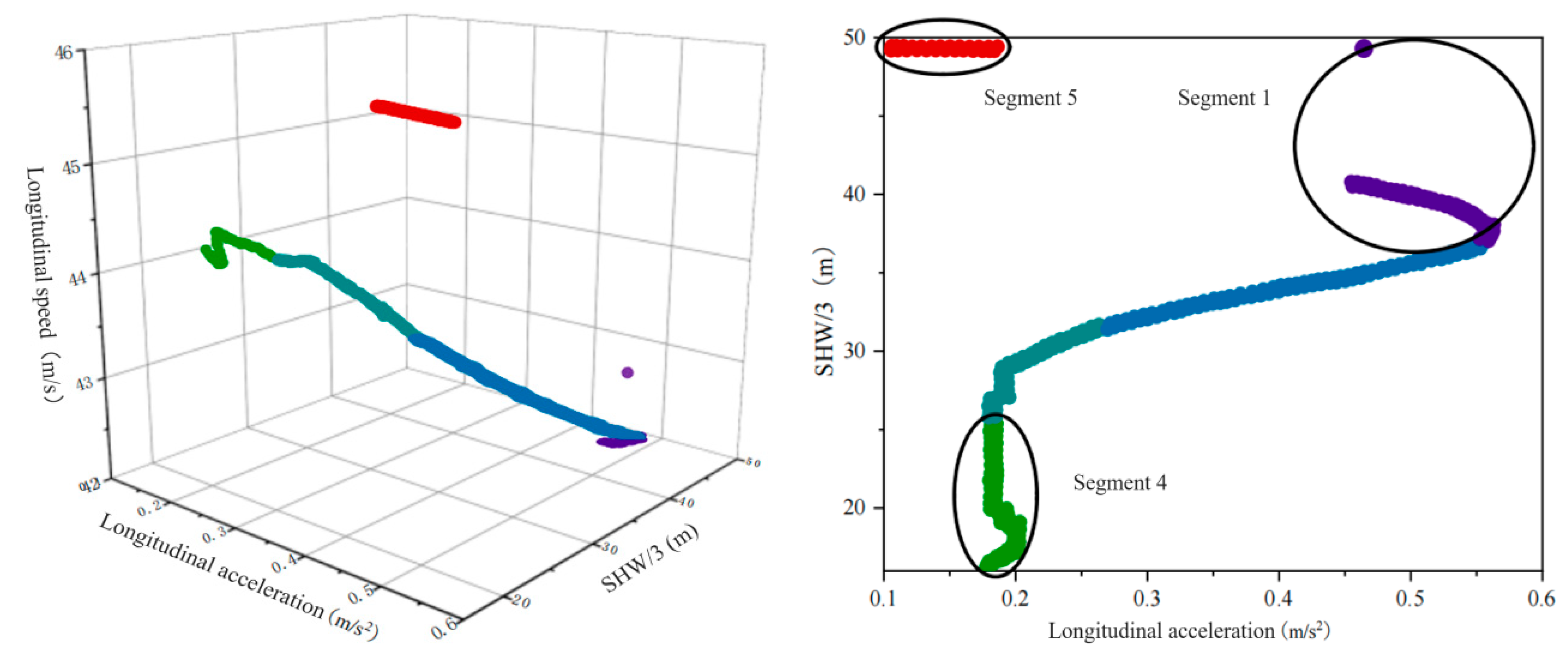
Figure 11 shows the change in the feature primitive segment parameters when driver Y is the rear vehicle. Time series data for the driving trajectory are not continuous, and there are two abrupt changes. The first mutation occurred in Segment 1. The reason is that here, the driver just completed a lane change behavior, resulting in a sudden change in headway, while only the trajectory points at 0.05 s in these original lane driving data are included in this time series. HDP-HSMM algorithm divides trajectory point and continuous state trajectory data groups after lane change into the same sequence segment through in-depth analysis of the trajectory, effectively avoiding the problem that the primitive segment is too short and showing the superiority of the algorithm in processing continuous time series data. For the second time, it appears on the sequence segmentation boundary line of Segment 4 and Segment 5. Also, because the driver changes lanes, the headway mutation occurs. The algorithm takes the state duration into account and divides trajectory data time series into Segment 4 and Segment 5. From the above analysis, the conclusion is as follows: The HDP-HSMM algorithm demonstrates temporal sensitivity and flexibility in modeling driving behavior by explicitly incorporating the duration of each behavior mode. Unlike traditional methods that often treat behavioral transitions as instantaneous events, HDP-HSMM leverages its non-parametric Bayesian framework to dynamically infer the variable persistence of driving primitives. This capability enables precise identification of mode transitions, such as the shift from cautious to aggressive driving, by accounting for both the temporal continuity and state persistence inherent in natural driving scenarios. A key innovation lies in its trajectory segmentation strategy, which integrates spatiotemporal features (e.g., longitudinal/lateral accelerations and headway distance) to group consecutive trajectory points post-lane-change into coherent segments. HDP-HSMM ensures that continuous driving modes (e.g., complete lane change maneuvers) are captured as uniform segments by avoiding the premature segmentation of trajectory data into too short intervals (common limitations of fixed windows or parameterization methods). This solves the problem of time consistency in trajectory analysis and enhances the robustness of behavior classification in a dynamic environment.

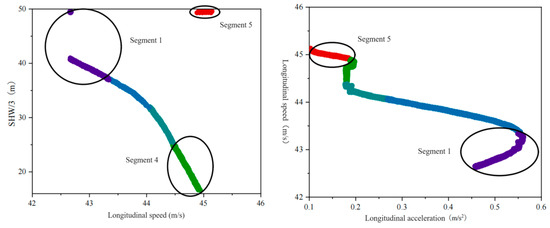
Figure 11.
Parameter variation of feature primitive segments as a rear vehicle.
4.4. Style Tendency Semantic Scoring
- (1)
- Driving Style Tendency Scoring as the Front Vehicle
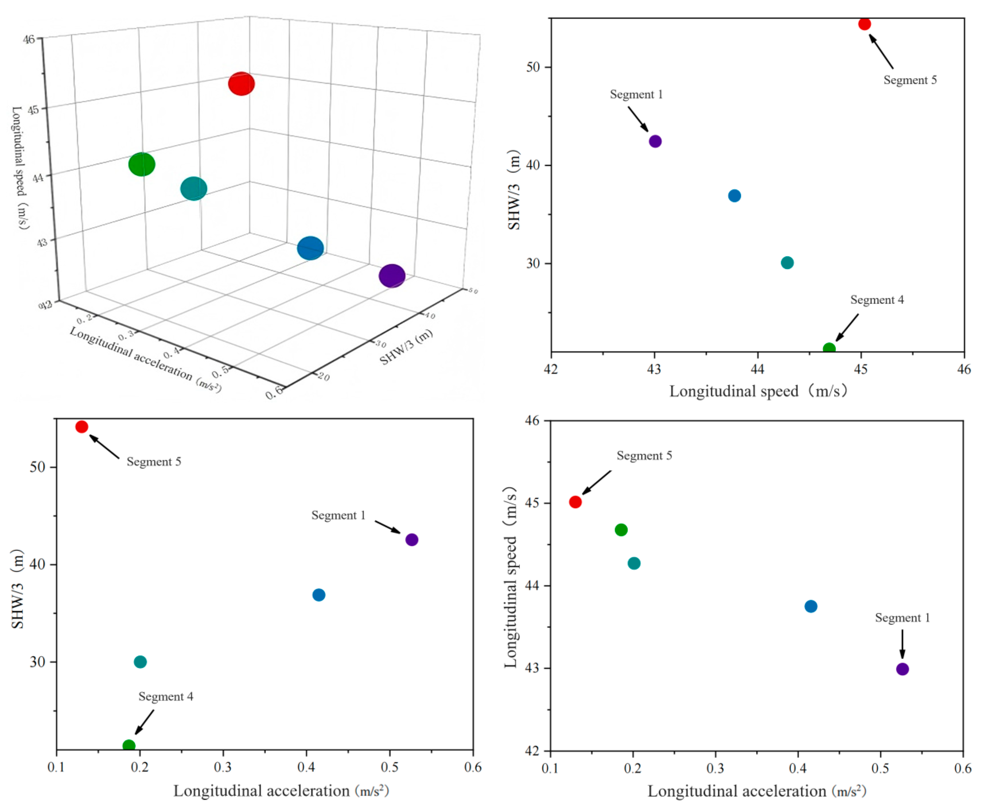
Using the K-means clustering algorithm, driving trajectory data that have been segmented into primitive segments are extended to a level where they can be converted into semantic information. After clustering, it is easier to label primitive data, enhancing interpretability. The clustering parameter k is set to 1, and all data points within each driving primitive segment are clustered into a single centroid. To eliminate the impact of the duration of the primitive segments on the clustering results, the frequency of the style semantic information represented by each driving behavior segment over a certain research period is given particular attention. The time series data clusters with driver Y as the front vehicle are classified into a single point, as shown in Figure 12.
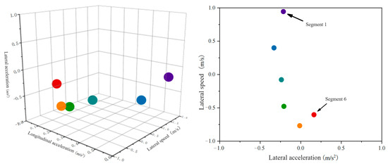

Figure 12.
Distribution of feature primitive segments after clustering as a front vehicle.
By comparing the threshold values of three types of front vehicle features in Table 2 with these aggregated point data, match the driving states with parameter values one by one to determine the driving primitive features represented by each aggregated point. Simultaneously, key descriptive feature semantics are extracted and summarized in Table 4.
Table 4.
Feature Labeling Results After Clustering of Driving Roles in the Front Vehicle.
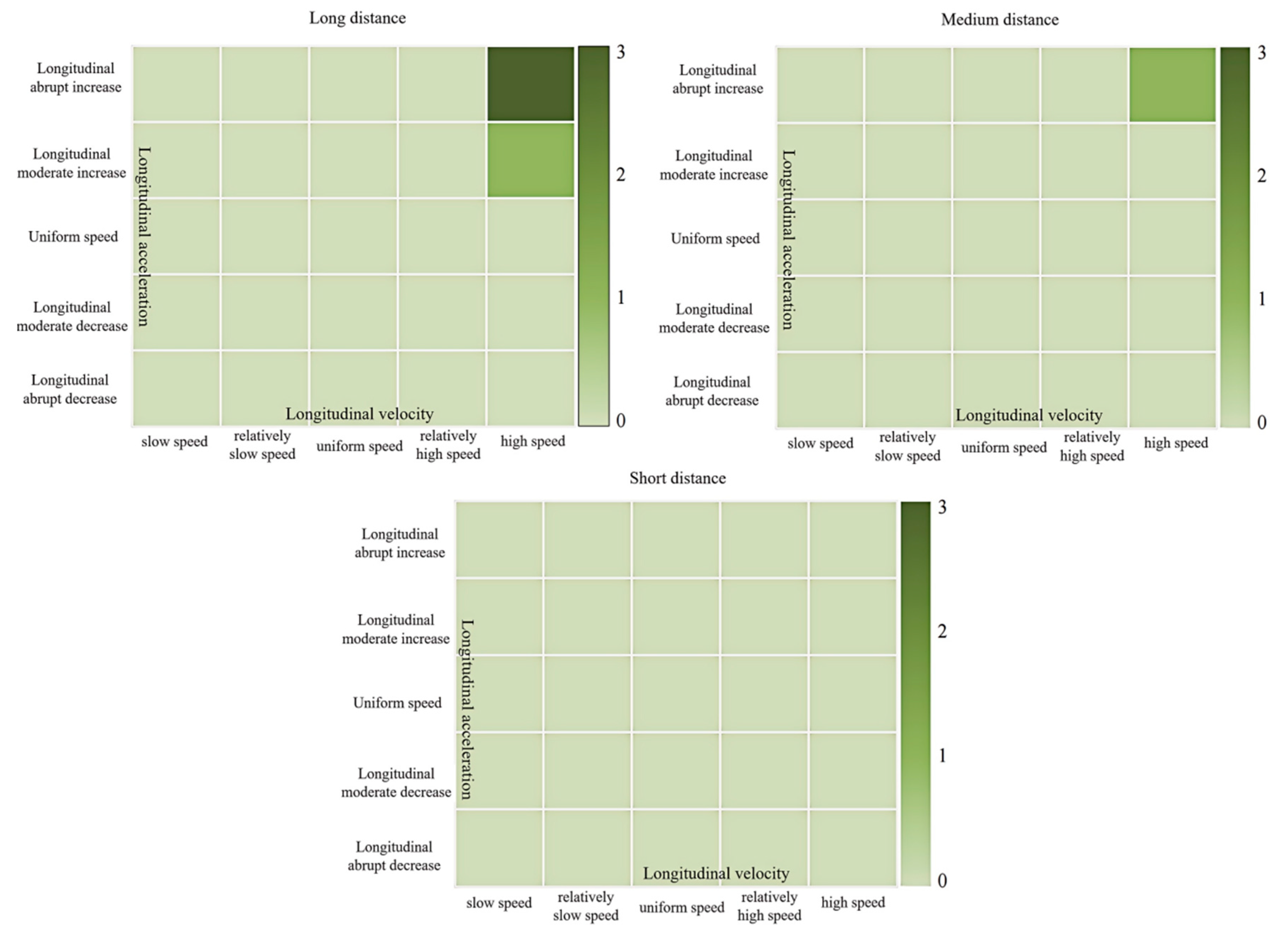
The feature values reflected by the aggregation points of characteristic primitive segments describe their corresponding driving style tendency states. The marked results are shown in Figure 13. Each figure represents a longitudinal acceleration state, with the horizontal and vertical axes representing the vehicle’s lateral velocity and acceleration, respectively. Each cell is assigned a specific driving style tendency and its corresponding semantic features. The depth of color in each cell represents the number of extracted driving behaviors.
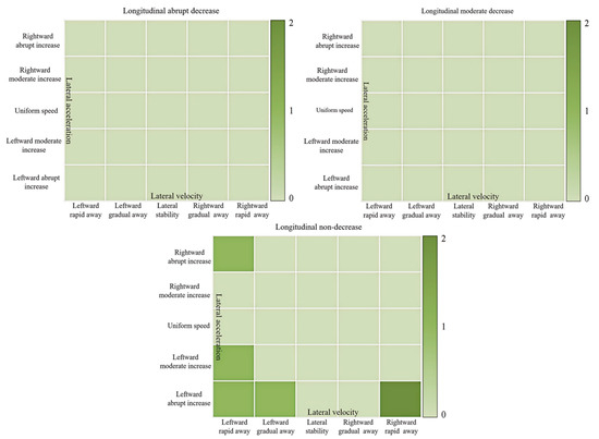
Figure 13.
Aggregate point labeling results for feature primitive fragments as front vehicles.
By observing Figure 13, it is found that all aggregation points of characteristic primitive segments are concentrated in the non-decreasing longitudinal state unit. The semantic units for abrupt and gradual decreases in longitudinal states lack corresponding driving behavior data. This means that when driver Y is the front vehicle during lane changes, there is no potential collision risk with the target vehicle in the longitudinal direction. However, the lateral states corresponding to the driving behavior primitive segments of this driver are mainly in the semantic units of “fast leftward”, “gradual leftward”, “fast rightward”, “sudden leftward acceleration”, “gradual leftward acceleration”, and “sudden rightward acceleration”. The lateral stability is poor, indicating that the driver is pursuing higher driving speed and more space through lane changes or overtaking, with a strong sense of driving urgency. This poses a threat to the target vehicle laterally. It is necessary to remind the target vehicle to observe carefully during lane changes, maintain a safe distance, and yield in time to avoid accidents.
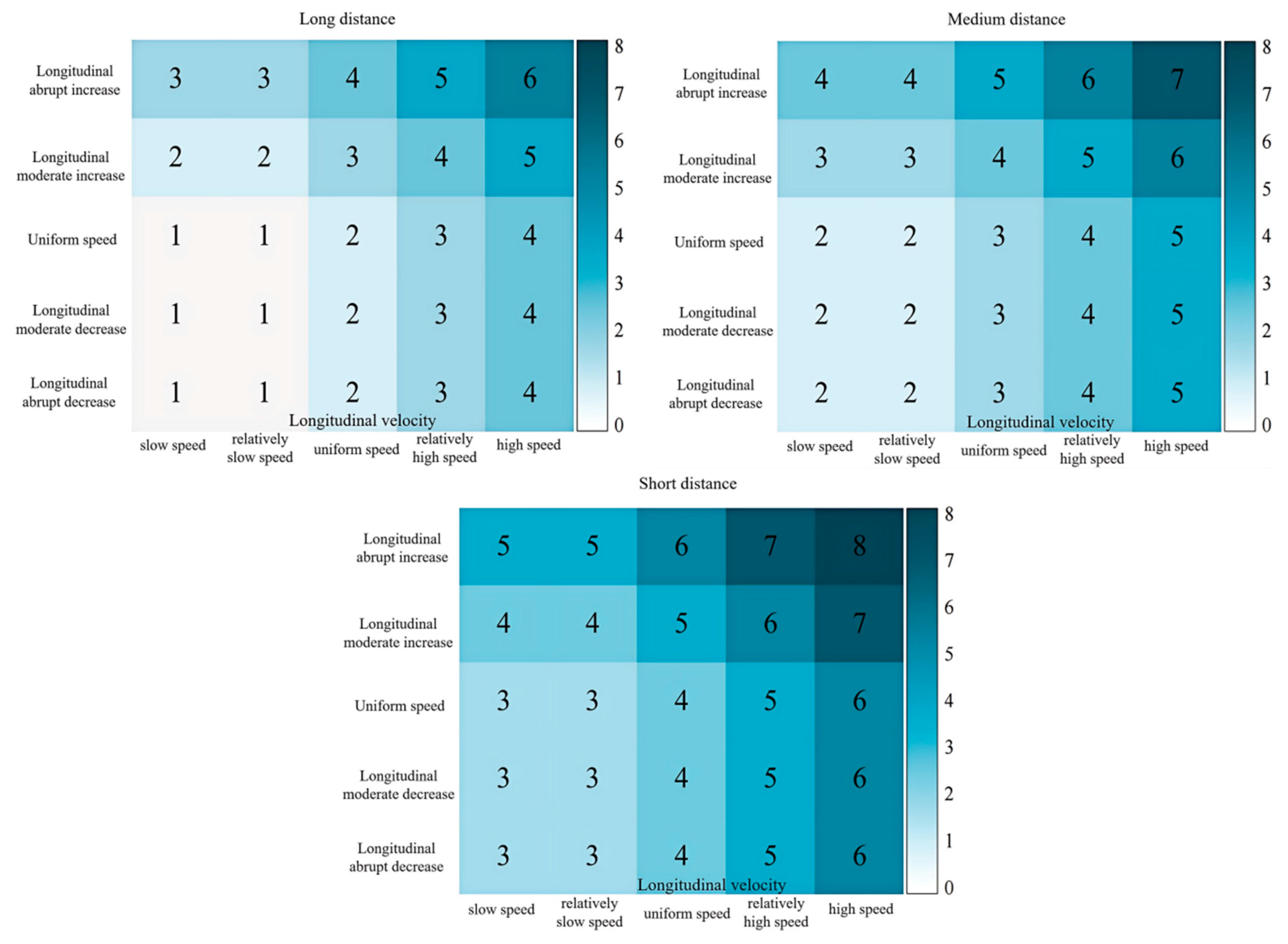
To evaluate the risk when Y is the front vehicle driver of the target vehicle, a scoring system for driving style tendencies is established. The scoring principles comprehensively consider the increase in lateral instability and changes in longitudinal acceleration that pose threats to the target vehicle. When the vehicle deviates laterally from its normal trajectory or experiences severe fluctuations in longitudinal acceleration, the potential danger to the target vehicle significantly increases. The score represents the degree of aggressiveness of the driving style of the front vehicle driver. Higher scores indicate more aggressive driving styles, posing greater threats to the safety of the target vehicle. It is considered that the combination of non-decreasing longitudinal, stable lateral, and constant lateral speed is the safest driving state, with a score set at 1. Each increment in the sub-state risk level brings the same degree of danger to the target vehicle. For example, if the lateral stability upgrades to a gradual leftward shift, the corresponding cell score increases by 1. There is a specific threshold set for determining an aggressive driving style. In this case, the threshold is set at 5.5. When the score of the front vehicle driver’s driving style tendency passes this threshold of 5.5, the driver is deemed to have an aggressive driving style. The final scoring results are shown in Figure 14.
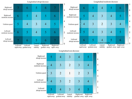
Figure 14.
Semantic Scoring Setting for Front Vehicle Role Feature Combinations.
Combining the scoring setup in Figure 14 and the labeling results in Figure 13, the driving style tendency score of driver Y as the front vehicle is calculated to be 4.72 using Equation (7):
where (i) represents the score of the i-th driving primitive segment, and N is the number of driving primitive segments.
- (2)
- Driving style tendency score as the rear vehicle
Similarly, when driver Y acts as the rear vehicle, K-means clustering is applied to its feature primitive segments, with the results distributed as shown in Figure 15.
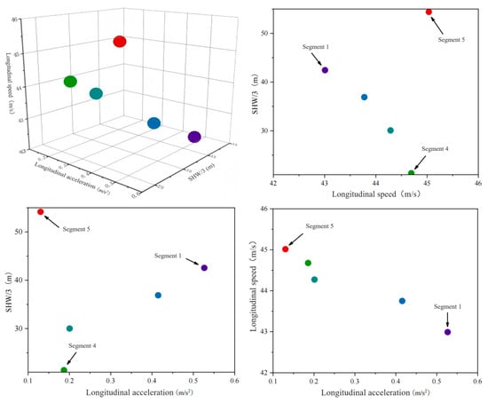
Figure 15.
Distribution of feature primitive segments after clustering as a rear vehicle.
Figure 16 shows the result of aggregation point marking of feature primitive fragments. It can be clearly seen that driver Y, as the rear vehicle, always keeps a long distance from the front vehicle, but has been driving at high speed in the longitudinal direction, accompanied by rapid acceleration and slow acceleration. These two situations indicate that the driver has overtaking or lane-changing intentions and has a clear pursuit of speed. In order to avoid potential risks, it is necessary to remind the target vehicle to pay attention to the distance from the rear vehicle at all times and maintain a safe distance so as to prevent the rear vehicle from approaching rapidly because of the pursuit of speed and avoid collision accidents.
Figure 16.
Characterization as a Rear Vehicle Based on Fragment Aggregate Point Labeling Results.
To evaluate the driving style tendency of driver Y as a rear vehicle, it is considered that maintaining a non-accelerating longitudinal speed and a relatively slow longitudinal velocity in long-distance situations is the safest driving behavior state. Therefore, the score for this condition is set to 1. As the risk level increases, the scores for the corresponding cells increase. Different from the scoring setup for the front vehicle, it is believed that constant longitudinal velocity, gradual deceleration, and sudden deceleration have little impact on the preceding lane-changing vehicle. Similarly, longitudinal slow speed and relatively slow speed also have minimal effects on the front vehicle, so the scores are set the same. When the headway distance gradually decreases, the increase in longitudinal velocity and acceleration poses a greater threat to the lane-changing vehicle, resulting in an increase in the corresponding cell scores.
Combining Figure 16 and Figure 17, the driver’s driving style tendency score as the rear vehicle is calculated as 5.98 points according to Equation (7). By studying the driving style preference of driver Y as the front and rear vehicles of the target vehicle, HDP-HSMM can reasonably segment the time series of driving trajectory, mine the semantic information expressed by each primitive segment, simply and efficiently evaluate the driving style preference, clearly show the driver’s driving behavior preference, and qualitatively describe and quantitatively score the driving style preference, so as to provide the quantitative analysis results of the driving style preference of other interactive vehicle drivers around the target vehicle, and provide the basis for the next step of risk prediction.
Figure 17.
Rear Vehicle Role Feature Combination Semantic Scoring Setting.
5. Conclusions and Prospects
5.1. Conclusions
In this study, the concept of “driving style tendency” was introduced into the short-term driving behavior analysis for the first time. Based on the driving behavior segmentation algorithm of HDP-HSMM, driving trajectory data were successfully divided into six front vehicle behavior segments and five rear vehicle behavior segments, with an average segmentation error of less than 0.1 s, and high time series processing accuracy. Through distribution fitting and threshold division, the classification accuracy of the model for longitudinal acceleration, lateral velocity, and other characteristic parameters is more than 90%, which verifies the effectiveness of feature extraction. Through the combination of a non-parametric Bayesian algorithm and K-means clustering, the automatic annotation of driving behavior semantic information is achieved. In a short-term driving segment randomly selected, when the driver is in the role of the car in front, the driving style tendency score is 4.72, indicating that the driver shows high lateral instability in the process of Lane changing, especially the behavior of rapid acceleration and deceleration, which poses a potential threat to the target vehicle; In the role of the rear vehicle, the score of driving style tendency was 5.98, which reflected that the driver showed high aggressiveness in longitudinal speed, especially in the behavior of close following and rapid acceleration, which increased the risk of collision. The results reveal the dynamic changes in driving style in lane-changing scenes, significantly improve the objectivity and explicability of driving style evaluation, and provide an important reference for the design of a personalized driving assistance system.
5.2. Future Prospects
Future research can be carried out in the following directions:
Future research directions include data expansion and generalization verification: introduce more diversified driving scene data (such as urban roads and bad weather) to improve the adaptability of the model to different traffic environments. Such extensions would enhance the robustness of the framework across dynamic real-world conditions, ensuring broader applicability beyond the constraints of existing datasets.
Real-time optimization: explore the application potential of the model in a real-time driving warning system by combining edge calculation or lightweight algorithm.
Man–machine cooperation mechanism: based on the driving style score, a dynamic interaction strategy is designed to optimize the cooperation efficiency between the automatic driving system and human drivers.
Further research is needed to investigate the different performances of parameters such as parking sight distance and headway distribution of vehicles under this model in road sections and intersections.
Author Contributions
Conceptualization, Y.J. and D.Q.; methodology, Y.J.; software, Z.Z.; validation, X.L.; investigation, X.L.; data curation, X.L.; writing—original draft preparation, Y.J. and Z.Z.; writing—review and editing, X.C. and D.Q.; project administration, Y.J.; funding acquisition, X.C. and D.Q. All authors have read and agreed to the published version of the manuscript.
Funding
This research was funded by the National Natural Science Foundation of China, grant number 52272311, Shandong Province Higher Education Youth Innovation Team Plan, grant number 2023KJ119, and Natural Science Foundation of Shandong Province, grant number ZR2023MG058.
Institutional Review Board Statement
Not applicable.
Informed Consent Statement
Not applicable.
Data Availability Statement
The original contributions presented in this study are included in the article. Further inquiries can be directed to the corresponding author.
Acknowledgments
The authors would like to express their gratitude to the project Modeling of driving safety potential field and resolving longitudinal and lateral dimensions steady-state response mechanism of vehicle clusters based on molecular dynamics in a connected environment for its support in providing essential resources and guidance for this study. This work benefited greatly from the collaborative research environment fostered by this program, which aims to promote the progress of driving safety and traffic technology.
Conflicts of Interest
The authors declare no conflicts of interest.
References
- Guo, Y.; Chen, Y.; Gu, X.; Guo, J.; Zheng, S.; Zhou, Y. Dynamic traffic graph based risk assessment of multivehicle lane change interaction scenarios. Phys. A Stat. Mech. Its Appl. 2024, 643, 129791. [Google Scholar] [CrossRef]
- Li, Y.; Yang, F.; Xuan, Z.; Zhou, B. Energy field-based lane changing behavior interaction model and risk evaluation in the weaving section of expressway. Traffic Inj. Prev. 2024, 25, 649–657. [Google Scholar] [CrossRef] [PubMed]
- Zhang, Y.; Chen, Y.; Gu, X.; Sze, N.; Huang, J. A proactive crash risk prediction framework for lane-changing behavior incorporating individual driving styles. Accid. Anal. Prev. 2023, 188, 107072. [Google Scholar] [CrossRef] [PubMed]
- Liu, T.; Wang, C.; Fu, R.; Ma, Y.; Liu, Z.; Liu, T. Lane-Change Risk When the Subject Vehicle Is Faster Than the Following Vehicle: A Case Study on the Lane-Changing Warning Model Considering Different Driving Styles. Sustainability 2022, 14, 9938. [Google Scholar] [CrossRef]
- Lee, S.E.; Olsen, E.C.B.; Wierwille, W.W. A Comprehensive Examination of Naturalistic Lane-Changes; National Highway Traffic Safety Administration: Washington, DC, USA, 2004. [Google Scholar]
- Eboli, L.; Mazzulla, G.; Pungillo, G. The influence of physical and emotional factors on driving style of car drivers: A survey design. Travel Behav. Soc. 2017, 7, 43–51. [Google Scholar] [CrossRef]
- Nori, R.; Zucchelli, M.M.; Cordellieri, P.; Quaglieri, A.; Palmiero, M.; Guariglia, P.; Giancola, M.; Giannini, A.M.; Piccardi, L. The prevention of road accidents in non-expert drivers: Exploring the influence of Theory of Mind and driving style. Saf. Sci. 2024, 175, 106516. [Google Scholar] [CrossRef]
- Padilla, J.L.; Sanchez, N.; Doncel, P.; Navarro-González, M.C.; Taubman–Ben-Ari, O.; Castro, C. The young male driving problem: Relationship between safe driving climate among friends, peer pressure and driving styles. Transp. Res. Part F Traffic Psychol. Behav. 2023, 98, 141–156. [Google Scholar] [CrossRef]
- Herrero-Fernández, D. Do people drive as they live, or are they transformed when they drive? A comparison of driving styles and living styles. Accid. Anal. Prev. 2021, 161, 106342. [Google Scholar] [CrossRef]
- Long, S.; Chang, R. Reliability and validity of the multidimensional driving style inventory in Chinese drivers. Traffic Inj. Prev. 2019, 20, 152–157. [Google Scholar] [CrossRef]
- Mensing, F.; Bideaux, E.; Trigui, R.; Ribet, J.; Jeanneret, B. Eco-driving: An economic or ecologic driving style? Transp. Res. Part C Emerg. Technol. 2014, 38, 110–121. [Google Scholar] [CrossRef]
- Reason, J.; Manstead, A.; Stradling, S.; Baxter, J.; Campbell, K. Errors and violations on the roads: A real distinction? Ergonomics 1990, 33, 1315–1332. [Google Scholar] [CrossRef] [PubMed]
- Ishibashi, M.; Okuwa, M.; Doi, S.; Akamatsu, M. Indices for characterizing driving style and their relevance to car following behavior. In Proceedings of the SICE Annual Conference 2007, Takamatsu, Japan, 17–20 September 2007. [Google Scholar]
- Taubman-Ben-Ari, O.; Mikulincer, M.; Gillath, O. The multidimensional driving style inventory—Scale construct and validation. Accid. Anal. Prev. 2004, 36, 323–332. [Google Scholar] [CrossRef] [PubMed]
- Sun, L.; Chang, R.S. Research status and Prospect of driving style. Ergonomics 2013, 19, 92–95. [Google Scholar]
- Huang, J.; Ji, Z.X.; Peng, X.Y.; Hu, L. Driving Style Adaptive Lane-changing Trajectory Planning and Control. China J. Highw. Transp. 2019, 32, 226–239+247. [Google Scholar]
- Totkova, Z. Subjective assessment of traffic rules compliance in Bulgaria: Role of personality and driving style. Transp. Res. Part F Traffic Psychol. Behav. 2024, 106, 370–384. [Google Scholar] [CrossRef]
- Eboli, L.; Mazzulla, G.; Pungillo, G. How to define the accident risk level of car drivers by combining objective and subjective measures of driving style. Transp. Res. Part F Traffic Psychol. Behav. 2017, 49, 29–38. [Google Scholar] [CrossRef]
- Hajiseyedjavadi, F.; Boer, E.R.; Romano, R.; Paschalidis, E.; Wei, C.; Solernou, A.; Forster, D.; Merat, N. Effect of environmental factors and individual differences on subjective evaluation of human-like and conventional automated vehicle controllers. Transp. Res. Part F Traffic Psychol. Behav. 2022, 90, 1–14. [Google Scholar] [CrossRef]
- Li, L.Z.; Yang, J.J.; Liu, S.X.; Guo, W.; Gao, J.; Ma, J.; Zhang, X.; Li, P.; Bai, B.; Nie, G. Research on driving style classification and recognition methods of domestic people. J. Chongqing Univ. Technol. 2019, 33, 33–40. [Google Scholar]
- Wang, X.; Ma, F.; Liao, X.L.; Zhang, W.; Wang, F. Screening of driving style characteristic indicators based on multi category supervised learning. Traffic Inf. Saf. 2022, 40, 162–168. [Google Scholar]
- Constantinescu, Z.; Marinoiu, C.; Vladoiu, M. Driving style analysis using data mining tech-niques. Int. J. Comput. Commun. Control 2010, 5, 654–663. [Google Scholar] [CrossRef]
- Zang, Y.; Wen, L.; Cai, P.; Fu, D.; Mao, S.; Shi, B.; Li, Y.; Lu, G. How drivers perform under different scenarios: Ability-related driving style extraction for large-scale dataset. Accid. Anal. Prev. 2024, 196, 107445. [Google Scholar] [CrossRef] [PubMed]
- Zhang, Y.H. Lane Change Risk Assessment and Decision-Making Method Based on Driving Style Identification and Motion Prediction; Xi’an University of Technology: Xi’an, China, 2020. [Google Scholar]
- Wan, Y.; Huang, M.H.; Wang, S.C. Research on driving style recognition method based on improved DBSCAN algorithm. J. Hefei Univ. Technol. 2020, 43, 1313–1320. [Google Scholar]
- Sun, P.; Wang, X.; Zhu, M. Modeling car-following behavior on freeways considering driving style. J. Transp. Eng. Part A Syst. 2021, 147, 04021083. [Google Scholar] [CrossRef]
- Liang, K.; Zhao, Z.; Li, W.; Zhou, J.; Yan, D. Comprehensive identification of driving style based on vehicle’s driving cycle recognition. IEEE Trans. Veh. Technol. 2023, 72, 312–326. [Google Scholar] [CrossRef]
- Hu, X.; Chen, S.; Zhao, J.; Wang, R.; Liu, W. Risk identification and prediction model for continuous-lane-change vehicles considering driving style. Expert Syst. Appl. 2025, 259, 125292. [Google Scholar] [CrossRef]
- Tawfeek, M.H.; El-Basyouny, K. A context identification layer to the reasoning subsystem of context-aware driver assistance systems based on proximity to intersections. Transp. Res. Part C Emerg. Technol. 2020, 117, 102703. [Google Scholar] [CrossRef]
- Zhao, S.S. Research on Short-Term Driving Style Evaluation Method Based on Driving Inclination; Jilin University: Changchun, China, 2021. [Google Scholar]
- Wei, C.B.; Qu, D.Y.; Kang, A.P.; Li, A.D.; Ji, L.Y. Modeling of lane changing behavior of networked autonomous vehicles based on risk potential field. Sci. Technol. Eng. 2024, 24, 8754–8760. [Google Scholar]
- Huang, J.; Chen, Y.; Peng, X.; Hu, L.; Cao, D. Study on the driving style adaptive vehicle longitudinal control strategy. IEEE/CAA J. Autom. Sin. 2020, 7, 1107–1115. [Google Scholar] [CrossRef]
- Yusof, N.M.; Karjanto, J.; Terken, J.; Delbressine, F.; Hassan, M.Z.; Rauterberg, M. The exploration of autonomous vehicle driving styles: Preferred longitudinal, lateral, and vertical accelerations. In Proceedings of the 8th International Conference on Automotive User Interfaces and Interactive Vehicular Applications, Ann Arbor, MI, USA, 24–26 October 2016; pp. 245–252. [Google Scholar]
- Lv, N.C.; Gao, J.J.; Wang, W.F.; Wang, Y.G. Driving style classification based on the characteristics of reduced headway in the net-worked environment. Traffic Inf. Saf. 2022, 40, 116–125+168. [Google Scholar]
- Richard, C.M.; Campbell, J.L.; Lichty, M.G.; Brown, J.L.; Chrysler, S.; Lee, J.D.; Boyle, L.; Reagle, G. Motivations for Speeding, Volume I: Summary Report; Department of Transportation, National Highway Traffic Safety Administration: Washington, DC, USA, 2012. [Google Scholar]
- Warriach, E.U.; Aiello, M.; Tei, K. A machine learning approach for identifying and classifying faults in wireless sensor network. In Proceedings of the 2012 IEEE 15th International Conference on Computational Science and Engineering (CSE), Paphos, Cyprus, 5–7 December 2012; pp. 618–625. [Google Scholar]
- Krajewski, R.; Bock, J.; Kloeker, L.; Eckstein, L. The highD dataset: A drone dataset of naturalistic vehicle trajectories on German highways for validation of highly automated driving systems. In Proceedings of the 2018 21st International Conference on Intelligent Transportation Systems (ITSC), Maui, HI, USA, 4–7 November 2018; pp. 2118–2125. [Google Scholar]


Disclaimer/Publisher’s Note: The statements, opinions and data contained in all publications are solely those of the individual author(s) and contributor(s) and not of MDPI and/or the editor(s). MDPI and/or the editor(s) disclaim responsibility for any injury to people or property resulting from any ideas, methods, instructions or products referred to in the content. |
© 2025 by the authors. Licensee MDPI, Basel, Switzerland. This article is an open access article distributed under the terms and conditions of the Creative Commons Attribution (CC BY) license (https://creativecommons.org/licenses/by/4.0/).