Abstract
Reliable and precise joint probabilistic forecasting of wind and solar power is crucial for optimizing renewable energy utilization and maintaining the safety and stability of modern power systems. This paper presents an innovative joint probabilistic forecasting model designed to address probabilistic spatiotemporal power output forecasting challenges. Leveraging a multi-network deep learning framework, the model integrated the temporal convolutional network for temporal feature extraction, the convolutional neural network for spatial feature analysis, and the attention mechanism for spatiotemporal focus enhancement, thereby capturing the spatiotemporal complementarity of wind and solar power. It also incorporated a quantile regression-based uncertainty quantification technique, contributing to reliable probabilistic predictions. A wind farm and two solar farms in China were used as a case study. Comparison results between the proposed model and ten established models demonstrated its superior performance in both reliable deterministic and probabilistic predictions, offering valuable insights for sustainable and resilient energy system operation.
1. Introduction
As fossil energy sources continue to deplete and the energy gap widens, nations worldwide are establishing carbon neutrality goals tailored to their conditions, hastening the development of diversified power systems with a focus on new energy sources [1]. Wind and solar energy, owing to their clean, renewable, and increasingly cost-effective qualities, are set to become the cornerstone of new power systems amid the transition to green and low-carbon energy structures [2,3]. In 2022, the installed capacity of renewable energy, primarily driven by wind and solar power, saw its largest increase to date [4]. The global installed capacity for renewable power generation grew by 9.6%, accounting for 83% of new power capacity, with wind and solar power capacity additions amounting to 78 GW and 240 GW, respectively [5]. However, as the proportion of wind and solar-based renewable energy in power systems increases, the inherent variability, unpredictability, and intermittency of these energy sources increasingly impact power system stability [6]. Wind and solar energy power systems are distinctly characterized by multiple uncertainties and limited interoperability among each other, posing greater challenges to integrated multi-energy power systems [7]. Accurate joint forecasting of wind and solar power is crucial to optimize the complementary nature of these sources, reduce the impact of the uncertainties of renewable energy on power grids, and enable large-scale grid integration of renewable energy.
Current wind and solar power forecasting models are primarily classified into three categories: physical, statistical, and machine learning models [8,9]. Physical models consider factors such as wind speed, wind direction, solar irradiance, and generator set characteristics [10]. They utilize meteorological principles and generator operation dynamics to create mathematical models for prediction. These models are noted for their high interpretability and stability in long-term forecasting. However, they demand significant computational resources, have complex modeling processes, and are less suited for short-term forecasting. Statistical models are derived from the analytical processing of historical data [11,12]. They are effective in stable conditions but less reliable in abnormal or unstable situations. These models often face challenges in handling non-linear relationships among variables, such as wind speed, solar irradiance, and power output [13]. Machine learning models, distinct from the other types, effectively extract complex non-linear relationships from diverse feature sets through extensive training on historical data [14,15,16,17]. They are increasingly utilized in wind and solar power forecasting, noted for their fast computational speed and versatility. Nevertheless, with increased feature dimensionality and extended forecasting horizons, traditional machine learning models often face difficulties in extracting more nuanced information [18].
Fortunately, the advent of deep learning models, particularly the Recurrent Neural Network (RNN) and the Convolutional Neural Network (CNN), has significantly mitigated many of these challenges [19,20]. Deep learning, a crucial branch of machine learning, utilizes a distributed and hierarchical feature representation approach. This approach allows for the effective extraction of more abstract and comprehensive information from high-dimensional data features. Through the application of diverse deep learning and artificial neural network algorithms, these advanced algorithms are integrated into the domain of renewable energy power forecasting [21]. A hybrid deep learning model, the bidirectional long short-term memory–convolutional neural network, was proposed by Zhen et al. for short-term wind power forecasting [22]. The convolutional neural network, the long short-term memory network, and the hybrid model based on the convolutional neural network and the long short-term memory network were all proposed by Wang et al. for day-ahead solar power forecasting [23]. An enhanced residual-based deep convolutional neural network was introduced by Yildiz et al. to forecast wind power [24].
Until recently, the topic of sequence modeling has predominantly centered around recurrent-like neural networks, which are favored for their superior performance in processing sequential data. In practice, RNNs must process data sequentially because of their inherent recurrent structure, posing challenges in capturing long-term dependencies due to phenomena like gradient vanishing or explosion in long sequences [25]. Alzubaidi et al. noted that traditional RNNs were becoming outdated and that advanced forms of CNNs should be considered as key alternatives for modeling sequential data [26]. The Temporal Convolutional Network (TCN), an emerging algorithm for time series prediction, was introduced by Bai et al. [27]. The TCN represents an advancement over traditional approaches. It synergizes the robust feature extraction capabilities of the CNN with the benefits of massively parallel computing. Simultaneously, it inherits the strengths of the RNN in effectively managing time series tasks, thereby encompassing the advantages of both methodologies [28]. Compared with the RNN, the TCN is generally more stable and exhibits stronger generalization capabilities, making it widely applicable in areas like wind and solar power forecasting [29,30].
A review of the above literature reveals that many scholars are actively engaged in wind and solar power forecasting research. However, existing forecasting approaches exhibit several key knowledge gaps.
- (1)
- The above deep learning models primarily concentrate on predicting power output of individual wind or solar farms. Given the expansive coverage of clean energy bases, single-site forecasts fall short in addressing the broader production needs.
- (2)
- Regarding issue (1), Yuan et al. examined independent, ensemble, and joint forecasting methodologies, and the findings indicate that ensemble forecasting of wind and solar power outputs yields higher accuracy compared with independent forecasting [31]. Zhang et al. introduced a joint forecasting approach for regional wind and solar power, and the results of the analysis indicate that the method not only enhances the accuracy of power predictions but also simultaneously provides predictions for each targeted station [32]. However, the above studies have tended to oversimplify the processing of heterogeneous energy input data from various energy sources, not adequately considering the distinct characteristics of each data type in their models.
- (3)
- Wind and solar farms are increasingly trending towards clustering, exhibiting a notable spatial correlation in their outputs within the region. Current research has not sufficiently accounted for these correlation patterns among farms in the joint forecasting modeling, thereby hindering advancements in prediction accuracy.
- (4)
- Deterministic forecasting models often fail to account for the uncertainty associated with power output and its quantification when forecasting the generation of wind and solar plants. This limitation can result in inaccurate and unreliable forecasts, potentially compromising the stability and operational planning of the power system.
Therefore, to address the aforementioned issues, a novel joint probabilistic forecasting model of wind and solar power outputs, called the Spatiotemporal Multi-network Joint Probabilistic (SMJP) model, was proposed in this paper. This model employed a multi-network deep learning framework, achieving precise deterministic predictions for wind and solar power by combining the TCN’s temporal feature extraction, the CNN’s spatial feature mining, and the AM’s spatiotemporal focus enhancement. It also incorporated a quantile regression-based uncertainty quantification technique, providing reliable probabilistic predictions. To validate the superiority of the proposed SMJP model, a wind farm and two solar farms located in the western Ningxia Hui Autonomous Region of China were applied to assess the forecasting performance. The proposed model effectively facilitates the development of a spatiotemporal forecasting framework for joint wind and solar power across the entire region, contributing to the broader goals of clean energy transition and sustainable power system development.
2. Methodologies
In this section, the TCN and the forecasting models are introduced initially, and then the quantile regression method is described. Finally, the evaluation indices used in this paper are given.
2.1. Temporal Convolutional Network (TCN)
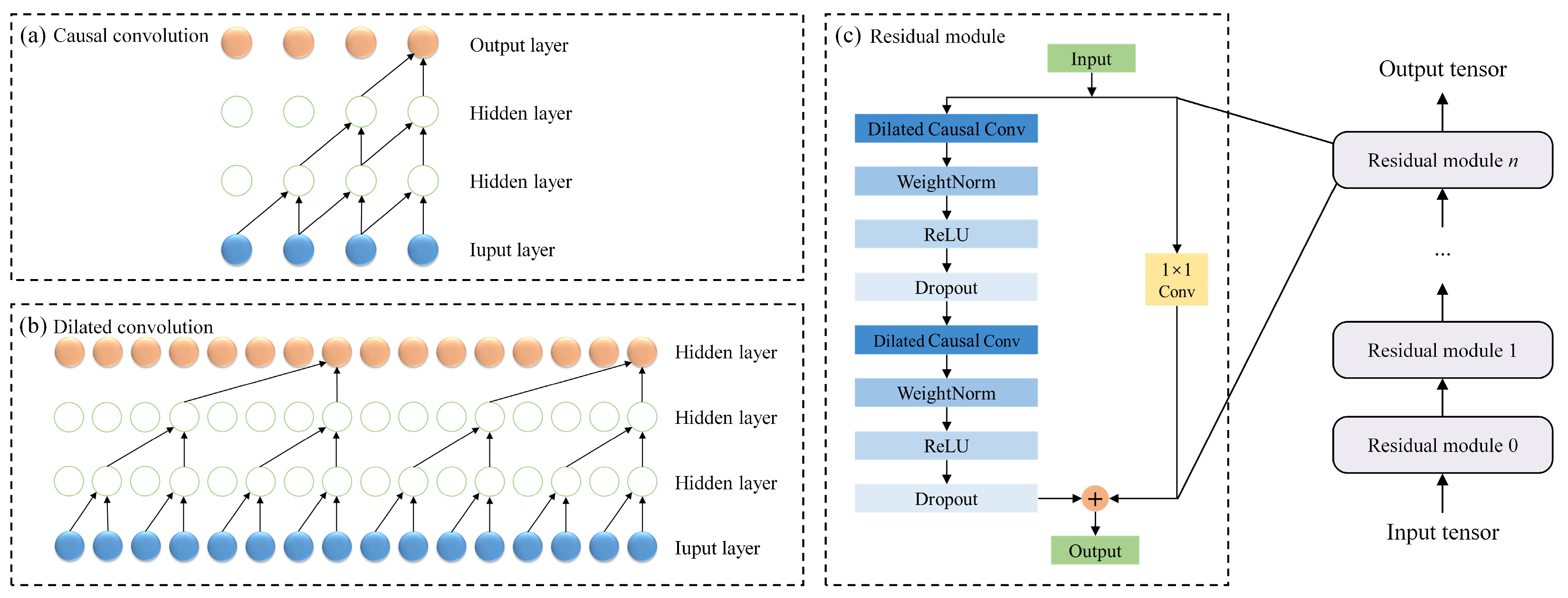
The main structure of the TCN comprises causal convolution, dilated convolution, and a residual module. These elements are illustrated in Figure 1. The distinguishing characteristics of the TCN include: (a) the ability to take a sequence of any length and map it to an output sequence of the same length, akin to the RNN; (b) the incorporation of causal convolutions within its architecture, ensuring no information leakage from future to past. To accomplish the first characteristic, the TCN adopts a 1D fully convolutional network architecture. Each hidden layer can be maintained at the same length as the input layer, achieved by adding zero padding of the appropriate length. This padding ensures that the lengths of subsequent layers remain consistent with previous ones. For the second characteristic, the TCN employs causal convolutions, where an output at time t is convolved only with elements from time t and earlier in the previous layer, preventing any future data influence. As a variant of the CNN, the TCN employs a convolutional structure that effectively captures local temporal dependencies. Moreover, expanding the receptive field enables the capture of richer input features, supports parallelized feature extraction and prediction, and thus enhances overall forecasting performance [33].
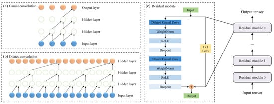
Figure 1.
Schematic diagram of TCN components.
- (1)
- Causal convolution
Causal convolution is a special type of convolution, which is achieved by appropriately filling the input data. The concept of causal convolution is well illustrated in Figure 1a. Essentially, the value at time t in a given layer depends solely on the value at time t and its predecessors in the preceding layers. The key distinction between causal convolution and the traditional CNN is that causal convolution cannot access future data. This results in a unidirectional, as opposed to a bidirectional, flow of information.
- (2)
- Dilated convolution
While causal convolution presents improvements in certain aspects, it encounters a significant limitation common to the traditional CNN: the capacity for temporal modeling is constrained by the filter size. To overcome this, the TCN utilizes dilated convolution. For a filter , sequence , the mathematical representation of the dilated convolution operation is given by [34]
where K is the filter size, represented by the maximum value of k, and d is the dilation rate, determining the spacing between the inputs in the convolution.
Utilizing dilated convolution enables convolutional networks to acquire a larger receptive field using fewer layers. The structure of the dilated convolution is illustrated in Figure 1b. In this manner, the CNN can achieve a large receptive field with relatively few layers. Dilated convolution represents a significant advancement in CNN architecture [35].
- (3)
- Residual module
In a network with increasing layers, gradient disappearance (or vanishing) becomes a notable challenge. Residual connections help mitigate this issue by allowing gradients to flow through the network more effectively. The formula for a residual module is typically given as
where is the residual output, represents the activation function, denotes the residual channel, and indicates the convolutional operation module.
A residual module comprises two layers of convolution and a residual connection, with WeightNorm and Dropout incorporated into each layer to regularize the network. The structure of the residual module is depicted in Figure 1c. The input data is initially processed through a dilated convolutional layer, which enables the capture of information at varying time scales. Thereafter, the convolved output is integrated with the original input to generate the output of the residual block. The design of this residual connection serves to reduce the loss of information during network transmission, thereby enabling it to perform more effectively in processing time series data.
2.2. Construction of Forecasting Models
This paper detailed the development of three distinct types of models: the independent forecasting model, the joint forecasting model, and the spatiotemporal multi-network joint forecasting model, as outlined below. From independent models to joint models and, finally, to spatiotemporal multi-network joint models, this progressive model refinement strategy enables a comparative and interpretable evaluation of the benefits of spatiotemporal integration.
- (1)
- Independent Forecasting Model
Utilizing the TCN framework, Independent Temporal Convolutional Network (ITCN) forecasting models for each farm have been developed. Specifically, the independent model at the wind farm took in the previous historical wind power and meteorological data to predict the ensuing wind power output [36]. Similarly, the independent models at the two solar farms used the previous historical solar power and meteorological data to predict the ensuing solar power output [30].
- (2)
- Joint Forecasting Model
Utilizing the TCN framework, a Joint Temporal Convolutional Network (JTCN) forecasting model for all of the farms had been developed. Unlike the independent models, this joint model processed the previous historical power and meteorological data from all farms to predict the ensuing wind and solar power outputs.
- (3)
- Spatiotemporal Multi-network Joint Forecasting Model
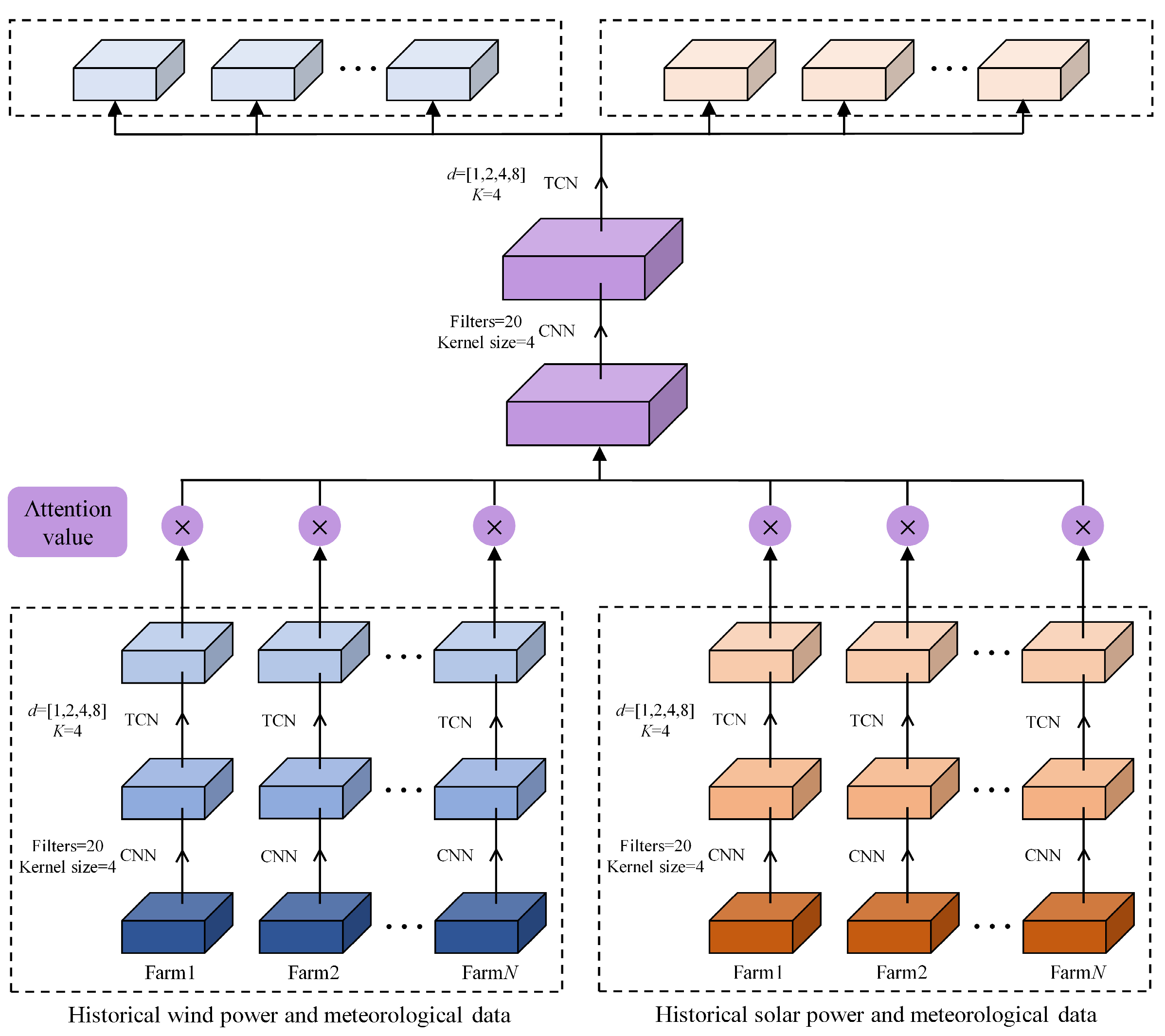
Most joint forecasting models often oversimplify the treatment of heterogeneous energy inputs, leading to inadequate consideration of the differences among various data types. The previously discussed joint forecasting model did not differentiate between variable types, neglecting the unique attributes of each data type. Therefore, a Spatiotemporal Multi-network Joint (SMJ) forecasting model was proposed and trained. The SMJ model, accommodating the different data dimensions of the input and output modules, adopted a sequence-to-sequence architecture to better map the relationship between input and output sequences. It utilized the TCN for temporal feature extraction and the CNN for spatial feature extraction, integrated with an Attention Mechanism (AM) for highlighting critical features in spatiotemporal sequences. The model independently processed various energy sources before their integration, thereby improving the extraction of spatiotemporal features from regional wind and solar resources. The complete modeling process is detailed in Figure 2. First, the input variables of the wind and solar farms were encoded separately to preliminarily represent the temporal features of the historical input variables. Subsequently, the forecasting framework incorporated the CNN and the TCN to extract hidden spatiotemporal features and capture potential correlations between the data. Furthermore, the AM was introduced to strengthen the feature extraction capability of the model. Finally, the CNN and the TCN were employed to decode the fused feature matrix, thereby obtaining the output data. Figure 2 involves multiple components, but the forecasting process is not complicated, as each major component is logically integrated. While considering complex spatiotemporal relationships, there is no significant increase in computation time.

Figure 2.
Schematic diagram of forecasting framework.
The SMJ forecasting model makes the following contributions. (i) The SMJ model is a key novelty of our work. It enhances conventional TCN-based forecasting by: ① Separating the input encoding by energy type to retain data heterogeneity; ② integrating the CNN for spatial feature extraction and the AM to dynamically highlight important spatiotemporal features; and ③ using a sequence-to-sequence structure that effectively maps multivariate historical data to future power outputs. (ii) Unlike prior TCN applications that focus solely on temporal patterns, our SMJ model explicitly couples spatial and temporal dimensions. This is particularly important when modeling interactions between spatially distributed renewable energy sources (wind and solar) over a wide geographic area.
2.3. Quantile Regression Method
Quantile regression offers a more nuanced view compared with traditional regression methods, as it reveals the entire conditional distribution of predicted outcomes, rather than focusing solely on the central tendency. Notably, quantile regression focuses on determining the relationship between a specific quantile (such as the median or another percentile) of the dependent variable and the independent variables. It calculates a particular quantile by minimizing the total absolute deviations between the observed and predicted values. The quantile regression model can be expressed by
where is the probability that the dependent variable is less than or equal to value , denotes the minimum value of when is greater than or equal to , represents the conditional quantile of the dependent variable under the independent variables , and indicates a vector of parameters for quantile . The parameters were estimated by minimizing the loss function for a particular quantile.
Before optimizing the quantile regression, the loss function was defined, and the optimal parameters were estimated by minimizing the loss function, which is given by
From Equation (5), it becomes clear that, after estimating the parameter vector , one can assess the impact of the independent variables on the conditional quantile of the dependent variable for various values. By varying continuously over the interval (0, 1), one can derive the conditional distribution of the dependent variable. Subsequently, this facilitates the estimation of the conditional density function and enables predictive density estimation.
2.4. Indices for Model Evaluation
In this study, the Mean Absolute Error (MAE), Root Mean Square Error (RMSE), and Coefficient of Determination (R2) were used to evaluate the deterministic prediction accuracy of the models. The MAE and RMSE quantify the difference between predicted values and actual observations, serving as measures of predictive accuracy. The R2, a statistic reflecting the model’s goodness of fit, indicates how well the model explains the variability of the data. A smaller MAE and RMSE imply higher prediction accuracy. Conversely, a larger R2 indicates a better fit. The specific formulas are given as follows.
where is the total number of observations, represents the predicted values, represents the measured values, denotes the average of the predicted values, and denotes the average of the measured values.
Common evaluation indices for probabilistic prediction include reliability, sharpness, and a Skill Score [37]. Reliability assesses the prediction model probabilistically by comparing the actual probability of the real value falling within the prediction interval against the pre-set probability. A model can be deemed reliable if the actual probability is greater than or equal to the predetermined probability. Otherwise, it is considered less reliable. Sharpness assesses the model based on the prediction interval’s width. A smaller sharpness, indicating a narrower prediction interval, indicates better model performance, assuming reliability is maintained. Neither reliability nor sharpness alone offers a comprehensive evaluation of probabilistic forecasting models. High sharpness may naturally satisfy reliability. However, without reliability, sharpness is meaningless. Hence, this study utilizes the Skill Score, which evaluates both reliability and sharpness for an all-encompassing assessment of the prediction model’s uncertainty. A higher Skill Score indicates a stronger overall performance of the model. The formula for calculating the Skill Score at the quantile is given as
where represents the predicted values at the quantile, denotes a binary variable characterizing whether the measured value is greater than the predicted value at the quantile, indicates the Skill Score at the quantile, and is the Skill Score calculated at the 1 − β confidence level.
3. Case Study
In this section, the descriptions of the experimental dataset and the correlation analysis of wind and solar power outputs are introduced first, followed by the detailed setup of the comparative experiment and the methodology for model training.
3.1. Study Area and Data Sources
To validate the proposed model, three sets of power and meteorological data gathered from a wind farm and two solar farms located in the western Ningxia Hui Autonomous Region of China were applied to assess the forecasting performance. The dataset comprises wind speed (WS: m/s) and wind power (WP: MW) from the Kaige 2nd Wind Farm (WF1), along with solar irradiance (SI: W/m2) and solar power (SP: MW) from the Zhongwei 54th and 74th Solar Farms (SF1 and SF2), collected at 15 min intervals from 1 January 2022 to 31 July 2023. WF1 is located at 105°25′9″ east longitude and 37°35′42″ north latitude. SF1 is located at 105°20′25″ east longitude and 37°30′52″ north latitude. SF2 is located at 105°18′33″ east longitude and 37°38′12″ north latitude. Figure 3 shows the locations of these three farms. While WF1, SF1, and SF2 are located in the same general region, they are not geographically co-located. By jointly modeling these sites, we enhance forecasting robustness and assess the model’s spatial generalization capability. In real-world scenarios, nearby wind and solar farms often form spatial clusters, and understanding their collective dynamics is crucial for effective regional grid integration. In this study, the input sequence length is set to 16 time steps (equivalent to 4 past hours) by utilizing a trial-and-error approach. Therefore, the forecasting models employed the previous 4 h historical power and meteorological data to predict the ensuing 2 h sequence of wind and solar power. In addition, the data were divided into a training set, a validation set, and a test set in an 8:1:1 ratio.
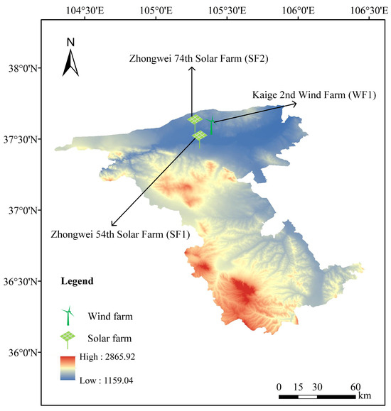
Figure 3.
Three farms and their locations in Zhongwei City, Ningxia Hui Autonomous Region.
In the same region, wind and solar farms are impacted by local geographical and climatic conditions, leading to notable spatiotemporal correlations in power output. The power forecasting modeling process necessitates an investigation into the spatial coupling of these diverse energy sources (wind and solar), as well as the temporal relationships between historical power/meteorological data and present power output. Gaining insights into these aspects is crucial for greatly enhancing the accuracy of power forecasting models.
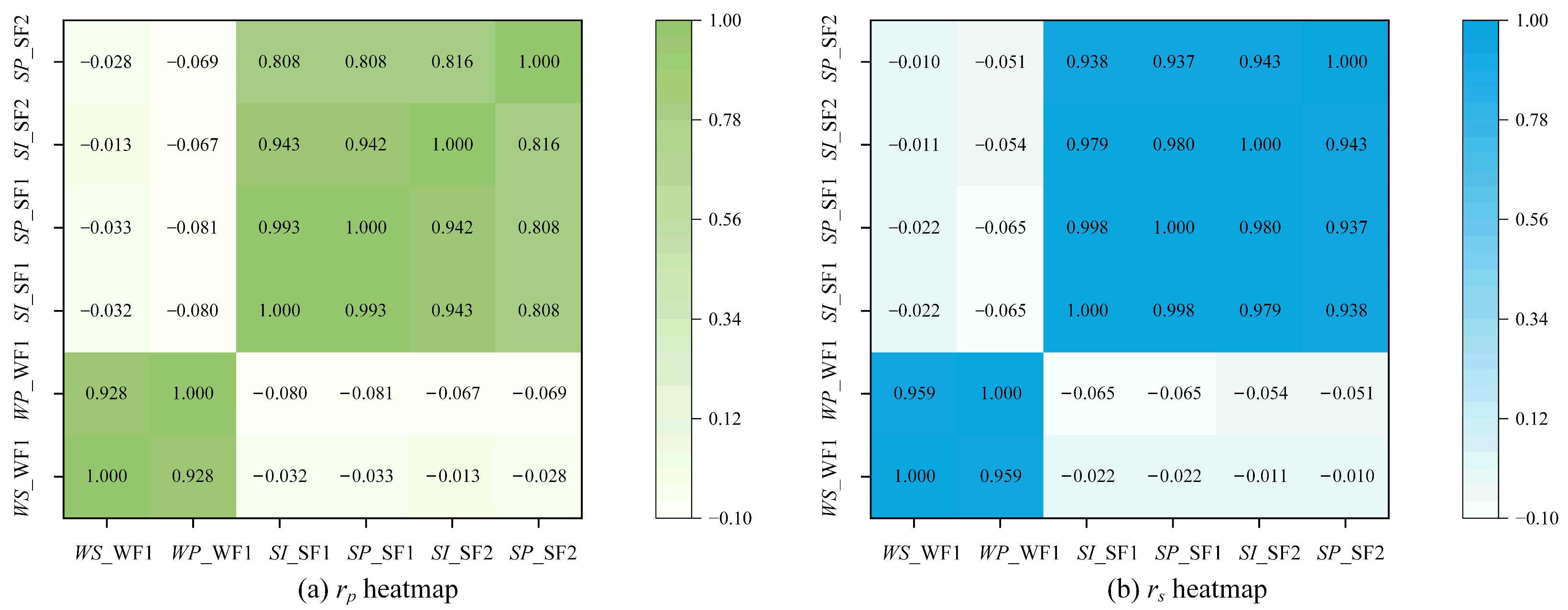
The Pearson correlation coefficient and the Spearman correlation coefficient were used to quantitatively analyze the correlation between various parameters of the wind and solar farms. Results are presented in Figure 4, which shows a strong correlation between power and meteorological data within the farms. In WF1, the and between wind power and wind speed are 0.928 and 0.959, respectively. In SF1, the and between solar power and solar irradiance are 0.993 and 0.998, respectively. In SF2, the and between solar power and solar irradiance are 0.816 and 0.943, respectively. High positive correlations were also observed between energy sites of the same type, indicating similar performance patterns. The and between the solar power of SF1 and SF2 are 0.808 and 0.937, respectively. The correlation between heterogeneous energy sources, specifically between wind and solar power, was quite low, ranging from −0.032 to −0.011, suggesting significant differences in the characteristics and variability of these energy types. The Pearson and the Spearman correlation analyses were used during the exploratory data analysis phase to assess the monotonic relationships between input variables and power output. Although the final forecasting model is non-linear, such analyses help identify informative variables and understand their general directional influence, which enhances model interpretability.

Figure 4.
Heat map of the correlation between different wind and solar parameters.
During the modeling process, different energy sources, such as solar and wind, were coded separately and then combined to extract the spatiotemporal characteristics of the region. The Pearson and the Spearman correlation coefficients also provide insight into potential redundancy or complementarity among input features (meteorological variables across different farms), helping to justify the structure of the input representation and multi-source fusion strategy. This approach improved the accuracy of the predictions by leveraging the complementary nature of solar and wind energy variability.
3.2. Experimental Design
To assess the efficacy of the SMJP forecasting model, both independent and joint probabilistic forecasting models were constructed for comparative analysis. Specifically, Section 2.2 outlines three probabilistic forecasting model development approaches. Probabilistic forecasting models adopted the quantile regression method for uncertainty quantification as described in Section 2.3. To integrate quantiles into the model architecture, the forecasting models were trained using the pinball loss function, enabling the direct prediction of multiple quantile levels. This approach allows the models to capture the uncertainty in future power outputs by generating prediction intervals rather than single-point estimates. The resulting quantile forecasts provide valuable insights into the distribution and variability of power generation, supporting more informed and risk-aware operational decisions. These models, including the SMJP, were implemented using the ‘Keras 2.3.1’ framework within the Python 3.8.0 programming environment. The computations are performed on a high-performance system equipped with an Intel Core i9-12900H CPU (2.5 GHz) (Santa Clara, CA, USA), 16 GB RAM, and Windows 10.
In tackling the challenges of spatiotemporal probabilistic forecasting, distinct sample sets had been allocated to various models. Each sample’s feature and label were structured as a 2-dimensional matrix, denoted as , , where symbolizes the input sequence length, encapsulates the historical power and meteorological variables, indicates the output sequence length, and signifies the power prediction features. To optimize the performance and mitigate overfitting, all deep learning models in this study implemented settings that include a mini-batch size of 128, a maximum iterations number of 200, min–max normalization, an early stopping strategy, and a learning rate decay mechanism.
4. Comparison Results and Discussion
In this section, the performance of proposed model are validated in terms of deterministic prediction, probabilistic prediction, and the reliability of probabilistic forecasting. For deterministic prediction models, the MAE, RMSE, and R2 are used as key indices to evaluate improvements in forecasting performance. For probabilistic models, forecasting improvements are assessed by comparing the Skill Scores.
4.1. Evaluation of Deterministic Prediction
To verify the prediction accuracy of the SMJ model, deterministic prediction indices for the Persistence (PR), Ridge Regression (RR), XGBoost, Transformer, ITCN, JTCN, Independent Long Short-Term Memory (ILSTM), Joint Long Short-Term Memory (ILSTM), Independent Gated Recurrent Unit (IGRU), Joint Gated Recurrent Unit (JGRU), and SMJ models are presented in Table 1. The average prediction error for the 2 h ahead power output in wind and solar farms was calculated. As indicated in the table, the proposed SMJ model achieved the highest comprehensive score among all models, while the PR model recorded the lowest comprehensive score. In WF1, the ITCN model surpassed the ILSTM model, showing a 0.31% decrease in the MAE, a 1.16% decrease in the RMSE, and a 3.08% increase in the R2. In comparison with the IGRU model, it displayed a 0.81% lower MAE, a 1.61% lower RMSE, and a 3.59% higher R2, highlighting that the TCN has strong predictive capabilities in the realm of independent forecasting models. In SF1, the ITCN model outperformed the ILSTM model, demonstrating a 1.11% decrease in the MAE, a 1.90% decrease in the RMSE, and a 0.66% increase in the R2. When compared with the IGRU model, it exhibited a 3.12% lower MAE, a 1.32% lower RMSE, and a 0.55% higher R2. This pattern was also observed in SF2. These results demonstrate that the TCN model notably improved the R2 more than it impacted the MAE and RMSE in WF1, and, conversely, it more effectively lowered the MAE and RMSE than it affected the R2 in SF1 and SF2.

Table 1.
Deterministic prediction indices for seven models in three farms.
In a comparative analysis between independent and joint forecasting models, the joint forecasting models each consistently outperformed their independent counterparts, respectively. In WF1, the JTCN model outperformed the ITCN model, exhibiting a 0.46% lower MAE, a 1.10% lower RMSE, and a 0.51% higher R2. The pattern of performance was consistently observed in both SF1 and SF2. This demonstrates that utilizing a joint prediction approach can lead to enhanced prediction accuracy. In addition, mirroring the pattern where the ITCN surpassed the ILSTM and IGRU, the JTCN also consistently outperformed the JLSTM and JGRU in all the farms. This further validates the robust predictive capabilities of the TCN model in both independent and joint forecasting contexts. Moreover, the proposed SMJ model is identified as the optimal choice among all deterministic forecasting models. The effectiveness is attributed to the model’s integration of the TCN’s temporal feature mining, the CNN’s spatial feature mining, and the AM’s spatiotemporal focus enhancement capabilities. This approach facilitates the extraction of spatiotemporal correlation features of the farms, leading to improved prediction accuracy. Additionally, the SMJ model demonstrates greater stability in its predictions compared with conventional joint forecasting models. In WF1, the SMJ model consistently outperformed the JTCN model, with a 0.33% reduction in the MAE, a 0.60% reduction in the RMSE, and a 0.38% improvement in the R2. In SF1, the SMJ model further extended its lead over the JTCN model, showing a 3.34% reduction in the MAE, a 1.15% reduction in the RMSE, and a 0.22% improvement in the R2. In SF2, the SMJ model maintained its superior performance against the JTCN model, indicating a 0.22% reduction in the MAE, a 1.90% reduction in the RMSE, and a 0.66% improvement in the R2. Notably, although the predictions across the ten models were relatively close, a clear ranking emerged, with the SMJ model outperforming the others. Compared with the independent models, the runtime of the joint models increased due to the larger number of input features. The proposed SMJ model had the longest runtime, but it achieved the best predictive performance. Therefore, when the computation time limit is approximately 100 s or more, this model is preferred.
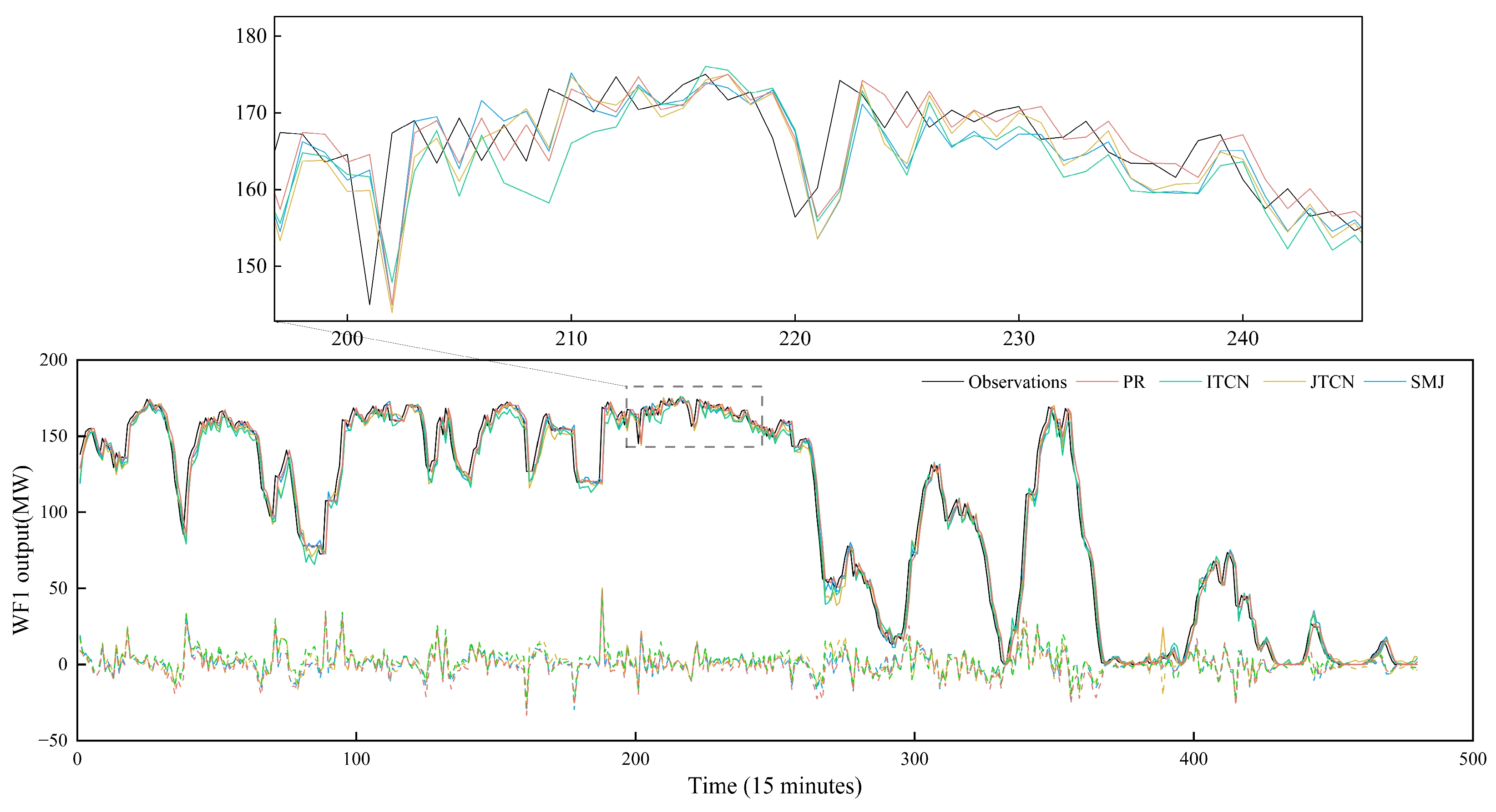
We randomly selected the 15 min ahead wind power output (excluding solar power output) for five representative days in order to evaluate the model’s predictive accuracy. Figure 5 showcases the visual comparative results calculated by the PR, ITCN, JTCN, and SMJ models. The figure illustrates the comparison between predicted and actual values, including their corresponding errors. The analysis demonstrated that the SMJ model displayed minimal error magnitudes, with all evaluation indices showing slight improvements. In summary, the SMJ model demonstrated superior capability in providing high-precision deterministic prediction results relative to the other models when comparing the independent forecasting and the joint forecasting of output.
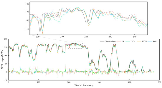
Figure 5.
Comparison of wind power output across the three forecasting models.
4.2. Evaluation of Probabilistic Prediction
This study utilized predicted power output as the independent variable and prediction error as the dependent variable in the quantile regression analysis. To test the applicability of the prediction intervals obtained from the SMJP model, analyses involving the ITCNP and JTCNP models were conducted. These models were ranked third and second, respectively, in the overall model rankings. The probabilistic prediction index—the Skill Score—was employed to assess the uncertainties and accuracy of the three probabilistic forecasting models in a comprehensive manner, and the results are presented in Table 2. As clearly shown in the table, probabilistic predictions for power output from the wind and solar farms at three commonly used confidence levels (90%, 80%, and 70%) were collated and analyzed. The average Skill Score for the 2 h ahead power output from the wind and solar farms was calculated. The data presented in Table 2 indicates that the SMJP model outperformed the ITCNP and JTCNP models in terms of probabilistic prediction across various confidence levels. The SMJP model secured the highest Skill Score among all the wind and solar farms, demonstrating its superior stability in probabilistic interval forecasting. It was followed by the JTCNP model in second place, with the ITCNP model ranking last. This observation indicates a relationship between the effectiveness of deterministic and probabilistic forecasting methods. Specifically, models that demonstrate high accuracy in deterministic forecasting are likely to produce superior interval forecasting outcomes. Conversely, models with lower accuracy in deterministic forecasting tend to exhibit less effective interval forecasting performance. Additionally, a notable trend of enhanced improvement is observed in the probabilistic prediction for both the wind and solar farms at increased confidence levels.
Table 2.
Model Skill Scores at 90%, 80%, and 70% confidence levels.
Analysis of the table reveals that the JTCNP model’s probabilistic prediction performance is superior to that of the ITCNP model. Consequently, the subsequent discussion will focus on the probabilistic Skill Scores of the SMJP and JTCNP models. In WF1, the probabilistic prediction Skill Scores at 90%, 80%, and 70% confidence levels showed increments of 0.13%, 0.34%, and 0.55%, respectively. In SF1, the increases in the Skill Score were 2.07%, 3.00%, and 3.51%. In SF2, the respective increases were 2.68%, 2.37%, and 1.85%. This method demonstrates a distinct edge in probabilistic prediction for solar power over wind power. Notably, in WF1 and SF1, lower confidence levels were linked to more substantial improvements in probabilistic prediction, while in SF2, the trend reversed, with higher confidence levels yielding more significant improvements. In summary, the proposed SMJP model will achieve higher forecasting accuracy and better probabilistic calibration than comparable models by capturing cross-source interactions, spatiotemporal dependencies, and uncertainty information. Additionally, the prediction intervals generated by the model are adaptive rather than fixed or symmetric, varying in response to the spatiotemporal characteristics of the input data. This enables the model to capture elevated uncertainty during rapid power fluctuations, while narrowing intervals under stable conditions. In practical applications, this behavior is critical for system operators, as it provides not only point forecasts but also confidence intervals that support reserve allocation and risk-informed decision-making processes. Quantile-based probabilistic forecasting effectively captures the heteroscedasticity inherent in renewable power output, which traditional deterministic models tend to neglect.
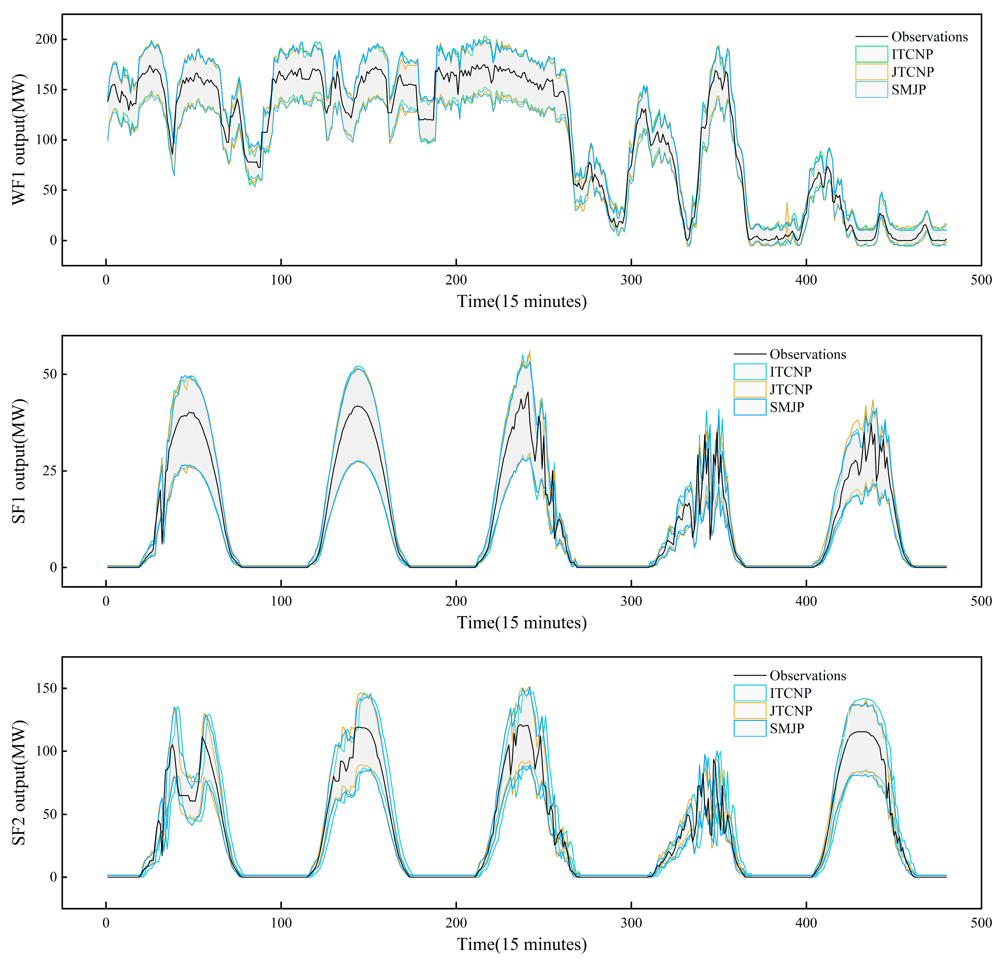
For a clearer visualization of the interval prediction results from each model, Figure 6 displays the 15 min ahead interval prediction outcomes for the three models across all farms. It features the same five days as mentioned earlier, set at a 90% confidence level. Of the three models, the SMJP model demonstrates the most balanced prediction interval, striking a midpoint between being overly conservative and excessively optimistic. In summary, the SMJP model demonstrates superior capability in providing high-precision interval prediction results relative to other models.
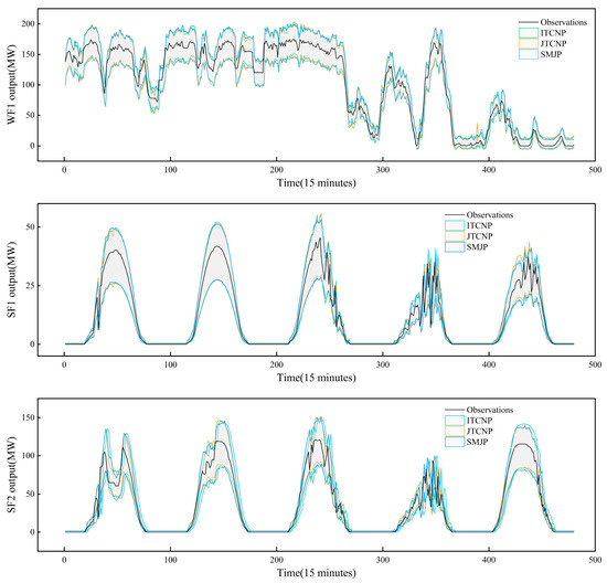
Figure 6.
The 15 min ahead 90% interval predictions for the three models.
4.3. Reliability Evaluation of Probabilistic Forecasting
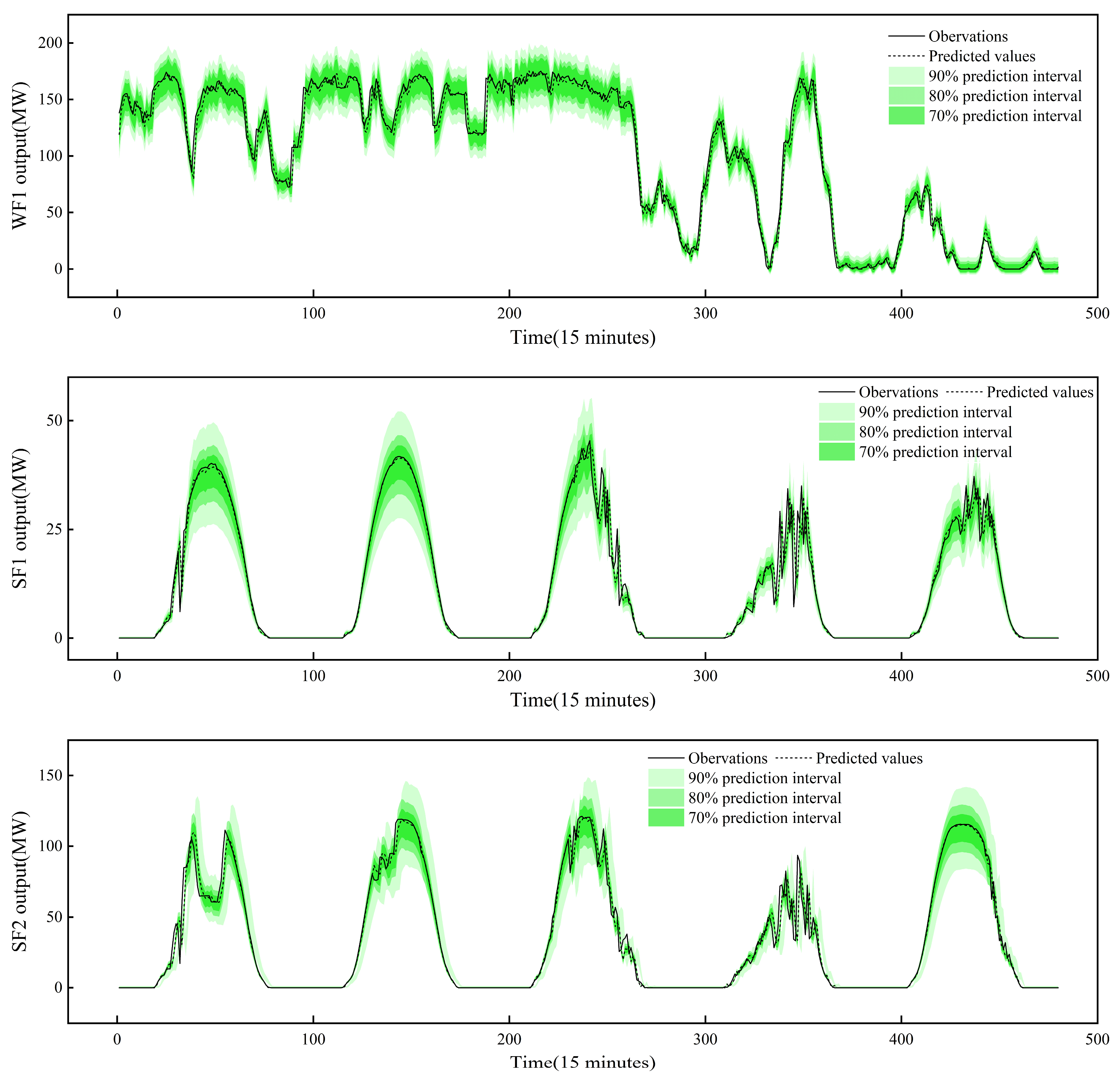
In the preceding subsections, the multi-model comparison approach was employed. In this subsection, the focus will shift to the reliability assessment of the proposed model’s probabilistic predictions using the self-assessment technique. Notably, the data selected from the previous subsections was used for a reliability analysis. Figure 7 illustrates the SMJP model’s predicted values and quantile ranges in three farms. The greater the proximity of the prediction to the observed values, the higher is the accuracy of the prediction. Additionally, the more observations that fall within the prediction interval, the greater the reliability of that interval. The graph demonstrates that the predictions closely resemble the observed values, with the majority being within 90% of the prediction intervals.

Figure 7.
Predicted values and quantile ranges of SMJP model.
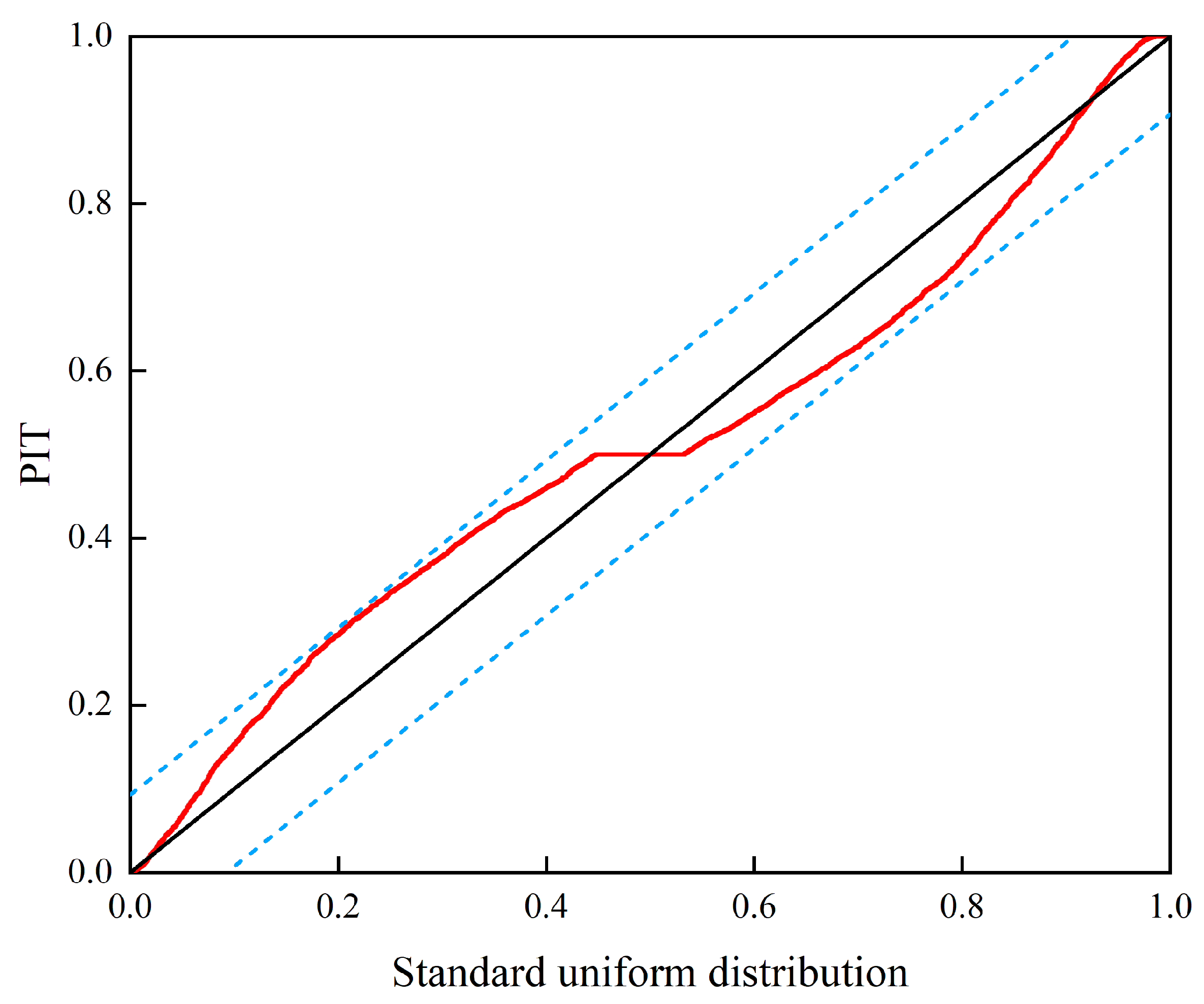
For convenience, WF1 is used as an example in the following two figures. Figure 8 presents the uncertainty estimation of the test set. Here, the proximity of points to the 1:1 line signifies the accuracy and reliability of the predictions. This figure shows that the relationship between the observed and predicted power output aligns closely with the 1:1 line, predominantly within the 90% prediction range. This suggests that the SMJP model effectively captures spatiotemporal power fluctuations and offers both dependable deterministic and interval predictions. Further bolstering our findings, Figure 9 displays the Probability Integral Transformation (PIT) diagram for the SMJP model. The black straight line represents a 1:1 line, while the red points depict the linear relationship between the PIT values and the standard normal distribution. Overestimated uncertainty is indicated by PIT points leaning towards the upper left of the black line, while underestimation is shown by a skew towards the lower right. As shown in Figure 9, all PIT points are evenly distributed along the diagonal, falling within the Kolmogorov 5% significance band (blue dashed line), signifying reasonable and credible probabilistic predictions. Overall, the SMJP model is demonstrated to provide trustworthy probabilistic predictions.
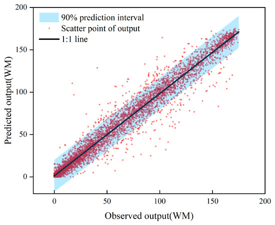
Figure 8.
Uncertainty estimation of SMJP model.
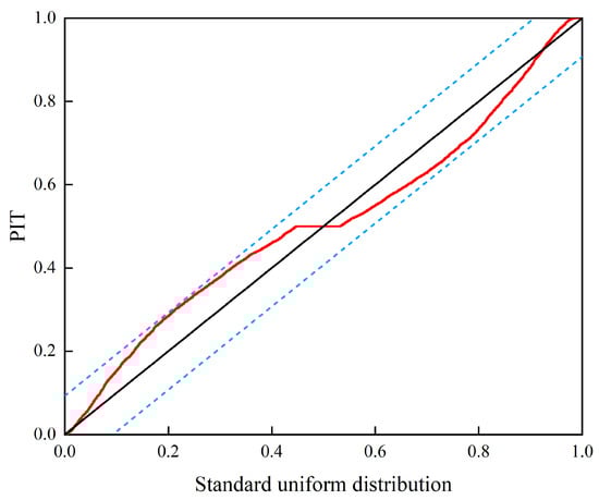
Figure 9.
PIT diagram of SMJP model.
5. Conclusions
This paper introduces a unique joint probabilistic forecasting model that forecasts wind and solar power outputs in a region using multi-site historical data. This model utilizes the TCN and quantile regression as its foundation. It employs a multi-network deep learning approach, achieving precise spatiotemporal predictions for wind and solar power by combining the TCN’s temporal feature extraction, the CNN’s spatial feature mining, and the AM’s spatiotemporal focus enhancement. Additionally, it includes an uncertainty quantification method based on quantile regression, ensuring dependable probabilistic forecasts. Applied in a case study within the Ningxia Hui Autonomous Region of China, the model’s effectiveness was evaluated using three farms, four evaluation indices, and ten benchmark models, assessing its performance in various dimensions. The experimental findings confirmed that the model excelled in delivering not only high-precision deterministic forecasts but also appropriate interval predictions and trustworthy probabilistic outcomes. By supporting more accurate forecasting and uncertainty estimation, the model contributes to the more efficient integration of renewable energy sources, aligning with the broader objectives of clean energy transition and sustainable power system development.
However, the variability in weather conditions contributes to the uncertainty and fluctuation in wind and solar power output sequences, thereby complicating the prediction process. In the future, to enhance the overall practical applicability and performance of the proposed model, the following measures can be considered.
- (1)
- Although the model was trained on a specific region, it has a modular and data-driven architecture, allowing it to be retrained or fine-tuned on datasets from other regions. Components such as the CNN (for spatial pattern learning) and the AM help adapt to varying spatial correlations, which is beneficial for generalization across locations. In future research, we plan to test the model on multi-regional datasets to further validate its robustness and extendibility. Transfer learning or meta-learning techniques will be explored to adapt the model to new locations with limited training data.
- (2)
- Given the proposed model’s exhibited scalability, future research aims to develop more sophisticated models to tackle spatiotemporal forecasting challenges. Meanwhile, the training dataset will be partitioned based on regional weather patterns to better accommodate diverse future weather conditions. These improvements are planned to be applied across broader and more intricately detailed regions.
- (3)
- The proposed model leverages quantile regression embedded in a deep neural architecture, which allows for flexible, non-linear estimation of prediction intervals. However, this approach may be limited in capturing multi-modal, long-tailed, or highly non-Gaussian distributions that are often present in wind and solar power data. Future work will explore the integration of more expressive probabilistic frameworks, such as Bayesian Deep Learning (BDL) and Gaussian Process Regression (GPR). Moreover, we plan to validate the probabilistic forecasts against empirical distributions from real-world datasets to better assess calibration quality and distributional alignment.
Author Contributions
F.Z.: Writing—original draft, methodology, and data curation. Z.L.: Software, methodology, and data curation. L.C.: Writing—review and editing, conceptualization, investigation, supervision, project management, and funding acquisition. Y.Z.: Conceptualization and methodology. All authors have read and agreed to the published version of the manuscript.
Funding
This research is supported by the Joint Funds of the National Natural Science Foundation of China (U24B20105), the Natural Science Foundation of Tibet Autonomous Region (XZ202401ZR0044), the Science and Technology Plan Projects of Tibet Autonomous Region (XZ202501JD0005), and the Talent Team Building Program of Tibet Agricultural and Animal Husbandry University (XZNMXYRCDWJS-2024-001).
Institutional Review Board Statement
Not applicable.
Informed Consent Statement
Not applicable.
Data Availability Statement
Data will be made available upon request.
Conflicts of Interest
Author Fahong Zhang was employed by Power China Huadong Engineering Corporation Limited. The remaining authors declare that the research was conducted in the absence of any commercial or financial relationships that could be construed as a potential conflict of interest.
References
- Jayachandran, M.; Gatla, R.K.; Rao, K.P.; Rao, G.S.; Mohammed, S.; Milyani, A.H.; Azhari, A.A.; Kalaiarasy, C.; Geetha, S. Challenges in achieving sustainable development goal 7: Affordable and clean energy in light of nascent technologies. Sustain. Energy Technol. Assess. 2022, 53, 102692. [Google Scholar] [CrossRef]
- Hassan, Q.; Algburi, S.; Sameen, A.Z.; Salman, H.M.; Jaszczur, M. A review of hybrid renewable energy systems: Solar and wind-powered solutions: Challenges, opportunities, and policy implications. Results Eng. 2023, 20, 101621. [Google Scholar] [CrossRef]
- Calderon, J.; Bazilian, M.; Sovacool, B.; Hund, K.; Jowitt, S.; Nguyen, T.; Månberger, A.; Kah, M.; Greene, S.; Galeazzi, C.; et al. Reviewing the material and metal security of low-carbon energy transitions. Renew. Sustain. Energy Rev. 2020, 124, 109789. [Google Scholar] [CrossRef]
- Saadat, H.; Naseem, A.; Abbas, S.; Ullah, M.; Ali, M.; Raza, M. Evaluation of Centralized Management and Distributed Deployment of Photovoltaic System for Domestic Households. IEEE Access 2023, 12, 13290–13309. [Google Scholar] [CrossRef]
- Gür, T.M. Giga-ton and tera-watt scale challenges at the energy-climate crossroads: A global perspective. Energy 2024, 290, 129971. [Google Scholar] [CrossRef]
- Sánchez, A.; Zhang, Q.; Martín, M.; Vega, P. Towards a new renewable power system using energy storage: An economic and social analysis. Energy Convers. Manag. 2022, 252, 115056. [Google Scholar] [CrossRef]
- Bartolini, A.; Carducci, F.; Muñoz, C.B.; Comodi, G. Energy storage and multi energy systems in local energy communities with high renewable energy penetration. Renew. Energy 2020, 159, 595–609. [Google Scholar] [CrossRef]
- Alkhayat, G.; Mehmood, R. A review and taxonomy of wind and solar energy forecasting methods based on deep learning. Energy AI 2021, 4, 100060. [Google Scholar] [CrossRef]
- Wang, H.; Lei, Z.; Zhang, X.; Zhou, B.; Peng, J. A review of deep learning for renewable energy forecasting. Energy Convers. Manag. 2019, 198, 111799. [Google Scholar] [CrossRef]
- Widén, J.; Carpman, N.; Castellucci, V.; Lingfors, D.; Olauson, J.; Remouit, F.; Bergkvist, M.; Grabbe, M.; Waters, R. Variability assessment and forecasting of renewables: A review for solar, wind, wave and tidal resources. Renew. Sustain. Energy Rev. 2015, 44, 356–375. [Google Scholar] [CrossRef]
- Celik, A.N. A statistical analysis of wind power density based on the Weibull and Rayleigh models at the southern region of Turkey. Renew. Energy 2004, 29, 593–604. [Google Scholar] [CrossRef]
- Das, U.K.; Tey, K.S.; Seyedmahmoudian, M.; Mekhilef, S.; Idris, M.Y.I.; Van Deventer, W.; Horan, B.; Stojcevski, A. Forecasting of photovoltaic power generation and model optimization: A review. Renew. Sustain. Energy Rev. 2018, 81, 912–928. [Google Scholar] [CrossRef]
- Ssekulima, E.B.; Anwar, M.B.; Al Hinai, A.; El Moursi, M.S. Wind speed and solar irradiance forecasting techniques for enhanced renewable energy integration with the grid: A review. IET Renew. Power Gener. 2016, 10, 885–989. [Google Scholar] [CrossRef]
- Demolli, H.; Dokuz, A.S.; Ecemis, A.; Gokcek, M. Wind power forecasting based on daily wind speed data using machine learning algorithms. Energy Convers. Manag. 2019, 198, 111823. [Google Scholar] [CrossRef]
- Deng, Y.-C.; Tang, X.-H.; Zhou, Z.-Y.; Yang, Y.; Niu, F. Application of machine learning algorithms in wind power: A review. Energy Sources Part A Recovery Util. Environ. Eff. 2021, 47, 4451–4471. [Google Scholar] [CrossRef]
- Long, H.; Zhang, Z.; Su, Y. Analysis of daily solar power prediction with data-driven approaches. Appl. Energy 2014, 126, 29–37. [Google Scholar] [CrossRef]
- Feng, Y.; Hao, W.; Li, H.; Cui, N.; Gong, D.; Gao, L. Machine learning models to quantify and map daily global solar radiation and photovoltaic power. Renew. Sustain. Energy Rev. 2020, 118, 109393. [Google Scholar] [CrossRef]
- Liu, G.; Wang, Y.; Qin, H.; Shen, K.; Liu, S.; Shen, Q.; Qu, Y.; Zhou, J. Probabilistic spatiotemporal forecasting of wind speed based on multi-network deep ensembles method. Renew. Energy 2023, 209, 231–247. [Google Scholar] [CrossRef]
- Shamshirband, S.; Rabczuk, T.; Chau, K.W. A survey of deep learning techniques: Application in wind and solar energy resources. IEEE Access 2019, 7, 164650–164666. [Google Scholar] [CrossRef]
- Abualigah, L.; Abu Zitar, R.; Almotairi, K.H.; Hussein, A.M.; Elaziz, M.A.; Nikoo, M.R.; Gandomi, A.H. Wind, solar, and photovoltaic renewable energy systems with and without energy storage optimization: A survey of advanced machine learning and deep learning techniques. Energies 2022, 15, 578. [Google Scholar] [CrossRef]
- Leng, Z.; Chen, L.; Yi, B.; Liu, F.; Xie, T.; Mei, Z. Short-term wind speed forecasting based on a novel KANInformer model and improved dual decomposition. Energy 2025, 322, 135551. [Google Scholar] [CrossRef]
- Zhen, H.; Niu, D.; Yu, M.; Wang, K.; Liang, Y.; Xu, X. A hybrid deep learning model and comparison for wind power forecasting considering temporal-spatial feature extraction. Sustainability 2020, 12, 9490. [Google Scholar] [CrossRef]
- Wang, K.; Qi, X.; Liu, H. A comparison of day-ahead photovoltaic power forecasting models based on deep learning neural network. Appl. Energy 2019, 251, 113315. [Google Scholar] [CrossRef]
- Yildiz, C.; Acikgoz, H.; Korkmaz, D.; Budak, U. An improved residual-based convolutional neural network for very short-term wind power forecasting. Energy Convers. Manag. 2021, 228, 113731. [Google Scholar] [CrossRef]
- Pascanu, R.; Mikolov, T.; Bengio, Y. On the difficulty of training recurrent neural networks. In Proceedings of the 30th International Conference on Machine Learning, Atlanta, GA, USA, 17–19 June 2013; pp. 1310–1318. [Google Scholar] [CrossRef]
- Alzubaidi, L.; Zhang, J.; Humaidi, A.J.; Al-Dujaili, A.; Duan, Y.; Al-Shamma, O.; Santamaría, J.; Fadhel, M.A.; Al-Amidie, M.; Farhan, L. Review of deep learning: Concepts, CNN architectures, challenges, applications, future directions. J. Big Data 2021, 8, 53. [Google Scholar] [CrossRef]
- Bai, S.; Kolter, J.Z.; Koltun, V. An empirical evaluation of generic convolutional and recurrent networks for sequence modeling. arXiv 2018. [Google Scholar] [CrossRef]
- Wang, Y.; Li, H. Industrial process time-series modeling based on adapted receptive field temporal convolution networks concerning multi-region operations. Comput. Chem. Eng. 2020, 139, 106877. [Google Scholar] [CrossRef]
- Zhu, J.; Su, L.; Li, Y. Wind power forecasting based on new hybrid model with TCN residual modification. Energy AI 2022, 10, 100199. [Google Scholar] [CrossRef]
- Limouni, T.; Yaagoubi, R.; Bouziane, K.; Guissi, K.; Baali, E.H. Accurate one step and multistep forecasting of very short-term PV power using LSTM-TCN model. Renew. Energy 2023, 205, 1010–1024. [Google Scholar] [CrossRef]
- Yuan, Z.; Zhang, P.; Ming, B.; Zheng, X.; Tian, L. Joint Forecasting Method of Wind and Solar Outputs Considering Temporal and Spatial Correlation. Sustainability 2023, 15, 14628. [Google Scholar] [CrossRef]
- Zhang, Y.; Yan, J.; Han, S.; Liu, Y.; Song, Z. Joint forecasting of regional wind and solar power based on attention neural network. In Proceedings of the 2022 IEEE 5th International Electrical and Energy Conference (CIEEC), Nanjing, China, 27–29 May 2022; pp. 4165–4169. [Google Scholar] [CrossRef]
- Gan, Z.; Li, C.; Zhou, J.; Tang, G. Temporal convolutional networks interval prediction model for wind speed forecasting. Electr. Power Syst. Res. 2021, 191, 106865. [Google Scholar] [CrossRef]
- Luo, J.; Li, X.; Xiong, Y.; Liu, Y. Groundwater pollution source identification using Metropolis-Hasting algorithm combined with Kalman filter algorithm. J. Hydrol. 2023, 626, 130258. [Google Scholar] [CrossRef]
- Zhou, D.; Li, Z.; Zhu, J.; Zhang, H.; Hou, L. State of health monitoring and remaining useful life prediction of lithium-ion batteries based on temporal convolutional network. IEEE Access 2020, 8, 53307–53320. [Google Scholar] [CrossRef]
- Zhu, R.; Liao, W.; Wang, Y. Short-term prediction for wind power based on temporal convolutional network. Energy Rep. 2020, 6, 424–429. [Google Scholar] [CrossRef]
- Pinson, P.; Nielsen, H.A.; Møller, J.K.; Madsen, H.; Kariniotakis, G.N. Non-parametric probabilistic forecasts of wind power: Required properties and evaluation. Wind. Energy 2007, 10, 497–516. [Google Scholar] [CrossRef]


Disclaimer/Publisher’s Note: The statements, opinions and data contained in all publications are solely those of the individual author(s) and contributor(s) and not of MDPI and/or the editor(s). MDPI and/or the editor(s) disclaim responsibility for any injury to people or property resulting from any ideas, methods, instructions or products referred to in the content. |
© 2025 by the authors. Licensee MDPI, Basel, Switzerland. This article is an open access article distributed under the terms and conditions of the Creative Commons Attribution (CC BY) license (https://creativecommons.org/licenses/by/4.0/).