Assessing the Impact of a Low-Emission Zone on Air Quality Using Machine Learning Algorithms in a Business-As-Usual Scenario

Abstract

The proliferation of low-emission zones (LEZs) across Europe is anticipated to accelerate in the coming years as a measure to enhance air quality in urban areas. Nevertheless, there is a lack of a standardized methodology to evaluate their effectiveness, and some of the proposed strategies may not adequately address air quality issues or overlook meteorological considerations. In this study, we employ three machine learning (ML) algorithms to forecast NO₂, PM₁₀ and PM_2.5 concentrations in the air in Madrid in 2022 (post-LEZ) based on data from the period 2015–2018 (pre-LEZ) under a business-as-usual scenario, accounting for seasonal and meteorological factors. According to the models, the reductions in NO₂ concentrations in 2022 varied from 29 to 35% in contrast to a scenario without the LEZ, which is coherent with the observed decrease in 2022 in traffic volume inside the area limited by the LEZ. However, no clear improvement was observed for PM₁₀ and PM_2.5 concentrations.

1. Introduction

Air quality in cities is usually worse than in rural areas [1], especially for pollutants whose primary emission sources are combustion processes. In order to comply with air quality standards, many cities in Europe are restricting road traffic through pedestrianization of certain areas of city centers and the establishment of low-emission zones (LEZs). Inside an LEZ, circulation of the most polluting vehicles is restricted, which, in turn, benefits air quality and reduces the emission of greenhouse gases.

In 2022, 15 European countries had at least one LEZ, and the total number of declared LEZs was 320. Italy had the highest number of LEZs (172), followed by Germany with 78 [2]. It is interesting to highlight that the number of LEZs in 2025 is expected to increase to 507, with Spain experiencing a major change in the number of LEZs, from 3 to 149 [2]. This steep increase is due to a recent national regulation [3] that establishes that municipalities with more than 50,000 inhabitants and those with more than 20,000 where the limit values are exceeded must implement LEZs. This regulation is one of the measures adopted after the European Commission decided to take Spain to the EU Court of Justice for repeatedly failing to fulfill the nitrogen dioxide (NO₂) limit values in Barcelona and Madrid.

Nevertheless, the efficiency of LEZs to improve air quality in cities has not been proven in every case [4] and there is no common methodology to quantify it. In fact, some authors state that the effects of LEZs on air quality derived from some works may be misleading due to the fact that confounding effects that largely affect air pollution are not taken into account, such as meteorological factors [5]. Furthermore, some authors have found that LEZs seem to reduce particle concentrations in air, but no significant improvements in NO₂ concentrations are observed [6,7]; whereas others found greater improvements in NO₂ than in particulate matter whose size is smaller than 10 µm (PM₁₀) or than 2.5 µm (PM_2.5) [8,9,10]. For all of this, further research into this field is needed.

2. State of the Art

There are several attempts in the literature based on different approaches that aim at establishing the impact of LEZs. Some of them predict the concentration of air pollutants, mainly NO₂ and PM₁₀, exploring several scenarios with and without LEZs, using traffic and emission models coupled with an air quality model [5,11,12,13,14]. This approach is very useful when planning an LEZ, and it may be used to evaluate the actual change in pollutant concentrations due to an existing LEZ. However, the use of atmospheric dispersion models is limited by the availability of reliable emission inventories and their high computational costs [15].

Trend analysis of air pollutant concentrations is frequently applied to evaluate the effect of LEZs [16,17,18,19]. When applying trend analysis to an air pollution study, it is pivotal not only to deseasonalize data, but to remove the influence of meteorology in order to establish the effect of the intervention [20]. While deseasonalization is often applied, most studies concerning the effect of LEZs on air quality using trend analysis lack meteorological consideration. Moreover, one of the main challenges of trend analysis is missing data. Data gaps often occur due to instrument failure or maintenance and these data must be estimated, thus, introducing potential biases.

A variety of regression models have been developed to predict air pollutant concentrations and several authors have used them to examine the effects of existing LEZs [8,21,22]. Regression models can vary in performance and complexity. It has been reported that the best models to predict air pollutants should include data from different sources (traffic, meteorological, criteria pollutants); however, the complexity of the models can usually be reduced without compromising their performance, taking into account target pollutant concentrations and meteorological factors [23].

One of the most-used approaches to evaluate the influence of an existing LEZ is the difference-in-difference (DID) analysis [10,24,25,26,27,28]. The DID methodology estimates the effect of an intervention by comparing the changes in the studied variable (in our case, the concentration of an air pollutant) measured in the intervention group (an air quality monitoring station inside a LEZ) with the same variable measured in a control group (an air quality monitoring station outside the LEZ) over time (pre- and post-intervention). The limitation of a DID approach is that it assumes that the intervention and control groups have parallel trends that are constant over time. This is not necessarily true for air pollutant concentrations measured in monitoring stations that are relatively far away from each other, as concentrations are affected by unevenly distributed emission sources, dilution and physicochemical transformations [29]. Furthermore, the DID methodology assumes no spillover effects (i.e., when the treatment applied to one group or area influences the outcomes of the control group); however, it has been shown that LEZs can increase traffic intensity in bordering areas [14,30,31,32,33], which are usually the ones used as control groups.

Machine learning (ML) algorithms have been successfully applied to predict concentrations of pollutants in the air [34,35,36,37,38,39]. The main advantages of ML methods are their relative simplicity of computing and inexpensiveness compared to mechanistic models [36]. One of the key advantages of using ML algorithms to estimate the impact of LEZs is that, unlike the DID methodology, which relies on the behavior of a control station outside the LEZ, ML algorithms can generate accurate concentration predictions solely based on carefully selected input parameters, eliminating the need for an external station. However, the evaluation of the effectiveness of LEZs on air quality through the use of ML techniques is scarce. Recently, the impact of the LEZ in the Barcelona metropolitan area was studied using an ML algorithm (Multilayer Perceptron Regressor) [15]. The authors concluded that the used ML technique outperformed the CALIOPE-urban v1.0 model and the traffic restriction strategy adopted to improve the air quality was responsible for a 15% reduction in NO₂ concentrations.

In this paper, we aim at evaluating the effect of the Madrid LEZ on NO₂, PM₁₀ and PM_2.5 concentrations with three different ML algorithms (Random Forest (RF), Support Vector Machine (SVM) and Ranger) using a business-as-usual (BAU) approach that assumes that traffic volume and, thus, traffic emissions remain constant after the implementation of the LEZ. This paper provides deeper insight into the effectiveness of LEZs on air quality and the suitability of ML algorithms to tackle this task.

3. Experimental Methods

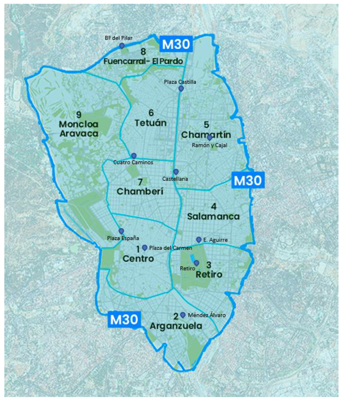
3.1. Location of the Study

The city of Madrid has a population of approximately 3.3 million inhabitants (https://www.ine.es). The most problematic air pollutant in this city is NO₂. The main sources of NO₂ emissions are road traffic (41%), followed by air traffic (22.9%) and heating (21.5%) [40].

Madrid features a well-developed and competitive public transport network, comprising an extensive metro system, eight suburban rail lines, four tram routes and a broad network of urban and suburban bus services [41]. According to the last State of Mobility in the City of Madrid report [42], in 2022, public transport accounted for 24% of total trips; private traffic represented 49% of total trips, of which 79% were made by private vehicles and 21% by professional vehicles; and active mobility made up for 27% of total trips, of which 98% were made on foot and only 2% by bicycle or personal mobility vehicles (PMVs).

The first traffic-restricted area in Madrid was called “Madrid Central” and it comprised the central district, an area of 4.7 km². It was fully operational between March 2019 and July 2020, when it was declared null. After this, a larger LEZ project was developed, called “Madrid ZBE”, which stands for low-emission zone in Spanish, and affects the area limited by the M-30 motorway, Figure 1, that comprises 52 km². Madrid ZBE, from now on Madrid LEZ, has been in operation since December 2021. Starting from January 2022, access for the most polluting vehicles not registered in the municipality of Madrid was prohibited inside the area limited by the M-30 motorway, including petrol cars and vans registered before January 2001 (<EURO 3), and diesel cars and vans registered before January 2006 (<EURO 4). The restricted areas for these vehicles have increased progressively each year. Since January 2025, all these vehicles have been prohibited from accessing public roads throughout the municipality of Madrid, regardless of their registration location. Our study focuses on assessing the impact of the first stage of Madrid LEZ (2022) on air quality.

3.2. Data

There are ten air quality monitoring stations inside the area limited by the M-30, that is, inside Madrid LEZ, seven of them are traffic sites, while the other three are urban background stations.

Table 1. Pollutants monitored at the stations in Madrid (Source: [48]).

Station	Urban Site	Pollutants	Considered in the Study
Barrio del Pilar	Traffic	NOx, O3	√
Castellana	Traffic	NOx, PM10, PM2.5	×
Cuatro Caminos	Traffic	NOx, PM10, PM2.5, BTX	×
Escuelas Aguirre	Traffic	NOx, SO2, CO, PM10, PM2.5, O3, BTX	√
Méndez Álvaro	Background	NOx, PM10, PM2.5	√
Plaza de Castilla	Traffic	NOx, PM10, PM2.5	×
Plaza de España	Traffic	NOx, SO2, CO	×
Plaza del Carmen	Background	NOx, SO2, CO, O3	√
Ramón y Cajal	Traffic	NOx, BTX	√
Retiro	Background	NOx, O3	√

provides an overview of the monitoring sites and the pollutants measured at each location. The hourly concentrations of NO₂, PM₁₀ and PM_2.5, when available, measured at the air quality monitoring stations inside the area limited by the M-30 highway in Madrid were recovered from the European Environment Agency (EEA) using saqgetr package [44] for R [45]. These species were selected as they are typical pollutants emitted by traffic. Most studies analyzing the impact of LEZs focus on NO₂ and/or PM₁₀ and PM_2.5 (e.g., [10,16,18,19,27,39,46]). While SO₂ and O₃ are also considered air pollutants of concern, they were excluded from this study for different reasons. SO₂ is primarily associated with industrial activities. In Spain, its concentrations in urban areas have been steadily declining since 2001 [47], with maximum monthly average values in Madrid remaining at or below 2 µg·${\mathrm{m}}^{-3}$, making it a negligible issue. As for O₃, it is a secondary pollutant whose formation is highly complex and nonlinear, influenced by multiple factors, including transboundary contributions. Due to these characteristics, SO₂ and O₃ are not considered reliable indicators of traffic-related pollution in this study.

Only stations with at least 90% of the hourly data for each year in the period 2015–2022 were further considered, in accordance with the minimum data capture requirements established by Directive 2008/50/EC [49] (Barrio del Pilar, Escuelas Aguirre, Méndez Álvaro, Plaza del Carmen, Ramón y Cajal and Retiro). Daily averages were obtained from the hourly data and fed into the ML algorithms. In this paper, we present the results for the Barrio del Pilar and Méndez Álvaro stations, which represent a traffic site and an urban background site, respectively, where ML algorithms provided accurate predictions. Results for the remaining stations that meet the data coverage criteria are provided in the Supplementary Information file.

Daily meteorological data (maximum and minimum atmospheric pressure, precipitation, wind speed, direction and gusts, and maximum and mean temperatures) were retrieved from the OpenData platform of the Agencia Estatal de Meteorología (AEMET) (https://opendata.aemet.es/ (accessed on 15 December 2024)). Along with meteorological factors, the input variables of the ML algorithms included the date (day and month), the day of the week, biomass combustion episodes and Saharan dust intrusion episodes. Data from both types of episodes were obtained from the Ministerio de Transición Ecológica (https://www.miteco.gob.es/ (accessed on 15 December 2024)) and used in the models as categorical predictors (0: absence of dust intrusion or biomass combustion episode, 1: presence of dust intrusion or biomass combustion episode) to account for emissions different from road traffic.

Traffic intensity data were obtained from the open access data website of the Ayuntamiento de Madrid (https://datos.madrid.es/portal/site/egob (accessed on 15 December 2024)). Traffic data were analyzed locally in areas close to the two selected air quality monitoring stations and, globally, inside the area limited by the M-30 and on the M-30 highway. Traffic data were used to validate our hypothesis of a business-as-usual scenario and were not fed into the models. Finally, the total number of vehicles grouped by fuel category (petrol, diesel and others) in Madrid province were obtained from the website of Dirección General de Tráfico (https://www.dgt.es/menusecundario/dgt-en-cifras/ (accessed on 15 December 2024)).

3.3. Methodology

The methodology used to evaluate the efficiency of the LEZ in each location is based on predicting NO₂, PM₁₀ and PM_2.5 concentrations with three different ML algorithms in a business-as-usual scenario, that is, assuming no changes in the emission patterns. For this purpose, the ML algorithms were trained and validated with data from 2015 to 2018, where no LEZ was in place, and they were used to predict pollutant concentrations in 2022. When accounting for meteorological variables and without other major changes in environmental policies, the observed differences in actual measurements with respect to those predicted by the models can be attributed to the introduction of the LEZ. The relative effect of the LEZ ($R{E}_t$) for a given location is then quantified with each ML algorithm using Equation (1):

$$R{E}_t(\%)=100·{\displaystyle \frac{y_t-y_t^{est}}{y_t^{est}}},$$

(1)

where $y_t^{est}$ is the pollutant concentration estimated on day t with the ML algorithm, and $y_t$ is the actual concentration measured. A similar approach to this one has been used before to estimate the effects of other interventions or events on air quality (e.g., COVID-19) [50].

The ML algorithms used in this study were Random Forest (RF), Ranger and SVM. Random forests consist of an aggregation of tree predictors, where each tree relies on the values of a random vector sampled independently, which has the same distribution across all trees within the forest [51]. Both Random Forest and Ranger are supervised machine learning algorithms based on random forests and they can be used for both classification and regression problems. The main difference between them is that Ranger is a much faster and optimized implementation than the original Random Forest, which is particularly useful when handling high-dimensional data [52]. SVM is a supervised machine learning algorithm that aims at finding the best hyperplane that divides a dataset into classes [53].

These models were chosen because they have been successfully applied in previous studies to predict air pollutant concentrations [54,55,56]. For instance, Random Forest has demonstrated more reliable pollutant concentration predictions compared to gradient boosting and multiple linear regression (MLR) [57], as well as M5P and k-Nearest Neighbors (KNN) [58]. Support Vector Machines (SVMs) have also shown excellent performance in forecasting short-term PM_2.5 concentrations [59], outperforming neural networks in predicting daily maximum O₃ concentrations [60]. More recently, an ensemble model of three decision tree-based algorithms, including Ranger was employed to predict daily NO₂ concentrations in France from 2005 to 2022 [61]. Similarly, extreme air pollution events were identified by modeling PM_2.5 using Ranger [62].

The algorithms Random Forest, Ranger and SVM were implemented in the R libraries randomForest, ranger and e1071, respectively [52,63,64]. To train and validate the algorithms, 80% of the daily data from 2015 to 2018, randomly chosen, was used as the training set; the remaining 20% was used as the validation set. An 80:20 split is a typical data division between the training and validation sets for training ML algorithms used to forecast air pollution [38,65,66,67].

The suitability of the ML algorithms to predict pollutant concentrations was assessed by means of different ways. First of all, the estimated concentrations were plotted against the observed ones, for both the training and the validation sets. These plots show at a glance the goodness of the prediction, so the closer the slope is to 1, the better the prediction. The predictive performance was also evaluated by means of the Root Mean Square Error (RMSE), the Mean Absolute Error (MAE) and the Mean Absolute Percentage Error (MAPE), defined as follows:

$$\begin{array}{ccc}& & RMSE=\sqrt{{\displaystyle \frac{1}{n}\sum _{t=1}^n{(y_t-y_t^{est})}^2}},\hfill \end{array}$$

(2)

$$\begin{array}{ccc}& & {\displaystyle MAE=\frac{1}{n}\sum _{t=1}^n\left|y_t-y_t^{est}\right|,}\hfill \end{array}$$

(3)

$$\begin{array}{ccc}& & {\displaystyle MAPE=\frac{1}{n}\sum _{t=1}^n\left|\frac{y_t-y_t^{est}}{y_t}\right|,}\hfill \end{array}$$

(4)

where $y_t$ is the observed value, $y_t^{est}$ is the estimated value on day t, and n is the number of prediction values. The Pearson coefficient of correlation (r) between predicted and observed values was also calculated for each model:

$$r={\displaystyle \frac{{\displaystyle \sum _{t=1}^n\left(y_t-\overline{y}\right)\left(y_t^{est}-\overline{y^{est}}\right)}}{\sqrt{{\displaystyle \sum _{t=1}^n{\left(y_t-\overline{y}\right)}^2\sum _{t=1}^n{\left(y_t^{est}-\overline{y^{est}}\right)}^2}}}},$$

(5)

where $\overline{y}$ and $\overline{y^{est}}$ are the average observed and estimated values, respectively.

Finally, the relative variation between the daily pollutant concentrations observed for each day of the year 2022 and the average concentration measured on that same day in the period preceding the implementation of the LEZ was computed, given by the following equation:

$$R{V}_t(\%)=100·{\displaystyle \frac{y_t-y_t^{ref}}{y_t^{ref}}},$$

(6)

where $y_t^{ref}$ represents the reference value, which is the average concentration measured during the period prior to the LEZ implementation on day t for each day of the year.

4. Results

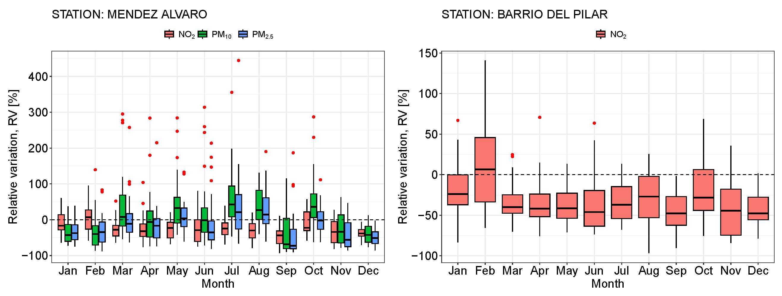
4.1. Concentration of Pollutants in the Period 2015–2022

In this paper, the analysis of NO₂, PM₁₀ and PM_2.5 concentrations, as well as the effect of Madrid LEZ, are shown for two of the stations located inside Madrid LEZ (Méndez Álvaro (background site) and Barrio del Pilar (kerbside site)). The same analysis was carried out for the six stations that met the data quality objective (at least 90% of valid data each year during the studied period), yielding similar results. Results for the other four stations are shown in the Supplementary Information file.

To facilitate comparison of daily concentrations of NO₂, PM₁₀ and PM_2.5 measured from 2015 to 2022, box and whisker plots are provided in Figure 2 for Méndez Álvaro station and Barrio del Pilar station. Four periods can be distinguished in the plots, i.e., (i) before the implementation of any LEZ (2015–2018), (ii) during the existence of Madrid Central (2019), (iii) during the COVID-19 pandemic (2020 and 2021) and (iv) after the implementation of Madrid LEZ (2022).

NO₂ concentrations exhibited a clear annual pattern with lower concentrations in the summer months than in winter for all the studied periods. The monthly median concentration from 2015 to 2018 was higher in every month, except February, compared to the other periods. This can also be observed in Figure 3 for Méndez Álvaro and Barrio del Pilar stations, where the relative difference between the daily concentration of NO₂ in 2022 and the average concentration measured on the same days during the period 2015–2018 was plotted. This suggests that the introduction of the LEZ, along with the mobility restrictions implemented to combat COVID-19, had a significant impact on air quality. However, these assertions must be supported by additional analysis that accounts for the influence of meteorological variables on pollutant concentrations. In this work, this is achieved by incorporating meteorological parameters into the machine learning algorithms used.

PM₁₀ and PM_2.5 were only measured at the Méndez Álvaro station. There was no clear annual pattern followed by the concentrations of particulate matter in the air. Furthermore, there were months in 2022 where the concentrations of particulate matter were higher than in the same months of previous periods. This can be observed more clearly in Figure 3, where RV_t is plotted. Once again, it can be seen that, for NO₂, the monthly medians of the concentrations in 2022 were lower than in the period 2015–2018, except for February; whereas for PM₁₀ and PM_2.5, the monthly medians were higher some months compared to before the LEZ. Atypical values of daily averages of PM₁₀ and PM_2.5 concentrations above 400 µg·${\mathrm{m}}^{-3}$ were registered in March and in the summer months of 2022. It is worth highlighting the significant number of episodes of Saharan dust intrusions that took place in 2022, especially from March to October, which were likely responsible for the high concentrations of PM₁₀ and PM_2.5 recorded. In fact, in March 2022 there were 15 days with dust intrusions from the Sahara that reached the central part of Spain, in May there were 14, in June 11, in July 23, in August 17 and in October 26 days [68].

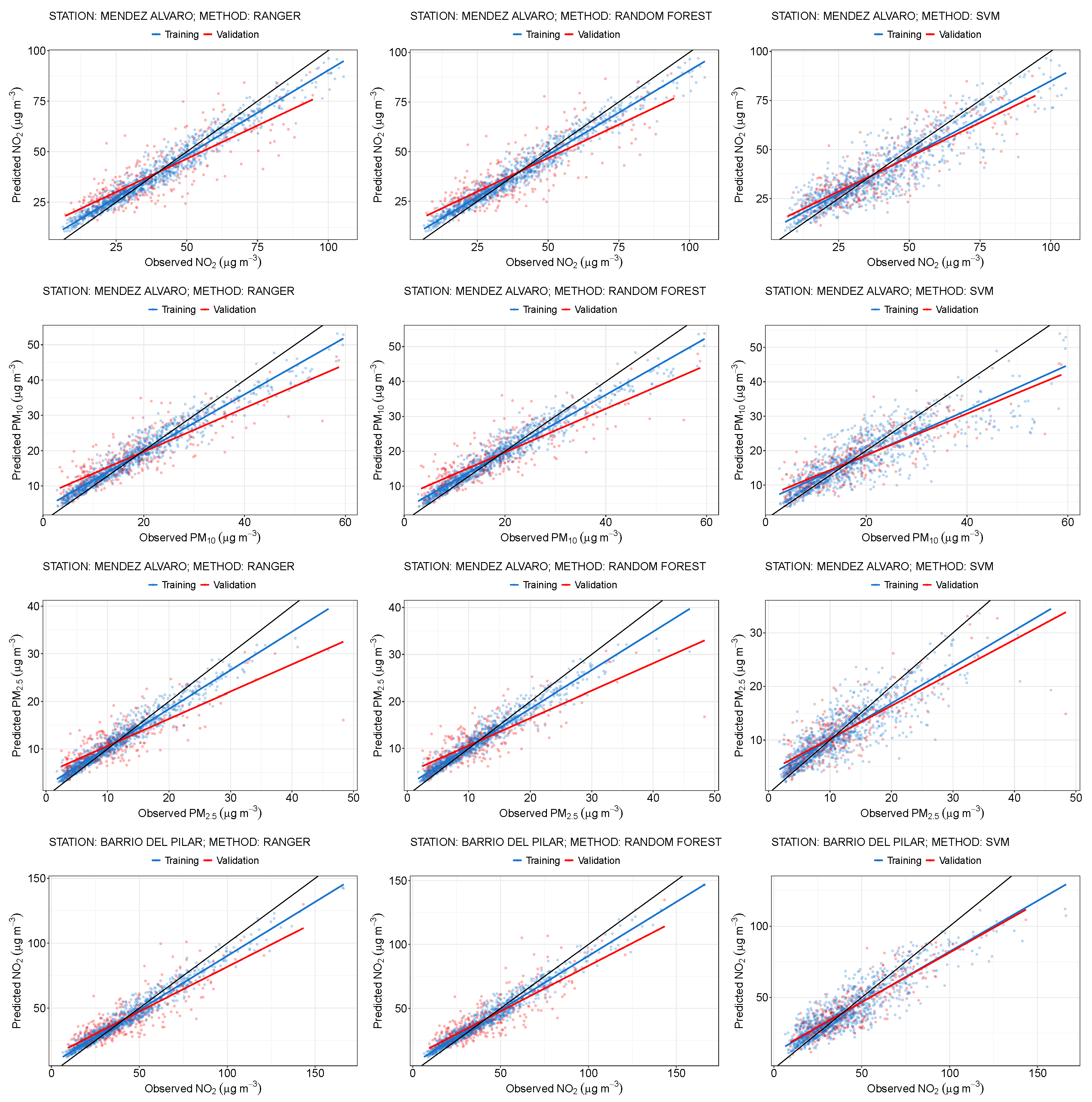
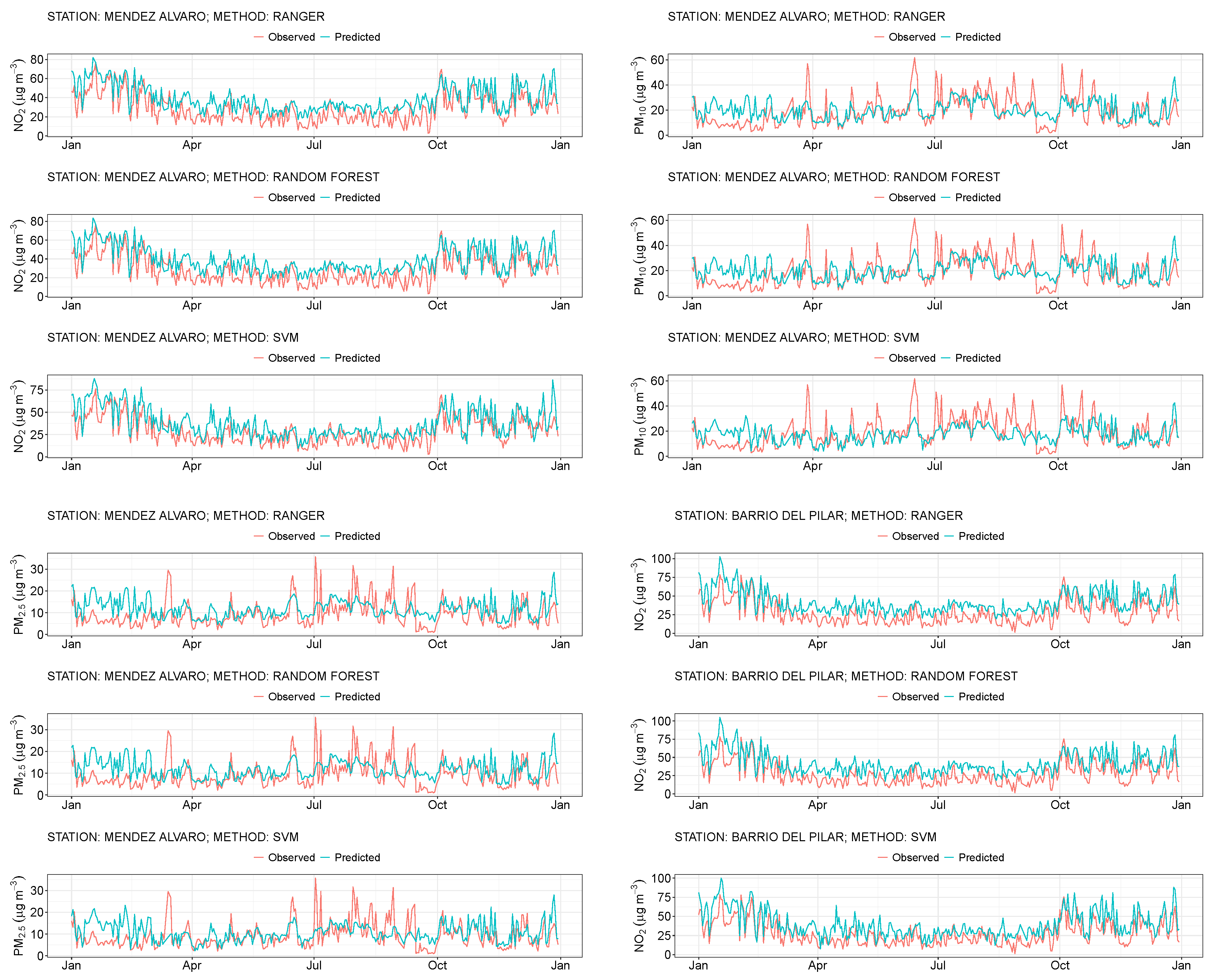
4.2. Validation of ML Algorithms

In

Table 2. Error metrics for the training and validation sets for NO₂, PM₁₀ and PM_2.5 predictions at the Méndez Álvaro station and for NO₂ predictions at the Barrio del Pilar station.

Méndez Álvaro Station
Polluant	Model	Set	MAE ($\mathrm{\mu }\mathrm{g}{\mathrm{m}}^{-\mathbf{3}}$)	MAPE	RMSE ($\mathrm{\mu }\mathrm{g}{\mathrm{m}}^{-\mathbf{3}}$)	${\mathit{r}}^{\mathbf{2}}$
NO2	RF	Training	3.58	0.12	4.61	0.96
	Ranger	Training	3.73	0.13	4.79	0.95
	SVM	Training	6.18	0.20	8.51	0.82
	RF	Validation	8.38	0.26	10.60	0.68
	Ranger	Validation	8.41	0.26	10.62	0.68
	SVM	Validation	7.93	0.24	10.17	0.71
PM10	RF	Training	2.04	0.13	2.82	0.94
	Ranger	Training	2.10	0.14	2.91	0.94
	SVM	Training	3.56	0.21	5.48	0.74
	RF	Validation	4.29	0.32	5.64	0.70
	Ranger	Validation	4.28	0.32	5.62	0.71
	SVM	Validation	4.20	0.29	5.81	0.69
PM2.5	RF	Training	1.25	0.14	1.77	0.94
	Ranger	Training	1.29	0.14	1.81	0.94
	SVM	Training	2.23	0.23	3.35	0.74
	RF	Validation	2.85	0.32	3.95	0.65
	Ranger	Validation	2.85	0.33	4.00	0.65
	SVM	Validation	2.76	0.31	4.03	0.63
Barrio del Pilar Station
Polluant	Model	Set	MAE ($\mathrm{\mu }\mathrm{g}{\mathrm{m}}^{-\mathbf{3}}$)	MAPE	RMSE ($\mathrm{\mu }\mathrm{g}{\mathrm{m}}^{-\mathbf{3}}$)	${\mathit{r}}^{\mathbf{2}}$
NO2	RF	Training	4.07	0.13	5.39	0.96
	Ranger	Training	4.25	0.13	5.62	0.96
	SVM	Training	7.29	0.21	10.32	0.81
	RF	Validation	9.36	0.26	11.88	0.70
	Ranger	Validation	9.28	0.26	11.80	0.71
	SVM	Validation	8.56	0.23	11.13	0.74

, the summary of the prediction error metrics obtained for the training and validation sets obtained with each ML model for Méndez Álvaro and Barrio del Pilar stations, respectively, are shown.

For both stations, the models exhibited strong performance on the training sets ($r^2$ > 0.7), with RF and Ranger demonstrating the best adjustments and lowest errors. On the validation sets, the error metrics were slightly higher and $r^2$ values were lower compared to the training sets, yet they remained above 0.65 in every case. This indicates that the models captured the behavior of the studied air pollutants reasonably well. Notably, SVM yielded superior metrics for NO₂ with the validation sets, while RF and Ranger outperformed for PM₁₀ and PM_2.5 in both training and validation sets.

The distributions of errors are shown in Figures S8 and S9 in the Supplementary Information file. The error histograms exhibit a bell-shaped distribution, with the highest frequencies observed around zero. Errors are represented in three different colors, depending on whether the observed concentration is low, medium or high. Different concentration ranges have been established for each pollutant based on the observed average concentrations. The histograms show that all three models tend to overfit at low concentrations and underfit at high concentrations. Overall, there is a slight tendency toward overfitting.

An analysis of the feature importance was also performed (Figures S11 and S12 in the Supplementary Information file). For NO₂, all three models identified average wind speed as one of the three most important features. For Ranger and Random Forest, wind gusts were also highly important, along with the month and the day of the week, respectively. In the case of SVM, minimum and maximum temperatures had a significant impact on the model’s outputs. Regarding PM₁₀, dust intrusions were the most important feature when using Ranger and Random Forest and the third most important when using SVM. Wind gusts, wind direction, and maximum and average temperatures were also influential variables. Similarly, dust intrusions played a key role in predicting PM_2.5 concentrations with Ranger and Random Forest; however, this feature was not among the three most important ones when forecasting with SVM. Temperature and wind speed have previously been identified as key factors in forecasting air pollution using machine learning algorithms [69,70].

Figure 4 depicts the predicted values versus observed values for the training sets (blue) and the validation sets (red) for pollutants measured at Méndez Álvaro and Barrio del Pilar. The black line represents the identity line (y = x), where closer alignment between the red and blue lines indicates better model performance. These figures revealed higher dispersion of values with the SVM model; however, this model exhibited more consistent behavior between the training and validation sets (with very similar slopes of the blue and red lines). Additionally, it is evident that the models performed more effectively with NO₂ compared to the other pollutants. Nevertheless, given the overall satisfactory predictions, all models were utilized to forecast NO₂, PM₁₀ and PM_2.5 concentrations in the immediacy of each air pollution monitoring station in 2022 under a business-as-usual scenario to evaluate the effect of Madrid LEZ.

The predicted and observed concentrations of NO₂, PM₁₀ and PM_2.5 in Méndez Álvaro in 2022 are shown in Figure 5. The predicted concentrations for NO₂ exceeded the observed values in many cases. All three models effectively captured the daily variation in NO₂ concentrations, which were particularly evident in the latter months of the year. As seen in Figure 3, NO₂ concentrations were notably lower in 2022 compared to the period spanning from 2015 to 2018. Given this context, it is reasonable that the three models predicted NO₂ concentrations to be higher than what was actually observed. Regarding PM_2.5 and PM₁₀, there was a notable discrepancy between the predicted concentrations and the observed values on many days, even though the models included a categorical variable for biomass combustion episodes and Saharan dust intrusions. Specifically, the trend of the predictions appeared smoother than that of the observed concentrations, which is particularly evident from April to October, coinciding with peak values associated with dust intrusions.

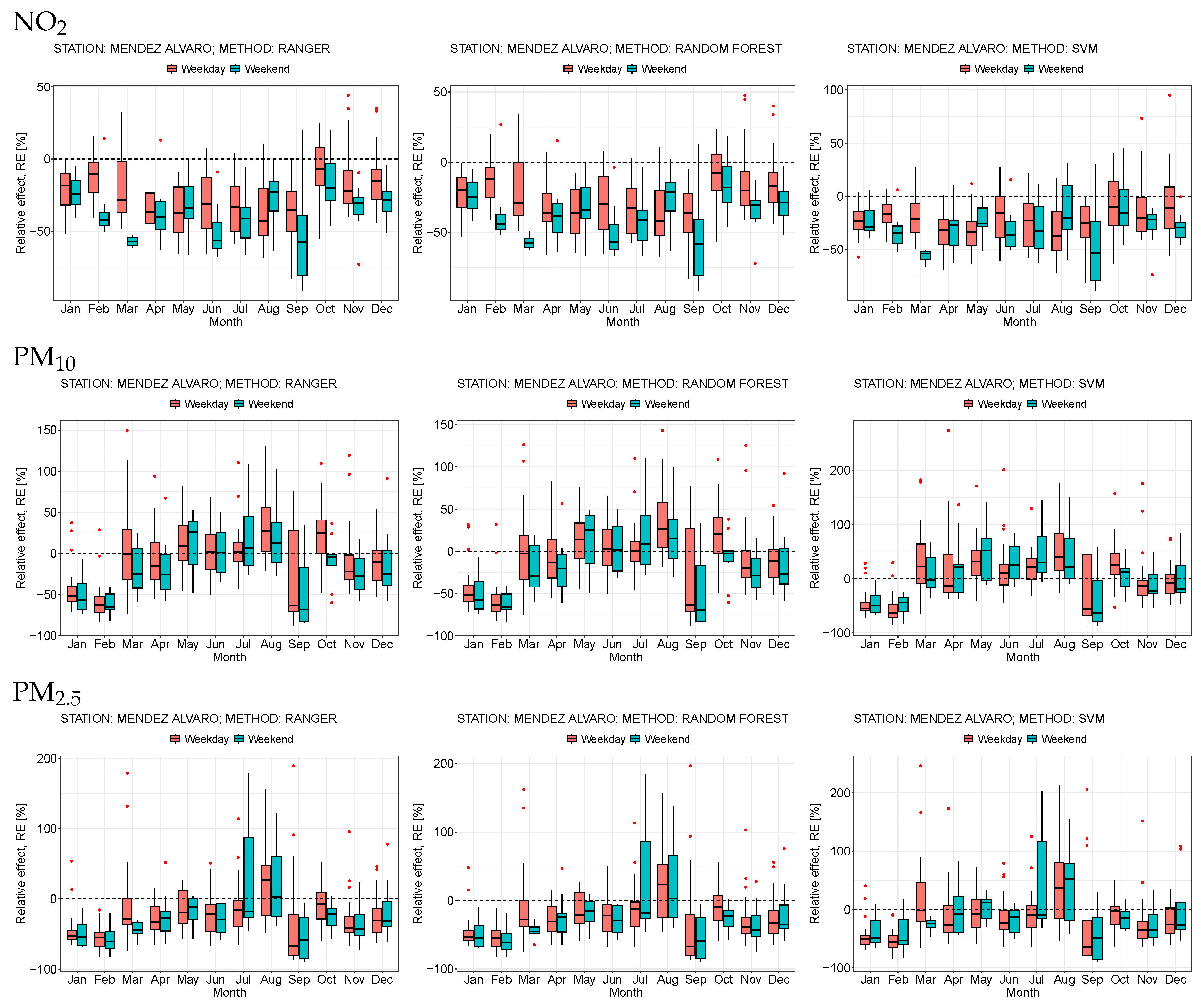
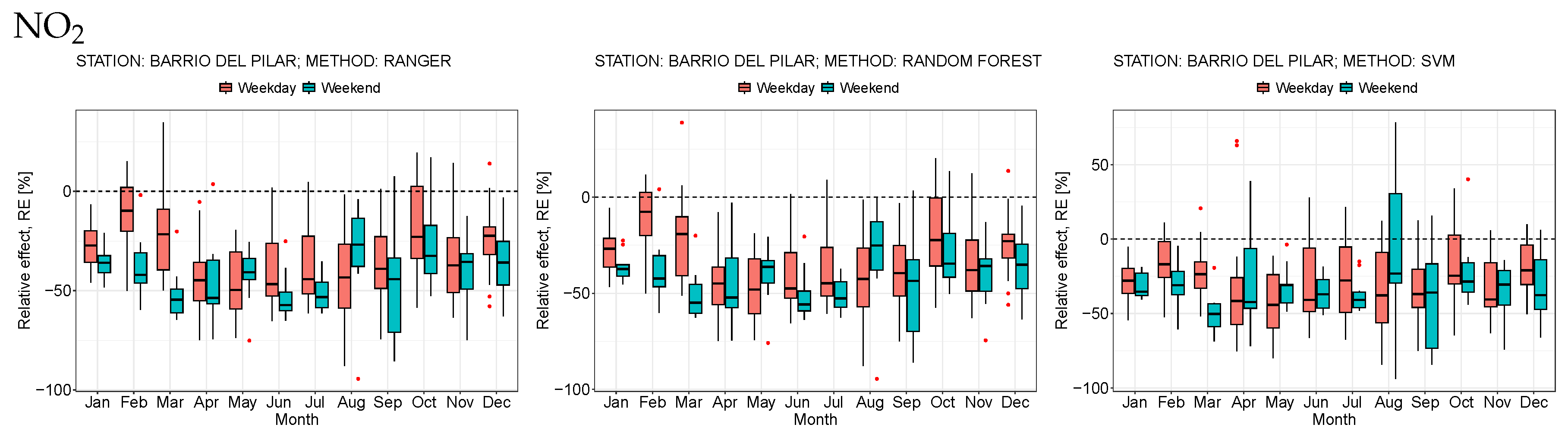
4.3. Effect of Madrid LEZ on the Air Quality

The relative effect of Madrid LEZ on the air quality was calculated for each monitoring site and each pollutant using Equation (1), distinguishing among weekdays and weekends.

The relative effect of the LEZ on NO₂ concentrations turned out to be very similar at both monitoring sites. In Figure 6 and Figure 7, it can be seen that the NO₂ reductions were higher on weekends than on weekdays for most of the months. In general, the measured concentrations of NO₂ were lower than those predicted by the models. Further, all three models provide similar results, specially RF and Ranger, whereas the reductions in NO₂ concentrations calculated with SVM are slightly lower than with the other two models. The descriptive statistics of the relative effects are shown in

Table 3. Summary statistics of daily relative effects after implementing the LEZ in 2022 according to the prediction models for NO₂, PM₁₀ and PM_2.5 at the Méndez Álvaro station and for NO₂ at the Barrrio del Pilar station.

Méndez Álvaro Station
Polluant	Model	Mean	Sd	Min	Max	Q1	Q2	Q3
NO2	RF	−27.23	23.40	−91.76	47.66	−42.65	−29.72	−11.08
	Ranger	−27.29	23.03	−91.47	44.19	−42.78	−29.78	−11.48
	SVM	−22.85	25.34	−89.04	94.87	−38.79	−25.95	−8.21
PM10	RF	−7.50	44.91	−88.51	143.18	−42.13	−10.19	19.92
	Ranger	−7.40	45.00	−88.50	149.51	−41.82	−10.39	21.56
	SVM	8.68	58.21	−87.52	273.48	−33.07	0.51	37.47
PM2.5	RF	−20.59	45.55	−89.29	196.65	−50.51	−30.83	−4.60
	Ranger	−20.74	45.19	−89.32	189.42	−49.92	−30.64	−4.85
	SVM	−9.71	54.38	−89.23	246.18	−46.61	−20.66	9.30
Barrrio del Pilar Station
Polluant	Model	Mean	Sd	Min	Max	Q1	Q2	Q3
NO2	RF	−34.96	21.13	−94.58	38.83	−50.10	−36.67	−20.77
	Ranger	−34.98	21.29	−94.42	34.58	−50.99	−36.06	−20.22
	SVM	−29.25	24.63	−93.95	78.22	−45.70	−31.21	−15.11

for 2022. Depending on the model, the annual average reduction in NO₂ varies from −22.9 to −27.3%, approximately, in Méndez Álvaro station and from −29.3 to −35% in Barrio del Pilar.

Comparing these results with other studies is not straightforward, as LEZ policies vary across countries. For instance, while most LEZs operate continuously, some are only in effect on weekdays or during specific time slots. Additionally, certain LEZs target only diesel vehicles, whereas others also impose restrictions on some petrol vehicles. Moreover, some LEZs allow access to polluting vehicles upon payment of a fee [71]. Differences in cities’ main emission sources, meteorological conditions and overlapping policies, along with the diverse methodologies used to assess the impact of LEZs on air pollution, further complicate comparisons. In any case, our findings on NO₂ reductions are consistent with those reported by other authors using a DID approach. For example, Prieto-Rodriguez et al. [26] found a 19% reduction in NO₂ concentrations for the London ULEZ; Salas et al. [24] reported similar reductions in Madrid Central—a special protection low-emission zone within Madrid ZBE—ranging from 23% to 34% in 2019; and Park and Lim [27] observed a 17.3% decrease in Seoul in 2020. However, other studies have reported lower NO₂ reductions using different methodologies. For instance, Hajmmohammadi and Heydecker [21] found a 12% NO₂ reduction in London using a state-space intervention method. Park and Tauri [22] reported an 11.6% decrease in Seoul and Ma et al. [8] observed a 3% decrease in London, both employing a regression discontinuity design.

When analyzing the relative effect of the LEZ on PM₁₀ and PM_2.5 it is not clear whether there is a positive impact on air quality (Figure 6). In fact, approximately half of the months in 2022 show relative effects with positive medians, indicating that the observed values were higher than those predicted by the models. Slightly better results are obtained with PM_2.5 than with PM₁₀. Furthermore, the observed values of PM_2.5 and PM₁₀ (represented by the red lines in Figure 5) do not exhibit any discernible annual or daily pattern that could be attributed to traffic emissions or their dispersion. This complicates their utility as proper tracers for assessing the effectiveness of air pollution mitigation strategies using our approach, particularly in areas where emissions from natural sources play a significant role.

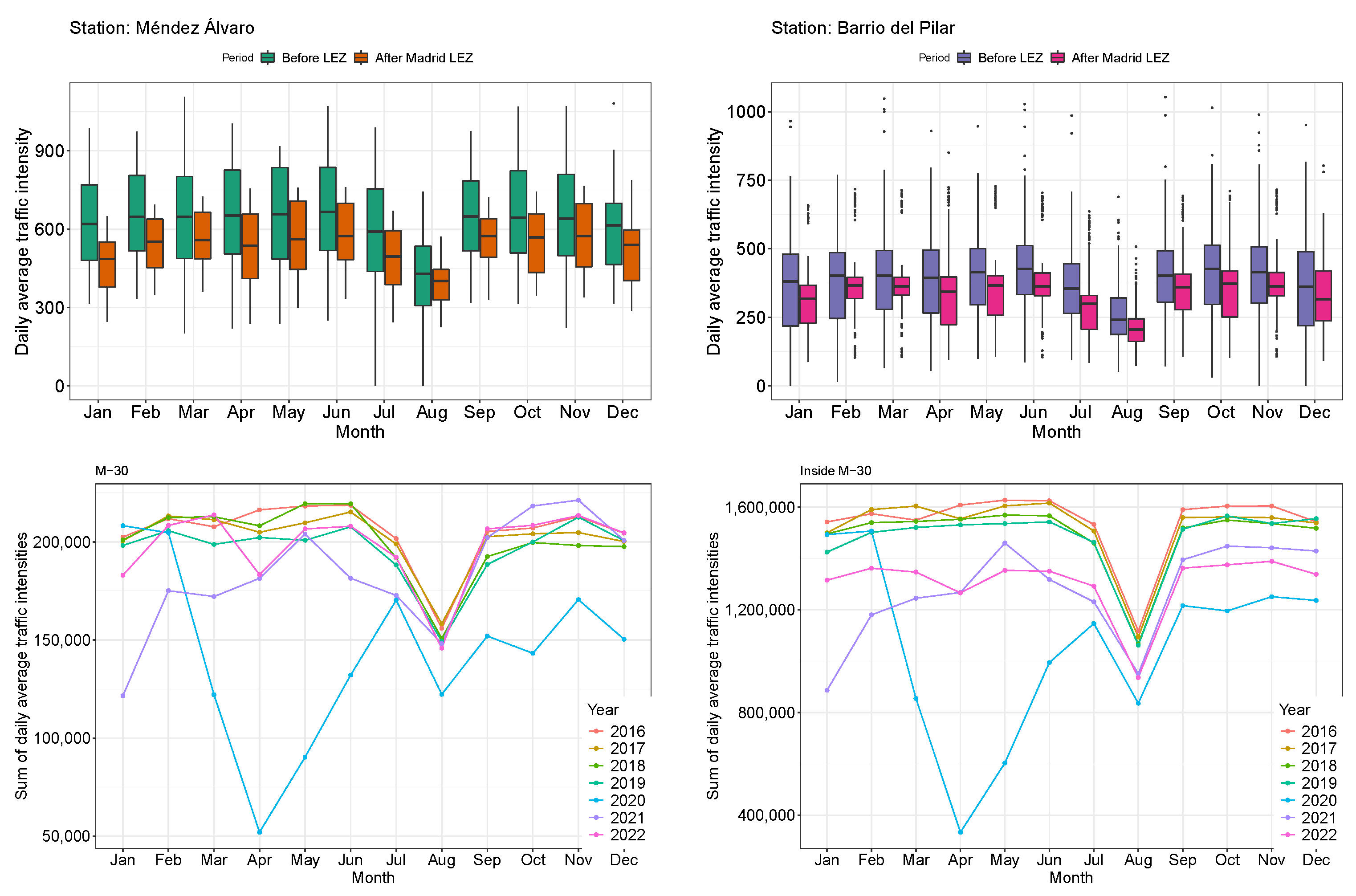
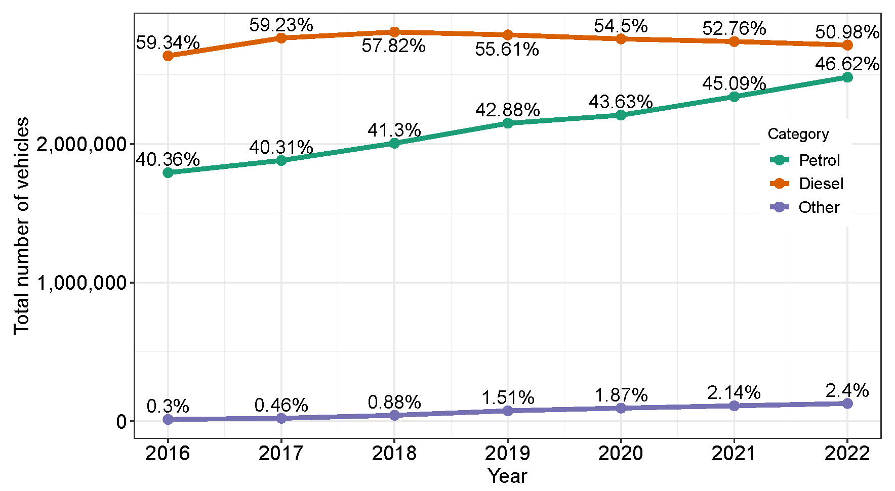
4.4. Analysis of Traffic Volume

Traffic data were analyzed both locally and globally to assess whether the LEZ may have contributed to mobility changes in the capital of Spain. Local traffic in the vicinity of the Méndez Álvaro air quality station was studied using data from a permanent traffic counter located nearby. For the Barrio del Pilar air quality station, data from the two nearest permanent traffic counters, located 700 and 900 m apart, respectively, were utilized. Additionally, traffic within the inner ring of the M-30 motorway and on the M-30 itself was examined (Figure 8).

It is worth noting that within the M-30 and particularly in the vicinity of the monitored air quality stations, the average daily traffic volume in 2022 was significantly lower compared to the period from 2016 to 2018. The years 2020 and 2021 were notably atypical due to mobility restrictions imposed following the COVID-19 pandemic. When analyzing traffic volume on the M-30 motorway, the differences between 2022 and the years 2016 to 2019 were less pronounced. It is important to remember that in 2022, the most polluting vehicles were prohibited within the M-30, except on the actual M-30 motorway. These results suggest a reduction in traffic volume as a result of the LEZ.

5. Discussion

Investment in and promotion of public transportation, active modes of mobility, or the prohibition of entry into city centers for the most polluting vehicles are among the most popular mitigation strategies that public authorities have been adopting in recent years to combat air pollution in urban areas. Estimating the effectiveness of the implemented measures, however, is complex due to the simultaneous contributions and the combined effects of different policies to air quality [72].

In this paper, a simple and low-cost methodology is proposed to assess the efficiency of Madrid LEZ established in 2021. Due to the coincidence of the initiation of this LEZ and the measures still in place to curb the COVID-19 pandemic, the analysis was conducted for the year 2022, in comparison to the period 2015–2018, prior to the existence of any LEZ in Madrid and the pandemic.

The analysis of traffic volume inside the LEZ from 2015 to 2022 revealed a significant reduction in the years 2020, 2021 and 2022. While 2020 marked the onset of the COVID-19 pandemic and 2021 saw some mobility restrictions to curb the spread of the virus, 2022 experienced a return to normalcy with no pandemic-related mobility constraints, and Madrid LEZ was also operational. Consequently, this year was highly suitable for this analysis.

ML algorithms provided promising results in predicting air pollutant concentrations by incorporating seasonal and meteorological factors; however, a slight overestimation of concentrations was detected, especially at low concentration levels. While traffic volume was analyzed in the paper to support this discussion, it was not included as an input in the models. This decision was made because obtaining traffic data with the necessary resolution for model input can be challenging, and one of the key premises of this study was to develop a methodology that was easy to apply. Additionally, the approach adopted in this paper (business-as-usual scenario) assumes no changes in emission patterns between the years used to train the models and the year for which pollutant concentrations were predicted (2022). Therefore, incorporating emissions as inputs into the models would not be meaningful.

The decline in traffic volume within the area limited by the M-30 motorway in 2022, but not on the M-30 itself, suggests that it was likely attributable to the presence of the LEZ rather than significant behavioral changes spurred by the pandemic (e.g., a substantial increase in telecommuting compared to pre-COVID-19 times). In fact, recent works have established no associations between telework and traffic reduction or air quality improvements in Madrid [73,74]. The reduction in traffic volume was well reflected in the concentrations of NO₂ in the air in 2022, which were significantly lower than during the period 2015–2018. Indeed, all three ML models predicted higher NO₂ concentrations in 2022 under a business-as-usual scenario. Thus, it appears that the reduction in traffic volume directly impacted the concentrations of this pollutant. Moreover, the air surrounding the Barrio del Pilar station experienced the most significant improvement from this reduction, given its kerbside location. This can be confirmed by comparing the relative effects of the LEZ observed for this station with those for Méndez Álvaro (Table 3).

The composition of Madrid’s vehicle fleet was also analyzed from 2016 to 2022 to assess its impact on the reduction in pollutant concentrations, Figure 9. In recent years, there has been an increase in the number of cleaner vehicles (electric, hybrid, etc.), which might suggest they played a key role in the reduction in NO₂ concentrations. While it is true that the registration of greener vehicles is growing each year, their share of the total fleet remains relatively small. For example, in 2022, vehicles other than petrol and diesel accounted for only 2.40% of the total fleet in the province of Madrid.

Reductions in concentrations of PM₁₀ and PM_2.5 were not observed, as noted by other authors [15,50], highlighting the fact that particles originate from various sources besides traffic, such as construction, residential heating, or natural sources. In fact, the highest levels of Sahara dust in Europe are found in Spain and Italy, decreasing from South to North of Europe [75]. The slightly better results for PM_2.5 compared to PM₁₀ were likely due to the higher dependence of PM₁₀ on the occurrence of natural dust intrusion events [76]. While establishing methodologies to evaluate the effectiveness of mitigation strategies on air quality is important, it is also crucial to consider the unique characteristics of each city. For example, particulate matter should not be relied upon as the sole marker of traffic pollution in Southern European countries that experience frequent dust intrusions from Africa unless this contribution is properly assessed [77,78]. Natural events are likely responsible for the differences observed in our study regarding the effect of LEZs on particle concentrations in air, as other studies that do recognize an improvement in particulate matter concentrations were conducted in Northern European countries, such as the United Kingdom and Germany [6,7], or used other methodologies that, directly or indirectly, accounted for other sources of particulate matter.

In any case, the implementation of Madrid LEZ certainly enhanced air quality. Considering that restrictions were set to intensify progressively (for instance, from January 2024, circulation of the most polluting vehicles was restricted through all public and urban roads in the whole municipality of Madrid), we anticipate additional improvements in air quality, particularly in NO₂ concentrations. The ongoing shift toward greener vehicles each year will likely further enhance this improvement.

6. Considerations and Future Work

Business-as-usual approaches rely on the assumption that existing trends will continue over time without significant changes. This serves as a reference scenario to assess the impact of new measures or policies. In this study, we assumed that emissions in Madrid in 2022 were similar to those in previous years (2015–2019). However, 2022 saw a significant decrease in traffic intensity, which we attributed to the implementation of Madrid LEZ.

A key limitation of this approach is the presence of overlapping policies that may have been introduced alongside the LEZ. In such cases, isolating the specific effects of the LEZ from other measures becomes challenging. For example, while the share of electric vehicles in Madrid’s fleet during the study period was negligible, the ongoing shift toward greener vehicles could pose challenges for applying this method in future years. One way to address this issue would be to incorporate new input variables into the models, accounting for the number of vehicles based on their environmental classification. The same principle applies to other concurrent policies, such as public transport subsidies, which would need to be considered to properly isolate the LEZ’s impact, though this would inevitably add complexity to the models.

Another limitation of our approach is the assumption that emission sources other than road traffic remain constant or follow similar annual patterns throughout the study period. In Madrid, efforts to improve air quality have included subsidies for replacing coal-based domestic heating systems and reducing the use of diesel heating, which may impact NO₂ concentrations. However, a recent study projecting NO₂ concentration changes in Madrid in a scenario where existing domestic heating boilers were replaced with more efficient ones found negligible impacts from this measure [79].

A major drawback of our methodology is that it excludes PM₁₀ and PM_2.5 as reliable indicators of LEZ effectiveness due to the random nature of dust intrusion events. Additionally, a significant fraction of particulate matter originates from secondary formation processes [27] and resuspended soil particles [77], limiting the applicability of our approach even in cities unaffected by natural sources.

Our approach could be applied to assess the impact of LEZs on NO₂ concentrations in other cities, if emission patterns from non-traffic sources remain stable and no other concurrent policies are introduced. If additional policies are implemented, their contributions would need to be accounted for in the models.

Finally, it is worth noting that alternative methodologies, also based on machine learning algorithms, could incorporate traffic data into the models. In such cases, a BAU scenario would no longer be relevant. These models would require additional input data and processing time but comparing their results with those obtained in this study could help determine the most effective methodology for assessing LEZ benefits. Additionally, state-of-the-art machine learning algorithms may offer more accurate forecasts and help reduce the overestimation observed in this study. A comparative analysis of different approaches, including DID, applied to the same LEZ case study would provide valuable insights and contribute meaningfully to this research field. Future work should also analyze the extent of the influence of Madrid LEZ on air pollution improvement once all planned restrictions are in place.

7. Conclusions

The methodology applied in this paper establishes the key assumption of similar emissions in 2022 within Madrid LEZ as in the period 2015–2018 (pre-LEZ). Through the use of ML algorithms, the prediction of NO₂, PM₁₀ and PM_2.5 concentrations in 2022 is conducted under a business-as-usual scenario in two locations (suburban and kerbside) inside Madrid LEZ, considering seasonal and meteorological factors as features of the models. The differences between predicted concentrations and observations were attributed to the actual reduction in traffic volume, likely motivated by the LEZ. The predictions of the models were acceptable in every case; however, they failed to predict sudden fluctuations of particulate matter, despite incorporating dust intrusions as a categorical feature.

No improvement in air quality due to the LEZ regarding particulate matter was observed. On the contrary, observed NO₂ concentrations were below those predicted by the models, and they were also significantly lower than concentrations measured during the period 2015–2018. Traffic volume was also analyzed during the years spanning from 2016 to 2022, and a significant decrease in 2022 within the LEZ was observed. All of this seems to indicate that the LEZ contributed to improve the air quality of Madrid in terms of NO₂, due to the subsequent reduction in traffic; however, the natural contributions to particulate matter concentrations preclude them from being used as traffic pollution tracers in cities that suffer from dust intrusions using our approach. Construction activities, biomass combustion, secondary processes and soil resuspension can also contribute to particulate matter concentrations. Therefore, these sources should be quantified if a BAU approach like ours is to be applied, and should be addressed, if necessary, for further reductions in PM₁₀ and PM_2.5 levels.

References

1. Manisalidis, I.; Stavropoulou, E.; Stavropoulos, A.; Bezirtzoglou, E. Environmental and Health Impacts of Air Pollution: A Review. Front. Public Health 2020, 8, 14. [Google Scholar] [CrossRef] [PubMed]
2. Statista. Total Number of Declared Low-Emission Zones (LEZs) in Europe in 2022, with a Projection for 2025, by Country. 2023. Available online: https://www.statista.com/statistics/1321264/low-emission-zones-europe-by-country/ (accessed on 15 January 2024).
3. Gobierno de España. Real Decreto 1052/2022, de 27 de Diciembre, por el que se Regulan las Zonas de Bajas Emisiones. 2022. Available online: https://www.boe.es/eli/es/rd/2022/12/27/1052 (accessed on 15 January 2024).
4. Boogaard, H.; Janssen, N.A.; Fischer, P.H.; Kos, G.P.; Weijers, E.P.; Cassee, F.R.; van der Zee, S.C.; de Hartog, J.J.; Meliefste, K.; Wang, M.; et al. Impact of low emission zones and local traffic policies on ambient air pollution concentrations. Sci. Total Environ. 2012, 435-436, 132–140. [Google Scholar] [CrossRef] [PubMed]
5. Sánchez, J.M.; Ortega, E.; López-Lambas, M.E.; Martín, B. Evaluation of emissions in traffic reduction and pedestrianization scenarios in Madrid. Transp. Res. Part D Transp. Environ. 2021, 100, 103064. [Google Scholar] [CrossRef]
6. Ellison, R.B.; Greaves, S.P.; Hensher, D.A. Five years of London’s low emission zone: Effects on vehicle fleet composition and air quality. Transp. Res. Part D Transp. Environ. 2013, 23, 25–33. [Google Scholar] [CrossRef]
7. Gu, J.; Deffner, V.; Küchenhoff, H.; Pickford, R.; Breitner, S.; Schneider, A.; Kowalski, M.; Peters, A.; Lutz, M.; Kerschbaumer, A.; et al. Low emission zones reduced PM10 but not NO2 concentrations in Berlin and Munich, Germany. J. Environ. Manag. 2022, 302, 114048. [Google Scholar] [CrossRef]
8. Ma, L.; Graham, D.J.; Stettler, M.E.J. Has the ultra low emission zone in London improved air quality? Environ. Res. Lett. 2021, 16, 124001. [Google Scholar] [CrossRef]
9. Bishop, H.F.J.; Bornioli, A. Effectiveness of London’s Ultra Low Emission Zone in Reducing Air Pollution: A Pre- and Post-Comparison of NO2 and PM10 Levels. J. Environ. Health 2021, 85, 16–23. [Google Scholar]
10. Gómez-Losada, Á.; Pires, J.C. Air quality assessment during the low emission zone implementation in Madrid (Spain). Urban Clim. 2024, 55, 101995. [Google Scholar] [CrossRef]
11. Rodriguez-Rey, D.; Guevara, M.; Linares, M.P.; Casanovas, J.; Armengol, J.M.; Benavides, J.; Soret, A.; Jorba, O.; Tena, C.; García-Pando, C.P. To what extent the traffic restriction policies applied in Barcelona city can improve its air quality? Sci. Total Environ. 2022, 807, 150743. [Google Scholar] [CrossRef]
12. Dias, D.; Tchepel, O.; Antunes, A.P. Integrated modelling approach for the evaluation of low emission zones. J. Environ. Manag. 2016, 177, 253–263. [Google Scholar] [CrossRef]
13. Holnicki, P.; Kałuszko, A.; Nahorski, Z. A Projection of Environmental Impact of a Low Emission Zone Planned in Warsaw, Poland. Sustainability 2023, 15, 16260. [Google Scholar] [CrossRef]
14. Velásquez, A.R.; Guevara, M.; Armengol, J.M.; Rodríguez-Rey, D.; Mueller, N.; Cirach, M.; Khomenko, S.; Nieuwenhuijsen, M. Health impact assessment of urban and transport developments in Barcelona: A case study. Health Place 2025, 91, 103406. [Google Scholar] [CrossRef] [PubMed]
15. Fabregat, A.; Vernet, A.; Vernet, M.; Vázquez, L.; Ferré, J.A. Using Machine Learning to estimate the impact of different modes of transport and traffic restriction strategies on urban air quality. Urban Clim. 2022, 45, 101284. [Google Scholar] [CrossRef]
16. Ferreira, F.; Gomes, P.; Tente, H.; Carvalho, A.; Pereira, P.; Monjardino, J. Air quality improvements following implementation of Lisbon’s Low Emission Zone. Atmos. Environ. 2015, 122, 373–381. [Google Scholar] [CrossRef]
17. Santos, F.M.; Gómez-Losada, Á.; Pires, J.C. Impact of the implementation of Lisbon low emission zone on air quality. J. Hazard. Mater. 2019, 365, 632–641. [Google Scholar] [CrossRef] [PubMed]
18. Lebrusán, I.; Toutouh, J. Using Smart City Tools to Evaluate the Effectiveness of a Low Emissions Zone in Spain: Madrid Central. Smart Cities 2020, 3, 456–478. [Google Scholar] [CrossRef]
19. Font, A.; Guiseppin, L.; Blangiardo, M.; Ghersi, V.; Fuller, G.W. A tale of two cities: Is air pollution improving in Paris and London? Environ. Pollut. 2019, 249, 1–12. [Google Scholar] [CrossRef]
20. Grange, S.K.; Carslaw, D.C. Using meteorological normalisation to detect interventions in air quality time series. Sci. Total Environ. 2019, 653, 578–588. [Google Scholar] [CrossRef]
21. Hajmohammadi, H.; Heydecker, B. Evaluation of air quality effects of the London ultra-low emission zone by state-space modelling. Atmos. Pollut. Res. 2022, 13, 101514. [Google Scholar] [CrossRef]
22. Park, D.; Tarui, N. The Effect of Diesel Vehicle Regulation on Air Quality in Seoul: Evidence from Seoul’s Low Emission Zone. Sustainability 2024, 16, 9573. [Google Scholar] [CrossRef]
23. Rybarczyk, Y.; Zalakeviciute, R. Regression Models to Predict Air Pollution from Affordable Data Collections; IntechOpen: Rijeka, Croatia, 2017; Chapter 2. [Google Scholar] [CrossRef]
24. Salas, R.; Perez-Villadoniga, M.J.; Prieto-Rodriguez, J.; Russo, A. Were traffic restrictions in Madrid effective at reducing NO2 levels? Transp. Res. Part D Transp. Environ. 2021, 91, 102689. [Google Scholar] [CrossRef]
25. Zhai, M.; Wolff, H. Air pollution and urban road transport: Evidence from the world’s largest low-emission zone in London. Environ. Econ. Policy Stud. 2021, 23, 721–748. [Google Scholar] [CrossRef]
26. Prieto-Rodriguez, J.; Perez-Villadoniga, M.J.; Salas, R.; Russo, A. Impact of London Toxicity Charge and Ultra Low Emission Zone on NO2. Transp. Policy 2022, 129, 237–247. [Google Scholar] [CrossRef]
27. Park, D.; Lim, B.I. The effect of the ultra-low emission zone on PM2.5 concentration in Seoul, South Korea. Atmos. Environ. 2025, 340, 120908. [Google Scholar] [CrossRef]
28. Du, M.; Zhang, J.; Hou, X. Decarbonization like China: How does green finance reform and innovation enhance carbon emission efficiency? J. Environ. Manag. 2025, 376, 124331. [Google Scholar] [CrossRef] [PubMed]
29. Apte, J.S.; Messier, K.P.; Gani, S.; Brauer, M.; Kirchstetter, T.W.; Lunden, M.M.; Marshall, J.D.; Portier, C.J.; Vermeulen, R.C.; Hamburg, S.P. High-Resolution Air Pollution Mapping with Google Street View Cars: Exploiting Big Data. Environ. Sci. Technol. 2017, 51, 6999–7008. [Google Scholar] [CrossRef] [PubMed]
30. Moral-Carcedo, J. Dissuasive effect of low emission zones on traffic: The case of Madrid Central. Transportation 2022, 51, 25–49. [Google Scholar] [CrossRef]
31. Lurkin, V.; Hambuckers, J.; van Woensel, T. Urban low emissions zones: A behavioral operations management perspective. Transp. Res. Part A Policy Pract. 2021, 144, 222–240. [Google Scholar] [CrossRef]
32. Ceccato, R.; Rossi, R.; Gastaldi, M. Low emission zone and mobility behavior: Ex-ante evaluation of vehicle pollutant emissions. Transp. Res. Part A Policy Pract. 2024, 185, 104101. [Google Scholar] [CrossRef]
33. Gonzalez, J.N.; Gomez, J.; Vassallo, J.M. Are low emission zones and on-street parking management effective in reducing parking demand for most polluting vehicles and promoting greener ones? Transp. Res. Part A Policy Pract. 2023, 176, 103813. [Google Scholar] [CrossRef]
34. Lee, M.; Lin, L.; Chen, C.Y.; Tsao, Y.; Yao, T.H.; Fei, M.H.; Fang, S.H. Forecasting Air Quality in Taiwan by Using Machine Learning. Sci. Rep. 2020, 10, 4153. [Google Scholar] [CrossRef] [PubMed]
35. Liu, Y.; Wang, P.; Li, Y.; Wen, L.; Deng, X. Air quality prediction models based on meteorological factors and real-time data of industrial waste gas. Sci. Rep. 2022, 12, 9253. [Google Scholar] [CrossRef] [PubMed]
36. Samad, A.; Garuda, S.; Vogt, U.; Yang, B. Air pollution prediction using machine learning techniques—An approach to replace existing monitoring stations with virtual monitoring stations. Atmos. Environ. 2023, 310, 119987. [Google Scholar] [CrossRef]
37. Kumar, K.; Pande, B. Air pollution prediction with machine learning: A case study of Indian cities. Int. J. Environ. Sci. Technol. 2023, 20, 5333–5348. [Google Scholar] [CrossRef]
38. Ravindiran, G.; Hayder, G.; Kanagarathinam, K.; Alagumalai, A.; Sonne, C. Air quality prediction by machine learning models: A predictive study on the indian coastal city of Visakhapatnam. Chemosphere 2023, 338, 139518. [Google Scholar] [CrossRef]
39. Long, Q.; Ma, J.; Guo, C.; Wang, M.; Wang, Q. High-resolution spatio-temporal estimation of street-level air pollution using mobile monitoring and machine learning. J. Environ. Manag. 2025, 377, 124642. [Google Scholar] [CrossRef]
40. Fundación para el Fomento de la Innovación Industrial. Inventario de Emisiones de Contaminantes a la Atmósfera en el Municipio de Madrid 2021. 2023. Available online: https://www.madrid.es/UnidadesDescentralizadas/Sostenibilidad/EspeInf/AccionClimatica/2EstudiosInventarios/4aInventario/ficheros/AYTOMAD_InventarioConaminantes_19-22.pdf (accessed on 15 April 2025).
41. Tapiador, L.; Gomez, J.; Vassallo, J.M. Exploring the relationship between public transport use and COVID-19 infection: A survey data analysis in Madrid Region. Sustain. Cities Soc. 2024, 104, 105279. [Google Scholar] [CrossRef]
42. Ayuntamiento de Madrid. Estudio de la Movilidad de la Ciudad de Madrid 2022. 2024. Available online: https://transparencia.madrid.es/FWProjects/transparencia/Movilidad/Trafico/InformesMovilidad/Ficheros/InformeAnual2022.pdf (accessed on 7 October 2024).
43. MADRID. Available online: https://www.madrid360.es/ (accessed on 15 December 2024).
44. Grange, S.K. Technical Note: Saqgetr R Package; 2019. Available online: https://drive.google.com/open?id=1IgDODHqBHewCTKLdAAxRyR7ml8ht6Ods (accessed on 10 October 2024).
45. R Core Team. R: A Language and Environment for Statistical Computing; R Foundation for Statistical Computing: Vienna, Austria, 2024. [Google Scholar]
46. Kang, C.; Ota, M.; Ushijima, K. Benefits of diesel emission regulations: Evidence from the World’s largest low emission zone. J. Environ. Econ. Manag. 2024, 125, 102944. [Google Scholar] [CrossRef]
47. Gobierno de España. Tendencias de la Calidad del Aire en España 2001–2021. 2023. Available online: https://www.miteco.gob.es/content/dam/miteco/es/calidad-y-evaluacion-ambiental/temas/atmosfera-y-calidad-del-aire/analisisdetendenciasdelosprincipalescontaminantesatmosfericos_tcm30-561228.pdf (accessed on 17 November 2024).
48. Ayuntamiento de Madrid. Red de Estaciones Fijas de Control de Calidad del Aire. 2023. Available online: https://www.madrid.es/portales/munimadrid/es/Inicio/Medio-ambiente/Direcciones-y-telefonos/Red-de-estaciones-fijas-de-control-de-calidad-del-aire/?vgnextfmt=default&vgnextoid=aeca16d591bbf710VgnVCM2000001f4a900aRCRD&vgnextchannel=864f79ed268fe410VgnVCM1000000b205a0aRCRD (accessed on 20 July 2023).
49. European Union. Directive 2008/50/EC of the European Parliament and of the Council of 21 May 2008 on Ambient Air Quality and Cleaner Air for Europe. 2008. Available online: https://eur-lex.europa.eu/legal-content/EN/TXT/PDF/?uri=CELEX:32008L0050&from=en (accessed on 20 March 2025).
50. González-Pardo, J.; Ceballos-Santos, S.; Manzanas, R.; Santibáñez, M.; Fernández-Olmo, I. Estimating changes in air pollutant levels due to COVID-19 lockdown measures based on a business-as-usual prediction scenario using data mining models: A case-study for urban traffic sites in Spain. Sci. Total Environ. 2022, 823, 153786. [Google Scholar] [CrossRef]
51. Breiman, L. Random Forests. Mach. Learn. 2001, 45, 5–32. [Google Scholar] [CrossRef]
52. Wright, M.N.; Ziegler, A. Ranger: A Fast Implementation of Random Forests for High Dimensional Data in C++ and R. J. Stat. Softw. 2017, 77, 1–17. [Google Scholar] [CrossRef]
53. Musa, A.B. Comparative study on classification performance between support vector machine and logistic regression. Int. J. Mach. Learn. Cybern. 2013, 4, 13–24. [Google Scholar] [CrossRef]
54. Madan, T.; Sagar, S.; Virmani, D. Air Quality Prediction using Machine Learning Algorithms—A Review. In Proceedings of the 2020 2nd International Conference on Advances in Computing, Communication Control and Networking (ICACCCN), Greater Noida, India, 18–19 December 2020; pp. 140–145. [Google Scholar] [CrossRef]
55. Liang, Y.C.; Maimury, Y.; Chen, A.H.L.; Juarez, J.R.C. Machine Learning-Based Prediction of Air Quality. Appl. Sci. 2020, 10, 9151. [Google Scholar] [CrossRef]
56. Iskandaryan, D.; Ramos, F.; Trilles, S. Air Quality Prediction in Smart Cities Using Machine Learning Technologies Based on Sensor Data: A Review. Appl. Sci. 2020, 10, 2401. [Google Scholar] [CrossRef]
57. Lei, T.M.T.; Siu, S.W.I.; Monjardino, J.; Mendes, L.; Ferreira, F. Using Machine Learning Methods to Forecast Air Quality: A Case Study in Macao. Atmosphere 2022, 13, 1412. [Google Scholar] [CrossRef]
58. Martínez-España, R.; Bueno-Crespo, A.; Timón, I.; Soto, J.; Muñoz, A.; Cecilia, J.M. Air-Pollution Prediction in Smart Cities through Machine Learning Methods: A Case of Study in Murcia, Spain. JUCS—J. Univers. Comput. Sci. 2018, 24, 261–276. [Google Scholar] [CrossRef]
59. Mogollón-Sotelo, C.; Casallas, A.; Vidal, S.; Celis, N.; Ferro, C.; Belalcazar, L. A support vector machine model to forecast ground-level PM2.5 in a highly populated city with a complex terrain. Air Qual. Atmos. Health 2021, 14, 300–409. [Google Scholar] [CrossRef]
60. Chelani, A.B. Prediction of daily maximum ground ozone concentration using support vector machine. Environ. Monit. Assess. 2010, 162, 169–176. [Google Scholar] [CrossRef]
61. Barbalat, G.; Hough, I.; Dorman, M.; Lepeule, J.; Kloog, I. A multi-resolution ensemble model of three decision-tree-based algorithms to predict daily NO2 concentration in France 2005–2022. Environ. Res. 2024, 257, 119241. [Google Scholar] [CrossRef]
62. Borchers-Arriagada, N.; Morgan, G.G.; Van Buskirk, J.; Gopi, K.; Yuen, C.; Johnston, F.H.; Guo, Y.; Cope, M.; Hanigan, I.C. Daily PM2.5 and Seasonal-Trend Decomposition to Identify Extreme Air Pollution Events from 2001 to 2020 for Continental Australia Using a Random Forest Model. Atmosphere 2024, 15, 1341. [Google Scholar] [CrossRef]
63. Liaw, A.; Wiener, M. Classification and Regression by randomForest. R News 2002, 2, 18–22. [Google Scholar]
64. Meyer, D.; Dimitriadou, E.; Hornik, K.; Weingessel, A.; Leisch, F. e1071: Misc Functions of the Department of Statistics, Probability Theory Group (Formerly: E1071), TU Wien; R package version 1.7-12; 2022. Available online: https://CRAN.R-project.org/package=e1071 (accessed on 10 October 2024).
65. Mondal, S.; Adhikary, A.S.; Dutta, A.; Bhardwaj, R.; Dey, S. Utilizing Machine Learning for air pollution prediction, comprehensive impact assessment, and effective solutions in Kolkata, India. Results Earth Sci. 2024, 2, 100030. [Google Scholar] [CrossRef]
66. Matthaios, V.N.; Knibbs, L.D.; Kramer, L.J.; Crilley, L.R.; Bloss, W.J. Predicting real-time within-vehicle air pollution exposure with mass-balance and machine learning approaches using on-road and air quality data. Atmos. Environ. 2024, 318, 120233. [Google Scholar] [CrossRef]
67. Makhdoomi, A.; Sarkhosh, M.; Ziaei, S. PM(2.5) concentration prediction using machine learning algorithms: An approach to virtual monitoring stations. Sci. Rep. 2025, 15, 8076. [Google Scholar] [CrossRef]
68. Gobierno de España. Episodios Actualizados Hasta 31 de Diciembre de 2022. 2023. Available online: https://www.miteco.gob.es/content/dam/miteco/es/calidad-y-evaluacion-ambiental/temas/atmosfera-y-calidad-del-aire/episodios_actualizados_hasta_el31dediciembre_de_2022_tcm30-550131.pdf (accessed on 13 November 2024).
69. Psistaki, K.; Richardson, D.; Achilleos, S.; Roantree, M.; Paschalidou, A.K. Assessing the Impact of Climatic Factors and Air Pollutants on Cardiovascular Mortality in the Eastern Mediterranean Using Machine Learning Models. Atmosphere 2025, 16, 325. [Google Scholar] [CrossRef]
70. Zhang, Z.; Johansson, C.; Engardt, M.; Stafoggia, M.; Ma, X. Improving 3-day deterministic air pollution forecasts using machine learning algorithms. Atmos. Chem. Phys. 2024, 24, 807–851. [Google Scholar] [CrossRef]
71. Tarriño-Ortiz, J.; Gómez, J.; Soria-Lara, J.A.; Vassallo, J.M. Analyzing the impact of Low Emission Zones on modal shift. Sustain. Cities Soc. 2022, 77, 103562. [Google Scholar] [CrossRef]
72. Viana, M.; de Leeuw, F.; Bartonova, A.; Castell, N.; Ozturk, E.; González Ortiz, A. Air quality mitigation in European cities: Status and challenges ahead. Environ. Int. 2020, 143, 105907. [Google Scholar] [CrossRef] [PubMed]
73. Hernández-Tamurejo, J.; Rodríguez Herráez, B.; Mora Agudo, M.L. Telework and the limited impact on traffic reduction—Case study Madrid (Spain). Acta Logist. 2023, 10, 423–434. [Google Scholar] [CrossRef]
74. Bañuelos-Gimeno, J.; Sobrino, N.; Arce-Ruiz, R. Initial Insights into Teleworking’s Effect on Air Quality in Madrid City. Environments 2024, 11, 204. [Google Scholar] [CrossRef]
75. Wang, Q.; Gu, J.; Wang, X. The impact of Sahara dust on air quality and public health in European countries. Atmos. Environ. 2020, 241, 117771. [Google Scholar] [CrossRef]
76. Lotrecchiano, N.; Capozzi, V.; Sofia, D. An Innovative Approach to Determining the Contribution of Saharan Dust to Pollution. Int. J. Environ. Res. Public Health 2021, 18, 6100. [Google Scholar] [CrossRef] [PubMed]
77. Lenschow, P.; Abraham, H.J.; Kutzner, K.; Lutz, M.; Preuß, J.D.; Reichenbächer, W. Some ideas about the sources of PM10. Atmos. Environ. 2001, 35, S23–S33. [Google Scholar] [CrossRef]
78. Diapouli, E.; Manousakas, M.I.; Vratolis, S.; Vasilatou, V.; Pateraki, S.; Bairachtari, K.A.; Querol, X.; Amato, F.; Alastuey, A.; Karanasiou, A.A.; et al. AIRUSE-LIFE+: Estimation of natural source contributions to urban ambient air PM10 and PM2.5 concentrations in southern Europe – implications to compliance with limit values. Atmos. Chem. Phys. 2017, 17, 3673–3685. [Google Scholar] [CrossRef]
79. Santiago, J.; Rivas, E.; Sánchez, B.; Vivanco, M.; Theobald, M.; Garrido, J.; Gil, V.; Buccolieri, R.; Martilli, A.; Rodríguez-Sánchez, A.; et al. How do emission reductions of individual national and local measures impact street-level air quality in a neighbourhood of Madrid, Spain? Air Qual. Atmos. Health 2024, 17, 813–826. [Google Scholar] [CrossRef]
Figure 1. Area of Madrid LEZ and location of the air quality monitoring stations in the inner M-30 zone [43].
Sustainability 17 03582 g001
Figure 2. Box and whiskers plots of daily concentrations of NO2, PM10 and PM2.5 at the Méndez Álvaro station and daily concentrations of NO2 at the Barrio del Pilar station for each period. The boxes represent the interquartile range (IQR), the horizontal line inside denotes the median, whiskers extend to 1.5 times the IQR and dots indicate outliers.
Sustainability 17 03582 g002
Figure 3. Box and whiskers plots of relative variations in the daily pollutant concentrations observed after implementing the LEZ with respect to the previous period in Méndez Álvaro (left) and Barrio del Pilar (right). The boxes represent the interquartile range (IQR), the horizontal line inside denotes the median, whiskers extend to 1.5 times the IQR and dots indicate outliers.
Sustainability 17 03582 g003
Figure 4. Predicted values vs. observed values for the training and validation sets, respectively, for NO2, PM10 and PM2.5 at the Méndez Álvaro station and for NO2 at the Barrio del Pilar station.
Sustainability 17 03582 g004
Figure 5. Prediction of daily concentrations of NO2, PM10 and PM2.5 at Méndez Álvaro station and prediction of daily concentrations of NO2 at Barrio del Pilar station using different models in 2022.
Sustainability 17 03582 g005
Figure 6. Box and whiskers plots of daily relative effects after implementing the LEZ in 2022 according to the prediction models for NO2, PM10 and PM2.5 at the Méndez Álvaro station. The boxes represent the interquartile range (IQR), the horizontal line inside denotes the median, whiskers extend to 1.5 times the IQR and dots indicate outliers.
Sustainability 17 03582 g006
Figure 7. Box and whiskers plots of daily relative effects after implementing the LEZ in 2022 according to the prediction models for NO2 at the Barrio del Pilar station. The boxes represent the interquartile range (IQR), the horizontal line inside denotes the median, whiskers extend to 1.5 times the IQR and dots indicate outliers.
Sustainability 17 03582 g007
Figure 8. Box and whiskers plots of daily average traffic intensity at the Méndez Álvaro and Barrio del Pilar stations and sum of daily average traffic intensities of the M-30 and inside the area limited by the M-30 route. The boxes represent the interquartile range (IQR), the horizontal line inside denotes the median, whiskers extend to 1.5 times the IQR and dots indicate outliers.
Sustainability 17 03582 g008
Figure 9. Total number of vehicles according to the category during the period of 2016–2023 in circulation in Madrid. The percentages of each type of vehicle were obtained for each year. Source: Dirección General de Tráfico, Spain.
Sustainability 17 03582 g009