How Should e-Product OEMs Invest in Design for Remanufacturing Under the Take-Back Regulation in a Competitive Environment?

Abstract

This study investigates the effects of take-back regulations and remanufacturing competition on e-product OEM design for remanufacturing (DfR) strategies and remanufacturing decisions within a closed-loop supply chain. Considering the monopolistic remanufacturing scenario where the remanufacturer does not enter the remanufacturing market as a benchmark model, we establish a Stackelberg game model involving an OEM and a remanufacturer to explore the OEM’s optimal DfR decisions under take-back regulations and in a competitive environment. The Lagrangian function and Karush–Kuhn–Tucker conditions are formulated to identify the optimal solutions. The findings reveal the following: (i) Whether the remanufacturer engages in remanufacturing activity or not, take-back regulation consistently prompts OEMs to increase DfR investment. (ii) DfR investment level is lower in competitive markets compared to monopolistic scenarios, while remanufactured product output is higher. (iii) While consumer welfare improves with remanufacturer entry, environmental benefits deteriorate due to potential increased competition. Notably, competitive remanufacturing is advantageous for OEMs only when take-back regulation is stringent and the cost savings of remanufactured products are relatively low.

1. Introduction

The rapid updating and upgrading of electrical and electronic products (hereafter denoted as e-products), such as mobile phones and computers, has led to a significant increase in Waste Electrical and Electronic Equipment (WEEE), thereby posing substantial carbon emissions and climate challenges. Remanufacturing, a process that recovers the residual value of used products by replacing components or reprocessing used parts to bring the product to like-new condition, is widely recognized as an effective alternative to curb carbon emissions because it consumes fewer resources and less energy than manufacturing entirely new products [1]. Due to the low-cost and eco-friendly characteristics of this process, some electronics industry leaders like Canon, Samsung, Huawei, and Apple have been proactive in embracing remanufacturing to advance a circular economy. However, the current WEEE remanufacturing rate does not meet the government’s desired target. The “Global E-waste Monitoring 2020” report reveals the following concerning statistic: in 2019, only 17.4% of the e-waste generated was collected and recycled, while 82.6% vanished without a trace.

To further promote the recycling of e-waste, governments globally are implementing a series of mandatory take-back laws to compel producers to be responsible for e-waste products. A notable example is the European Union’s WEEE Directive, which has clearly stated that manufacturers should give priority to reusing collected items (Europa-Environment 2012). The WEEE Directive, as revised in 2024, has specified that the minimum annual collection rate must be 85% of the WEEE generated within each member state’s territory from 2019 (Directive [EU] 2024/884). In the United States, 25 states have established e-waste take-back laws, with additional states advancing new legislation to enhance existing policies. Similarly, China’s Extended Producer Responsibility Implementation Program, issued in 2017, mandates that the average recovery and recycling rates for key waste product categories should reach 40% by 2020 and 50% by 2025 (http://www.gov.cn/xinwen/2017-01/03/content_5156100.htm, accessed on 20 February 2025).

Incorporating remanufacturability into product design facilitates the disassembly and reassembly of used products, reducing remanufacturing costs and improving efficiency [2]. This approach, known as design for remanufacturing (DfR), has become a key strategy for the original equipment manufacturers (OEMs) involved in remanufacturing. Industry leaders like Hewlett–Packard (2023 Living Progress Report. Available at: https://www.hpe.com/us/en/living-progress/report.html, accessed on 20 February 2025) and Canon (https://global.canon/en/sustainability/report/, accessed on 20 February 2025) have achieved notable success in making products easier to disassemble and improving remanufacturing efficiency by prioritizing recyclability during the product design stage. With the increasing popularity of take-back regulations, the way in which an OEM could adjust DfR decisions according to the regulatory target is a critical issue worth exploring.

In practice, it should be noted that not only OEMs but also independent remanufacturers play a pivotal role in remanufacturing, which leads to a competitive remanufacturing scenario. For example, Apple sells remanufactured products through its own channels, while independent remanufacturers like Aihuishou also sell remanufactured iPhones in China. In such a competitive landscape, the degree of cannibalization between new and remanufactured products is significantly higher than in a single remanufacturing channel market. This is because OEMs face competition both from their own remanufacturing operations and from external independent remanufacturers. Under these circumstances, OEMs may encounter a strategic dilemma regarding investment in DfR due remanufacturer encroachment. Therefore, in this study, we consider a competitive remanufacturing scenario where both the OEM and the remanufacturer produce remanufactured products to examine the OEM’s DfR decisions in the context of take-back regulations.

Motivated by real practices in electrical and electronic products, we consider a closed-loop supply chain (CLSC) where the government implements take-back regulation to examine the following research questions.

(i) In the absence of third-party remanufacturers, we investigate the impact of mandatory take-back regulation on OEMs’ DfR investment and remanufacturing decisions.

(ii) When a third-party remanufacturer encroaches on the remanufacturing market, that is, in a competitive remanufacturing environment, we examine how the OEM adjust its DfR investment strategy accordingly.

(iii) As compared without remanufacturers in the market, we further explore how the equilibrium solutions, profit, consumer surplus, and environmental impact vary after the remanufacturers enter the remanufacturing market.

The contributions of this study are as follows. First, we develop an integrated framework to analyze the complex interdependencies among an OEM’s optimal decisions for DfR investment and remanufacturing operations within a CLSC. Second, by incorporating take-back regulations into our analytical model, we provide novel insights into how policymakers’ interventions influence OEM DfR strategies, an aspect that has been previously overlooked in the existing studies. Finally, this study extends the analysis beyond the monopolistic remanufacturing scenario to examine how competitive remanufacturing market dynamics affect the relationship between take-back regulations and OEM’s strategic decisions. This extension is more reflective of real practices in the e-products industry.

We organize this study as follows: Section 2 reviews the related literature. The model descriptions and assumptions are presented in Section 3. Section 4 and Section 5 provide the model formulation and optimal solutions. The numerical study and sensitivity analysis are presented in Section 6, while the main conclusions and managerial implications are discussed in Section 7. All proofs in this study are provided in Appendices Appendix A and Appendix B.

2. Relevant Literature

In this section, we provide an overview of the literature closely related to our research, which can be categorized into the following three areas: (i) remanufacturing decisions within a CLSC, (ii) design for remanufacturing, and (iii) the implications of take-back regulations on remanufacturing.

2.1. Remanufacturing Decisions Within a Closed-Loop Supply Chain

Remanufacturing decisions within CLSCs have received considerable attention. Some researchers have examined the remanufacturing decisions of a monopoly OEM that produces both new and remanufactured products. For instance, Hong et al. [3] explored the dynamic pricing problem in a remanufacturing system where an OEM produces both new and remanufactured products. Yang et al. [4] examined a monopoly OEM’s operational decisions on remanufacturing by considering product innovation within a CLSC. More recently, Huang et al. [5] proposed an analytical model to investigate a manufacturer’s optimal remanufacturing and pricing strategies under modular architecture. Zhang et al. [6] investigated pricing, collection, and production decisions in a CLSC by considering intelligent manufacturing. They found that intelligent manufacturing does not always increase OEM enthusiasm to engage in remanufacturing, firm’ profits, or consumer surplus. These mentioned studies mainly focus on monopolistic remanufacturing, where both new and remanufactured products are produced by the OEMs. In practice, however, with the burgeoning remanufacturing scale, numerous third-party remanufacturers have participated in remanufacturing, which poses a threat to OEMs’ remanufactured product market share.

Scholars have also investigated remanufacturing-related decisions within competitive remanufacturing scenarios. For example, Long et al. [7] established models for multiple remanufacturing modes, considering WTP heterogeneity to identify the optimal recycling and remanufacturing decisions in a closed-loop supply chain. They found that competitive remanufacturing may be better for the manufacturer than monopoly remanufacturing in some conditions. Fang et al. [8] established stylized models to capture the impact of the consumers’ perceived value of new products on an OEM’s remanufacturing decision by considering a remanufacturing competitive scenario where both the OEM and remanufacturer produce and sell remanufactured products. By developing analytical models, Tang et al. [9] showed that a closed-loop supply chain with remanufacturing in a competitive market can achieve the same return rate as that in a centrally coordinated channel through a contract. Wang et al. [10] investigated the impact mechanism of the carbon tax on the remanufacturing competition by constructing a duopoly remanufacturing competition model consisting of an OEM and remanufacturer. Based on the existing literature, this paper examines the complex competitive dynamics between OEM and remanufacturers. Different from these mentioned studies, our work explicitly incorporates the interplay between the monopoly market and the competitive market, offering new insights into remanufacturing for the e-product industry.

2.2. Design for Remanufacturing Within Closed-Loop Supply Chain

With the increased awareness of environmental impacts and recycling, the design for remanufacturing (DfR) has been widely proposed, and researchers have noted a significant issue within the CLSC [11]. In the study of Shi et al. [12], the findings suggested that designing a remanufacturable product is profitable for an OEM when the remanufacturing value-added is relatively high. By investigating product design and its impact on the operations of a CLSC, Liu et al. [13] believed that improving the level of product design for remanufacturability can significantly help supply chain members to curb losses if remanufacturing does not necessarily enhance profitability. Shahbazi et al. [14] investigated the impact of product design on automating remanufacturing processes, in which they found product design can significantly facilitate automated remanufacturing. Hu et al. [15] examined manufacturer encroachment within a CLSC by considering two different DfR approaches. Zhou et al. [16] analyzed the optimal remanufacturing strategy of a CLSC under government regulations and the manufacturer’s design for the environment. While these studies provide a critical theoretical foundation for our research, they have largely overlooked the competitive dynamics in remanufacturing within a CLSC. Our study fills this gap by analyzing remanufacturing competition and evaluating its impact on DfR investment levels, economic efficiency, consumer welfare, and environmental sustainability.

2.3. Impact of Take-Back Regulations on Remanufacturing

Take-back regulations based on Extended Producer Responsibility have been well investigated in the remanufacturing field. Typically, Esenduran et al. [17] examined the implications of take-back regulation on production and collection decisions under competitive remanufacturing environments, in which they found that more stringent take-back targets do not always imply more remanufacturing. To investigate whether take-back regulation encourages remanufacturing or eco-design, Pazoki and Samarghandi [18] established Stackelberg games by considering a regulator aiming to maximize utilitarian social welfare as a leader and a profit-maximizing manufacturer as a follower. Considering a take-back regulation with remanufacturing targets, Kushwaha et al. [19] discussed the collection and remanufacturing channels within a CLSC. Liu et al. [20] examined the influence of take-back regulations on the choice of end-of-life automotive part recycling by developing models. Cao et al. [21] investigated how take-back regulation affects remanufacturing decisions, and they found that take-back regulation is beneficial during the early development phase of the remanufacturing industry and helps improve the collection rate. In the work of He et al. [22], the results indicated that a more stringent collection target results in an inverted U-shaped curve for profitability and lower environmental impact. All the above research on take-back regulations mainly focuses on the impact on remanufacturing decisions in the CLSC, while the effectiveness of OEMs’ DfR strategy remains unexplored. To fill this gap, we concentrate on the study of the impact of take-back regulations on OEMs’ DfR in this paper.

2.4. Research Gaps

As reviewed in the existing literature, the main distinctions between our research and prior studies are outlined in

Table 1. Comparison with some related studies.

Existing Studies	Take-Back Regulation	Design for Remanufacturing	Remanufacturing Scenario
Esenduran et al. [17]	✓	×	Competitive
Pazoki and Samarghandi [18]	✓	×	Monopolistic
Kushwaha et al. [19]	✓	×	Monopolistic
He et al. [22]	✓	×	Monopolistic
Liu et al. [13]	×	✓	Monopolistic
Fang et al. [8]	×	×	Competitive
Hu et al. [15]	×	✓	Monopolistic
Wang et al. [10]	×	✓	Competitive
Zhou et al. [16]	×	✓	Monopolistic
This study	✓	✓	Monopolistic vs. Competitive

and can be summarized as follows. First, while the existing literature has extensively examined the impact of take-back regulations on remanufacturing decisions in closed-loop supply chains, the influence of such regulations on OEMs’ DfR strategies has been largely overlooked. To fill this gap, we develop a novel analytical framework that treats DfR investment as an endogenous variable, thereby assessing how take-back regulations shape OEM strategies. Additionally, the potential entry of a remanufacturer significantly alters the OEM’s strategic decisions. Therefore, unlike most studies focusing on monopolistic remanufacturing scenarios where both new and remanufactured products are produced by the OEM, we extend the analysis to a competitive remanufacturing market in which both the OEM and the remanufacturer produce remanufactured products.

3. Problem Description and Assumptions

3.1. Problem Description

The OEM produces new products that can be collected and remanufactured after a period of use. These remanufactured products are then resold to consumers with a distinct remanufactured label, a practice prevalent across various industries, particularly in electronics (e.g., Apple’s iPhone and Mac and Microsoft’s Refurbished PCs). Driven by the economic incentives of remanufacturing, numerous remanufacturers are also engaging in remanufacturing, thereby leading to a competitive remanufacturing market, in which the OEM faces competition from a specialized remanufacturer in remanufacturing. For comparison, we set a monopoly remanufacturing scenario as a benchmark model, where both new and remanufactured products are produced by a monopoly OEM. Our benchmark model kindly serves scenarios where parts with high barriers prevent third-party remanufacturers from entering the remanufacturing market. Subsequently, we focus on a competitive remanufacturing scenario in which a third-party remanufacturer enters the remanufacturing market. By comparing these two different models, our study aims to analyze the difference in the effects of take-back regulations on the OEM’s DfR investment level before and after third-party remanufacturers invade the remanufacturing market.

Policymakers implement minimum mandatory take-back targets to change remanufacturing decisions. These targets require that the proportion of remanufactured products to new products must exceed a threshold $\tau$. Accordingly, the production quantity of remanufactured products must satisfy $q_r\ge \tau q_n$.

3.2. Model Assumptions

Assumption 1. 

Consumers’ willingness to pay for new products, denoted as v, is heterogeneous and distributed uniformly in the interval $[0,1]$. Each consumer purchases at most one unit in a period. Without loss of generality, we normalize the market size to 1. Consumers often perceive remanufactured products as inferior to new ones [23,24]. In line with this, we assume that consumers’ willingness to pay for a remanufactured product is a fraction $\alpha \in (0,1)$ of their willingness to pay for a new product.

When the remanufacturer does not enter the remanufacturing market, the sale prices for new and remanufactured products are denoted as $p_n$ and $p_r$. Therefore, the consumer’s net utility from purchasing a new product is $U_n=v-p_n$, and for the remanufactured product, it is $U_r=\alpha v-p_r$.

When the remanufacturer enters the remanufacturing market, the sale price for remanufactured products produced by the OEM is $p_{rm}$, and the sale price for remanufactured products produced by the remanufacturer is $p_{ri}$. Considering the brand effect, we assume that consumers prefer to buy remanufactured products from the OEM rather than from the remanufacturer. Accordingly, consumers’ willingness to pay for a remanufactured product from the remanufacturer is a fraction $\delta \in (0,1)$ of their willingness to pay for a remanufactured product from the OEM. Therefore, the consumer’s utility when buying remanufactured products from the OEM is $U_{rm}=\alpha v-p_{rm}$, while from the remanufactured it is $U_{ri}=\delta \alpha v-p_{ri}$.

Assumption 2. 

The production cost of a new product is denoted as c. We assume that DfR does not significantly alter the unit production cost of new products, which is consistent with Reimann et al. [25]. This assumption is justified because the variable manufacturing costs associated with DfR can be easily integrated into the DfR investment cost. In addition, the production cost of remanufactured products encompasses both fixed production costs and variable costs due to DfR. Let parameter s denote the fixed cost savings for producing a remanufactured product compared to a new product, whether the OEM or a specialized remanufacturer conducts the remanufacturing activity. This standardized cost assumption is designed to equate the competitive position of the remanufacturer with that of the OEM in the remanufacturing domain. DfR facilitates the disassembly and replacement of used components, thereby reducing remanufacturing costs. Therefore, we define the production cost of remanufactured products as $c_r=c-s-\beta x$, where β is the sensitivity coefficient of remanufactured product costs to DfR investment.

Assumption 3. 

In our proposed models, we assume that the remanufacturing firm is responsible for collecting used products from the market. According to Zhou et al. [26], the firm always prefers to procure used products to meet all demand. For the sake of simplicity, we consider a make-to-stock remanufacturing system in which the quantity of collected products is equal to the remanufactured products. Therefore, the collection cost for used products can be incorporated into the remanufacturing cost, which is widely adopted in existing studies like Panagiotidou [27] and Liao et al. [28].

Assumption 4. 

The OEM invests in DfR during product design. The investment level x determines the ease with which used products can be disassembled or assembled, where $-1<x<1$. When $x=0$, the OEM does not invest in DfR. When $-1<x<0$, it means a product designed with low remanufacturability, in which the disassembly or assembly of the used products is more complicated and increases the remanufacturing cost. Conversely, $0<x<1$ indicates that a product is designed with high remanufacturability and will be efficient both to disassemble or assemble for used products, thereby decreasing the remanufacturing cost. Additionally, the OEM’s investment in DfR entails additional costs. In this study, we posit the DfR cost increases convexly with the investment level x, which can be expressed as $c\left(x\right)={\displaystyle \frac{1}{2}}k{x}^2$, where $k>0$ is the cost coefficient associated with the DfR investment level.

The parameters and decision variables involved in this study are listed in

Table 2. Parameters and decision variables in this paper.

Parameters	Explanations
c	Production cost of unit new product
s	Cost saving of unit remanufactured product
$\alpha$	Consumer preference discount for remanufactured product
k	Cost coefficient for DfR investment level
$\beta$	Remanufacturing cost sensitivity factor to DfR
$\tau$	Take-back regulation target imposed by regulators
Decision variables
x	DfR investment level
$q_n$/$q_r$	Production quantity of new/remanufactured product
Dependent variables
${\pi }_i^j$	The profit of player i under Model j
$E{I}^j$	The environmental impact under Model j
$C{S}^j$	The consumer welfare under Model j
Superscript $j\in \{M,C\}$	M: monopolistic remanufacturing scenario
	C: competitive remanufacturing
Subscript $i\in \{m,r\}$	m: OEM; r: remanufacturer

.

4. Models Formulation and Equilibrium Solutions

4.1. Monopolistic Scenario (Model M)

In this subsection, we formulate monopolistic remanufacturing as a benchmark model in which both new and remanufactured products are produced by the OEM. In this model, the inverse demand functions for new and remanufactured products are $p_n^M=1-q_n^M-\alpha q_r^M$ and $p_r^M=\alpha \left(1-q_n^M-q_r^M\right)$ (see Appendix A.1 for the detailed reasoning process). For the OEM, the decision-making process is divided into the following two stages: First, the DfR investment level x is determined during the product design phase. Then, the OEM decides on the quantities of new and remanufactured products during the production phase. Therefore, we formulate the optimization problem as follows:

$$\begin{array}{cc}\hfill {\pi }_m^M(q_n^M,q_r^M|x)& =\left(p_n^M-c\right)q_n^M+\left(p_r^M-(c-s-\beta x\right)q_r^M-{\displaystyle \frac{1}{2}}k{x}^2\hfill \\ \hfill & s.t.,\tau q_n^M\le q_r^M<q_n^M\hfill \end{array}$$

(1)

where the constraint condition indicates that the OEM must satisfy the take-back regulation target imposed by policymakers, and the quantity of remanufactured products cannot exceed that of new products.

Given a specific DfR investment level x, we can prove that ${\pi }_m^M$ is jointly concave to the quantities of new products $q_n^M$ and remanufactured products $q_r^M$. Therefore, the optimal production quantity of new and remanufactured products can be derived, as presented in Proposition 1. The detailed proof of Proposition 1 is given in Appendix A.2.

Proposition 1. 

In a monopolistic remanufacturing scenario, there exists ${\tau }^M={\displaystyle \frac{\alpha c-c+s+\beta x}{\alpha (1-\alpha -s-\beta x)}}$,

If $\tau >{\tau }^M$, $q_n^M={\displaystyle \frac{1-c(1+\tau )+(\alpha +s+\beta x)\tau }{2+2\alpha \tau (2+\tau )}}$, $q_r^M=\tau q_n^M$. Otherwise, we have $q_n^M={\displaystyle \frac{1-\alpha -s-\beta x}{2(1-\alpha )}}$, $q_r^M={\displaystyle \frac{\alpha c-c+s+\beta x}{2(1-\alpha )\alpha }}$.

Proposition 1 demonstrates that there is a take-back regulation target threshold below which the OEM’s production decisions are no longer influenced by the take-back regulation target. Specifically, the take-back regulation is only effective and can influence the remanufacturing activities when regulators set sufficiently high take-back regulation targets. This effectiveness arises because when the take-back regulation target is comparatively low, OEMs may be inclined to actively engage in remanufacturing activities due to the high marginal revenue of remanufactured products. At this moment, the mandatory take-back regulation becomes redundant, as the quantity of remanufactured products is higher than the take-back regulation target. Furthermore, it is observed that the quantity of remanufactured products $q_r^M$ increases with DfR investment level, whether the take-back regulation is effective or not. This is because the enhanced remanufacturability significantly leads to a reduction in the remanufacturing costs. However, the production quantity of new products increases with the OEM’s DfR level only when the take-back regulation is effective.

According to the findings in Proposition 1, we can further delve into the DfR level by constructing the Lagrangian function and deriving Karush–Kuhn–Tucker (KKT) conditions (see Appendix A.2 for details). The optimal DfR investment decisions of the OEM are shown in Proposition 2.

Proposition 2. 

In monopolistic remanufacturing, there exists ${\tau }_0^M={\displaystyle \frac{2k(s-c+\alpha c)}{2k\alpha (1-\alpha -s)-{\beta }^2(1-c)}}$,

(i) If $\tau >{\tau }_0^M$, we have $x^M={\displaystyle \frac{\alpha \tau -{\alpha }^2\tau -\alpha c+c-s\alpha \tau -s}{\beta (1+\alpha \tau )}}$, and then $q_n^M={\displaystyle \frac{1-c}{2+2\alpha \tau }}$, $q_r^M=\tau q_n^M$.

(ii) If $\tau \le {\tau }_0^M$, $x^M={\displaystyle \frac{\beta (s-c+\alpha c)}{2k\alpha (1-\alpha )-{\beta }^2}}$, and then $q_n^M={\displaystyle \frac{2k\alpha (\alpha +s-1)-{\beta }^2(c-1)}{2{\beta }^2+4k\alpha (\alpha -1)}}$, $q_r^M={\displaystyle \frac{k(s-c+\alpha c)}{2k\alpha (1-\alpha )-{\beta }^2}}$.

Proposition 2 demonstrates how the OEM determines its DfR investment strategy in response to the take-back regulation target $\tau$, set by regulators in a monopolistic remanufacturing environment. Specifically, when the target is minimal, i.e., $\tau <{\tau }_0^M$, the OEM’s DfR investment remains independent of the regulation target. Otherwise, the take-back regulation target significantly impacts the OEM’s DfR investment level. In addition, Proposition 2 reveals that the OEM consistently maintains a positive DfR investment level (i.e., $x^M>0$) to reduce the remanufacturing cost in the monopolistic remanufacturing scenario. This finding indicates that whether the take-back target is effective or not, a high DfR investment level is always beneficial for the OEM.

Based on Proposition 2, we further examine how key parameters affect equilibrium solutions in the monopolistic scenario. The findings are presented as Corollaries 1 and 2.

Corollary 1. 

When the take-back regulation target is effective in the monopolistic remanufacturing scenario, we have ${\displaystyle \frac{{\partial }_{q_n^M}}{\partial \tau }}<0$, ${\displaystyle \frac{{\partial }_{q_r^M}}{\partial \tau }}>0$, and ${\displaystyle \frac{{\partial }_{x^M}}{\partial \tau }}>0$.

As demonstrated in Corollary 1, when no remanufacturer enters the remanufacturing market, the production quantity of new products $q_n^M$ decreases with $\tau$. This expected outcome occurs because the OEM reduces new production to comply with stricter regulatory requirements. Concurrently, the OEM increases remanufactured product output $q_r^M$ in response to higher take-back targets. This production shift, combined with the rising optimal DfR investment level x as $\tau$ increases, substantially reduces remanufacturing costs and consequently enhances profitability.

Corollary 2. 

(1) When the take-back regulation target is ineffective in constraining production decisions, i.e., $\tau <{\tau }_0^M$, the equilibrium DfR decisions and production quantities behave with respect to the remanufacturing cost sensitivity factor to DfR β and cost saving of remanufactured products s as follows:

(i) ${\displaystyle \frac{{\partial }_{q_n^M}}{\partial \beta }}<0$, ${\displaystyle \frac{{\partial }_{q_r^M}}{\partial \beta }}>0$, and ${\displaystyle \frac{{\partial }_{x^M}}{\partial \beta }}>0$.

(ii) ${\displaystyle \frac{{\partial }_{q_n^M}}{\partial s}}<0$, ${\displaystyle \frac{{\partial }_{q_r^M}}{\partial s}}>0$, and ${\displaystyle \frac{{\partial }_{x^M}}{\partial s}}>0$.

(2) When the optimal decisions are bound by the take-back regulation, i.e., $\tau \ge {\tau }_0^M$, the effect of β and s on the equilibrium DfR and production decisions are as follows:

(i) ${\displaystyle \frac{{\partial }_{q_n^M}}{\partial \beta }}=0$, ${\displaystyle \frac{{\partial }_{q_r^M}}{\partial \beta }}=0$, and ${\displaystyle \frac{{\partial }_{x^M}}{\partial \beta }}<0$.

(ii) ${\displaystyle \frac{{\partial }_{q_n^M}}{\partial s}}=0$, ${\displaystyle \frac{{\partial }_{q_r^M}}{\partial s}}=0$, and ${\displaystyle \frac{{\partial }_{x^M}}{\partial s}}<0$.

Corollary 2 reveals that under effective take-back regulations, higher values of both the cost sensitivity parameter $\beta$ and cost savings s lead to a decreased DfR investment level, x. In this case, remanufacturing becomes profitable as $\beta$ and s increase, causing the OEM to reduce DfR investments since its design decisions are primarily driven by regulatory compliance rather than economic optimization. However, when take-back regulation is ineffective, x increases monotonically with $\beta$ and s. This is because the significant profits derived from remanufacturing motivate the OEM to engage in remanufacturing activities without regulatory pressure. In such cases, increasing DfR investment becomes more advantageous for reducing remanufacturing costs and maximizing the OEM’s profit. Moreover, the production quantities of both new and remanufactured products are sensitive to $\beta$ and s, only when take-back regulations are ineffective. In such unregulated scenarios, production decisions respond to economic factors—particularly remanufacturing cost parameters $\beta$ and s. This implies that production strategies are regulator-determined under effective take-back regulations, whereas production strategies are driven by economic incentives related to remanufacturing costs and savings under ineffective regulations.

4.2. Competitive Scenario (Model C)

In the competitive scenario, both the OEM and remanufacturer are involved in remanufacturing activities. The inverse demand functions for new and remanufactured ones are $p_n^C=1-q_n^C-\alpha (q_{rm}^C+\delta q_{ri}^C)$, $p_{rm}^C=\alpha (1-q_n^C-q_{rm}^C-\delta q_{ri}^C)$ and $p_{ri}^C=\alpha \delta (1-q_n^C-q_{rm}^C-q_{ri}^C)$ (see Appendix B.1 for the detailed reasoning process). Likewise, the decision-making process is divided into the following two stages: First, the DfR investment level x is determined by the OEM during the product design phase. Second, in a given DfR, the OEM determines the optimal production quantities for both new products $q_n^C$ and remanufactured products $q_{rm}^C$, and the remanufacturer independently sets the quantity of remanufactured products $q_{ri}^C$ as a follower. Both the OEM and remanufacturer seek to maximize their individual profit function, resulting in a Nash equilibrium outcome for their quantity competition. The profit maximization problem can be formally expressed as follows:

$$\begin{array}{cc}\hfill {\pi }_m^C(q_n^C,q_{rm}^C|x)& =\left(p_n^C-c\right)q_n^C+\left(p_{rm}^C-(c-s-\beta x)\right)q_{rm}^C-{\displaystyle \frac{1}{2}}k{x}^2\hfill \end{array}$$

(2)

$$\begin{array}{cc}\hfill {\pi }_r^C\left(q_{ri}^C\right|x)& =\left(p_{ri}^C-(c-s-\beta x)\right)q_{ri}^C\hfill \\ \hfill & s.t.,0\le q_{rm}^C<q_n^C\hfill \\ \hfill & 0<q_{ri}^C<q_n^C\hfill \\ \hfill & \tau q_n^C\le q_{rm}^C+q_{ri}^C<q_n^C\hfill \end{array}$$

(3)

where the constraint condition indicates that the remanufactured products must satisfy the take-back legislation imposed by policymakers, and the quantity of remanufactured products cannot exceed the quantity of new products.

For a given DfR investment level x, we solve the production solutions by backward induction. ${\pi }_r^C$ is concave on $q_{ri}^C$, and ${\pi }_m^C$ is jointly concave on $q_n^C$ and $q_{rm}^C$. Therefore, the optimal quantities of new and remanufactured products are derived in Proposition 3. The detailed proof of Proposition 3 can be checked in Appendix B.2.

Proposition 3. 

In the competitive remanufacturing scenario, there exists

${\tau }^C={\displaystyle \frac{(4-4\alpha -\delta )(s-c+\beta x)-\delta \alpha (c-5s-2+2\alpha -5\beta x-\delta (1-\alpha +2s+2\beta x\left)\right)}{2\alpha \delta (2-\delta )(1-\alpha -s-\beta x)}}$, such that,

(i) If $\tau >{\tau }^C$, $q_n^C={\displaystyle \frac{c(\delta -4)(1+\tau )+\delta -\tau \left(3\alpha \right(\delta -2)\delta +(\delta -4)s+\beta (\delta -4\left)x\right)-\delta \left(\alpha \right(3\delta -5)+2s+2\beta x)+4(s+\beta x)}{-2\delta (2\alpha \delta {(1+\tau )}^2-\alpha (1+2\tau )(3+2\tau )-1)}}$, $q_{rm}^C={\displaystyle \frac{\alpha \tau (\alpha {\delta }^2-2\delta +(4-3\delta )(s+\beta x)-2\delta \tau (s-\alpha \delta +2\alpha +\beta x))-c(2+\alpha (2-\delta (1+\tau )(3+2\tau )+4\tau ))+(1+\alpha (1-\delta )(\alpha \delta +2s+2\beta x))}{2\alpha \delta (2\alpha \delta {(1+\tau )}^2-\alpha (1+2\tau )(3+2\tau )-1)}}$, and $q_{ri}^C=\tau q_n^C-q_{rm}^C$.

(ii) If $\tau \le {\tau }^C$, $q_n^C={\displaystyle \frac{1-\alpha -s-\beta x}{2(1-\alpha )}}$, $q_{rm}^C={\displaystyle \frac{c-c\alpha -(1+\alpha -\alpha \delta )(s+\beta x)}{2\alpha (1-\alpha )(\delta -2)}}$, $q_{ri}^C={\displaystyle \frac{(c+\alpha \delta (2-\delta \left)\right)(4-3\delta )(s+\beta x)}{4\alpha \delta (\delta -2)}}$.

Proposition 3 elucidates the optimal production strategies in a competitive remanufacturing market. Specifically, there is a take-back regulation target threshold below which both the OEM and remanufacturer’s production decisions are irrelevant to the take-back regulation target. This is because both the OEM and remanufacturer are inclined to actively engage in remanufacturing when the marginal revenue in remanufacturing is comparatively high. In such cases, the take-back regulation target is redundant due to the remanufacturing competition between OEMs and remanufacturers being fierce. From Proposition 3, we can observe that the quantities of remanufactured products always increase with the DfR investment level, while the production quantity of new products increases with the DfR investment level only when the take-back regulation target is effective.

According to Proposition 3, we can further delve into an OEM’s optimal DfR investment level by constructing the Lagrangian function and deriving the Karush–Kuhn–Tucker (KKT) conditions (see Appendix B.2 for details); the solutions are characterized by Proposition 4.

Proposition 4. 

In a competitive scenario, there exists a take-back regulation target ${\tau }_0^C={\displaystyle \frac{2k\alpha \delta (1-\alpha )(2-\delta )-2{\beta }^2(1-\alpha {(1-\delta )}^2)-2c((1-\alpha )(4-\delta )k-{\beta }^2(2-\delta ))+2ks(4-\alpha (2{\delta }^2-5\delta +4)-\delta )}{\delta ({\beta }^2(c-\alpha (1-\delta )-1)+4k\alpha (2-\delta )(1-\alpha -s))}}$, such that,

(i) If $\tau >{\tau }_0^C$, $x^C={\displaystyle \frac{(1-\alpha )(2\delta \alpha -{\delta }^2\alpha )(1-2\tau )+\delta c-4c)+s(\alpha (\delta (5-2\delta (1+\tau )+4\tau )-4)-\delta +4)}{\beta \left(\alpha \right(\delta (2\delta +2\delta \tau -4\tau -5)+4)+\delta -4)}}$,

$q_n^C={\displaystyle \frac{\alpha (1-\delta )(4-3\delta )+c(4-\delta )+\delta -4}{2\left(\alpha \right(\delta (2\delta +2\delta \tau -4\tau -5)+4+\delta -4)}}$, $q_{rm}^C={\displaystyle \frac{\delta (2\tau -1)\left(\alpha \right(\delta -1)-1)+c\left(\delta \right(3+2\tau )-4)}{2\left(\alpha \right(\delta (2\delta +2\delta \tau -4\tau -5)+4)+\delta -4)}}$, $q_{ri}^C=\tau q_n^C-q_{rm}^C$.

(ii) If $\tau \le {\tau }_0^C$, $x^C={\displaystyle \frac{\beta (s-(1-\alpha \left)\right(c-\alpha (2-\delta ))+s\alpha (3-2\delta \left)\right)}{{\beta }^2(\alpha (2\delta -3)-1)+4k\alpha (1-\alpha )(2-\delta )}}$, $q_n^C={\displaystyle \frac{{\beta }^2(\alpha \delta -\alpha +c-1)+4k\alpha (2-\delta )(1-\alpha -s)}{2{\beta }^2(\alpha (2\delta -3)-1)+8k\alpha (1-\alpha )(2-\delta )}}$, $q_{rm}^C={\displaystyle \frac{c({\beta }^2-4k(1-\alpha ))-(\alpha \delta -\alpha -1)\left(4ks-{\beta }^2\right)}{2{\beta }^2(\alpha (2\delta -3)-1)+8k\alpha (1-\alpha )(2-\delta )}}$,

$q_{ri}^C={\displaystyle \frac{(2-\delta )({\beta }^2(\alpha -\alpha \delta -1)+2k\alpha \delta (1-\alpha ))-c{\beta }^2(3\delta -4)+2k(s-c)(1-\alpha )(4-3\delta )}{2\delta ({\beta }^2(\alpha (2\delta -3)-1)+4k\alpha (1-\alpha )(2-\delta ))}}$.

Proposition 4 indicates that the OEM’s DfR investment level is strategically determined by the take-back regulation target $\tau$ under a competitive remanufacturing environment. When the production decisions are not constrained by the take-back regulation, i.e., $\tau <{\tau }_0^C$, the OEM always sets a low DfR investment level ($x^C<0$) to increase the remanufacturing cost. On the contrary, when $\tau \ge {\tau }_0^M$, the OEM sets a high DfR investment level to reduce the remanufacturing cost ($x^C>0$), only when $s<{\displaystyle \frac{c(1-\alpha )(4-\delta )-\alpha \delta (1-\alpha )(2-\delta )(1-2\tau )}{\alpha \left(\delta \right(5-2\delta (1+\tau )+4\tau )-4)-\delta +4}}$; otherwise, the OEM sets a low DfR investment level (i.e., $x^C<0$).

Based on Proposition 4, we systematically investigate how key parameters impact equilibrium solutions in a competitive remanufacturing market. The results are presented in Corollaries 3 and 4.

Corollary 3. 

When the take-back regulation target is effective in the competitive remanufacturing scenario, we have ${\displaystyle \frac{{\partial }_{q_n^C}}{\partial \tau }}<0$, ${\displaystyle \frac{{\partial }_{q_{rm}^C}}{\partial \tau }}>0$, ${\displaystyle \frac{{\partial }_{q_{ri}^C}}{\partial \tau }}>0$, and ${\displaystyle \frac{{\partial }_{x^C}}{\partial \tau }}>0$.

Corollary 3 characterizes the equilibrium decision trends under take-back regulation target $\tau$ in a competitive remanufacturing market. Specifically, an increase in $\tau$ always leads to a reduction in the OEM’s production of new products $q_n^M$, aligning with strategic adjustments to comply with stricter regulatory requirements. Conversely, the quantity of remanufactured products increase with $\tau$. In addition, Corollary 3 shows that the OEM’s DfR investment level x increases with $\tau$ in a competitive environment, similar to monopolistic remanufacturing environment. When the OEM increases its DfR investment level, the associated cost increase is more than offset by the resulting reduction in remanufacturing costs, ultimately leading to higher overall profitability. This demonstrates that under stringent take-back regulation targets, elevating DfR investment represents a strategically advantageous decision for the OEM.

From Corollaries 1 and 3, when regulators impose a more stringent take-back regulation, OEMs in both monopolistic and competitive remanufacturing environments are inclined to adopt higher DfR investment. Although the higher take-back regulation target may initially result in profit losses, these can be effectively offset by the benefits of increased DfR investment, making it an attractive strategy for firms. This result underscores the effectiveness of take-back regulation in enhancing OEM’s DfR investment.

Corollary 4. 

(1) When the take-back regulation target is ineffective in constraining production decisions, i.e., $\tau <{\tau }_0^C$, the equilibrium DfR decisions and production quantities behave with respect to β and s as below:

(i) ${\displaystyle \frac{{\partial }_{q_n^C}}{\partial \beta }}<0$, ${\displaystyle \frac{{\partial }_{q_{rm}^C}}{\partial \beta }}>0$, ${\displaystyle \frac{{\partial }_{q_{ri}^C}}{\partial \beta }}>0$, and ${\displaystyle \frac{{\partial }_{x^C}}{\partial \beta }}>0$.

(ii) ${\displaystyle \frac{{\partial }_{q_n^C}}{\partial s}}<0$, ${\displaystyle \frac{{\partial }_{q_{rm}^C}}{\partial s}}>0$, ${\displaystyle \frac{{\partial }_{q_{ri}^C}}{\partial s}}>0$, and ${\displaystyle \frac{{\partial }_{x^C}}{\partial s}}>0$.

(2) When the optimal decisions are bound by the take-back regulation target, i.e., $\tau \ge {\tau }_0^C$, the effect of β and s on the equilibrium DfR and production decisions are as follows:

(i) ${\displaystyle \frac{{\partial }_{q_n^C}}{\partial \beta }}=0$, ${\displaystyle \frac{{\partial }_{q_{rm}^C}}{\partial \beta }}=0$, ${\displaystyle \frac{{\partial }_{q_{ri}^C}}{\partial \beta }}=0$, and ${\displaystyle \frac{{\partial }_{x^C}}{\partial \beta }}<0$.

(ii) ${\displaystyle \frac{{\partial }_{q_n^C}}{\partial s}}=0$, ${\displaystyle \frac{{\partial }_{q_{rm}^C}}{\partial s}}=0$, ${\displaystyle \frac{{\partial }_{q_{ri}^C}}{\partial s}}=0$, and ${\displaystyle \frac{{\partial }_{x^C}}{\partial s}}<0$.

Corollary 4 reveals that in a competitive setting, a higher remanufacturing cost sensitivity factor $\beta$ and greater cost savings from remanufactured products s do not always incentivize the OEM to increase DfR investment. Specifically, the OEM is more likely to invest in DfR in response to higher $\beta$ and s only when the take-back regulation $\tau$ does not influence optimal decisions. Conversely, when $\tau$ is binding, the OEM perceives that the cost savings from DfR are insufficient to offset the benefits shared with third-party remanufacturers in a competitive market, leading to a free-riding effect. As $\beta$ and s increase, this effect intensifies, potentially discouraging DfR investment unless it significantly enhances profitability. Regarding production decisions, remanufactured product output rises sharply with $\beta$ and s when remanufacturing is profitable. However, under binding take-back regulation, the cost advantage of remanufactured products diminishes, making equilibrium quantities independent of $\beta$ and s. This suggests that regulation insulates the OEM’s production decisions from these parameters, while remanufacturers benefit from higher cost savings, improving their profitability.

5. Model Comparisons

5.1. Equilibrium Solution Comparisons

Lemma 1. 

The DfR investment and production decisions in the monopolistic and competitive remanufacturing scenario satisfy $x^M>x^C$, $q_n^M<q_n^C$, $q_r^M<q_{rm}^C+q_{ri}^C$.

Lemma 1 reveals that an OEM in a monopolistic environment invests more in DfR than in a competitive environment. This aligns with economic intuition as follows: under competition, the remanufacturer partially benefits from the OEM’s DfR investment through remanufactured product sales, creating a free-riding effect that discourages the OEM from investing. In addition, Lemma 1 indicates that both new and remanufactured product quantities are higher under competition than under monopoly conditions. This occurs because remanufacturing becomes a critical profit source for the remanufacturer in a competitive setting, intensifying the cannibalization effect on the new product market. To mitigate this competition, the OEM increases production to secure market share and maximize profits. Consequently, the new product output exceeds monopoly levels. Furthermore, competitive pressure drives an increase in the total quantity of remanufactured products to meet the take-back regulation target. These findings suggest that while competition reduces the OEM’s incentive to invest in DfR, it simultaneously increases remanufactured product quantities.

Lemma 2. 

Let $s_1$ denote the solutions of ${\pi }_m^M-{\pi }_m^C=0$.

(1) When the take-back regulation target is effective, i.e., $\tau \ge max\{{\tau }_0^m,{\tau }_0^c\}$, there exists a threshold $s<s_1$, and the OEM’s profit in the monopolistic remanufacturing scenario is lower than that in the competitive scenario, i.e., ${\pi }_m^M<{\pi }_m^C$. Furthermore, ${\pi }_m^M>{\pi }_m^C$ otherwise.

(2) When the take-back regulation target is ineffective, i.e., $\tau <min\{{\tau }_0^m,{\tau }_0^c\}$, the OEM’s profit in the monopolistic remanufacturing scenario is always higher than that in the competitive scenario, i.e., ${\pi }_m^M>{\pi }_m^C$.

Lemma 2 (1) suggests that monopoly is not always optimal for the OEM’s profitability when take-back regulations are binding. Specifically, under strict regulation, the entry of a remanufacturer benefits the OEM if the cost savings from remanufactured products are low (i.e., $s<s_1$). Conversely, when the cost savings are high (i.e., $s>s_1$), competition reduces the OEM’s profits, as third-party remanufacturers capture a significant share of the gains from DfR investments. According to Lemma 2 (2), when take-back regulation is ineffective, the OEM always achieves higher profits under monopoly than under competition. In such cases, the OEM has an incentive to block third-party remanufacturers from entering the market. In conclusion, the insights from Lemma 2 suggest that the entry of remanufacturers is not always detrimental to the OEM, especially when the government-imposed take-back regulation is strict and the cost savings from remanufactured products are relatively low. This underscores the importance for OEMs to evaluate both regulatory policies and remanufacturing economics when formulating market strategies.

5.2. Consumer Surplus

Consumers, as the ultimate value perceivers in corporate business activities, consistently play a pivotal role throughout the entire production and operations management. Regulators, including the Federal Trade Commission (FTC) and the China Consumers Association (CCA), have prioritized the impact of corporate business practices on consumer surplus. In light of this, we examine consumer surplus to ascertain which remanufacturing market provides superior benefits to consumers.

In the monopolistic remanufacturing scenario, the consumer surplus can be expressed as follows:

$$\begin{array}{cc}\hfill C{S}^M& ={\int }_{{\displaystyle \frac{p_r^M}{\alpha }}}^{{\displaystyle \frac{p_n^M-p_r^M}{1-\alpha }}}\alpha v-p_r^{M}dv+{\int }_{{\displaystyle \frac{p_n^M-p_r^M}{1-\alpha }}}^{1}v-p_n^{M}dv\hfill \\ \hfill & ={\displaystyle \frac{{q_n^M}^2+2\alpha q_n^M{q}_r^M+\alpha {q_r^M}^2}{2}}\hfill \end{array}$$

(4)

where in Equation (4), the first item represents the consumer surplus obtained by consumers when they purchase new products, and the second item represents the consumer surplus obtained by consumers when they purchase remanufactured products.

Likewise, in competitive remanufacturing scenario, the consumer surplus can be formulated as follows:

$$\begin{array}{cc}\hfill C{S}^C& ={\int }_{{\displaystyle \frac{p_{ri}}{\alpha \delta }}}^{{\displaystyle \frac{p_{rm}-p_{ri}}{\alpha (1-\delta )}}}\alpha \delta v-p_{ri}dv+{\int }_{{\displaystyle \frac{p_{rm}-p_{ri}}{\alpha (1-\delta )}}}^{{\displaystyle \frac{p_n-p_{rm}}{1-\alpha }}}\alpha v-p_{rm}dv+{\int }_{{\displaystyle \frac{p_n-p_{rm}}{1-\alpha }}}^{1}v-p_{n}dv\hfill \\ \hfill & ={\displaystyle \frac{{q_n^M}^2+2\alpha q_n^M{q}_{rm}^C+\alpha \delta q_{ri}^C(2q_n^M+2q_{rm}^C+q_{ri}^C)+\alpha {q_{rm}^C}^2}{2}}\hfill \end{array}$$

(5)

where in Equation (5), the first item represents the consumer surplus obtained by consumers when they purchase new products, the second item represents the consumer surplus obtained by consumers when they purchase remanufactured products from OEMs, and the third item represents the consumer surplus obtained when consumers purchase remanufactured products from remanufacturers.

Lemma 3. 

For consumer surplus, the outcome in the competitive scenario is always higher than that in the monopolistic scenario, that is, $C{S}^C>C{S}^M$.

The detailed proof of Lemma 3 can be checked in Appendix B.

Lemma 3 demonstrates that consumer surplus consistently rises as the competitive position of the remanufacturer becomes stronger. With the involvement of third-party remanufacturers in the remanufacturing process, as indicated in Lemma 1, there is a subsequent increase in the supply of both new and remanufactured products. This expansion in product availability leads to a decrease in market prices and a growth in consumer surplus across both markets, thereby amplifying the total consumer surplus.

5.3. Environmental Impact

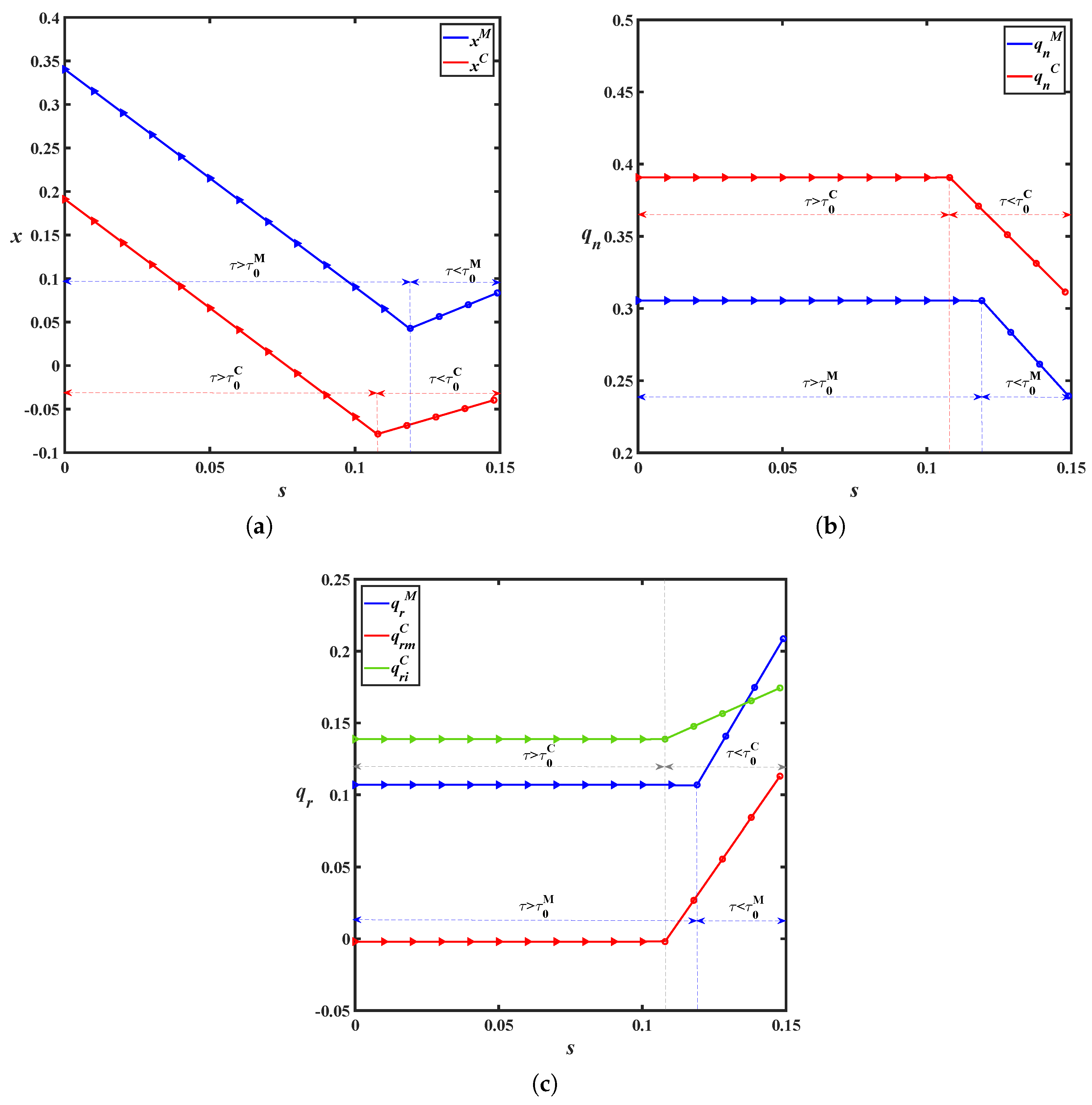
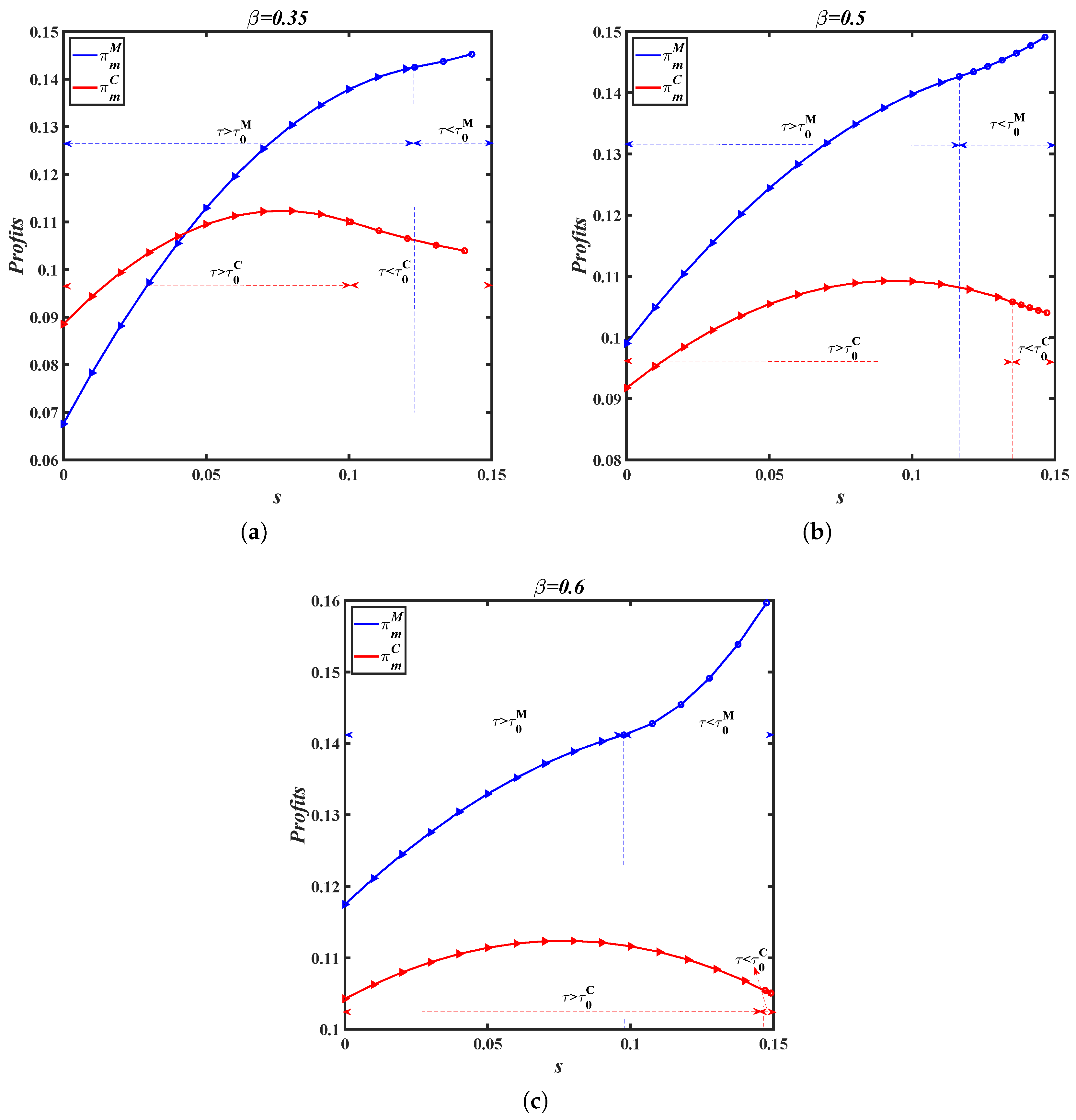
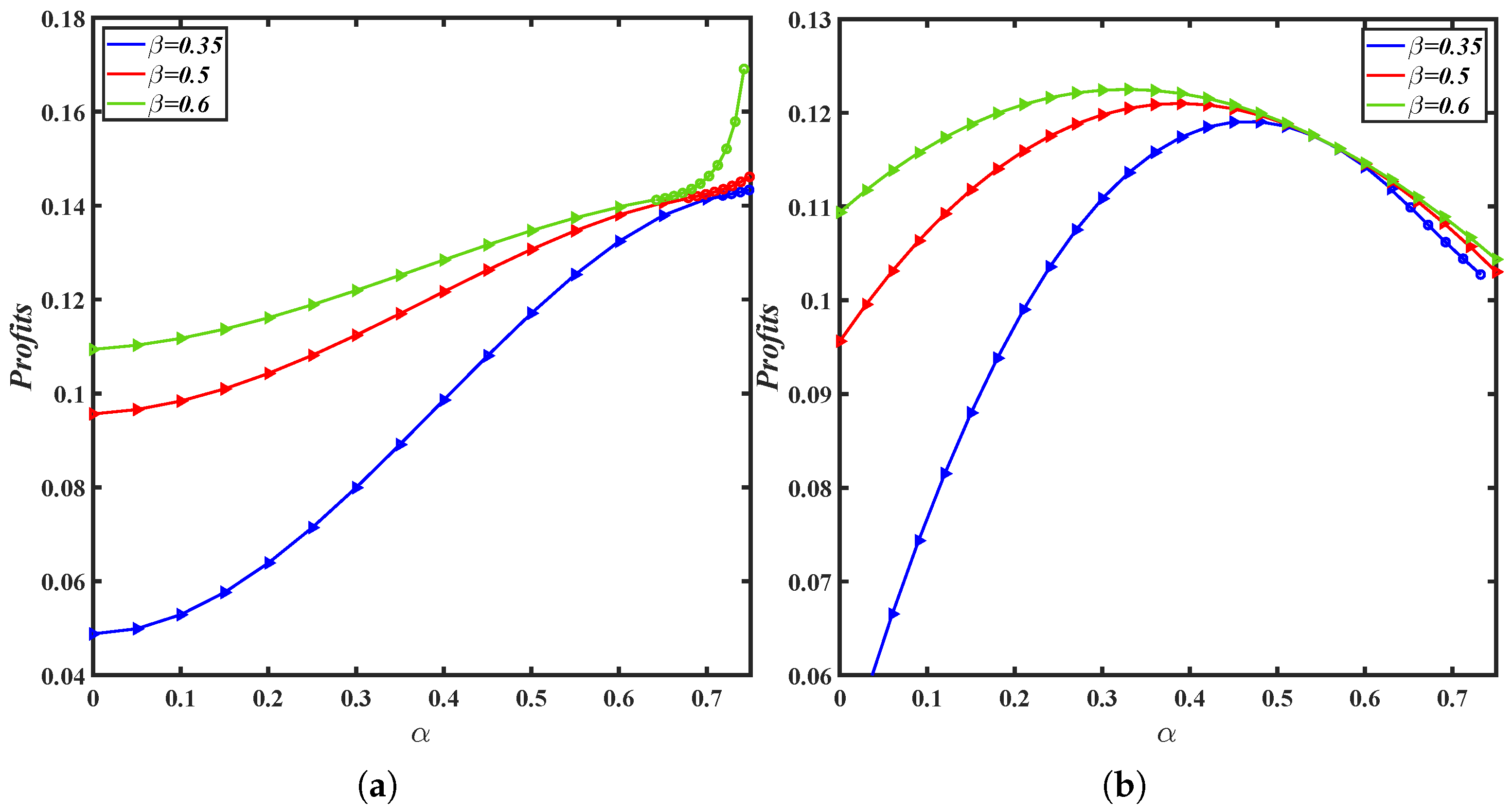
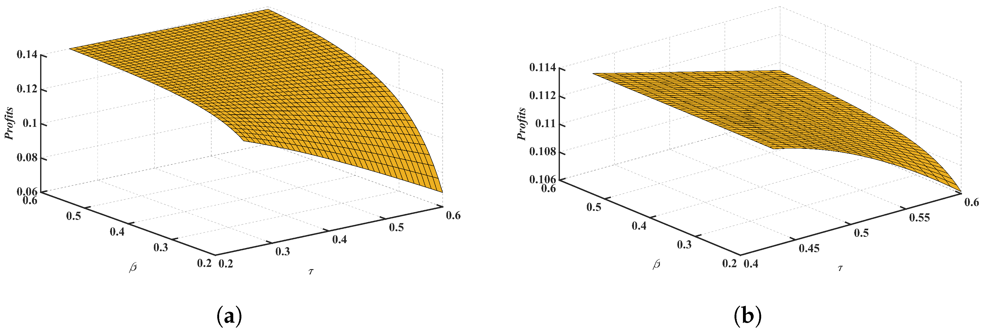
There are many criteria to measure the environmental impact, such as the amount of non-recyclable materials used in the production process, energy consumption, carbon emissions, and so on [19,29]. This paper uses carbon emission as a proxy to investigate the environmental impact. We denote that the carbon emission of a new product is $e_n$, and the carbon emission of a remanufactured product is $e_r$. Therefore, the total environmental impact of the monopolistic remanufacturing scenario is $E{I}^M=e_n{q}_n^M+e_r{q}_r^M$, and the competitive remanufacturing scenario is $E{I}^C=e_n{q}_n^C+e_r(q_{rm}^C+q_{ri}^C)$.

Lemma 4. 

The competition between the OEM and remanufacturer significantly burdens the environmental impact compared with that in a monopolistic scenario, i.e., $E{I}^C>E{I}^M$.

Lemma 4 establishes that the entry of a remanufacturer leads to an increase in carbon emissions, demonstrating that competition in remanufacturing markets inherently exacerbates environmental impacts compared to monopolistic conditions. As evidenced in Lemma 1, the competitive dynamics between the OEM and the remanufacturer prompt an increase in the production of both new and remanufactured products. Given that the cumulative environmental impact is largely determined by the quantity of products manufactured, it simultaneously amplifies resource depletion and emissions through scale effects.

6. Numerical Study

In this section, we present numerical studies to quantify the optimal decisions and profitability as previously discussed, and the impact of take-back regulation on the OEM’s profit will also be presented to validate the reliability and stability of our proposed models.

The growing global market of remanufactured smartphones, which saw a 15% growth in 2021 and is expected to keep expanding (https://www.counterpointresearch.com/insights/global-refurbished-smartphone-market-2021/, acessed on 20 February 2025), highlights the increasing demand and growth potential in the remanufacturing industry for personal electronic products. Leveraging this context, we use mobile phones as a representative case for electronic products, with numerical data derived from case studies and industry reports. Empirical research and case studies have identified a range of consumer preferences for remanufactured products, varying from 0.45 to 0.8 [30]. On platforms like eBay.com, the prices of refurbished iPhone 13 and 13 Pro models with 128 GB can be discounted by 30% to 52%, depending on the quality of the remanufactured products. In light of this, we assign the consumer preference for remanufactured products as $\alpha =65\%$. According to the established models, we calculate the optimal decision variables—the profits in fixed data sets. The specific results are shown in

Table 3. Comparison of optimal solutions under different models.

Data Sets	Solutions
	Model	$\mathit{x}$	${\mathit{q}}_{\mathit{n}}$	${\mathit{q}}_{\mathit{rm}}$	${\mathit{q}}_{\mathit{ri}}$	${\mathit{\pi }}_{\mathit{m}}$	${\mathit{\pi }}_{\mathit{r}}$
Case 1: $c=0.5$, $s=0.1$, $k=1$, $\alpha =0.65$, $\delta =0.75$, $\tau =0.35$, $\beta =0.6$	Model M	0.1791	0.2037	0.0713	/	0.0476	/
	Model C	0.1356	0.2409	0.0631	0.0213	0.0486	0.0002
Case 2: $c=0.25$, $s=0.1$, $k=1$, $\alpha =0.65$, $\delta =0.7$, $\tau =0.35$, $\beta =0.6$	Model M	0.0868	0.3099	0.1085	/	0.1397	/
	Model C	−0.0089	0.3817	0.0187	0.1149	0.1208	0.0055
Case 3: $c=0.5$, $s=0.1$, $k=1$, $\alpha =0.65$, $\delta =0.75$, $\tau =0.1$, $\beta =0.3$	Model M	0.2856	0.2347	0.0235	/	0.0218	/
	Model C	0.2022	0.2705	0.0207	0.0064	0.0396	0.0001
Case 4: $c=0.25$, $s=0.1$, $k=1$, $\alpha =0.65$, $\delta =0.5$, $\tau =0.1$, $\beta =0.3$	Model M	0.0117	0.3521	0.0352	/	0.1408	/
	Model C	−0.0515	0.3792	0.0359	0.0379	0.1330	0.0005

. The selected parameter values ensure positive values of our solutions across all scenarios, providing a robust framework for our analysis. From Table 3, it is evident that the OEM’s DfR investment level in Model M is always higher than that of Model C, which leads to the production quantity of new products in Model M never exceeding that of Model C.

Figure 1 provides a detailed analysis of the relationship between the cost savings of remanufactured s and the optimal decision outcomes in both monopolistic and competitive remanufacturing environments, where we set $c=0.25$, $k=1$, $\alpha =0.65$, $\delta =0.85$, $\tau =0.35$, and $\beta =0.6$. As depicted in Figure 1a, when the take-back regulation is effective, the OEM tends to decrease its DfR investment as s increases. This suggests that under stringent regulatory conditions, the OEM may perceive less need to invest in DfR due to the lower cost savings from remanufacturing. Conversely, when the take-back regulation is ineffective, the OEM increases DfR investment with a rise in s. This indicates that in the absence of effective regulations, the OEM recognizes the profits of investing in DfR to capitalize on the cost savings from remanufacturing. Furthermore, Figure 1c demonstrates that in competitive remanufacturing markets, remanufacturers consistently outperform OEMs in terms of the production quantity of remanufactured products. This can be explained by the remanufacturers’ potential cost advantages in materials and processing, which enable them to price remanufactured products more competitively and consequently secure a larger market share.

We present Figure 2 to discuss the impact of cost savings of remanufactured products s on the OEM’s profit in both monopolistic and competitive remanufacturing environments. As shown in Figure 2, there always is a positive correlation between the OEM’s profit and s in a monopolistic remanufacturing environment. This indicates that as s increases, the OEM’s profits also increase, which is a straightforward economic incentive for investing in remanufacturing capabilities. However, in a competitive remanufacturing environment, the relationship between s and the OEM’s profit is more complex. When the take-back regulation is effective (i.e., $\tau >{\tau }_0^C$), the OEM’s profits increase with s only up to a certain point. Beyond this threshold, a higher s lead to decreased profits for the OEM. This suggests that while cost savings are beneficial, they can also lead to increased competition, which may erode the OEM’s market power and profitability. Conversely, OEM profits consistently decrease with s when the take-back regulation is ineffective (i.e., $\tau <{\tau }_0^C$). This implies that in the absence of effective regulations, the OEM may face a situation where the benefits from remanufacturing are outweighed by competitive pressures, leading to lower profits. This suggests that when take-back regulation is ineffective, OEMs may experience diminishing returns from remanufacturing activities, as competitive pressures could undermine profit margins.

Figure 3 illustrates the impact of consumer preference for remanufactured products $\alpha$ and the remanufacturing cost sensitivity factor to DfR $\beta$ on the OEM’s profit, both in the monopolistic and competitive remanufacturing environments. As shown in Figure 3a, the OEM’s profit is positively correlated with $\alpha$ and $\beta$ in the monopolistic remanufacturing environment. However, Figure 3b demonstrates that the OEM does not always obtain a high profit, as the consumer preference for remanufactured $\alpha$ increases in the competitive remanufacturing environment. This phenomenon occurs because remanufacturers are incentivized to expand production when consumer preference for remanufactured products increases. In competitive markets, such market entry intensifies product cannibalization, ultimately undermining the OEM’s market share and profitability.

Figure 4 presents the implications of $\tau$ on the OEM’s profits when the take-back regulation is effective, by setting $c=0.25$, $s=0.1$, $k=1$, $\alpha =0.65$, and $\delta =0.85$. As shown in Figure 4, a high $\tau$ significantly reduces OEM’s profits. This is because stringent take-back regulations compel OEMs to invest more in remanufacturing activities, which can be costly and may not immediately translate into higher profits. Additionally, according to Figure 4, when the government’s take-back regulation target is effective, an increase in $\beta$ is always beneficial for the OEM to obtain higher profits in both monopolistic and competitive remanufacturing environments. This suggests that the profits of remanufacturing are significantly influenced by the OEM’s ability to manage the remanufacturing process efficiently.

7. Conclusions and Implications

7.1. Conclusions

Governments worldwide have implemented stringent take-back regulations to incentivize e-waste remanufacturing due to growing e-waste accumulation. This stimulates increasingly more e-product original equipment manufacturers (OEMs) to incorporate design for remanufacturing (DfR) during the product design phase. Furthermore, facing competition from independent remanufacturers, OEMs always strategically adjust their DfR strategy to deal with the challenges from internal and external remanufacturing. Currently, the impact of take-back regulations on DfR and remanufacturing decisions remain uncertain in the competitive remanufacturing scenario. In this study, we focus on two different remanufacturing market structures to investigate optimal DfR and remanufacturing decisions under take-back regulations. Specifically, we develop a monopolistic remanufacturing market where an OEM produces both new and remanufactured products as a benchmark model, and the Stackelberg game model involving an OEM and a remanufacturer is established to explore the OEM’s optimal DfR decisions under take-back regulations. Our research yields the following findings:

(1) Mandatory take-back regulations effectively encourage DfR investment and remanufacturing activities only when regulators set a relatively high take-back target. Otherwise, take-back regulations become redundant due to firms already engaging in remanufacturing voluntarily to maximize profits. Unlike in a monopolistic remanufacturing market where the OEM consistently maintains a high DfR investment level, an OEM in a competitive remanufacturing scenario greatly invests in DfR only when remanufacturing cost savings are relatively low. This is because of mandatory take-back regulations. Conversely, if cost savings are high, the OEM tends to reduce DfR investment to increase remanufacturing costs, thereby discouraging third-party remanufacturers from entering the market. In addition, we find that the take-back regulation consistently leads OEMs to increase the DfR investment levels, both in monopolistic and competitive remanufacturing environments. This suggests that stringent take-back regulations are beneficial in promoting product remanufacturability design, thereby enhancing overall remanufacturing activity.

(2) Although the OEM’s optimal DfR investment in competitive markets is consistently lower than in monopolistic settings, the quantity of remanufactured products is invariably higher. This suggests that competition maintains robust market availability for remanufactured products, despite the reduced OEM investment in DfR.

(3) Under ineffective take-back regulations, OEM profits are consistently higher in monopolistic remanufacturing scenarios than in competitive ones. However, when take-back targets become effective, this relationship reverses as follows: the OEM may earn lower profits in monopolistic scenarios than in competitive ones, particularly when remanufacturing cost savings are relatively low. Furthermore, our findings indicate that remanufacturing competition invariably benefits consumer surplus while concurrently increasing the environmental burden.

7.2. Managerial Insights and Implications

In this study, we examine how take-back regulations influence production and DfR decisions in a closed-loop supply chain by analyzing two distinct remanufacturing scenarios. Through the equilibrium solutions derived from our models, we conduct a comprehensive comparative analysis of economic and environmental outcomes. Our findings yield several key managerial implications as follows:

(1) OEMs should strategically determine whether to deter remanufacturers from the remanufacturing market based on both regulatory mandates and remanufactured products’ cost advantages. Specifically, when governments set low take-back targets, monopolistic remanufacturing proves more profitable for OEMs. In such cases, OEMs should implement barriers to third-party remanufacturers’ entry. When the government sets high take-back regulation targets, the decision to prevent third-party remanufacturers from entering the market is contingent upon the cost savings of remanufactured products. When the cost savings from remanufactured products are high, OEMs should allow remanufacturers’ entry to share the regulatory compliance burdens.

(2) The findings reveal that both the cost savings from remanufactured products and the sensitivity of remanufacturing costs to DfR significantly influence the OEM’s DfR investment levels and profitability. Therefore, managers should systematically evaluate and identify profitable DfR opportunities to maximize returns on DfR investments.

(3) For policymakers, take-back regulations consistently motivate OEMs to invest in DfR, thereby enhancing remanufacturing activities and generating environmental benefits. Therefore, it is advisable for the government to proactively implement take-back regulations. This is particularly crucial in the markets where third-party remanufacturers actively participate in remanufacturing, as take-back regulations can counterbalance OEMs’ attempts to block remanufacturers’ entry into the market.

Several limitations of this study should be acknowledged. First, our proposed models primarily assume a deterministic environment where the quality of collected products and market demand are certain. However, in reality, the market is often characterized by various uncertainties. It would be more valuable to construct a model that incorporates these uncertainties to better assess the impact of take-back regulations on OEMs’ decisions within a CLSC. Second, to simplify the model, we have ignored the relationship between collectors and the associated collection costs. In practice, different collectors may incur varying costs when collecting used products. Including these relationships in future models could reveal more insightful and meaningful results, and this is an area that warrants further exploration. Finally, in this study, we mainly focus on the implications of take-back regulations, while other significant environmental legislation such as carbon tax and carbon cap-and-trade are also widely enacted by governments. Future research could benefit from examining the combined effects of these various carbon policies along with take-back regulations on remanufacturing practices.

References

1. Psarommatis, F.; May, G. A Cost–Benefit Model for Sustainable Product Reuse and Repurposing in Circular Remanufacturing. Sustainability 2025, 17, 245. [Google Scholar] [CrossRef]
2. Tabassum, M.; Nemani, V.; Hu, C.; Kremer, G.E. A novel design optimization framework to sustain remanufacturability. J. Clean. Prod. 2024, 479, 143935. [Google Scholar] [CrossRef]
3. Hong, Z.; Zhang, Y.; Yu, Y.; Chu, C. Dynamic pricing for remanufacturing within socially environmental incentives. Int. J. Prod. Res. 2020, 58, 3976–3997. [Google Scholar] [CrossRef]
4. Yang, D.; Yang, Q.; Zhang, L. Operational Decisions on Remanufacturing under the Product Innovation Race. Sustainability 2023, 15, 4920. [Google Scholar] [CrossRef]
5. Huang, Q.; Hou, J.; Shen, H. Remanufacturing and pricing strategies under modular architecture. Comput. Ind. Eng. 2024, 188, 109863. [Google Scholar] [CrossRef]
6. Zhang, L.; Li, K.; Chu, C.; Liu, J. Investment and remanufacturing strategies considering the application of intelligent manufacturing in hybrid manufacturing–remanufacturing systems. Expert Syst. Appl. 2024, 257, 124991. [Google Scholar] [CrossRef]
7. Long, X.; Ge, J.; Shu, T.; Liu, Y. Analysis for recycling and remanufacturing strategies in a supply chain considering consumers’ heterogeneous WTP. Resour. Conserv. Recycl. 2019, 148, 80–90. [Google Scholar] [CrossRef]
8. Fang, C.; You, Z.; Yang, Y.; Chen, D.; Mukhopadhyay, S. Is third-party remanufacturing necessarily harmful to the original equipment manufacturer? Ann. Oper. Res. 2020, 291, 317–338. [Google Scholar] [CrossRef]
9. Tang, S.; Wang, W.; Zhou, G. Remanufacturing in a competitive market: A closed-loop supply chain in a Stackelberg game framework. Expert Syst. Appl. 2020, 161, 113655. [Google Scholar] [CrossRef]
10. Wang, Y.; Wang, Z.; Gong, Y.; Li, B.; Cheng, Y. The implications of the carbon tax on the vehicle remanufacturing industry in the complex competitive environment. Manag. Decis. Econ. 2023, 44, 2697–2712. [Google Scholar] [CrossRef]
11. Tabassum, M.; De Brabanter, K.; Kremer, G.E. Surrogate-assisted optimization under uncertainty for design for remanufacturing considering material price volatility. Sustain. Mater. Technol. 2024, 42, e01163. [Google Scholar] [CrossRef]
12. Shi, T.; Gu, W.; Chhajed, D.; Petruzzi, N.C. Effects of Remanufacturable Product Design on Market Segmentation and the Environment. Decis. Sci. 2016, 47, 298–332. [Google Scholar] [CrossRef]
13. Liu, Z.; Li, K.W.; Li, B.Y.; Huang, J.; Tang, J. Impact of product-design strategies on the operations of a closed-loop supply chain. Transp. Res. Part E Logist. Transp. Rev. 2019, 124, 75–91. [Google Scholar] [CrossRef]
14. Shahbazi, S.; Johansen, K.; Sundin, E. Product Design for Automated Remanufacturing—A Case Study of Electric and Electronic Equipment in Sweden. Sustainability 2021, 13, 9039. [Google Scholar] [CrossRef]
15. Hu, Y.; Chen, L.; Chi, Y.; Song, B. Manufacturer encroachment on a closed-loop supply chain with design for remanufacturing. Manag. Decis. Econ. 2022, 43, 1941–1959. [Google Scholar] [CrossRef]
16. Zhou, Y.; Hou, M.; Wong, K.H. The Optimal Remanufacturing Strategy of the Closed-Loop Supply Chain Network under Government Regulation and the Manufacturer’s Design for the Environment. Sustainability 2023, 15, 7342. [Google Scholar] [CrossRef]
17. Esenduran, G.; Kemahlıoğlu-Ziya, E.; Swaminathan, J.M. Impact of take-back regulation on the remanufacturing industry. Prod. Oper. Manag. 2017, 26, 924–944. [Google Scholar] [CrossRef]
18. Pazoki, M.; Samarghandi, H. Take-back regulation: Remanufacturing or eco-design? Int. J. Prod. Econ. 2020, 227, 107674. [Google Scholar] [CrossRef]
19. Kushwaha, S.; Chan, F.T.; Chakraborty, K.; Pratap, S. Collection and remanufacturing channels selection under a product take-back regulation with remanufacturing target. Int. J. Prod. Res. 2022, 60, 7384–7410. [Google Scholar] [CrossRef]
20. Liu, H.; Ye, L.; Sun, J. Automotive parts remanufacturing models: Consequences for ELV take-back under government regulations. J. Clean. Prod. 2023, 416, 137760. [Google Scholar] [CrossRef]
21. Cao, J.; Wu, S.; Kumar, S. Recovering and remanufacturing to fulfill EPR regulation in the presence of secondary market. Int. J. Prod. Econ. 2023, 263, 108933. [Google Scholar] [CrossRef]
22. He, J.; Yan, W.; Li, Y.; Lu, D. Recycling and/or reusing: When product innovation meets the recast of WEEE direct. Int. J. Prod. Res. 2024, 62, 7018–7029. [Google Scholar] [CrossRef]
23. Wei, F.; Huang, Q. Operational decisions for remanufactured products in a sustainable supply chain. Ann. Oper. Res. 2024. [Google Scholar] [CrossRef]
24. Zhou, Q.; Meng, C.; Sheu, J.B.; Yuen, K.F. Impact of Market Competition on Remanufacturing Investment. IEEE Trans. Eng. Manag. 2023, 71, 6995–7014. [Google Scholar] [CrossRef]
25. Reimann, M.; Xiong, Y.; Zhou, Y. Managing a closed-loop supply chain with process innovation for remanufacturing. Eur. J. Oper. Res. 2019, 276, 510–518. [Google Scholar] [CrossRef]
26. Zhou, J.; Xu, H.; Deng, Q.; Ma, Y.; Luo, Q. Two-stage optimal acquisition and remanufacturing decisions with demand and quality information updating. Transp. Res. Part E Logist. Transp. Rev. 2024, 192, 103823. [Google Scholar] [CrossRef]
27. Panagiotidou, S. Joint optimization of manufacturing/remanufacturing lot sizes under imperfect information on returns quality. Eur. J. Oper. Res. 2017, 258, 537–551. [Google Scholar] [CrossRef]
28. Liao, H.; Zhang, Q.; Li, L. Optimal procurement strategy for multi-echelon remanufacturing systems under quality uncertainty. Transp. Res. Part E Logist. Transp. Rev. 2023, 170, 103023. [Google Scholar] [CrossRef]
29. Zhu, C.; Xi, X.; Goh, M. Differential game analysis of joint emission reduction decisions under mixed carbon policies and CEA. J. Environ. Manag. 2024, 358, 120913. [Google Scholar] [CrossRef]
30. Abbey, J.D.; Kleber, R.; Souza, G.C.; Voigt, G. Remanufacturing and consumers’ risky choices: Behavioral modeling and the role of ambiguity aversion. J. Oper. Manag. 2019, 65, 4–21. [Google Scholar] [CrossRef]
Figure 1. Optimal solutions in monopolistic and competitive scenarios. (a) DfR investment level. (b) Production quantity for new products. (c) Production quantity for remanufactured products.
Sustainability 17 03593 g001
Figure 2. OEM profits in monopolistic and competitive scenarios. (a) Low cost sensitivity to DfR. (b) Medium cost sensitivity to DfR. (c) High cost sensitivity to DfR.
Sustainability 17 03593 g002
Figure 3. Effect of α on the OEM’s profits. (a) Monopolistic scenario. (b) Competitive scenario.
Sustainability 17 03593 g003
Figure 4. Effect of τ and β on the OEM’s profits. (a) Monopolistic scenario. (b) Competitive scenario.
Sustainability 17 03593 g004