Assessment of Water Quality and Ecological Integrity in an Ecuadorian Andean Watershed

Abstract

This study assessed the water quality and ecological integrity of the Columbe River micro-watershed in the Ecuadorian Andes through a multidimensional approach incorporating biotic, physicochemical, and structural indices. Indices such as the Andean Biotic Index (ABI), Biological Monitoring Working Party index adapted for Colombian conditions (BMWP-Col), Fluvial Habitat Index (IHF), Riparian Quality Index adapted for Andean conditions (QBR-And), and Water Quality Index (WQI) characterized environmental quality gradients and evaluated the impact of human activities across 11 monitoring sites. Hierarchical cluster analysis classified sampling sites into three groups: less polluted (LP), moderately polluted (MP), and highly polluted (HP). HP sites showed elevated levels of biochemical oxygen demand (BOD₅), chemical oxygen demand (COD), electrical conductivity (EC), and turbidity, alongside low biotic and structural scores, indicating advanced ecological degradation. Conversely, LP sites demonstrated greater ecological integrity, despite elevated BOD₅ and COD levels across the watershed, suggesting widespread diffuse contamination. The findings identify anthropogenic activities such as livestock, agriculture, and domestic discharges as major pressures on water quality and macroinvertebrate biodiversity. Significant correlations between physicochemical parameters—including BOD₅ and EC—and declining biotic indices underscore the link between chemical water degradation and ecological fragmentation. In this context, this study highlights the critical need for comprehensive management and restoration strategies to combat pollution, safeguard relatively pristine areas, and rehabilitate the ecological integrity and connectivity of high-altitude Andean aquatic ecosystems under anthropogenic pressure.

1. Introduction

The ecological integrity of fluvial ecosystems is essential for sustaining biodiversity, maintaining hydrological stability, and supporting water-dependent socio-economic activities. In mountainous regions such as the tropical Andes, these systems are particularly important due to their elevation-driven hydrological dynamics and ecological richness [1,2]. High-Andean micro-watersheds, in particular, support regional water security, but are increasingly threatened by expanding agriculture, livestock grazing, deforestation, urban encroachment, and infrastructure development [2,3].

The Andean landscape forms a complex mosaic shaped by both natural variability and anthropogenic pressure. A steep topography and sharp altitudinal gradients produce sensitive hydrological systems, where páramos and riparian corridors help buffer disturbances and maintain ecological balance [1,4]. However, the upward shift of land-use activities—often replacing native vegetation with pastures or croplands—contributes to erosion, nutrient loading, and habitat fragmentation [5,6]. In parallel, the limited reach of wastewater treatment in rural areas results in untreated discharges, intensifying fecal contamination and organic pollution [7,8]. These transformations reduce ecosystem functionality, which becomes evident in degraded habitat structure and altered macroinvertebrate communities [2,3].

Ecological assessments based solely on physicochemical parameters offer only momentary snapshots of water conditions and often fail to capture cumulative or chronic stressors. For this reason, biotic indices like the Andean Biotic Index (ABI) and the Biological Monitoring Working Party index adapted to Colombia (BMWP-Col) are widely used [9,10,11,12]. These tools evaluate macroinvertebrate community responses to pollution and help classify ecosystem health based on species sensitivity to environmental stress [13,14]. Structural indices such as the Fluvial Habitat Index (IHF) and the Riparian Forest Quality Index adapted for Andean conditions (QBR-And) assess physical heterogeneity and riparian condition, factors that are central to ecological resilience [12,15,16]. Additionally, the Water Quality Index (WQI) integrates multiple physicochemical parameters to provide an overall picture of water pollution, making it useful for characterizing pressure gradients in fluvial systems [7,17].

Although these indices have proven useful in Andean contexts, many studies apply them in isolation [2,7,10,11], which limits the understanding of how physical, chemical, and biological factors interact. In several cases, tolerance values are based on generalized regional datasets and may not reflect the specific environmental dynamics of local watersheds. Moreover, spatial methods that could reveal pollution gradients or priority areas for conservation remain underused in routine biomonitoring.

A growing number of studies across the Andean region have begun to document how environmental pressures are reflected in ecological indicators. For example, Hampel et al. reported a sharp decline in riparian vegetation and fluvial habitat scores (QBR: from 82.4 to 10; IHF: from 60.3 to 39) in the Paute River Basin (Ecuador) due to cattle grazing and riparian degradation [2]. Similarly, Vargas-Tierras et al. found a decrease in BMWP-Col scores (from 72 to 47) in the Yanaquincha River linked to wastewater discharges [11]. Studies in Colombia, Peru, and Costa Rica have described comparable degradation patterns caused by agricultural runoff, infrastructure development, and vegetation loss [12,18,19]. However, many of these works emphasize either biological or chemical metrics, rather than using integrated frameworks.

This study addresses those methodological limitations by applying a multidimensional approach to assess ecological integrity in the Columbe River micro-watershed (Ecuadorian Andes). It combines biotic (ABI, BMWP-Col), structural (IHF, QBR-And), and physicochemical (WQI) indices to produce a comprehensive evaluation of ecosystem health. In addition, hierarchical clustering is used to classify sampling points spatially, uncovering patterns of degradation and identifying zones with conservation or restoration potential. This spatial classification not only supports the ecological diagnosis of the watershed but also contributes to sustainable planning by identifying priority zones for targeted intervention. By distinguishing areas requiring conservation from those demanding restoration, this study provides actionable input for integrated watershed management. This aligns with sustainability goals by promoting land-use decisions that maintain ecosystem services, reduce downstream contamination, and foster long-term resilience in socio-environmentally vulnerable Andean regions. The application of this spatially explicit approach also supports the local implementation of sustainability frameworks, such as payment for ecosystem services (PES) and nature-based solutions, which have proven effective in reconciling environmental conservation with rural development objectives [20,21].

The novelty of this research lies in the simultaneous application of five complementary indices within a single Andean watershed, offering a more nuanced and accurate diagnosis of ecological conditions. Unlike earlier studies that often rely on a limited set of indicators, this approach enables site-specific interpretation and strengthens the operational basis for watershed planning and intervention in data-scarce, environmentally pressured regions.

2. Materials and Methods

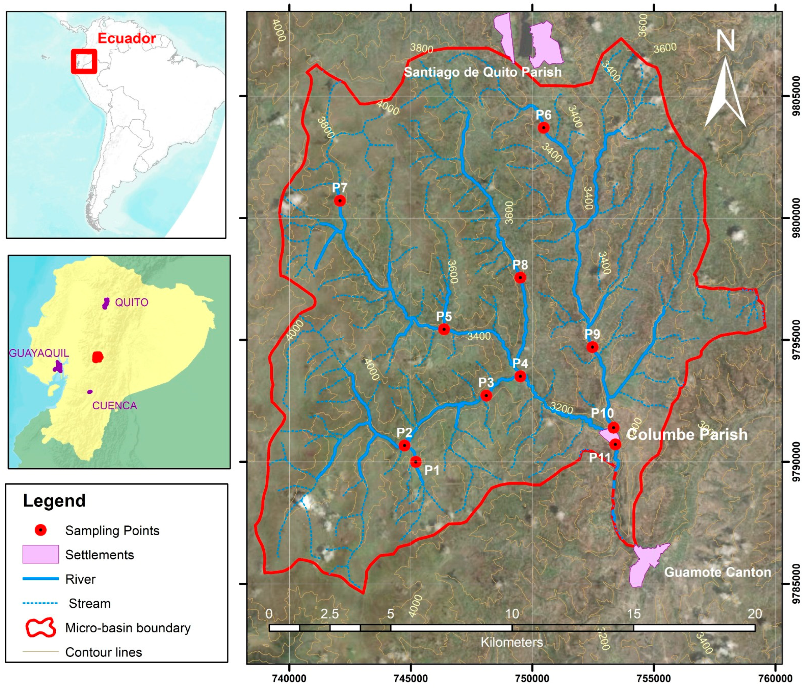
2.1. Study Area and Monitoring Samples

The present study was conducted in the Columbe River micro-watershed, which covers an area of 309.13 km² and is located in the Columbe parish, Colta canton, Chimborazo province. It features a characteristic Ecuadorian Andean climate, with an average annual temperature of 11 °C [22]. Its altitudinal range spans from 3080 to 4320 m above sea level, contributing to remarkable microclimatic and ecological diversity [23]. Annual precipitation varies significantly, with minimum values of 500 mm, maximum values of 1250 mm, and an average of 780 mm [23]. The soil taxonomy in the Columbe parish is classified into Inceptisols (44%), Mollisols (30%), Entisols (25%), and Histosols (1%), reflecting significant edaphic heterogeneity [22]. Regarding land use and cover, agricultural areas dominate, occupying 62.23% of the territory, followed by shrub and herbaceous vegetation (34.73%), desertified areas (2.82%), anthropogenic zones (0.17%), and water bodies (0.04%) [22,23]. The ecosystems include Evergreen Montane Shrubland of the Northern Andes, Evergreen Shrubland and Grassland of the Páramo, Páramo Grassland, Subnival Evergreen Grassland and Shrubland of the Páramo, and Intervention Zones, reflecting the climatic and altitudinal conditions of the micro-watershed [22,23]. The micro-watershed consists of páramo-origin tributaries, including the Guashi River, Sasapud River, Guahuijón River, Llinllín Creek, Pulucate Creek, Llinllín River, and several secondary drainages [24].

Sampling locations were strategically selected based on environmental representativeness. Priority was given to sites with direct effluent discharges, areas affected by livestock and agricultural activities, and zones near human settlements to assess the impact of anthropogenic activities. Additionally, locations in areas free from human settlements were included to establish reference points for comparing impacted and non-impacted environments. To ensure a representative sample, 11 monitoring points were selected within the micro-watershed, as shown in Figure 1.

Point 1 was chosen in an area with no visible human disturbances, representing minimally impacted headwaters. Points 2-to-11 were distributed along the watershed, covering zones with varying degrees of agricultural use, livestock presence, and proximity to human settlements.

Three monitoring sessions were conducted at each point to measure physicochemical parameters, ensuring temporal consistency and data reliability. Macroinvertebrate sampling and the corresponding components used to calculate ecological indices were assessed through a single campaign. All field activities were carried out between September 2023 and March 2024 under comparable climatic conditions, ensuring uniform environmental settings throughout the monitoring period.

Five indices were applied to assess water quality and ecological integrity in the Columbe River micro-watershed, each addressing different ecological dimensions: aquatic biodiversity (ABI, BMWP-Col), habitat structure (IHF, QBR-And), and physicochemical status (WQI-TULSMA).

The Andean Biotic Index (ABI) and the Biological Monitoring Working Party index adapted for Colombia (BMWP-Col) were chosen over other alternatives, such as the Neotropical Lowland Stream Multimetric Index (NLSMI) or multimetric indices like the Index of Biotic Integrity (IBI) and the Multimetric Macroinvertebrate Index (MMI). These alternatives typically require genus- or species-level taxonomic data, which can be difficult to obtain in regions with a limited taxonomic infrastructure [25,26,27]. Moreover, indices like the IBI and MMI may be less suitable for high-altitude environments, where the taxa composition and environmental dynamics differ significantly from lowland systems [26,27]. The NLSMI, for example, was found to be less appropriate for the Guayas River Basin compared to the BMWP-Col due to its complexity and the need for a wider range of metrics [25]. In contrast, the ABI and BMWP-Col rely on family level identification and assign explicit sensitivity scores, making them more practical and interpretable for applied monitoring in high-Andean watersheds.

For structural evaluation, the Fluvial Habitat Index (IHF) and the Riparian Vegetation Quality Index adapted for Andean conditions (QBR-And) were specifically chosen over global tools like the River Habitat Survey (RHS) or Rapid Bioassessment Protocols (RBPs). These latter tools were primarily developed for lowland temperate systems and are not as effective in high-altitude Andean environments due to differences in geomorphological and ecological characteristics [28]. The RHS and RBPs are tailored to regions with more uniform topography and less pronounced altitude-driven environmental gradients, making them less suitable for the heterogeneous and ecologically diverse nature of Andean rivers [28,29]. In contrast, although the IHF was not originally designed for Andean systems, it has proven effective in capturing habitat features such as substrate diversity and flow variability in mountain streams, making it suitable for use in high-Andean environments when adapted along with the QBR-And [2,12,19].

The Water Quality Index (WQI) was chosen due to its alignment with national environmental standards and its incorporation of region-specific parameters, making it a more contextually relevant tool for assessing water quality in high-Andean ecosystems. In contrast to general models such as the NSF-WQI or CCME-WQI, which may not fully capture local environmental variations, the WQI provides a tailored evaluation that reflects the unique ecological and regulatory conditions of the region. This approach is consistent with the findings of studies like Lukhabi et al. (2023) and Uddin et al. (2018), which emphasized the importance of using locally adapted indices to enhance the accuracy of water quality assessments, particularly in areas with distinct ecological characteristics [30,31].

2.2. Water Quality Parameters

Water samples were collected following the Standard Methods for the Examination of Water and Wastewater (APHA, 2017). In situ physicochemical parameters—including temperature, pH, electrical conductivity (EC), dissolved oxygen (DO), total dissolved solids (TDS), and salinity—were measured using a Hanna Instruments HI98194 multiparameter meter (Hanna Instruments, Woonsocket, RI, USA). This device features GLP (Good Laboratory Practice) functions for calibration traceability and complies with IP67 standards, ensuring durability under harsh field conditions [32].

For laboratory analyses, water samples were collected in appropriate containers and preserved following standard protocols. Chemical parameters included sulfates (SO₄²⁻), analyzed by turbidimetry using a Hach TL2300 benchtop turbidimeter (Hach Company, Loveland, CO, USA) (APHA 4500-SO₄²⁻ E); phosphates (PO₄³⁻), nitrates (NO₃⁻), nitrites (NO₂⁻), and fluorides (F⁻) were quantified using a Hach DR6000 UV–Vis spectrophotometer (Hach Company, Loveland, CO, USA), applying the ammonium molybdate method (APHA 4500-P E), UV spectrophotometry (APHA 4500-NO₃⁻ B), Griess reagent method (APHA 4500-NO₂⁻ B), and SPADNS reagent method (APHA 4500-F⁻ D), respectively.

Additionally, organic pollution indicators were assessed, including chemical oxygen demand (COD), determined by the closed reflux method with potassium dichromate using a Hach DRB200 digestion block (Hach Company, Loveland, CO, USA), followed by spectrophotometric reading with a Hach DR6000 UV–Vis spectrophotometer (Hach Company, Loveland, CO, USA) (APHA 5220 D), and biochemical oxygen demand over five days (BOD₅), measured by controlled incubation in a Memmert IN30 incubator (Memmert GmbH, Schwabach, Germany) (APHA 5210 B). For microbiological parameters, fecal coliforms were quantified using a Millipore manifold filtration system, followed by incubation on selective medium (m-FC agar) using the Memmert IN30 incubator (Memmert GmbH, Schwabach, Germany) (APHA 9222 D).

2.3. Hydrological Characterization

Flow data for each sampling point were obtained from Valladares-Pogo (2024) [33], using the velocity–area method recommended by the ICC [34]. Measurements involved dividing the river cross-section into segments, calculating area based on depth and width, and recording water velocity using a Global Water FP111 flow meter (Global Water Instrumentation, Gold River, CA, USA). The average velocity was estimated using the 0.2–0.8 depth method, and a correction factor was applied based on stream characteristics, following the recommendations outlined in the Hydrometry Manual developed by national authorities [35]. These measurements were taken during the same season as the water quality assessments conducted for this study. The resulting values are shown in

Table 1. Flow values at each sampling point. Reprinted with permission from ref. [33]. Copyright 2024 Escuela Superior Politécnica de Chimborazo.

Monitoring Point	Flow (m3/s)
P1	0.017
P2	0.623
P3	0.845
P4	0.379
P5	0.685
P6	0.419
P7	0.065
P8	0.156
P9	0.217
P10	0.166
P11	0.856

.

2.4. Sampling of Macroinvertebrates

Benthic macroinvertebrates were collected using a D-frame net and the kick sampling method, a standardized procedure widely applied in bioassessment studies [36,37]. The net, featuring a 30 cm-wide steel frame, a “D”-shaped opening, and a 500-micrometer mesh, is designed to capture macroinvertebrates of various sizes while retaining fine particles. It was positioned on the riverbed with the opening facing downstream. The substrate in front of the net was disturbed by controlled foot kicks, dislodging organisms attached to sediments, rocks, and organic matter. Sampling at each site was conducted for a standardized duration of 3 min, ensuring thorough coverage of the main substrate types present (gravel, sand, rocks, and aquatic vegetation).

Collected samples were transferred to pre-labeled containers with 70% alcohol for preservation and transport to the laboratory. Macroinvertebrates were identified under a Leica EZ4 stereoscope following the simplified protocol for evaluating the environmental quality of Andean rivers (CERA-S) [16].

2.5. Determination of Biotic and Abiotic Indices

2.5.1. Aquatic Biotic Biodiversity

The ABI is based on the original BMWP and adapted for rivers located 2000 m above sea level [13]. It considers the reduced number and distribution of macroinvertebrate families in high-elevation ecosystems, where altitude limits both diversity and sensitivity to disturbance [9,13]. Families are assigned tolerance scores from 1 (high tolerance) to 10 (high sensitivity), and the index value is calculated as the sum of scores for all families present at each site. Sites are classified into five ecological quality levels: >96 (very good), 59–96 (good), 35–58 (moderate), 14–34 (poor), and <14 (very poor) [9].

The BMWP-Col is an adaptation of the original BMWP to Colombian high-mountain rivers and is widely used in Andean ecosystems [9,14]. Its development was based on an exhaustive review of water quality studies using macroinvertebrates, allowing for contextualization and adaptation to the specific taxonomic and environmental conditions of the Andean region [14]. The index considers only the presence or absence of macroinvertebrate families, each assigned a tolerance score ranging from 1 (tolerant) to 10 (sensitive). The final score for each site corresponds to the sum of the values of all families present. The classification categories are as follows: >150 (very-clean-to-clean water), 61–100 (slightly polluted), 36–60 (moderately polluted), 16–35 (heavily polluted), and <15 (very heavily polluted) [14].

While both indices are based on macroinvertebrate sensitivity to pollution, the ABI is specifically tailored to high-altitude Andean rivers with reduced faunal richness, whereas the BMWP-Col encompasses a broader range of families, representative of the ecological variability across Andean mountain systems.

2.5.2. Fluvial Habitat Structure

The Fluvial Habitat Index (IHF) evaluates the physical quality of riverine environments based on seven specific components: substrate inclusion, frequency of riffles, substrate composition, flow velocity and depth regimes, riverbed shading, structural heterogeneity, and aquatic vegetation cover [15]. Each component is scored independently, contributing to a maximum possible score of 100. Higher values indicate more diverse and ecologically functional river habitats. The ecological condition is categorized as follows: ≥90 (very high diversity), 71–80 (high), 50–70 (moderate), 31–49 (low), and 0–30 (very low) [15].

Table 2. Description of the components included in the Fluvial Habitat Index (IHF). Adapted from Pardo et al. (2002) [15].

IHF Component	Definition	Ecological Relevance	Maximum Score
Substrate inclusion and limitation	Refers to the presence of compacted sand between coarse substrates.	Less embeddedness supports more habitat availability for macroinvertebrates.	10
Frequency of riffles	Assesses the number of riffles in the reach.	Riffles create habitat diversity and enhance oxygenation.	10
Substrate composition	Evaluates the diversity of substrate types present.	Diverse substrates support varied benthic communities.	20
Speed/depth regimes	Assesses the presence of combinations of flow velocity and depth.	A wider range of flow conditions promotes species richness.	10
Shade on the riverbed	Estimates shading from riparian vegetation.	Shading regulates temperature and supports aquatic life.	10
Riverbed heterogeneity	Considers the presence of woody debris, roots, and natural barriers.	Structural complexity improves refuge and habitat quality.	10
Aquatic vegetation cover	Quantifies aquatic vegetation types.	Vegetation supports food webs and habitats for colonization.	30

summarizes the components, scoring rationale, and ecological interpretation.

The QBR-And, proposed by Acosta et al. (2009) [16], is an adaptation of the Riparian Vegetation Quality Index (QBR) developed by Munné et al. (2003) [38]. It is specifically designed to evaluate the unique characteristics of Andean vegetation formations and associated riparian typologies, such as rocky banks, páramos, and punas. The QBR-And focuses on four components: vegetation cover, structural complexity, vegetation composition (native vs. introduced), and the degree of channel naturalness. Each category is scored on a tiered scale (0, 5, 10, or 25), and adjustment factors (ranging from −10 to +10) may be applied according to the criteria in the CERA protocol, depending on aspects such as forest connectivity or distribution pattern. The total score ranges from 0 to 100, with quality classifications defined as ≥96 (very good), 76–95 (slightly altered), 51–75 (moderately altered), 26–50 (strongly altered), and ≤25 (extremely degraded) [16].

Table 3. Description of the components included in the adapted Riparian Vegetation Quality Index for the Andes (QBR-And). Adapted from Acosta et al. (2009) [16].

QBR-and Component	Definition	Ecological Relevance	Maximum Score
Riparian zone coverage	Evaluates vegetation cover on riverbanks.	Greater cover implies better erosion control and habitat quality.	25
Vegetation structure	Assesses vertical stratification and species diversity.	Structural complexity is associated with mature riparian systems.	25
Riparian vegetation quality	Evaluates the presence of native vs. exotic species and anthropogenic impact.	Native vegetation and minimal disturbance increase ecological value.	25
Degree of naturalness	Considers the extent of channel modification.	Natural channels offer better habitat continuity and ecological function.	25

outlines the component definitions and their ecological significance.

2.5.3. Physicochemical and Microbiological Water Quality

Anthropogenic stress was assessed through the calculation of a Water Quality Index (WQI), integrating physicochemical and microbiological parameters, with reference to the maximum permissible limits to preserve aquatic life specified in Annex 1 of Book VI of the Unified Text of Secondary Legislation of the Ministry of the Environment of Ecuador (TULSMA, for its acronym in Spanish). The parameters considered for the WQI calculation in this study are those that have established limits in the TULSMA regulations, including true color, biochemical oxygen demand (BOD₅), chemical oxygen demand, fluorides, nitrates, nitrites, dissolved oxygen, pH, total dissolved solids, sulfates, turbidity, and fecal coliforms.

The WQI calculation involved three steps [17]. The first step determined weights for the analyzed parameters, ranging from 1 to 5. These weights reflect the relative importance of each parameter in maintaining water quality for aquatic life. Using these weights, the relative weight of each parameter was computed with Equation (1):

$$W_i={\displaystyle \frac{w_i}{\sum _{i=1}^n{w}_i}}$$

(1)

where W_i is the relative weight, w_i is the weight of each parameter, and n is the total number of parameters.

The second step involved determining the quality rating for each parameter by dividing its concentration in the water sample by the standard established in the Ecuadorian TULSMA regulations and multiplying the result by 100 (Equation (2)).

$$qi={\displaystyle \frac{Ci}{Si}}\times 100$$

(2)

where qi represents the quality rating, Ci is the parameter concentration, and Si is the standard value from TULSMA.

Finally, the WQI evaluation determined a sub-index for each parameter and then summed all sub-indices for each sample (Equations (3) and (4)):

$$SIi=Wi\times qi$$

(3)

$$WQI=\sum _{i=1}^{n}SIi$$

(4)

where SIi is the sub-index for the i-th parameter.

Based on the final WQI value, water quality is classified into five categories: 0–25 (very clean), 26–50 (clean), 51–75 (moderately polluted), 76–100 (polluted), and >100 (dirty) [17].

A unified scale was used to compare methods for parametrizing ecological integrity and water quality in the Andean micro-watershed. The threshold values for the ranges of the ABI, BMWP-Col, IHF, QBR-And, and WQI indices were reviewed, resulting in the identification of five classes, as shown in

Table 4. Classifications and scores of used indices.

Classification Index	Excellent	Good	Fair	Poor	Very Poor
Biotic indices
ABI	>96	59–96	35–58	14–34	<14
BMWP-Col	≥150	61–100	36–60	16–35	<15
Abiotic indices
IHF	≥90	71–80	50–70	31–49	0–30
QBR-And	≥96	76–95	51–75	26–50	≤25
Physicochemical index
WQI	≤25	26–50	51–75	76–100	>100

.

2.6. Data Processing

The drainage basin of the Columbe River was delineated using a 10 m-resolution Digital Elevation Model (DEM) and processed in QGIS 3.16. Hydrological tools, including fill sinks, flow direction, and flow accumulation, were applied to generate the watershed boundary and stream network. This geospatial delineation was verified against official topographic maps provided by the Military Geographic Institute of Ecuador (IGM, for its acronym in Spanish) [39], ensuring consistency with national cartographic standards.

The Pearson correlation coefficient was calculated to identify significant relationships (p < 0.01) between the water quality parameters and the ecological indices.

To explore spatial patterns, a hierarchical agglomerative cluster analysis (CA) was performed using the Ward linkage method and Euclidean distance applied to standardized values (Z-scores) of 22 variables: 17 physicochemical parameters and 5 ecological indices. Standardization was necessary to homogenize variable scales and ensure comparability across different units of measurement. This clustering method was selected due to its demonstrated ability to produce compact and interpretable groupings, which is particularly advantageous in environmental assessments [40,41]. To validate the robustness of the clustering solution, a sensitivity analysis was carried out by comparing results across alternative linkage methods (single, complete, average) and distance metrics (cityblock and correlation). Furthermore, the agglomeration coefficient schedule was reviewed to determine the optimal number of clusters. A marked increase in the coefficient value between successive fusion stages was used as the criterion for selecting the cut-off point, thereby avoiding reliance solely on visual inspection of the dendrogram.

To assess whether the clusters significantly differed in terms of environmental conditions, a one-way ANOVA was applied to each of the 22 variables. When statistically significant differences were found (p < 0.05), Tukey’s Honestly Significant Difference (HSD) post hoc test was used to determine which specific groups differed from each other.

All statistical analyses were conducted using RStudio (version 2023.12.0).

3. Results

3.1. Aquatic Biotic Biodiversity

A total of 19 benthic macroinvertebrate families were identified across the 11 monitoring points (

Table 5. Summary of benthic macroinvertebrate families in the sampling sites.

Families	P1	P2	P3	P4	P5	P6	P7	P8	P9	P10	P11
Baetidae	x		x	x			x	x			x
Blephariceridae
Chironomidae		x	x	x				x
Elmidae	x	x	x		x	x		x	x	x	x
Glossiphoniidae	x		x
Hyalellidae	x	x						x	x	x	x
Hydracarina								x
Hydrobiosidae			x			x	x		x		x
Leptoceridae					x		x
Limnephilidae				x							x
Lymnaeidae
Odontoceridae	x	x
Oligochaeta	x	x	x	x	x		x	x	x	x	x
Perlidae	x	x	x	x		x		x		x
Scirtidae
Simuliidae		x	x	x	x	x	x	x		x
Sphaeriidae				x						x	x
Tabanidae			x
Turbellaria	x		x							x	x

). Points 3 and 8 registered the highest richness, with 11 families each, including sensitive taxa such as Baetidae, Elmidae, and Perlidae. In contrast, points 6 and 5 showed the lowest richness, with four and five families, respectively, where tolerant taxa such as Elmidae and Oligochaeta predominated. Other points exhibited intermediate richness (six-to-nine families), with a mix of tolerant and sensitive groups.

The identified families were used to compute the BMWP-Col and ABI indices.

Table 6. BMWP-Col scores assigned to macroinvertebrate families at each sampling point.

Family	BMWP-Col Scores by Sampling Point
	P1	P2	P3	P4	P5	P6	P7	P8	P9	P10	P11
Baetidae	7	-	7	7	-	-	7	7	-	-	7
Blephariceridae			10	10			10	10
Chironomidae	-	2	2	2	-	-	-	2	-	-	-
Elmidae	6	6	6	-	6	6	-	6	6	6	6
Glossiphoniidae	7	-	7	-	-	-	-	-	-	-	-
Hyalellidae	7	7	-	-	-	-	-	7	7	7	7
Hydrobiosidae	-	-	9	-	-	9	9	-	9	-	9
Leptoceridae	-	-	-	-	8	-	8	-	-	-	-
Limnephilidae	-	-	-	7	-	-	-	-	-	-	7
Lymnaeidae	-	-	-	4	5	-	-	4	4	4	4
Odontoceridae	10	10	-	-	-	-	-	-	-	-	-
Perlidae	10	10	10	10	-	10	-	10	-	10	-
Scirtidae	7	-	-	-	-	-	-	7	-	-	-
Simuliidae	-	8	8	8	8	8	8	8	-	8	-
Sphaeriidae	-	-	-	4	-	-	-	-	-	4	4
Tabanidae			5
Turbellaria	7	-	7	-	-	-	-	-	-	7	7

and

Table 7. ABI scores assigned to macroinvertebrate families at each sampling point.

Family	ABI Scores by Sampling Point
	P1	P2	P3	P4	P5	P6	P7	P8	P9	P10	P11
Baetidae	4	-	4	4	-	-	4	4	-	-	4
Chironomidae	-	2	2	2	-	-	-	2	-	-	-
Elmidae	5	5	5	-	5	5	-	5	5	5	5
Glossiphoniidae	6	-	6	-	-	-	-	-	-	-	-
Hyalellidae	6	6	-	-	-	-	-	6	6	6	6
Hydracarina	-	-	-	-	-	-	-	4	-	-	-
Hydrobiosidae	-	-	8	-	-	8	8	-	8	-	8
Leptoceridae	-	-	-	-	8	-	8	-	-	-	-
Limnephilidae	-	-	-	7	-	-	-	-	-	-	7
Odontoceridae	10	10	-	-	-	-	-	-	-	-	-
Oligochaeta	1	1	1	1	1	-	1	1	1	1	1
Perlidae	10	10	10	10	-	10	-	10	-	10	-
Simuliidae	-	5	5	5	5	5	5	5	-	5	-
Sphaeriidae	-	-	-	3	-	-	-	-	-	3	3
Tabanidae	-	4	-	-	-	-	-	-	-	-	-
Turbellaria	5	-	5	-	-	-	-	-	-	5	5

present the family level scores used for each index, applied at every sampling point. Both indices assign scores based on pollution tolerance: lower values denote tolerance, while higher values reflect sensitivity to environmental disturbance.

According to Table 6 (BMWP-Col index), Perlidae and Odontoceridae consistently received the highest scores (10), reflecting their sensitivity to pollution and association with cleaner conditions. Elmidae and Simuliidae were also frequently recorded across sites, often receiving moderate scores, indicating that they can tolerate a broader range of environmental conditions [14]. Chironomidae, a tolerant group, received low scores (2), suggesting their presence in more disturbed environments [14].

In Table 7 (ABI), similar trends were observed. Families such as Oligochaeta and Chironomidae received low scores (1–2), consistent with sites that exhibited poorer ecological conditions [13]. On the other hand, Perlidae, Odontoceridae, and Hydrobiosidae received higher scores (8–10), indicating that they are found in environments with better ecological quality and lower pollution levels [13].

Figure 2 shows the total index values calculated for each sampling point using the scores from Table 6 and Table 7.

The BMWP-Col recorded high values, indicating fair-to-good water quality at points 1, 2, 3, 4, 7, 8, 10, and 11, with point 3 showing the highest value (71). Low values, reflecting poor water quality, were observed at points 5, 6, and 9, with point 9 being the lowest (26). The ABI showed a similar trend, with high values (fair water quality) at points 1, 2, 3, 8, 10, and 11. Point 3 again recorded the highest value (50). Poor water quality was evident at points 4, 5, 6, 7, and 9, with point 5 showing the lowest value (19), closely followed by point 9 (20).

3.2. Fluvial Habitat Structure

Based on the component scores detailed in Table 2 and Table 3, the final values of the Fluvial Habitat Index (IHF) and the Riparian Forest Quality Index adapted for Andean conditions (QBR-And) are presented in Figure 3.

The Fluvial Habitat Index (IHF) classified habitat quality as “good” at points 1, 2, 3, 5, and 6, with the highest values recorded at points 2, 3, and 6 (73). Habitat quality was “fair” at points 4, 7, 8, 9, 10, and 11, with the lowest values observed at points 9 and 10 (58).

The Riparian Vegetation Quality Index adapted for Andean conditions (QBR-And) classified habitat quality as “good” at points 1, 2, and 6, with point 2 showing the highest value (90). Habitat quality was “fair” at points 3, 5, 7, 8, 9, and 11 and “poor” at points 4 and 10, with point 4 recording the lowest value (40).

3.3. Physicochemical and Microbiological Water Quality

The averages of the values obtained from the sampling conducted at the 11 study points are presented in

Table 8. Mean value of physical, chemical, and biological parameter analysis.

Parameter (Measure Unit)	P1	P2	P3	P4	P5	P6	P7	P8	P9	P10	P11	TULSMA Standard
Apparent color (CU)	40	52.50	35	65	83.75	47.19	63.98	97.50	192.50	230	210	-
True color (PCU)	30	45	55	55	65	65	80	65	20	20	30	100
EC (uS/cm)	128.6	98.4	125.6	123.3	119.4	118.9	110.5	166.7	423.5	473.8	387.8	-
BOD5 (mg/L)	27.8	49.8	28.3	33.5	27.3	23.6	40.3	30.6	30	30.5	31.8	20
COD (mg/L)	55.6	99.6	56.6	67	54.6	47.3	80.6	61.3	60	61	63.6	40
Fluorides (mg/L)	0.29	0.22	0.28	0.53	0.40	0.40	0.39	0.23	1.07	0.93	0.89	1.60
Phosphates (mg/L)	2.56	0.67	0.85	1.68	0.82	0.93	2.69	1.07	3.12	3.03	2.46	-
Nitrates (mg/L)	0.25	0.30	0.40	0.40	0.35	0.26	0.27	1.05	0.55	4.65	0.50	5
Nitrites (mg/L)	0.006	0.006	0.005	0.005	0.005	0.005	0.005	0.004	0.009	0.011	0.006	0.05
Dissolved oxygen (%sat)	59.4	58.9	59.4	56.8	57.7	58.4	57.7	62.2	58.2	60.3	60.3	80
pH	7.63	7.38	7.51	7.49	7.47	7.49	7.50	7.62	7.63	7.67	7.72	6–9
Salinity (ppt)	0.06	0.05	0.06	0.33	0.15	0.17	0.21	0.08	0.22	0.23	0.19	-
TDS (mg/L)	64.4	49.3	62.9	61.8	60	60	55.5	82.8	218.3	237.3	197	500
Sulphates (mg/L)	0	0	0	0	0	0	0	0	10.5	10	7.5	250
Temperature (°C)	10.7	10.5	12.4	11.8	12.2	11.9	11.1	13.8	15.6	16.4	16.2	-
Turbidity (NTU)	2.3	2.9	2.6	3.8	9.7	3.1	3.1	5.6	18.7	20.3	17	10
Fecal coliforms (CFU/100 mL)	0	0	0	10	0	0	10	20	140	20	30	200

.

Apparent color values ranged from 35 CU at P3 to 230 CU at P10. Although TULSMA does not specify a standard for apparent color, elevated levels at P9 (192.5 CU), P10 (230 CU), and P11 (210 CU) suggest a high concentration of suspended and dissolved substances. True color values, on the other hand, remained below the TULSMA threshold of 100 PCU, with the highest value recorded at P7 (80 PCU). Electrical conductivity (EC) exhibited the highest readings at P10 (473.8 µS/cm) and P9 (423.5 µS/cm), indicating elevated ionic content. Salinity levels remained low, ranging from 0.05 ppt at P2 to 0.33 ppt at P4, with no TULSMA standard for direct comparison. Total dissolved solids (TDS) were also within permissible limits, peaking at 237.3 mg/L at P10, well below the 500 mg/L threshold. Temperature readings ranged from 10.5 °C at P2 to 16.4 °C at P10. Turbidity presented notable exceedances at P9 (18.7 NTU), P10 (20.3 NTU), and P11 (17 NTU), surpassing the 10 NTU limit set by TULSMA.

Biochemical oxygen demand (BOD5) levels exceeded the TULSMA limit of 20 mg/L at all sampling points, with the highest concentration at P2 (49.8 mg/L), reflecting significant organic pollution across the watershed. Similarly, chemical oxygen demand (COD) levels were elevated, ranging from 47.3 mg/L at P6 to 99.6 mg/L at P2, surpassing the maximum permissible value of 40 mg/L, further indicating substantial organic and inorganic pollutant loads. Fluoride concentrations ranged from 0.22 mg/L at P2 to 1.07 mg/L at P9, remaining within the TULSMA limit of 1.60 mg/L. Phosphate concentrations peaked at P9 (3.12 mg/L) and P10 (3.03 mg/L), though no TULSMA standard is specified for this parameter. Nitrate concentrations were consistently below the 5 mg/L limit, with a maximum value of 4.65 mg/L at P10. Nitrite levels were low across all sites, with a maximum of 0.011 mg/L at P10, well within the 0.05 mg/L threshold. Dissolved oxygen (DO) levels were critically low, ranging from 56.8% saturation at P4 to 62.2% at P8, failing to meet the TULSMA standard of 80% saturation. Such hypoxic conditions pose a risk to aquatic biota and reflect elevated organic matter decomposition. pH values remained stable, between 7.38 at P2 and 7.72 at P11, complying with the acceptable range of 6–9 established by TULSMA. Sulphates were detected only at P9 (10.5 mg/L), P10 (10 mg/L), and P11 (7.5 mg/L), significantly lower than the 250 mg/L limit.

Fecal coliform concentrations remained below the TULSMA limit of 200 CFU/100 mL at all sampling points. The highest concentrations were observed at P9 (140 CFU/100 mL), P10 (20 CFU/100 mL), and P11 (30 CFU/100 mL). Notably, no fecal coliforms were detected at P1, P2, P3, P5, and P6.

Figure 4 presents the WQI values obtained for the 11 monitoring points along the Columbe River micro-watershed.

According to the Water Quality Index values, water quality was classified as “good” at points 1, 3, and 6, with values ranging from 46 to 49. In contrast, water quality was classified as “fair” at points 2, 4, 5, 7, 8, 9, and 11, with values ranging from 54 to 73, while point 10 showed a value of 79, corresponding to “poor” water quality.

3.4. Correlation Analysis and Spatial Classification of Environmental Quality

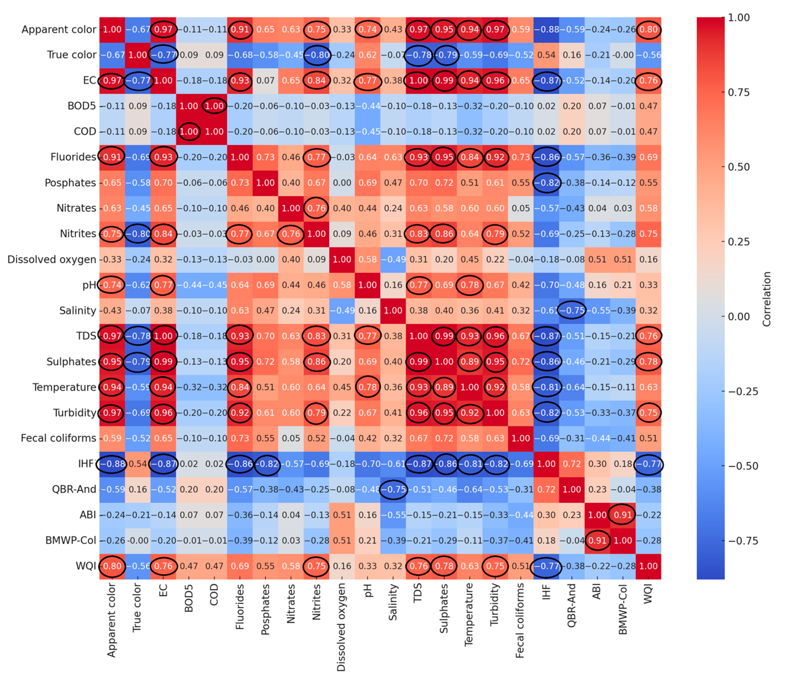
3.4.1. Correlation Patterns Among Physicochemical and Biological Variables

Figure 5 presents a heatmap of Pearson correlation coefficients, with statistically significant correlations (p < 0.01) highlighted by circles.

Apparent color showed significant positive correlations with electrical conductivity, fluorides, TDS, sulfates, and turbidity. Electrical conductivity was significantly correlated with TDS, sulfates, and turbidity. BOD₅ exhibited a significant correlation with COD. Fluorides were positively correlated with sulfates, while TDS showed significant relationships with sulfates and turbidity. The Fluvial Habitat Index (IHF) had statistically significant negative correlations of moderate-to-strong intensity (r between −0.81 and −0.88) with apparent color, electrical conductivity, fluorides, phosphates, TDS, sulfates, temperature, and turbidity. The Andean Biotic Index (ABI) demonstrated a strong, statistically significant positive correlation with the Biological Monitoring Working Party index adapted for Colombia (BMWP-Col). The Water Quality Index (WQI) showed a moderate negative correlation ($r$ = −0.77) with the Fluvial Habitat Index (IHF) and moderate positive correlations ($r$ between 0.75 and 0.80) with apparent color, electrical conductivity, nitrites, TDS, sulfates, and turbidity.

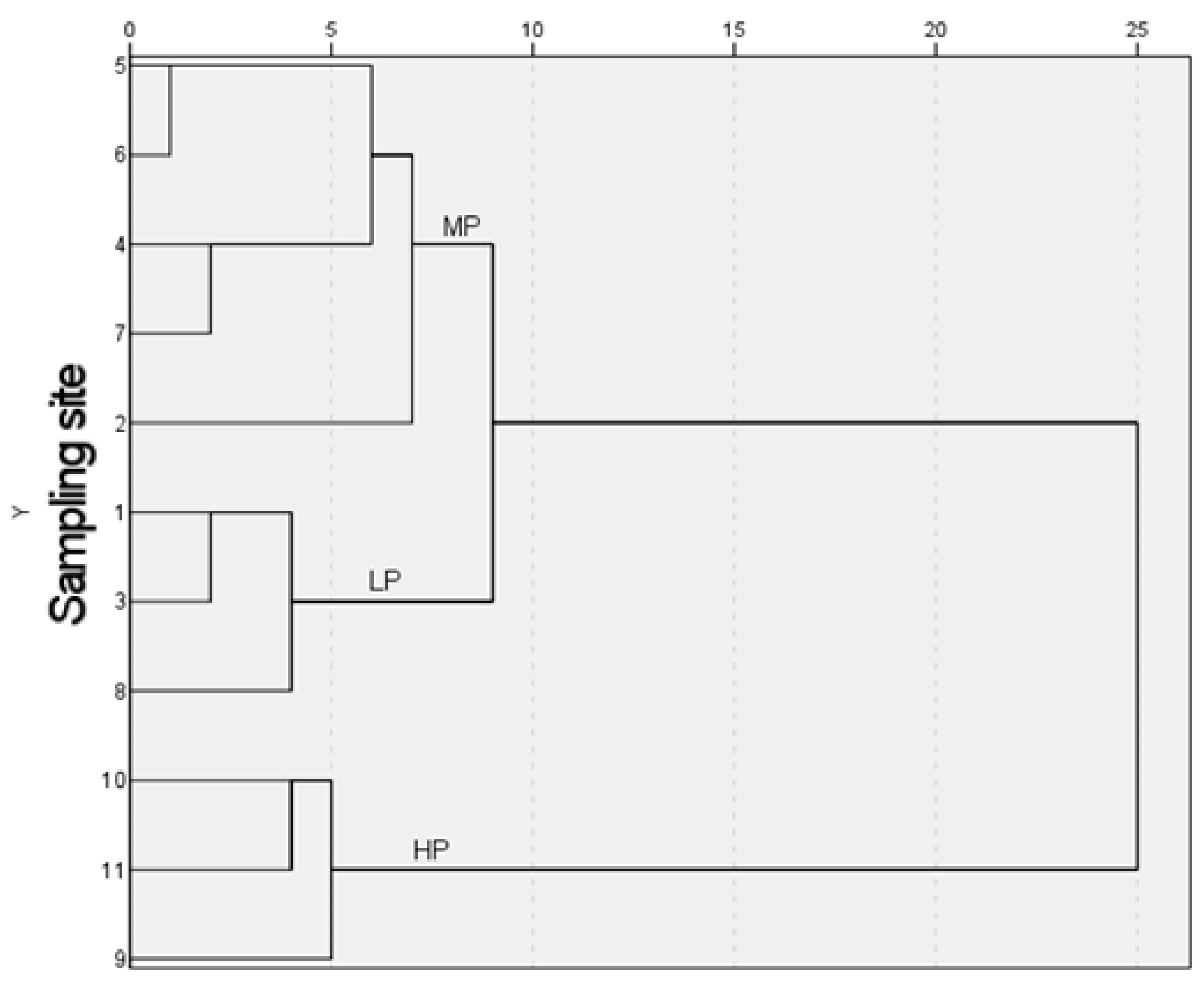
3.4.2. Cluster Analysis of Pollution Gradients

Sampling sites were classified based on their pollution levels using hierarchical cluster analysis that incorporated all evaluated physicochemical and microbiological parameters, along with the calculated indices.

To assess the consistency of the clustering outcome, a sensitivity analysis was conducted by reapplying the hierarchical cluster analysis using alternative linkage methods (single, complete, and average) and distance metrics (cityblock and correlation). The comparison revealed that, although minor variations occurred in the arrangement of specific sites, the overall structure remained stable across methods. This consistency reinforces the methodological reliability of the chosen configuration—Ward’s linkage and Euclidean distance—for classifying ecological conditions in the study area.

Additionally, the agglomeration coefficient curve was analyzed to determine the optimal number of clusters. A marked increase in the coefficient was observed between fusion stages 8 and 9 (from 5.91 to 10.00), indicating that merging beyond this point would combine ecologically distinct groups. This inflection point supported the selection of a three-cluster solution as the most representative configuration of the dataset (Figure 6).

Based on the dendrogram (Figure 6), three distinct clusters were identified, each representing a different level of environmental quality. Cluster I (less polluted—LP) includes points 1, 3, and 8, which exhibited favorable physicochemical conditions such as low-to-moderate levels of electrical conductivity, BOD₅, COD, and turbidity. These sites also recorded high scores in ecological indices (ABI, BMWP-Col, IHF, QBR-And), reflecting better habitat structure and biological integrity. Cluster II (moderately polluted—MP) comprises points 2, 4, 5, 6, and 7, which showed intermediate conditions. While some sites within this group exhibited relatively high values in individual structural indices—such as a high IHF value at point 6 and high QBR-And value at point 2—moderate concentrations of BOD₅, COD, and phosphates were also recorded, indicating mixed influence from natural and anthropogenic sources. Cluster III (highly polluted—HP) includes points 9, 10, and 11, which presented high values of electrical conductivity, BOD₅, COD, turbidity, TDS, and fecal coliforms. These sites also had low scores in both biotic and structural indices.

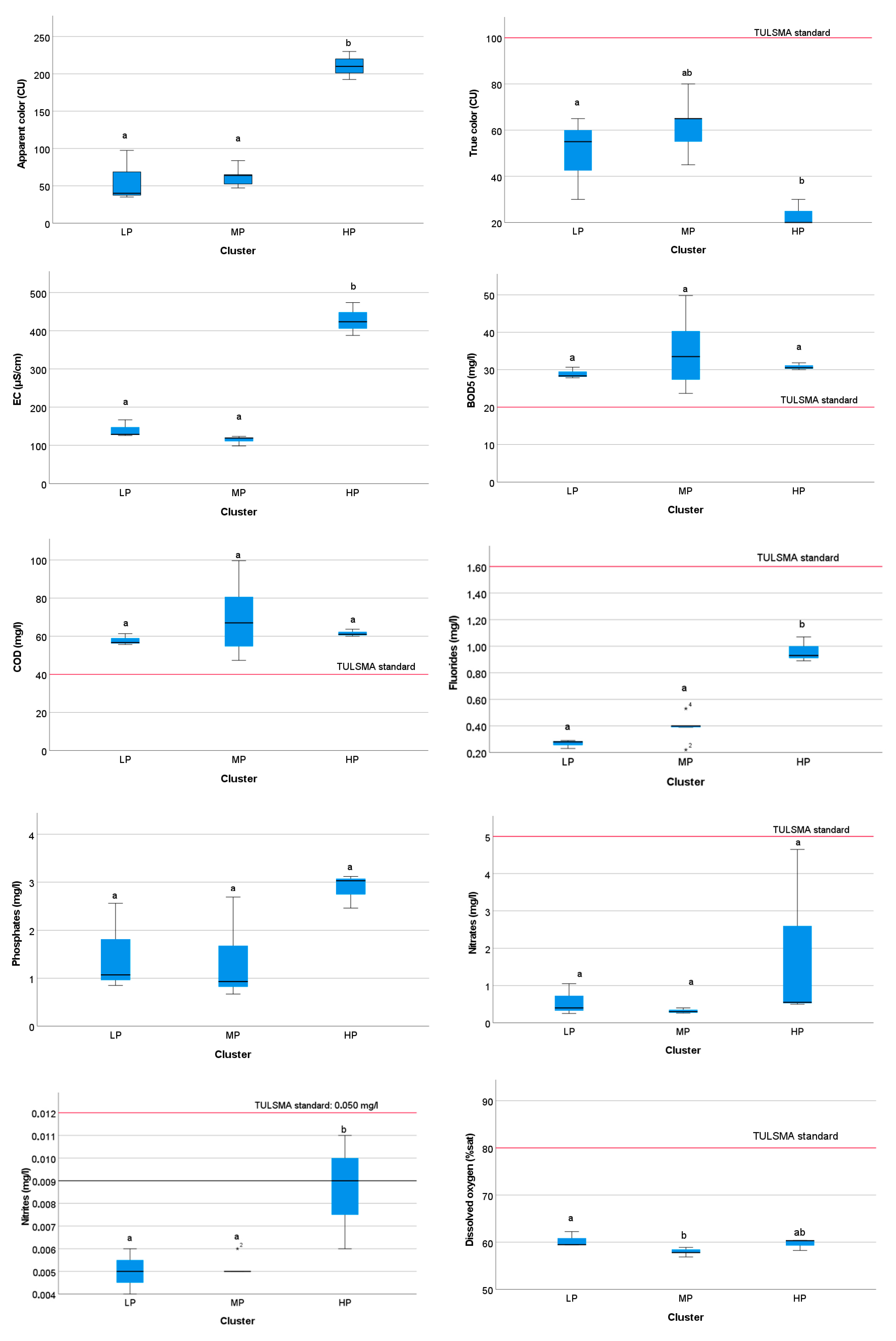
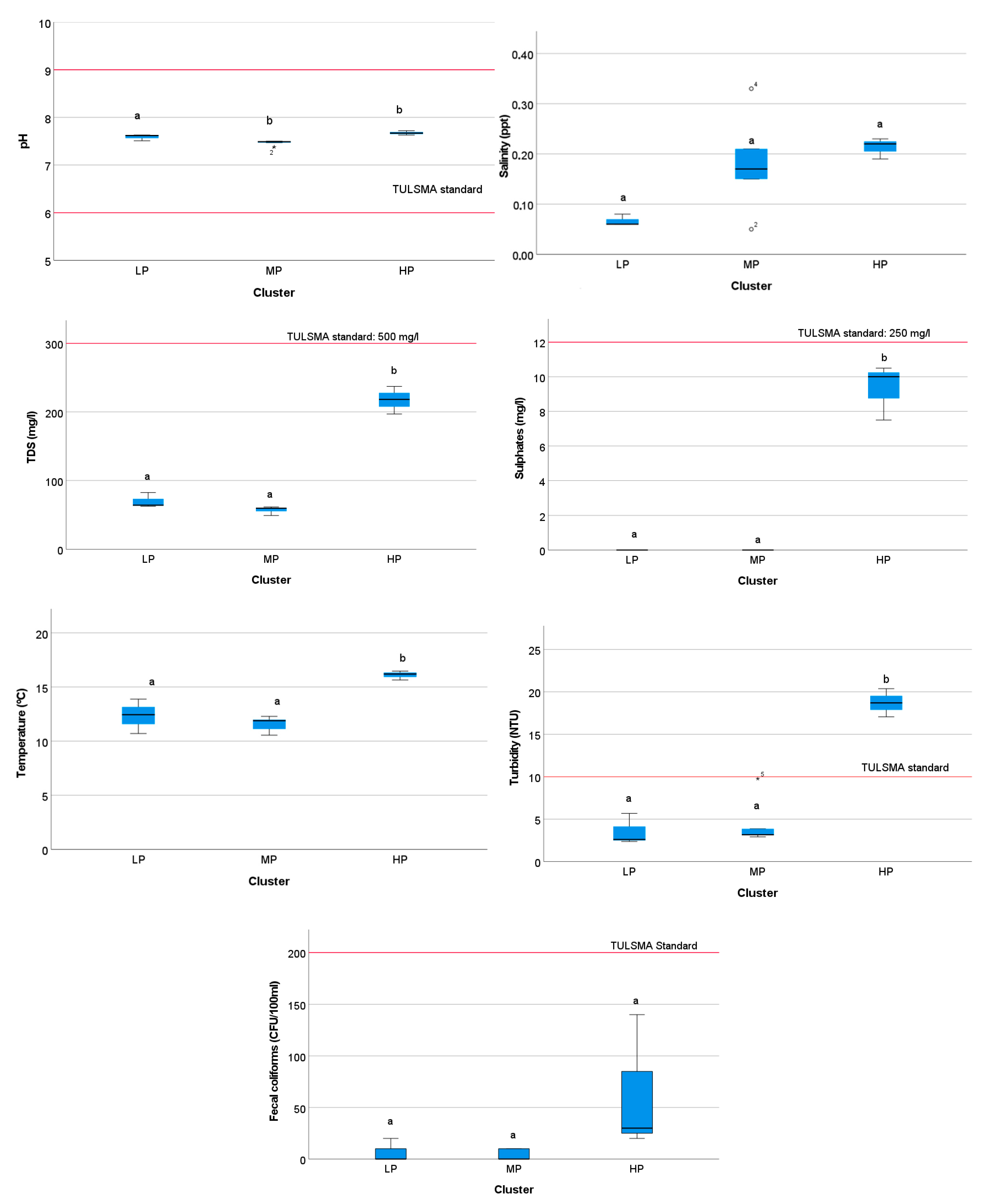
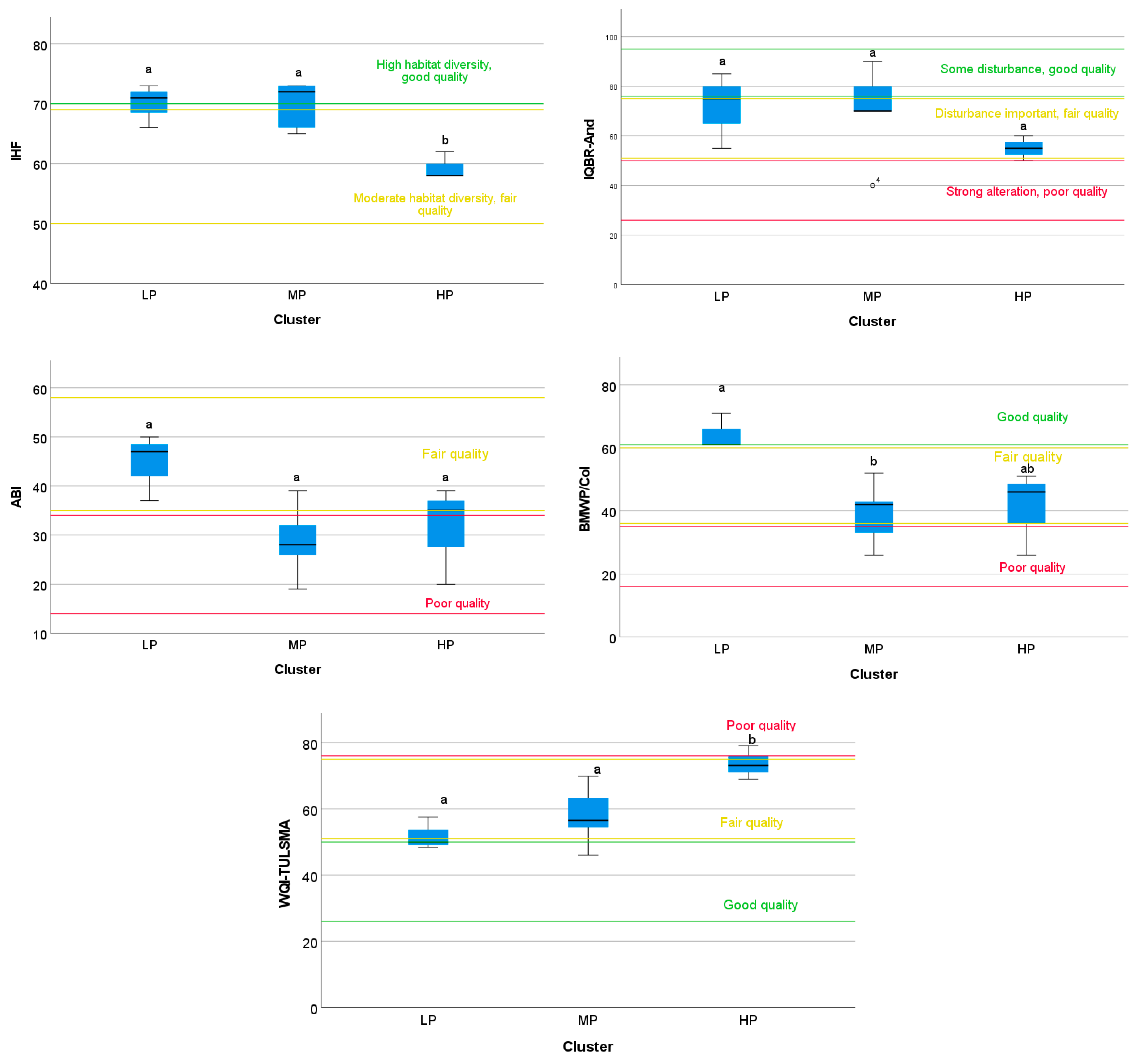
3.4.3. Spatial Variation in Environmental Quality by Cluster Group

Using the defined groups, boxplots were generated to visualize the results, revealing significant variations in the environmental quality of the sampling sites. The variations in each parameter are reflected in Figure 7, highlighting the differences among the groups (LP, MP, HP).

Apparent color values showed statistically significant differences among clusters (p < 0.05). The highest concentrations were recorded in the highly polluted (HP) group, with median values around 215 CU, while both the less polluted (LP) and moderately polluted (MP) clusters exhibited markedly lower and comparable values, with medians near 45 and 60 CU, respectively.

For true color, significant differences were also observed (p < 0.05). The HP cluster presented the lowest median values (≈25 CU), contrasting with the LP cluster (≈55 CU), which had higher concentrations. The MP cluster displayed intermediate values (≈65 CU) that did not differ significantly from either the LP or HP clusters.

Electrical conductivity varied significantly across clusters (p < 0.05), with the HP cluster exhibiting the highest median value (≈430 µS/cm). In contrast, the LP and MP clusters showed lower and statistically similar values (≈140 µS/cm and ≈120 µS/cm, respectively).

Biochemical oxygen demand (BOD₅) did not differ significantly among the clusters (p > 0.05). Median concentrations remained elevated in all three groups, with values around 29 mg/L (LP), 35 mg/L (MP), and 31 mg/L (HP), consistently exceeding the national regulatory standard of 20 mg/L.

Similarly, chemical oxygen demand (COD) showed no statistically significant differences (p > 0.05), with median values of 57 mg/L (LP), 68 mg/L (MP), and 61 mg/L (HP). These results also surpassed the TULSMA threshold of 40 mg/L.

In the case of fluorides, the HP group exhibited significantly higher concentrations (p < 0.05), with a median close to 0.95 mg/L. The LP and MP clusters reported lower and comparable values (≈0.28 mg/L and ≈0.40 mg/L, respectively), all within the permissible limit of 1.60 mg/L.

Phosphate levels did not differ significantly across clusters (p > 0.05), with median values of approximately 1.1 mg/L (LP), 1.0 mg/L (MP), and 3.0 mg/L (HP). Although higher in the HP cluster, the differences were not statistically significant.

Nitrate concentrations remained below the regulatory threshold of 5 mg/L at all sites, with no significant differences observed among clusters (p > 0.05). Median values were approximately 0.6 mg/L (LP), 0.4 mg/L (MP), and 2.5 mg/L (HP). In contrast, nitrite concentrations differed significantly (p < 0.05), with the highest median value recorded in the HP group (≈0.009 mg/L). The LP and MP clusters exhibited lower and statistically similar values around 0.005 mg/L, all within the acceptable limit of 0.050 mg/L.

Dissolved oxygen (% saturation) also showed statistically significant variation (p < 0.05). The MP group recorded the lowest values (median ≈ 58%), while the LP cluster had the highest (≈61%). The HP cluster exhibited intermediate values (≈60%), not differing significantly from either group.

Regarding pH, significant differences were identified (p < 0.05). The LP cluster showed slightly higher median values (≈7.65) compared to the MP (≈7.55) and HP (≈7.70) clusters, both of which remained within the acceptable range of 6-to-9.

Salinity did not present statistically significant differences across clusters (p > 0.05). Values remained relatively low, with medians around 0.07 ppt (LP), 0.18 ppt (MP), and 0.22 ppt (HP).

Total dissolved solids (TDS) differed significantly between clusters (p < 0.05). The HP group displayed the highest median value (≈220 mg/L), while the LP and MP clusters recorded lower and comparable concentrations (≈70 mg/L and ≈60 mg/L, respectively), all below the regulatory limit of 500 mg/L.

Sulfates were significantly higher in the HP cluster (p < 0.05), with median values around 10 mg/L. In contrast, the LP and MP clusters registered negligible concentrations, with no statistical difference between them.

Water temperature also differed significantly (p < 0.05). The HP cluster presented the highest median temperature (≈16 °C), whereas the LP and MP clusters recorded cooler conditions (≈12.5 °C and ≈12 °C, respectively), which did not differ significantly from each other.

Turbidity showed statistically significant differences among clusters (p < 0.05). The HP cluster had the highest levels (median ≈ 19 NTU), exceeding the regulatory standard of 10 NTU. The LP and MP clusters reported lower and statistically similar values (≈4 NTU).

Fecal coliform counts did not differ significantly among clusters (p > 0.05). All groups remained below the national threshold of 200 CFU/100 mL, with median values around 5–10 CFU/100 mL for the LP and MP clusters, and approximately 30 CFU/100 mL for the HP cluster.

A similar analysis was conducted using the five indices, comparing their results with the qualitative scale presented in Table 4. These findings are illustrated in Figure 8.

According to the Fluvial Habitat Index (IHF), the LP cluster presented values ranging from 67 to 72, with a median of 70. MP sites had a slightly wider range (66-to-74), also with a median of 70. No significant differences were found between these two clusters. In contrast, the HP cluster recorded lower values, between 58 and 61, with a median of 60, significantly differing from LP and MP groups (p < 0.05), and indicating a shift from “good” to “fair” habitat quality.

The QBR-And showed relatively high values for LP and MP clusters. LP sites ranged from 66 to 83, with a median of 77, while MP sites ranged from 76 to 90, with a median of 80. The HP cluster, however, presented notably lower values (median: 66; range: 63–68). Despite this trend, statistical analysis did not detect significant differences among the three groups (p ≥ 0.05), suggesting similar riparian vegetation quality across clusters, although with observable ecological degradation in HP sites.

In the ABI, LP sites recorded the highest scores, ranging from 43 to 50 (median: 47.5), followed by HP (median: 35; range: 29–38) and MP (median: 30; range: 20–38) sites. All three groups were categorized as having “fair” biological quality. Statistically, no significant differences were found among the clusters (p ≥ 0.05), despite the lower values observed in MP and HP sites.

The BMWP-Col exhibited clearer contrasts. LP sites showed values between 61 and 70 (median: 65), placing them in the “good” water quality category. MP sites had lower scores, ranging from 30 to 50 (median: 38), corresponding to “fair” quality, and were significantly different from LP sites (p < 0.05). HP sites ranged from 35 to 50, with a median of 45. These values were intermediate and did not differ significantly from either LP or MP sites, suggesting partial overlap in macroinvertebrate composition and water quality classification.

Finally, the WQI-TULSMA revealed statistically significant differences among clusters. LP sites had values between 50 and 57 (median: 53), and MP site values ranged from 49 to 68 (median: 61), both falling into the “fair” water quality category. The HP cluster showed higher WQI scores, from 75 to 79, with a median of 77, crossing the threshold into the “poor” quality classification. These values were significantly different from those in LP and MP sites (p < 0.05), indicating a pronounced degradation in physicochemical and microbiological parameters in HP sites.

4. Discussion

4.1. Physicochemical Parameters

The physicochemical results from the Columbe River micro-watershed revealed evident spatial patterns of degradation across the fluvial system. The highest BOD₅ and COD concentrations were recorded at P2 (BOD₅ = 49.8 mg/L, COD = 99.6 mg/L) and P10 (BOD₅ = 30.5 mg/L, COD = 61.0 mg/L), clearly exceeding the thresholds established by the Ecuadorian TULSMA regulation for aquatic life preservation (20 mg/L and 40 mg/L, respectively). These elevated values reflect chronic organic pollution, comparable to those reported in the Chumbao River (Peru) (BOD₅ = 105.38 mg/L) [42], and significantly higher than in relatively undisturbed Andean rivers, such as the Volcán River (Costa Rica) (3.93 mg/L) [19] and Yanaquincha River (Ecuador) (0.8 mg/L) [11]. Interestingly, P6 showed moderate BOD₅ levels (23.6 mg/L) but was classified as “good” in terms of habitat quality (IHF = 70), reinforcing the need for integrated, multimetric assessments.

Dissolved oxygen (DO) saturation ranged from 56.8% to 62.2%, well below the 80% threshold required by TULSMA. These hypoxic conditions likely result from high organic matter inputs, biological oxygen demand, and low turbulence in altered segments, trends consistent with observations in other tropical mountain systems [43,44].

The pH values were stable and neutral across all sampling points, ranging from 7.38 to 7.72. This pattern is consistent with values documented in the Orienco and Ichu streams [44,45], and reflects the buffering effect of bicarbonate weathering in high-altitude Andean systems [46]. Despite its limited sensitivity to pollution, pH provides insight into the geochemical stability and resilience of the system.

Electrical conductivity (EC) varied from 98.4 µS/cm at P2 to 473.8 µS/cm at P10, indicating substantial ion enrichment in more impacted sites. These values surpass those found in minimally disturbed rivers located in Cajas National Park (Ecuador) (70.5 µS/cm) [2] and approach levels reported in urban-impacted basins like the Tarqui River (Ecuador) (131.4 µS/cm) [2]. Elevated EC suggests the presence of untreated wastewater, agrochemical runoff, and leached solutes from deforested soils.

Turbidity peaked at P9 and P10 (18.7 and 20.3 NTU, respectively), exceeding the 10 NTU threshold set by TULSMA for aquatic life protection. These elevated values suggest substantial sediment input, likely driven by riparian vegetation loss, surface erosion, and unregulated runoff. Similar turbidity increases have been reported in deforested and livestock-impacted systems: for example, the Arroyo Grande River in Argentina exhibited turbidity levels of 59.7 NTU under similar land-use pressures [47]. In the Colombian Andes, deforestation for cattle grazing has been shown to cause soil compaction, reduce infiltration, and increase surface runoff, thereby elevating sediment loads in nearby water bodies [48].

Nitrate and nitrite concentrations generally remained within legal limits, with slightly elevated values at P10 (NO₃⁻ = 4.65 mg/L; NO₂⁻ = 0.011 mg/L). This pattern is consistent with denitrification processes in oxygen-depleted sediments and plant uptake in riparian zones [49,50]. Nonetheless, their presence in impacted areas suggests continuous input from diffuse sources such as agriculture, livestock, and domestic discharges [51].

Elevated phosphate concentrations at sampling points P9 (3.12 mg/L) and P10 (3.03 mg/L), coinciding with increased turbidity and organic matter levels, suggest significant phosphorus loading. This phenomenon is commonly observed in tropical watersheds, where phosphorus attaches to suspended particles, exacerbating eutrophication and disrupting biogeochemical cycles. For instance, studies have shown that phosphorus concentrations in water bodies rarely exceed 0.1 mg/L for inorganic phosphorus and 0.5 mg/L for total phosphorus [52]. However, during storm events, total particulate phosphorus (TPP) concentrations can increase significantly, with measurements averaging 118.4 μg P/L, which is 1.5-times higher than pre-storm riverine concentrations [53]. These elevated phosphorus levels, particularly when associated with suspended sediments, can lead to harmful algal blooms and oxygen depletion, as excessive phosphorus promotes the overgrowth of algae, subsequently affecting aquatic life and water quality [54].

Fecal coliform concentrations peaked at point P9, reaching 140 CFU/100 mL, substantially higher than at the other sampling sites. This elevated value suggests localized contamination, likely from untreated domestic wastewater or nearby livestock activity. In comparable rural settings, studies have shown that cattle access to stream banks can nearly double coliform levels in rivers [55]. In similar rural Andean settings, such as the Retamales River in Latacunga, reported fecal coliform levels were 66 and 41 CFU/100 mL, respectively, which are noticeably lower than those recorded at P9 in this study [17].

Hydrological conditions played a relevant role in the spatial distribution of pollutants. Sites with higher discharge, such as P3 (0.845 m³/s) and P11 (0.856 m³/s), did not necessarily present better physicochemical conditions. For instance, P11 exhibited a high EC and organic load despite its flow rate, illustrating that increased discharge is not sufficient to offset accumulated pollution [56]. Conversely, low-flow sites such as P1 (0.017 m³/s) and P7 (0.065 m³/s) were more prone to localized pollutant accumulation due to limited dilution capacity, a common pattern in low-flow systems with restricted turbulence. Duncan et al. (2024) examined the effects of droughts and heatwaves on freshwater quality globally, emphasizing that reduced discharge limits a river’s dilution capacity and can lead to increased concentrations of pollutants, particularly during extreme climatic events [57]. Similarly, Pakoksung et al. (2025) assessed seasonal water quality dynamics in the Chi-Mun River Basin, Thailand [58]. They found that contaminant levels were consistently higher during the dry season, a pattern linked to lower streamflows and reduced dilution [58].

4.2. Aquatic Diversity (ABI and BMWP-Col Indices)

Aquatic macroinvertebrate diversity in the Columbe River micro-watershed, assessed using the Andean Biotic Index (ABI) and BMWP-Col, revealed a marked gradient of ecological quality along the longitudinal profile of the watershed. The highest biotic integrity was observed at sites P3 and P1, with ABI scores of 50 and 48, and BMWP-Col values of 71 and 65, respectively. These values reflect the presence of pollution-sensitive taxa such as Perlidae, Baetidae, and Odontoceridae, which are indicators of good water quality and complex habitat structure [13,59]. Similar macroinvertebrate assemblages have been reported in reference headwater streams of the Guatapurí River in Colombia (BMWP-Col = 148) and the Yanaquincha River in the Ecuadorian Amazon (BMWP-Col = 72) [11,12].

In contrast, the most degraded sites—P9, P10, and P11—exhibited reduced biotic scores, with ABI values below 35 and BMWP-Col values below 50. These stations were dominated by tolerant taxa such as Chironomidae and Oligochaeta, consistent with high organic loads and habitat simplification. This assemblage structure mirrors conditions in heavily impacted systems like the downstream Guatapurí River (Colombia) (BMWP-Col = 130) [12], Antisana River Basin (ABI = 41) [10], and the lower Paute River, where sewage inputs and loss of structural complexity contribute to biological degradation [2].

Interestingly, inconsistencies in site classification emerged between the two biotic indices. For example, P4 and P7 were rated as “good” by the BMWP-Col (scores above 55), but received “poor” ratings under the ABI (scores below 30). This divergence is attributable to the differing design and sensitivity of the indices: the ABI prioritizes taxa endemic to high-elevation Andean systems, assigning higher weight to sensitive-but-less-diverse communities, while the BMWP-Col emphasizes overall family richness. Such discrepancies have been documented in other Andean catchments, including the Antisana and Cunas rivers, where index misalignment was linked to localized taxonomic dominance by moderately tolerant families [10,18].

Point P10 further exemplifies this pattern, as it was classified as “poor” by the WQI (score = 79) but recorded a moderate BMWP-Col score (50). This suggests either a lag in biological response or temporary recovery mechanisms within the macroinvertebrate community [60]. Additionally, hydrological conditions such as localized turbulence or substrate heterogeneity may support sensitive taxa even under moderate pollution levels [61].

Conversely, P8, a site with low pollution input and intermediate flow (0.156 m³/s), exhibited a lower ABI score (41) than expected for its chemical and structural conditions. This may be due to natural limitations in taxonomic richness associated with high-elevation streams, where faunal turnover and reduced colonization opportunities constrain biotic scores despite relatively intact habitats [1,13].

Overall, the biotic indices provided consistent evidence of ecological degradation in downstream segments and highlighted the role of anthropogenic stressors such as organic pollution, erosion, and riparian disturbance in shaping macroinvertebrate assemblages. However, the influence of natural variability—particularly hydrological dynamics—must be considered in interpreting index performance. Sites with moderate flow (e.g., P3) and minimal disturbance supported diverse and sensitive communities, reinforcing the importance of hydromorphological stability in maintaining ecological integrity. These findings are consistent with broader observations in the tropical Andes, where stream velocity, turbulence, and substrate complexity are critical in sustaining benthic diversity. In particular, Vázquez et al. (2020) [62] found that macroinvertebrate distribution in Andean rivers is closely linked to hydraulic factors such as flow velocity, turbulence, substrate complexity, and algal coverage. Their habitat suitability models, developed for key taxa in the Yanuncay River (Ecuador), revealed that sensitive groups like Baetodes, Simulium, and Anacroneuria thrive in fast, complex microhabitats. These findings highlight how changes in flow regimes or habitat simplification can significantly impact ecological integrity, even in chemically pristine streams.

4.3. Fluvial Habitat Structure (IHF and QBR Indices)

The fluvial habitat conditions in the Columbe River micro-watershed varied considerably across sampling points, with clear signs of structural degradation associated with human pressures. The Fluvial Habitat Index (IHF) ranged from 58 to 73, with the lowest scores recorded at P9 and P10. These values reflect habitat simplification due to sedimentation, riparian clearance, and flow homogenization. Similar IHF scores have been reported in degraded downstream segments of the Nonguén River in Chile (IHF = 45) [63] and the Paute River in Ecuador (IHF = 39) [2], where channelization and vegetation loss contribute to reduced physical complexity.

In contrast, the highest IHF values were observed at points P2, P3, and P6 (≥70), indicating more heterogeneous habitats with varied substrates, riffle frequency, and channel morphology. These sites featured better-developed instream habitats, including gravel bars, root systems, and variable depths, characteristics known to favor sensitive macroinvertebrate taxa [19,64]. The findings mirror upstream reaches of the Guatape (IHF = 79.7) and Volcán (IHF = 52) rivers, where similarly high IHF values have been linked to the presence of intact channel structures and well-preserved riparian buffers [19,64].

Riparian quality, assessed through the QBR-And, ranged from “poor” (score = 40) at P4 and P10 to “good” (score = 90) at P3. Lower values were associated with sites exhibiting extensive bank modification and vegetation replacement by crops or pasture. These patterns align with findings in the Guatapurí and Cunas rivers, where degraded riparian zones were linked to higher turbidity, elevated temperatures, and loss of habitat continuity [12,18]. Conversely, sites with dense canopy cover and native vegetation showed better biotic scores, confirming the critical role of riparian corridors in maintaining microclimatic stability and buffering surface runoff. This is consistent with broader ecological principles and recent studies demonstrating that riparian buffer width and vegetation structure significantly influence ecosystem attributes such as shading, organic matter input, sediment control, and biodiversity [65]. For instance, in Swedish boreal and temperate forests streams bordered by wider riparian buffers exhibited higher canopy cover and improved proxies for ecological functions like food provision and temperature regulation, especially in comparison with harvested sites lacking protective vegetation [66].

Despite some structural quality in specific points (e.g., P6, QBR-And = 78; IHF = 70), inconsistencies with chemical degradation indicators (e.g., high BOD₅ and turbidity) suggest that habitat condition alone does not guarantee ecological integrity when pollutant loads are excessive. This decoupling effect has also been observed in the Talala River (Ecuador), where persistent organic pollution masked the ecological benefits of partial vegetation recovery [8].

Hydrologically, sites with moderate-to-low discharge (e.g., P6 = 0.419 m³/s; P3 = 0.845 m³/s) supported more complex instream structures, possibly due to reduced erosive forces and a greater balance between sediment deposition and habitat formation. In contrast, high-flow points such as P11 (0.856 m³/s) showed low IHF scores (60), suggesting that increased discharge—when coupled with upstream disturbance—can lead to substrate instability and channel erosion. This pattern is consistent with findings by Kędzior et al. (2022) [67], who demonstrated that river incision significantly reduces the area of optimal habitat for macroinvertebrates. In such cases, even high environmental flow values may be insufficient to sustain biological integrity, as intense morphological degradation disrupts habitat complexity and limits faunal colonization.

4.4. Correlation Patterns Between Environmental and Biological Metrics

The correlation analysis (Figure 5) revealed statistically significant relationships (p < 0.01) between various physicochemical, structural, and biotic variables, offering insights into shared pollution sources and ecological responses in the Columbe River micro-watershed.

Apparent color showed strong positive correlations with electrical conductivity (EC; r = 0.97), fluorides (r = 0.91), total dissolved solids (TDS; r = 0.97), sulfates (r = 0.95), and turbidity (r = 0.97). These results indicate that apparent color in the Columbe River micro-watershed is closely linked to the presence of dissolved and suspended pollutants, many of which likely originate from domestic wastewater, erosion processes, and agricultural runoff. Similar associations have been observed in rivers of the Ecuadorian Amazon, where color metrics increased in parallel with ionic content and particulate load. Likewise, in the Talala River (Ecuador), Spearman correlation analysis from the period 2018–2019 revealed that apparent color was moderately associated with turbidity (r = 0.6), electrical conductivity (r = 0.4), iron (r = 0.4), and total coliforms (r = 0.6) [68], which also reflect pollutant inputs from erosion and untreated wastewater discharges.

The strong correlations between electrical conductivity (EC) and TDS (r = 0.99), sulfates (r = 0.93), and turbidity (r = 0.96) observed in the Columbe River align with findings from other studies. Thirumalini and Joseph (2008) [69] reported that EC explained up to 96% of TDS variability in natural waters, underscoring its usefulness as a proxy for ionic concentration. Similarly, Scott and Haggard (2019) [70] found elevated levels of TDS, turbidity, and sulfates in the downstream segments of the West Fork White River (USA), linked to anthropogenic land use.

The strong correlations between fluoride and sulfate (r = 0.95), and between fluoride and turbidity (r = 0.92), observed in the Columbe River suggest co-occurrence linked to shared sources such as leachates, erosion, and altered volcanic substrates. In the Cauca region (Colombia), fluoride concentrations reached up to 0.83 mg/L in the Cauca River, attributed to volcanic geology and surface runoff [71]. Similarly, in the Elqui River (Chile), sulfate-rich waters in the Andean zone reflected the oxidation of sulfide-bearing rocks and hydrothermal alteration, intensified by mining and weathering [72].

TDS showed strong positive correlations with sulfates (r = 0.99), temperature (r = 0.93), and turbidity (r = 0.96) in the Columbe River, highlighting the combined influence of dissolved and suspended matter in degraded reaches. While similar associations between TDS and electrical conductivity were observed in the Canuto (r = 0.95) and Carrizal (r = 0.99) rivers in coastal Ecuador, the relationship between TDS and temperature differed across sites [73]. In Canuto, temperature showed a weak positive correlation with TDS (r = 0.30), whereas in Carrizal the correlation was moderate and negative (r = −0.36). These contrasting patterns may reflect site-specific hydrological or thermal conditions influencing solute concentration dynamics, such as differential groundwater inputs, shading, or flow regulation.

Biochemical oxygen demand (BOD₅) and chemical oxygen demand (COD) showed a very strong correlation (r = 0.99) in the Columbe River, confirming their joint reliability as indicators of organic pollution. BOD₅ reflects microbial respiration driven by biodegradable organic matter, while COD includes both biodegradable and non-biodegradable oxidizable substances. This high association aligns with findings from wastewater treatment plants in Egypt, where the highest reported BOD₅/COD biodegradability index reached 0.88 in El Beheira governorate, illustrating a close relationship between both parameters under high organic load conditions [74].

The Fluvial Habitat Index (IHF) showed statistically significant negative correlations of moderate-to-strong intensity with several physicochemical variables: apparent color (r = −0.88), EC (r = −0.87), fluorides (r = −0.86), phosphates (r = −0.82), TDS (r = −0.87), sulfates (r = −0.86), temperature (r = −0.81), and turbidity (r = −0.82). These results underscore the inverse relationship between structural habitat quality and physicochemical degradation. Similar patterns have been reported by Echeverría-Sáenz et al. (2022) [19] and Munné et al. (2003) [38], who highlighted that increased sedimentation, thermal load, and ionic concentration contribute to habitat homogenization and degradation.

Importantly, biotic indices demonstrated internal consistency. The Andean Biotic Index (ABI) showed a strong positive correlation with the BMWP-Col (r = 0.91), confirming a high degree of congruence in their classification of ecological status based on macroinvertebrate assemblages. This supports earlier findings by Ríos-Touma et al. (2014) [13], who noted that while each index has its strengths and taxonomic nuances, both tend to converge in detecting pollution gradients when family richness is adequate.

The Water Quality Index (WQI) showed a moderate negative correlation with IHF (r = −0.77), supporting the notion that declines in structural complexity coincide with worsening chemical quality. This pattern is consistent with findings from the Maranhão Amazon, where Braga et al. (2022) [75] reported that sites with elevated turbidity, nutrient loads, and microbiological contamination—particularly during the rainy season—were associated with reduced WQI scores, as revealed through multivariate statistical analysis. Although habitat variables were not directly measured, the clustering of degraded chemical conditions in specific sites suggests underlying structural deterioration. Similarly, in the Paute River Basin (Ecuador), Sotomayor et al. (2016) [76] found that riparian vegetation and streambed heterogeneity were the strongest predictors of better macroinvertebrate-based water quality classes, while poor habitat structure coincided with higher levels of pollutants such as fecal coliforms and thermal stress.

4.5. Spatial Distribution of Physicochemical and Biological Indices

The hierarchical cluster analysis clearly distinguished three ecological conditions across the Columbe River micro-watershed: less polluted (LP: P1, P3, P8), moderately polluted (MP: P2, P4, P5, P6, P7), and highly polluted (HP: P9, P10, P11). This classification was statistically supported and allowed the spatial differentiation of the system based on pollution intensity, habitat integrity, and biological responses.

LP sites exhibited the best ecological conditions. They were characterized by high ABI scores (median = 47.5), elevated BMWP-Col values (median = 65), low turbidity (<5 NTU), and good fluvial habitat structure (IHF median = 70). For example, P3, with a flow of 0.845 m³/s, registered some of the highest ABI (50) and IHF (73) values, suggesting that a combination of moderate hydrological stability, minimal pressure, and habitat complexity can support sensitive macroinvertebrate assemblages even under relatively low base flows. These conditions resemble those described in upstream segments of the Guatapurí River (BMWP-Col = 148, QBR = 80) [12] and the Yanaquincha River (BMWP-Col = 72) [11], confirming their status as local reference conditions.

MP sites showed intermediate values and mixed signals of degradation. For example, P6 had an IHF of 70 and QBR-And of 78, suggesting relatively good habitat structure, but simultaneously presented BOD₅ = 23.6 mg/L and moderate turbidity. Similarly, P2 had the highest COD (99.6 mg/L) and BOD₅ (49.8 mg/L), despite moderate IHF (68), underscoring the complex dynamics between structural features and pollution inputs. These findings reflect partial degradation, often due to diffuse pollution and localized habitat disturbance. Comparable transitional conditions have been reported in the mid-reaches of the Guatape and Cunas rivers, where moderate flows and agricultural runoff produce heterogeneity in ecological indicators [18,64].

HP sites were consistently associated with high pollutant concentrations and biological impoverishment. For example, P10 and P11 exhibited elevated BOD₅ (30.5 and 26.1 mg/L), COD (61.0 and 54.0 mg/L), turbidity (>18 NTU), and conductivity (>400 µS/cm), along with low IHF scores (58 and 60). Biologically, these sites were dominated by tolerant taxa such as Chironomidae and Oligochaeta, and had ABI scores below 35, indicating a severely altered ecological status. Similar conditions were reported in the Paute River Basin (Ecuador), where the most degraded sites (C3 class) were associated with low habitat quality and a simplified benthic community dominated by pollution-tolerant groups, underpinned largely by the loss of riparian vegetation and instream heterogeneity [76]. In the Portoviejo River (Ecuador), Nguyen et al. (2015) [77] found that macroinvertebrate community composition shifted markedly in response to rising conductivity, with tolerant taxa becoming dominant at sites exceeding 1430 µS/cm, supporting the link between ionic concentration and biological simplification. Likewise, Banda et al. (2022) [78] observed that high conductivity and organic enrichment in a tropical wetland led to reductions in community diversity and the prevalence of tolerant macroinvertebrate assemblages. These consistent findings across different systems reinforce the interpretation that elevated BOD₅, COD, turbidity, and conductivity—coupled with low structural integrity—underpin ecological degradation and favor dominance by tolerant taxa, as observed in the Columbe River.

Interestingly, P11—despite its relatively high discharge (0.856 m³/s)—remained in the high-pollution group, underscoring that increased flow alone does not mitigate the impacts of pollution when structural degradation and external inputs are severe. This finding aligns with the work of Simon and Rinaldi (2006) [79], who demonstrated that in incised or hydromorphologically unstable channels, increases in stream power due to higher flows can actually exacerbate erosion and habitat loss when boundary resistance is low. Similarly, Santikari and Murdoch (2020) [80] observed that in urbanizing watersheds, elevated stormflows—often several times greater than in undisturbed systems—did not prevent sediment surges and water quality deterioration, especially when vegetation and soil stability were compromised. Moreover, Cashman et al. (2023) [81] emphasized that degraded physical habitat is not merely a sediment issue, but is tightly linked to altered flow regimes. Their findings indicate that even in systems with high discharge, the absence of hydromorphic heterogeneity and riparian stability leads to declines in habitat quality. Taken together, these studies support the notion that flow magnitude, in isolation, is insufficient to buffer the ecological impacts of structural and chemical degradation, an interpretation confirmed by the impaired status of P11 in the Columbe River.

In contrast, P1, with the lowest flow (0.017 m³/s), maintained high biological and structural index values, although it showed elevated BOD₅ (27.8 mg/L). This suggests that headwater segments, despite their lower dilution capacity, can maintain ecological integrity when pressure levels are minimal and riparian buffers are preserved. Similar dynamics were observed in the upstream Volcán and Guatapurí rivers, where intact vegetation and minimal land use resulted in higher ecological scores despite natural limitations in flow and substrate availability [12,19].

4.6. Implications for Sustainability and Integrated Watershed Management

The findings from the Columbe River micro-watershed highlight the urgent need for integrated watershed management in high-Andean regions undergoing rapid land-use transformation. The observed decline in water quality, habitat structure, and macroinvertebrate diversity reflects broader sustainability challenges common in mountain systems where environmental regulation is often limited or poorly enforced. Similar conclusions have been drawn in other highland regions. For example, Haq et al. (2021) [82] demonstrated that riparian zones in the Kashmir Himalaya sustain high floristic and functional diversity, which is essential for ecological resilience. Likewise, Mosquera et al. (2023) [83] emphasized that while páramo ecosystems are critical for hydrological regulation, they lack integrated research on vegetation–water interactions, highlighting the need for interdisciplinary management strategies.

The relationships observed in the Columbe River micro-watershed between land use and aquatic ecosystem health are consistent with broader empirical evidence. Cortes et al. (2013) [84] showed that land-use patterns—particularly urbanization at local scales—are strong predictors of ecological quality in rivers, as reflected by macroinvertebrate-based bioindicators. Their study highlighted the importance of integrating biotic responses with spatially explicit land-use data to guide effective river management. Similarly, Brumberg et al. (2021) [85] found that riparian buffer length, more than width, had the greatest influence on water quality in agricultural landscapes of southern Costa Rica, suggesting that even narrow, but continuous, riparian buffers can significantly improve water quality where full-width restoration is impractical.

Beyond biophysical strategies, institutional mechanisms such as payment for ecosystem services (PES) offer promising tools to incentivize upstream conservation. Izquierdo-Tort et al. (2022) [20], in a randomized trial in Mexico, showed that requiring full-parcel enrollment in PES contracts reduced deforestation by 41% and quadrupled cost-effectiveness compared to traditional schemes. These findings underscore how strategic adjustments in PES design can substantially enhance environmental outcomes. Taken together, these studies reinforce the need to combine ecological indicators, spatial planning, and institutional innovation to advance sustainability in rapidly transforming Andean watersheds.

Although this study offers a detailed assessment of ecological integrity and water quality in a high-Andean micro-watershed, certain limitations should be acknowledged. First, macroinvertebrate sampling was conducted during a single season, which may not fully capture temporal variability in community composition influenced by hydrological fluctuations (e.g., [1,2]). Additionally, the use of indices such as the ABI and BMWP-Col—although regionally adapted—relies on fixed tolerance scores that may oversimplify the ecological responses to multiple and interacting stressors (e.g., [3,4]). Moreover, while the selection of 11 sampling points aimed to ensure representativeness, the spatial coverage may not fully reflect the heterogeneity of the watershed, particularly in transitional zones or ephemeral tributaries.

Future research should incorporate multi-seasonal monitoring to better account for seasonal ecological variation and improve the reliability of biotic assessments (e.g., [5]). Integrating molecular tools, such as DNA barcoding, could enhance taxonomic resolution and enable the detection of cryptic diversity often overlooked by conventional methods [6]. Modeling scenarios involving land-use change, climate variability, and restoration actions may also provide strategic insights for long-term watershed planning [7]. Furthermore, expanding participatory monitoring with local communities could enhance data coverage and foster stronger stakeholder involvement in conservation strategies [8].

5. Conclusions

This study provides clear evidence that anthropogenic pressures—particularly agriculture, livestock, and untreated domestic discharges—are major drivers of ecological degradation in the Columbe River micro-watershed. These pressures contribute to the physicochemical alteration in aquatic systems and are closely linked to reduced macroinvertebrate diversity, declining water quality, and deteriorated fluvial habitat structure.

The results show that elevated concentrations of BOD₅, COD, and electrical conductivity, alongside low values of habitat quality indices (IHF and QBR-And), are strongly associated with the dominance of tolerant taxa such as Oligochaeta and Chironomidae. This shift in community composition reflects not only site-specific disturbances but also cumulative basin-wide impacts that compromise ecosystem functionality.

The combined degradation of chemical and structural conditions leads to ecological fragmentation and loss of biodiversity in high-Andean aquatic systems. These findings underscore the need for fluvial restoration strategies that are grounded in empirical data and consider both ecological and social dimensions. Restoring habitat complexity, improving water quality, and enhancing ecological connectivity will be essential to safeguard the ecological integrity and service provision of these vulnerable mountain ecosystems. In this context, the adoption of integrated watershed management approaches supports long-term sustainability by aligning conservation actions with land-use planning, local livelihoods, and climate resilience, which are fundamental components for advancing Sustainable Development Goals (SDGs) in rural Andean regions.

References

1. Villamarín, C.; Prat, N.; Rieradevall, M. Physical, chemical and hydromorphological characterization of Ecuador and Peru tropical highland Andean rivers. Lat. Am. J. Aquat. Res. 2014, 42, 1072–1086. [Google Scholar] [CrossRef]
2. Hampel, H.; Vázquez, R.F.; González, H.; Acosta, R. Evaluating the ecological status of fluvial networks of tropical Andean catchments of Ecuador. Water 2023, 15, 1742. [Google Scholar] [CrossRef]
3. Fierro, P.; Bertrán, C.; Tapia, J.; Hauenstein, E.; Peña-Cortés, F.; Vergara, C.; Cerna, C.; Vargas-Chacoff, L. Effects of local land-use on riparian vegetation, water quality, and the functional organization of macroinvertebrate assemblages. Sci. Total Environ. 2017, 609, 724–734. [Google Scholar] [CrossRef] [PubMed]
4. Rodríguez-Morales, M.; Acevedo-Novoa, D.; Machado, D.; Ablan, M.; Dugarte, W.; Dávila, F. Ecohydrology of the Venezuelan páramo: Water balance of a high Andean watershed. Plant Ecol. Divers. 2019, 12, 573–591. [Google Scholar] [CrossRef]
5. Espinosa, J.; Rivera, D. Variations in water resources availability at the Ecuadorian páramo due to land-use changes. Environ. Earth Sci. 2016, 75, 1173. [Google Scholar] [CrossRef]
6. Patiño, S.; Hernández, Y.; Plata, C.; Domínguez, I.; Daza, M.; Oviedo-Ocaña, R.; Ochoa-Tocachi, B.F. Influence of land use on hydro-physical soil properties of Andean páramos and its effect on streamflow buffering. Catena 2021, 202, 105227. [Google Scholar] [CrossRef]
7. Villa-Achupallas, M.; Rosado, D.; Aguilar, S.; Galindo-Riaño, M.D. Water quality in the tropical Andes hotspot: The Yacuambi river (southeastern Ecuador). Sci. Total Environ. 2018, 633, 50–58. [Google Scholar] [CrossRef]
8. Salazar Flores, C.; Zambrano, C.; Parreno, C. Microbiological assessment of the quality of water supplied to the Latacunga water treatment plant (Republic of Ecuador). Int. Res. J. 2023, 2, 128. [Google Scholar] [CrossRef]
9. Campo, Y.M.; Rebolledo, M.I.C.; Londoño, A.M.J. Comparison of water quality between two Andean rivers by using the BMWP/COL and ABI indices. Acta Biol. Colomb. 2019, 24, 1–9. [Google Scholar] [CrossRef]
10. Cabrera-García, S.; Goethals, P.L.M.; Lock, K.; Domínguez-Granda, L.; Villacís, M.; Galárraga-Sánchez, R.; Van der Heyden, C.; Forio, M.A.E. Taxonomic and feeding trait-based analysis of macroinvertebrates in the Antisana River Basin (Ecuadorian Andean Region). Biology 2023, 12, 1386. [Google Scholar] [CrossRef]
11. Vargas-Tierras, T.; Suárez-Cedillo, S.; Morales-León, V.; Vargas-Tierras, Y.; Tinoco-Jaramillo, L.; Viera-Arroyo, W.; Vásquez-Castillo, W. Ecological River Water Quality Based on Macroinvertebrates Present in the Ecuadorian Amazon. Sustainability 2023, 15, 5790. [Google Scholar] [CrossRef]
12. Herrera-Martínez, J.R.; Navarro-Sining, B.A.; Torres-Cervera, K.P.; Martínez-García, N.; Royero-Ibarra, A.; Cahuana-Mojica, A. Determinación de los índices BMWP/COL, QBR, IHF e ICO en Valledupar, Colombia. Rev. Politéc. 2022, 18, 98–109. [Google Scholar] [CrossRef]
13. Ríos-Touma, B.; Acosta, R.; Prat, N. The Andean Biotic Index (ABI): Revised tolerance to pollution values for macroinvertebrate families and index performance evaluation. Rev. Biol. Trop. 2014, 62, 249–273. [Google Scholar] [CrossRef]
14. Roldán, G. La Bioindicación de la Calidad del Agua en Colombia: Propuesta para el uso del Método BMWP-COL; Editorial Universidad de Antioquia: Medellín, Colombia, 2003. [Google Scholar]
15. Pardo, I.; Álvarez, M.; Casas, J.J.; Moreno, J.L.; Vivas, S.; Bonada, N.; Alba-Tercedo, J.; Jaimez-Cuéllar, P.; Moya, G.; Prat, N.; et al. El hábitat de los ríos mediterráneos: Diseño de un índice de diversidad de hábitat. Limnetica 2002, 21, 115–132. [Google Scholar] [CrossRef]
16. Acosta, R.; Ríos, B.; Rieradevall, M.; Prat, N. Propuesta de un protocolo de evaluación de la calidad ecológica de ríos andinos (C.E.R.A.) y su aplicación en dos cuencas en Ecuador y Perú. Limnetica 2009, 28, 35–64. [Google Scholar] [CrossRef]
17. Salazar Flores, C.A.; Kurbatova, A.I.; Mikhaylichenko, K.Y.; Barannikova, S.I. Comprehensive water quality assessment of surface sources in the city of Latacunga and the canton Pedro Vicente Maldonado in Ecuador. RUDN J. Ecol. Life Saf. 2023, 31, 251–264. [Google Scholar] [CrossRef]
18. Custodio, M.; Chávez, E. Quality of the aquatic environment of high Andean rivers evaluated through environmental indicators: A case of the Cunas River, Peru. Ingeniare 2019, 27, 396–409. [Google Scholar] [CrossRef]
19. Echeverría-Sáenz, S.; Ugalde-Salazar, R.; Guevara-Mora, M.; Quesada-Alvarado, F.; Ruepert, C. Ecological Integrity Impairment and Habitat Fragmentation for Neotropical Macroinvertebrate Communities in an Agricultural Stream. Toxics 2022, 10, 346. [Google Scholar] [CrossRef]
20. Izquierdo-Tort, S.; Jayachandran, S.; Saavedra, S. Redesigning payments for ecosystem services to increase cost-effectiveness. Nat. Commun. 2024, 15, 9252. [Google Scholar] [CrossRef]
21. Vasseur, L.; Andrade, A. Using the Red List of Ecosystems and the Nature-based Solutions Global Standard as an integrated process for climate change adaptation in the Andean high mountains. Philos. Trans. R. Soc. B 2024, 379, 20220326. [Google Scholar] [CrossRef]
22. GAD de la Parroquia Columbe. Plan de Desarrollo y Ordenamiento Territorial de la Parroquia Columbe 2019–2023. Available online: https://es.slideshare.net/slideshow/pdotcolumbe2020pdf/252797787 (accessed on 25 January 2025).
23. GAD de la Provincia de Chimborazo. Plan de Desarrollo y Ordenamiento Territorial de la Provincia de Chimborazo 2019–2023. Available online: https://chimborazo.gob.ec/principal/wp-content/uploads/2022/06/PDOT.pdf (accessed on 24 January 2025).
24. Santillán, G. Macroinvertebrados Acuáticos Como Bioindicadores de Calidad de Agua en la Microcuenca Columbe, Cantón Colta. Master’s Thesis, Universidad Nacional de Chimborazo, Riobamba, Ecuador, 2024. Available online: http://dspace.unach.edu.ec/handle/51000/13571 (accessed on 25 January 2025).
25. Damanik-Ambarita, M.N.; Lock, K.; Boets, P.; Everaert, G.; Nguyen, T.H.T.; Forio, M.A.E.; Musonge, P.L.S.; Suhareva, N.; Bennetsen, E.; Landuyt, D.; et al. Ecological water quality analysis of the Guayas River basin (Ecuador) based on macroinvertebrates indices. Limnologica 2016, 57, 27–59. [Google Scholar] [CrossRef]
26. Paller, M.H.; Kosnicki, E.; Prusha, B.A.; Fletcher, D.E.; Sefick, S.A.; Feminella, J.W. Development of an Index of Biotic Integrity for the Sand Hills Ecoregion of the Southeastern United States. Trans. Am. Fish. Soc. 2017, 146, 112–127. [Google Scholar] [CrossRef]
27. Edegbene, A.O.; Akamagwuna, F.C.; Odume, O.N.; Arimoro, F.O.; Edegbene, O.T.T.; Akumabor, E.C.; Ogidiaka, E.; Kaine, E.A.; Nwaka, K.H. A Macroinvertebrate-Based Multimetric Index for Assessing Ecological Condition of Forested Stream Sites Draining Nigerian Urbanizing Landscapes. Sustainability 2022, 14, 11289. [Google Scholar] [CrossRef]
28. Raven, P.J.; Holmes, N.T.H.; Charrier, P.; Dawson, F.H.; Naura, M.; Boon, P.J. Towards a harmonized approach for hydromorphological assessment of rivers in Europe: A qualitative comparison of three survey methods. Aquat. Conserv. 2002, 12, 405–424. [Google Scholar] [CrossRef]
29. Fernández, D.; Barquín, J.; Raven, P. A review of river habitat characterisation methods: Indices vs. characterisation protocols. Limnetica 2011, 30, 217–234. [Google Scholar] [CrossRef]
30. Uddin, M.G.; Nash, S.; Olbert, A.I. A review of water quality index models and their use for assessing surface water quality. Ecol. Indic. 2021, 122, 107218. [Google Scholar] [CrossRef]
31. Lukhabi, D.K.; Mensah, P.K.; Asare, N.K.; Pulumuka-Kamanga, T.; Ouma, K.O. Adapted Water Quality Indices: Limitations and Potential for Water Quality Monitoring in Africa. Water 2023, 15, 1736. [Google Scholar] [CrossRef]
32. Hanna Instruments. HI98194 Multiparameter Waterproof Meter. Available online: https://www.hannainstruments.co.uk/multi-parameter-devices/2147-hi-98194-multiparameter-waterproof-meter (accessed on 10 January 2025).
33. Valladares Pogo, V. Evaluación Ecológica del río Columbe. Bachelor’s Thesis, Escuela Superior Politécnica de Chimborazo (ESPOCH), Riobamba, Ecuador, 2024. Available online: http://dspace.espoch.edu.ec/handle/123456789/23192 (accessed on 25 January 2025).
34. Instituto Privado de Investigación Sobre Cambio Climático (ICC). Manual de Medición de Caudales; Guatemala. 2017. Available online: https://icc.org.gt/wp-content/uploads/2023/03/064.pdf (accessed on 30 January 2025).
35. Ministerio de Agricultura del Perú. Manual de Hidrometría; Ministerio de Agricultura del Perú: Lima, Perú, 2005. [Google Scholar]
36. Pence, R.A.; Cianciolo, T.R.; Drover, D.R.; McLaughlin, D.L.; Soucek, D.J.; Timpano, A.J.; Zipper, C.E.; Schoenholtz, S.H. Comparison of benthic macroinvertebrate assessment methods along a salinity gradient in headwater streams. Environ. Monit. Assess. 2021, 193, 765. [Google Scholar] [CrossRef]
37. Getachew, M.; Mulat, W.L.; Mereta, S.T.; Gebrie, G.S.; Kelly-Quinn, M. Refining benthic macroinvertebrate kick sampling protocol for wadeable rivers and streams in Ethiopia. Environ. Monit. Assess. 2022, 194, 196. [Google Scholar] [CrossRef]
38. Munné, A.; Prat, N.; Solà, C.; Bonada, N.; Rieradevall, M. A simple field method for assessing the ecological quality of riparian habitat in rivers and streams: QBR index. Aquat. Conserv. 2003, 13, 147–163. [Google Scholar] [CrossRef]
39. Instituto Geográfico Militar del Ecuador (IGM). Capas de Información Geográfica del IGM (Codificación UTF-8). Available online: http://www.geoportaligm.gob.ec/portal/index.php/descargas/cartografia-de-libre-acceso/registro/ (accessed on 27 January 2025).
40. Gaagai, A.; Aouissi, H.A.; Bencedira, S.; Hinge, G.; Athamena, A.; Heddam, S.; Gad, M.; Elsherbiny, O.; Elsayed, S.; Eid, M.H.; et al. Application of Water Quality Indices, Machine Learning Approaches, and GIS to Identify Groundwater Quality for Irrigation Purposes: A Case Study of Sahara Aquifer, Doucen Plain, Algeria. Water 2023, 15, 289. [Google Scholar] [CrossRef]
41. Yang, J.; Lv, J.; Liu, Q.; Nan, F.; Li, B.; Xie, S.; Feng, J. Seasonal and spatial patterns of eukaryotic phytoplankton communities in an urban river based on marker gene. Sci. Rep. 2021, 11, 23147. [Google Scholar] [CrossRef] [PubMed]
42. Ramos-Pacheco, B.S.; Choque-Quispe, D.; Ligarda-Samanez, C.A.; Solano-Reynoso, A.M.; Choque-Quispe, Y.; Aguirre Landa, J.P.; Agreda Cerna, H.W.; Palomino-Rincón, H.; Taipe-Pardo, F.; Zamalloa-Puma, M.M.; et al. Water Pollution Indexes Proposal for a High Andean River Using Multivariate Statistics: Case of Chumbao River, Andahuaylas, Apurímac. Water 2023, 15, 2662. [Google Scholar] [CrossRef]
43. Huang, Y.; Yang, C.; Wen, C.; Wen, G. S-type Dissolved Oxygen Distribution along Water Depth in a Canyon-shaped and Algae Blooming Water Source Reservoir: Reasons and Control. Int. J. Environ. Res. Public Health 2019, 16, 987. [Google Scholar] [CrossRef]
44. Sinche, F.; Cabrera, M.; Vaca, L.; Segura, E.; Carrera, P. Determination of the Ecological Water Quality in the Orienco Stream Using Benthic Macroinvertebrates in the Northern Ecuadorian Amazon. Integr. Environ. Assess. Manag. 2022, 11, e4666. [Google Scholar] [CrossRef]
45. Sánchez-Araujo, V.; Portuguez-Maurtua, M.; Palomino-Pastrana, P.; Escobar-Soldevilla, M.; Saez Huaman, W.; Chávez-Araujo, E.; Contreras López, E. Water Quality Index and Health Risks in a Peruvian High Andean River. Ecol. Eng. Environ. Technol. 2024, 25, 301–315. [Google Scholar] [CrossRef]
46. Torres, M.A.; West, A.J.; Clark, K.E.; Paris, G.; Bouchez, J.; Ponton, C.; Feakins, S.J.; Galy, V.; Adkins, J.F. The acid and alkalinity budgets of weathering in the Andes–Amazon system: Insights into the erosional control of global biogeochemical cycles. Earth Planet. Sci. Lett. 2016, 450, 381–391. [Google Scholar] [CrossRef]
47. Granitto, M.; Lopez, M.E.; Bursztyn Fuentes, A.L.; Maluendez Testoni, M.C.; Rodríguez, P. Relationship between riparian zones and water quality in the main watersheds of Ushuaia City, Tierra del Fuego (Argentina). Ecol. Process. 2025, 14, 18. [Google Scholar] [CrossRef]
48. Vásquez-Velásquez, G. Headwaters Deforestation for Cattle Pastures in the Andes of Colombia and Its Implications for Soils Properties and Hydrological Dynamic. Open J. For. 2016, 6, 337–347. [Google Scholar] [CrossRef]
49. Ye, F.; Duan, L.; Sun, Y.; Yang, F.; Liu, R.; Gao, F.; Xu, Y. Nitrogen removal in freshwater sediments of riparian zone: N-loss pathways and environmental controls. Front. Microbiol. 2023, 14, 1239055. [Google Scholar] [CrossRef]
50. Weston, N.B.; Troy, C.; Kearns, P.J.; Bowen, J.L.; Porubsky, W.; Hyacinthe, C.; Meile, C.; Van Cappellen, P.; Joye, S.B. Physicochemical perturbation increases nitrous oxide production from denitrification in soils and sediments. Biogeosciences 2024, 21, 4837–4851. [Google Scholar] [CrossRef]
51. Castillo, M.M.; Allan, J.D.; Brunzell, S. Nutrient Concentrations and Discharges in a Midwestern Agricultural Catchment. J. Environ. Qual. 2000, 29, 1142–1151. [Google Scholar] [CrossRef]
52. Boyd, C.E. Phosphorus. In Water Quality; Springer: Cham, Switzerland, 2015. [Google Scholar] [CrossRef]
53. Zhang, M.; Krom, M.D.; Lin, J.; Cheng, P.; Chen, N. Effects of a storm on the transformation and export of phosphorus through a subtropical river-turbid estuary continuum revealed by continuous observation. J. Geophys. Res. Biogeosci. 2022, 127, e2022JG006786. [Google Scholar] [CrossRef]
54. Jin, Z.; Liao, P.; Jaisi, D.P.; Wang, D.; Wang, J.; Wang, H.; Jiang, S.; Yang, J.; Qiu, S.; Chen, J. Suspended phosphorus sustains algal blooms in a dissolved phosphorus-depleted lake. Water Res. 2023, 241, 120134. [Google Scholar] [CrossRef]
55. Wilson, J.L.; Everard, M. Real-time consequences of riparian cattle trampling for mobilization of sediment, nutrients and bacteria in a British lowland river. Int. J. River Basin Manag. 2017, 16, 231–244. [Google Scholar] [CrossRef]
56. Kowalkowski, T.; Pastuszak, M.; Igras, J.; Buszewski, B. Differences in emission of nitrogen and phosphorus into the Vistula and Oder basins in 1995–2008—Natural and anthropogenic causes (MONERIS model). J. Mar. Syst. 2012, 89, 48–60. [Google Scholar] [CrossRef]
57. Graham, D.J.; Bierkens, M.F.P.; van Vliet, M.T.H. Impacts of droughts and heatwaves on river water quality worldwide. J. Hydrol. 2024, 629, 130590. [Google Scholar] [CrossRef]
58. Pakoksung, K.; Inseeyong, N.; Chawaloesphonsiya, N.; Punyapalakul, P.; Chaiwiwatworakul, P.; Xu, M.; Chuenchum, P. Seasonal dynamics of water quality in response to land use changes in the Chi and Mun River Basins, Thailand. Sci. Rep. 2025, 15, 7101. [Google Scholar] [CrossRef]
59. Jerves-Cobo, R.; Córdova-Vela, G.; Iñiguez-Vela, X.; Díaz-Granda, C.; Van Echelpoel, W.; Cisneros, F.; Nopens, I.; Goethals, P.L.M. Model-Based Analysis of the Potential of Macroinvertebrates as Indicators for Microbial Pathogens in Rivers. Water 2018, 10, 375. [Google Scholar] [CrossRef]
60. Álvarez-Cabria, M.; Barquín, J.; Juanes, J.A. Spatial and seasonal variability of macroinvertebrate metrics: Do macroinvertebrate communities track river health? Ecol. Indic. 2010, 10, 2. [Google Scholar] [CrossRef]
61. Heatherly, T., II; Whiles, M.R.; Royer, T.V.; David, M.B. Relationships between water quality, habitat quality, and macroinvertebrate assemblages in Illinois streams. J. Environ. Qual. 2007, 36, 1653–1660. [Google Scholar] [CrossRef] [PubMed]
62. Vázquez, R.F.; Vimos-Lojano, D.; Hampel, H. Habitat Suitability Curves for Freshwater Macroinvertebrates of Tropical Andean Rivers. Water 2020, 12, 2703. [Google Scholar] [CrossRef]
63. Palma, A.; Figueroa, R.; Ruiz, V.H. Evaluación de ribera y hábitat fluvial a través de los índices QBR e IHF. Gayana (Concepc.) 2009, 73, 57–63. [Google Scholar] [CrossRef]
64. Galeano-Rendón, E.; Monsalve-Cortés, L.M.; Mancera-Rodríguez, N.J. Evaluación de la calidad ecológica de quebradas andinas en la cuenca del río Magdalena, Colombia. Rev. UDCA Act. Divulg. Cient. 2017, 20, 413–424. [Google Scholar]
65. Lind, L.; Hasselquist, E.M.; Laudon, H. Towards ecologically functional riparian zones: A meta-analysis to develop guidelines for protecting ecosystem functions and biodiversity in agricultural landscapes. J. Environ. Manag. 2019, 249, 109391. [Google Scholar] [CrossRef]
66. Chellaiah, D.; Kuglerová, L. Are riparian buffers surrounding forestry-impacted streams sufficient to meet key ecological objectives? A Swedish case study. For. Ecol. Manag. 2021, 499, 119591. [Google Scholar] [CrossRef]
67. Kędzior, R.; Kłonowska-Olejnik, M.; Dumnicka, E.; Woś, A.; Wyrębek, M.; Książek, L.; Grela, J.; Madej, P.; Skalski, T. Macroinvertebrate habitat requirements in rivers: Overestimation of environmental flow calculations in incised rivers. Hydrol. Earth Syst. Sci. 2022, 26, 4109–4124. [Google Scholar] [CrossRef]
68. Parreño, C.; Salazar Flores, C.; Slabospitskaya, A.S.; Adarchenko, I.A. Turbidity as a primary indicator of water quality from surface water sources. Int. Res. J. 2024, 3, 1–7. [Google Scholar] [CrossRef]
69. Thirumalini, S.; Joseph, K. Correlation between Electrical Conductivity and Total Dissolved Solids in Natural Waters. Malays. J. Sci. 2009, 28, 55–61. [Google Scholar] [CrossRef]
70. Scott, E.E.; Haggard, B.E. Natural Characteristics and Human Activity Influence Turbidity and Ion Concentrations in Streams. J. Contemp. Water Res. Educ. 2021, 172, 34–49. [Google Scholar] [CrossRef]
71. Revelo-Mejía, I.A.; Gutiérrez-Idrobo, R.; López-Fernández, V.A.; López-Rosales, A.; Astaiza-Montenegro, F.C.; Garcés-Rengifo, L.; López-Ordoñez, P.A.; Hardisson, A.; Rubio, C.; Gutiérrez, Á.J.; et al. Fluoride levels in river water from the volcanic regions of Cauca (Colombia). Environ. Monit. Assess. 2022, 194, 327. [Google Scholar] [CrossRef] [PubMed]
72. Strauch, G.; Oyarzun, J.; Fiebig-Wittmaack, M.; González, E.; Weise, S.M. Contributions of the different water sources to the Elqui river runoff (northern Chile) evaluated by H/O isotopes. Isot. Environ. Health Stud. 2006, 42, 303–322. [Google Scholar] [CrossRef] [PubMed]
73. Cedeño, D.V.G.; Maddela, N.R. Evaluación de calidad del agua de los ríos Canuto y Carrizal en época seca, Manabí, Ecuador. Polo Conoc. 2022, 7, 537–554. [Google Scholar]
74. Abdallah, K.Z.; Hammam, G. Correlation between Biochemical Oxygen Demand and Chemical Oxygen Demand for Various Wastewater Treatment Plants in Egypt to Obtain the Biodegradability Indices. Int. J. Sci. Basic Appl. Res. 2014, 13, 42–48. [Google Scholar]
75. Braga, F.H.R.; Dutra, M.L.S.; Lima, N.S.; Silva, G.M.; Miranda, R.C.M.; Firmo, W.C.A.; Moura, A.R.L.; Monteiro, A.S.; Silva, L.C.N.; Silva, D.F.; et al. Study of the Influence of Physicochemical Parameters on the Water Quality Index (WQI) in the Maranhão Amazon, Brazil. Water 2022, 14, 1546. [Google Scholar] [CrossRef]
76. Sotomayor, G.; Hampel, H.; Vázquez, R.; Goethals, P. Multivariate-statistics based selection of a benthic macroinvertebrate index for assessing water quality in the Paute River basin (Ecuador). Ecol. Indic. 2020, 111, 106037. [Google Scholar] [CrossRef]
77. Nguyen, T.H.T.; Boets, P.; Lock, K.; Forio, M.A.E.; Van Echelpoel, W.; Van Butsel, J.; Dueñas Utreras, J.A.; Everaert, G.; Domínguez Granda, L.E.; Hoang, T.H.T.; et al. Water quality related macroinvertebrate community responses to environmental gradients in the Portoviejo River (Ecuador). Ann. Limnol. Int. J. Limnol. 2017, 53, 203–219. [Google Scholar] [CrossRef]
78. Banda, K.; Ngwenya, V.; Mulema, M.; Chomba, I.; Chomba, M.; Nyambe, I. Influence of water quality on benthic macroinvertebrates in a groundwater-dependent wetland. Front. Water 2023, 5, 1177724. [Google Scholar] [CrossRef]
79. Simon, A.; Rinaldi, M. Disturbance, stream incision, and channel evolution: The roles of excess transport capacity and boundary materials in controlling channel response. Geomorphology 2006, 79, 361–383. [Google Scholar] [CrossRef]
80. Santikari, V.P.; Murdoch, L.C. Effects of construction-related land use change on streamflow and sediment yield. J. Environ. Manag. 2019, 252, 109605. [Google Scholar] [CrossRef]
81. Cashman, M.J.; Lee, G.; Staub, L.E.; Katoski, M.P.; Maloney, K.O. Physical habitat is more than a sediment issue: A multi-dimensional habitat assessment indicates new approaches for river management. J. Environ. Manag. 2024, 371, 123139. [Google Scholar] [CrossRef] [PubMed]
82. Haq, S.M.; Malik, Z.A.; Rahman, I.U. Quantification and characterization of vegetation and functional trait diversity of the riparian zones in protected forest of Kashmir Himalaya, India. Nord. J. Bot. 2019, 37, e02438. [Google Scholar] [CrossRef]
83. Mosquera, G.M.; Hofstede, R.; Bremer, L.L.; Asbjornsen, H.; Carabajo-Hidalgo, A.; Célleri, R.; Crespo, P.; Esquivel-Hernández, G.; Feyen, J.; Manosalvas, R.; et al. Frontiers in páramo water resources research: A multidisciplinary assessment. Sci. Total Environ. 2023, 892, 164373. [Google Scholar] [CrossRef]
84. Cortes, V.R.M.; Hughes, S.; Rodrigues Pereira, V.; Pinto Varandas, S. Tools for bioindicator assessment in rivers: The importance of spatial scale, land use patterns and biotic integration. Ecol. Indic. 2013, 34, 460–477. [Google Scholar] [CrossRef]
85. Brumberg, H.; Beirne, C.; Broadbent, E.; Almeyda Zambrano, A.M.; Almeyda Zambrano, S.L.; Quispe Gil, C.A.; Lopez Gutierrez, B.; Eplee, R.; Whitworth, A. Riparian buffer length is more influential than width on river water quality: A case study in southern Costa Rica. J. Environ. Manag. 2021, 286, 112132. [Google Scholar] [CrossRef]
Figure 1. Geospatial distribution of sampling points in the Columbe River micro-watershed.
Sustainability 17 03684 g001
Figure 2. Calculated biotic indices values (BMWP and ABI).
Sustainability 17 03684 g002
Figure 3. Values of habitat structure indices (IHF and QBR-AND).
Sustainability 17 03684 g003
Figure 4. Values of WQI TULSMA.
Sustainability 17 03684 g004
Figure 5. Heatmap of Pearson correlation coefficients. The values highlighted with circles represent statistically significant correlations (p < 0.01).
Sustainability 17 03684 g005
Figure 6. Dendrogram illustrating spatial clustering of sampling sites based on water quality and ecological indices. LP: less polluted, MP: moderately polluted, HP: highly polluted.
Sustainability 17 03684 g006
Figure 7. Boxplots of physicochemical and microbiological parameters by cluster classification. Results of the Tukey post hoc test (p < 0.05) are shown. Clusters sharing the same letter do not differ significantly. Symbols “o” represent mild outliers, and symbols “*” represent extreme outliers.
Sustainability 17 03684 g007aSustainability 17 03684 g007b
Figure 8. Boxplot of ecological indices categorized by cluster classification. Results of the Tukey post hoc test (p < 0.05) are shown. Clusters sharing the same letter do not differ significantly. Symbol “o” represent mild outliers.
Sustainability 17 03684 g008