Abstract
Elevated urban temperatures are a significant concern across the globe due to their negative health effects and increased energy use. Understanding the spatial variation in urban air temperatures can lead to informed mitigation and planning efforts. Air temperatures for multiple urban areas in the state of Iowa, USA, at three times of the day, were collected using customized sensors mounted on vehicles driven through a variety of landscapes in each urban area. Geographic information systems technology was used to process high-resolution landscape datasets and derive variables that summarize the urban landscape surrounding each temperature measurement point. Five different statistical models: standard regression, trend surface, geostatistical, time series, and random forest, were fitted to nighttime data in the Waterloo–Cedar Falls urban area. We demonstrate that the best method for predicting Waterloo–Cedar Falls nighttime data is to use Waterloo–Cedar Falls data collected at a different time of day. However, when data are not available in the same city for which predicted air temperatures are needed, we explore which substitute city’s data best forecast the target city’s air temperature, via four cross-validation strategies. We find that, when predicting evening and nighttime air temperatures for the Iowa urban areas, choosing the closest-in-population-size substitute city provides the best predicted air temperatures.
1. Introduction
Excessive urban heat can have serious negative consequences both economically and on human health. Globally, Watts et al. [1] reported a 53.7 percent increase in heat-related excess mortality in people older than 65 years with a total of 296,000 deaths in 2018. In the state of Massachusetts, Hattis et al. [2] found increasing anomalous excess mortality associated with temperatures that exceeded the 85th, 90th, and 95th percentiles of temperature. Santamouris et al. [3] reported that, with each 1 °C rise in temperature, electricity usage costs increased by 8.5 percent. Because cities are experiencing faster warming rates than rural areas [4] and with 50% (~80% in Europe and North America) of the world’s population living in urban areas [5], research examining temperature patterns in urban environments can shed light on the future livability of cities.
Urban landscape factors contributing to increased air temperatures in urban heat islands (UHIs) include reduced natural landscapes [6], building material properties, urban geometry, heat generated from human activity, and variation in weather (e.g., cloud coverage and wind patterns). The US Environmental Protection Agency (EPA) [7] states that “[s]tructures such as buildings, roads, and other infrastructure absorb and re-emit the sun’s heat more than natural landscapes such as forests and water bodies”. The US EPA also noted that air temperatures are more likely to vary spatially at different periods of the day, with the greatest variation in air temperatures across urban landscapes during the nighttime (e.g., 2 a.m.) [7]. In particular, nighttime air temperatures tend to decline more in areas having more urban vegetation.
Considerable applied research [4,8,9] and systematic reviews [10] have focused on UHIs. Multiple studies examined coarse to moderate spatial resolution remotely sensed land surface temperature (LST) data in relation to other geospatial data on urban/rural landscapes. For example, Rajasekar and Weng [11] compared Moderate Resolution Imaging Spectroradiometer (MODIS) LST, at 250 m resolution and at different times of the day, to land use/land cover (LULC). They reported that high LST was associated with impervious surfaces in Indianapolis, Indiana. Bala et al. [12] employed LST and a derived Landsat index that they named the Urban Heat Ratio Index (at a 30 m resolution) to reveal a negative association with vegetation and water. Although remotely sensed measures, such as LST, are convenient to compute for moderate to larger sized urban areas, they often do not accurately capture ground-level air temperatures. For example, Shiflett et al. [13] found a poor correlation between LST and measured near-surface air temperatures in California.
Near-surface air temperatures capture the general thermal impact felt by people in the urban canopy layer [14,15]. Because of the potential greater utility in using measured near-surface air temperatures, recent research (e.g., [16,17]) has developed high-spatial-resolution modeling that defines intra-urban spatial heterogeneity using high-frequency temporal field-monitored air temperature and detailed geospatial data.
Studies often develop statistical models for near-surface air temperatures, while employing a smaller subset of temperatures to evaluate the effectiveness of the modeling technique. For example, Voelkel and Shandas [18] used ordinary least squares (OLS) multiple regression, classification and regression tree (CART), and random forest (RF) modeling to predict air temperatures at different times over a single 24 h period in Portland, Oregon. They found that RF modeling showed the strongest predictive power. In similar studies, Coproski et al. [6] found RF modeling effective when developing separate models per city (~10 small to medium-sized (~20,000–215,000 population) Iowa cities) and time (afternoon, evening, nighttime). Oukawa et al. [17] demonstrated similar results when modeling temperatures in Londrina, Brazil (575,377 population).
While using RF modeling, for a specific urban area and time of the day based on measured near-surface air temperatures and independent geospatial-derived variables, can show extremely high metrics for explanatory performance (e.g., high R-squared), these techniques have limited utility when predicting unsampled times and geographic areas. That is, RF models tend to overfit the existing data [19] and suffer from a lack of transparency, as they do not explain the relationship (e.g., slope) or strength of the association (e.g., p-value) between the physical contributors of heat transfer and air temperature. As a result, Milà et al. [20] find RF models to be less reliable when predicting in new areas having different urban structures or climatic conditions.
While studies have shown that OLS regression is not as effective in explaining the existing internal data as RF, OLS regression can produce reasonably good external prediction. Moreover, an OLS regression provides a thorough explanation of the urban landscape variables that best explain air temperatures. To illustrate, Voelkel and Shandas [18] used OLS regression to demonstrate that a negative relationship exists between several landscape variables (e.g., vegetation cover and canopy cover) and air temperatures in Portland, Oregon. That study separated canopied vegetation (higher than 3.08m) from non-canopied vegetation using heights derived from light detection and ranging (LiDAR) points. Not surprisingly, Voelkel and Shandas [18] found both canopied and non-canopied vegetation to be very strongly statistically significantly associated with lower temperatures.
In addition, Oukawa et al. [17] showed approximately 64% daytime air temperature variation based on OLS regression models in which land cover components were important variables. Chen et al. [21] found that a single-level OLS regression model using urban morphology-dependent variables (e.g., percent cover of trees, edge density of buildings) was useful in predicting LST values in Nanjing, China. Multiple studies have shown that Normalized Difference Vegetation Index (NDVI) values, derived from either satellite or aerial imagery, were important in explaining variations in measured urban air temperature (e.g., [6,13,18]).
While considerable research has examined UHI effects using mobile air temperature monitoring, coupled with spatial and statistical modeling of urban morphological variables derived from geospatial data, there has been little effort in developing and evaluating algorithms that might be used to predict potential spatial variability of relative urban air temperature gradients in unsampled areas. Given that there has been a reasonably consistent set of urban landscape variables that have been shown to be explanatory and predictive of air temperatures (e.g., NDVI, tree canopy, building height and volume metrics), we explore how well these landscape variables predict air temperatures in cities that do not have any directly collected air temperature data.
In this study, we have actively collected near-surface air temperature data (described in more detail in Coproski et al. [6]) using mobile sensors at three different times during the day: afternoon (4–5 p.m.), evening (9–10 p.m.), and nighttime (~4–5 a.m.) for nine urban areas (ten total cities) in Iowa in 2022. Coproski et al. [6] highlighted that studying small to medium-sized cities, such as the neighboring cities of Waterloo–Cedar Falls (WCF) in Iowa, was somewhat novel, as most previous studies had focused on larger cities. For each of the ten sampled Iowa cities, we have computed five key landscape variables, including building volume and height, canopy cover, canopy density metric, and NDVI.
This work investigates whether “substitute cities” can be sufficiently used to predict any other city’s air temperature at three times of the day (afternoon, evening, and nighttime) via statistical cross-validation (CV). More broadly, we strive to identify a sampling or CV strategy that best predicts any unsampled Iowa city’s air temperature. Any best performing substitute-city CV strategy may then, potentially, be applicable for mapping any other city’s UHIs.
The paper is structured as follows. In Section 2, we define the study area and objectives and then describe the data collected, computed, and analyzed in this paper. Section 2 also details five statistical models fitted to the WCF nighttime air temperatures dataset. We also develop the four substitute-city CV strategies which are employed to predict air temperature for each of the nine Iowa cities at any time of day. Section 3 provides a description of the spatial and temporal analyses of the nighttime WCF data, together with a detailed discussion of which substitute-city CV strategy performs best. Lastly, Section 4 presents concluding remarks.
2. Materials and Methods
In this section, we detail the methods needed to achieve the three objectives of this paper, which are:
- We show that, while a random forest (RF) model does provide better explanatory metrics (e.g., highest R-squared value, lowest sum of squared error), other statistical models, such as a time series model, perform nearly as well, but with far fewer parameters. Moreover, even an OLS multiple regression model performs reasonably well while providing complete explanation, especially explaining the relationship (slope) and strength of the statistical association (p-value) between air temperature and each individual landscape variable.
- We empirically demonstrate that, when predicting air temperatures for an unsampled target city, the best method is to use data collected from the target city at a different time, rather than using data from a substitute city. We also empirically show that pooling all air temperature data, collected across all cities, to predict air temperatures in the unsampled target city performs poorly.
- The main focus of this paper is to assess, when air temperature data are not available at any point in time for a target city, how well a substitute city predicts air temperatures for the unsampled target city. Specifically, we examine four substitute-city CV strategies, whereby the CV procedure picks the substitute city as (i) the closest city in size or population to the unsampled target city; (ii) the geographically closest city, (iii) the city whose data were collected closest in time, and (iv) the city having the most similar landscape variables. We examine these four CV strategies using the data collected in the nine Iowa urban areas (ten total cities) at three times of the day.
2.1. Study Area, Temperature Measurements, and Landscape Variables
This study involves air temperature monitoring data collected in the summer of 2022 across nine small (~15,000 population) to medium (~200,000 population) urban areas (ten total cities) in the state of Iowa (Table 1). Coproski et al. [6] highlighted Iowa’s climate as having a hot-summer humid climate with an average annual temperature of 9.1 °C and precipitation of 902.2 mm per year from 2012–2022. Air temperature monitors were mounted on vehicles and used for one hour at three separate times of day (i.e., afternoon, evening, nighttime) while traversing a variety of urban morphological landscapes. More detailed information regarding the air temperature monitoring strategies and execution can be found in Coproski et al. [6].
To examine urban landscape heterogeneity in relation to the spatial variability of measured air temperature values, a variety of urban landscape morphometric variables were derived at a 1 m2 spatial resolution from the statewide LiDAR (collected 2019 to 2021) and 2021 60 cm resolution 4-band National Aerial Imagery Program (NAIP) aerial imagery data (NDVI is a result of band combinatorial math of near-infrared and red bands and provides a measure of vegetation density/health). The derived independent variables included NDVI (an estimate of greenness), canopy density metric (CDM), canopy cover (CC, which measures the proportion of vegetation compared to bare-earth surface), building height (BH, measured in m), and building volume (BV, measured in cubic meters).
After the calculation of the urban landscape variables (BV, BH, CDM, and NDVI) at 1 m spatial resolution, the ArcGIS Pro (v 3.0.1) Spatial Analyst Extension Focal Statistics tool was used to calculate the mean and standard deviation values for of each of those variables at 100 m (N cells = 31,416) and 800 m (N cells = 2,010,618) neighborhood distances around each temperature measurement point. This process produced the ten landscape variable means and the ten landscape variable standard deviations for each of the 3623 nighttime air temperatures for WCF. This process is repeated for each of the nine urban areas and for the three times of day for which air temperature data had been collected.
In this study, we chose to employ only the 100 and 800 m radii measurements for each of these five landscape variables to mitigate any potential multicollinearity issues ([22], Section 7.6). Using GIS overlay techniques, the mean and standard deviation value for each of the 20 landscape variables was extracted at each sampled temperature X-Y location.

Table 1.
Nine Iowa urban areas (ten total cities) with date sampled and population.
Table 1.
Nine Iowa urban areas (ten total cities) with date sampled and population.
| City | Date Sampled | Population (with Rank) * |
|---|---|---|
| Burlington | 6 August | 23,565 (24th) |
| Cedar Rapids | 21 June | 135,958 (2nd) |
| Council Bluffs | 14 August | 62,399 (10th) |
| Des Moines | 3 August | 210,381 (1st) |
| Ft. Dodge | 19 July | 24,591 (21st) |
| Marshalltown | 6 July | 27,574 (17th) |
| Sioux City | 18 July | 85,727 (5th) |
| Waterloo–Cedar Falls | 21 September | 107,343 (8th + 14th = 3rd) |
| Waverly | 14 June | 10,561 (40th) |
* According to the 2023 Population Estimates Program [23] and 2022 American Community Survey [24].
2.2. Statistical Modeling Techniques for Air Temperatures in Waterloo–Cedar Falls
We first focus on modeling air temperatures for the neighboring cities of Waterloo and Cedar Falls, Iowa, before addressing any other cities. While a thorough case study of the WCF dataset is not the primary purpose of this paper, it provides a useful way to illustrate the use of several statistical models applied, including OLS regression, trend surface, geostatistical, time series, and random forest models. Many other statistical models, such as neural networks, gradient boosting, or Bayesian hierarchical models, can be fitted, however, under the umbrella of parsimony, we chose these five models as natural extensions of the OLS regression that are directly applicable given the temporal and spatial components of our data. All statistical models were fitted using R and/or S-Plus.
First, an OLS multiple regression model is fitted to the nighttime WCF air temperature data. Figure 1 shows the 3623 nighttime air temperature locations in WCF. Ho et al. ([25], p. 38) state that “[r]egression models can be suitable for areas with complex landscape characteristics, such as urban areas …”. In addition, a trend surface model extends the OLS regression by incorporating the X-Y coordinates as predictors [26]. The form of a trend surface model can be linear by simply adding the X and Y locations to the OLS regression. A second-order trend surface model, which includes squared X-Y terms and an interaction (X, Y, , and the X-Y interaction), is more common [27]. Note that the customary procedure is to standardize both the X and Y location variables before computing any squared or interaction terms, because squaring the original X-Y coordinates may produce such large numbers that machine precision (to 16 decimal places) may be lost.
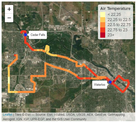
Figure 1.
Map of the Waterloo–Cedar Falls air temperatures. The temperature is measured in degrees Celsius.
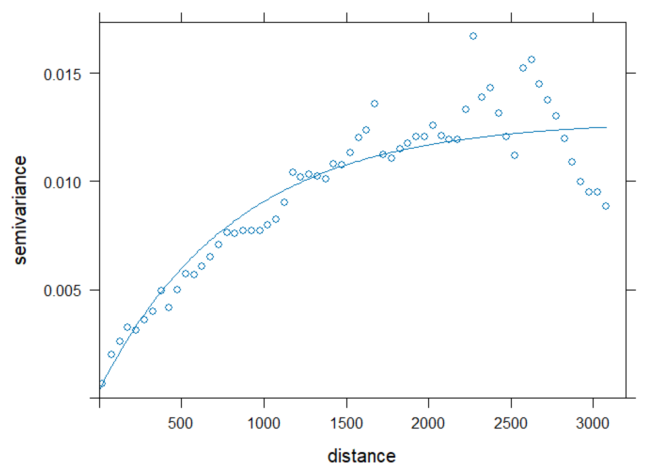
A geostatistical model [28,29] provides a different way, compared to a trend surface model, to incorporate the X-Y locations into a spatial model. Geostatistical models explain any spatial correlation present in the region. Spatial correlation means that two air temperatures observed closer in geographic space are much more similar (after adjusting for model covariates) than a pair of air temperatures observed farther apart. An empirical variogram, seen in Figure 2, constructed from the OLS regression residuals, provides evidence of spatial correlation [30]. Note that an exponential theoretical variogram was fitted to the empirical variogram in Figure 2 for illustrative purposes only. A geostatistical spatial linear model fits the exponential correlation structure, simultaneous with the landscape variables. Figure 2 is a diagnostic tool that illustrates the need to model spatial correlation using a geostatistical model. Therefore, an exponential correlation function was fitted, simultaneously with the twenty landscape variables in a geostatistical model, to the nighttime WCF air temperature data [31], resulting in a spatial correlation of 3452.7 m, or a little over two miles.
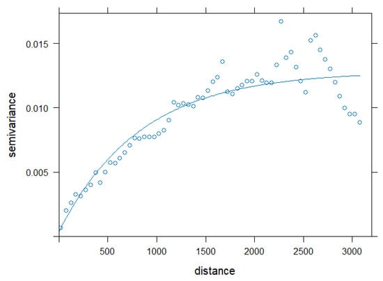
Figure 2.
Theoretical Exponential Variogram fitted to the Empirical Variogram produced from the OLS Multiple Regression residuals. Note that X = Lag distance is measured in meters.
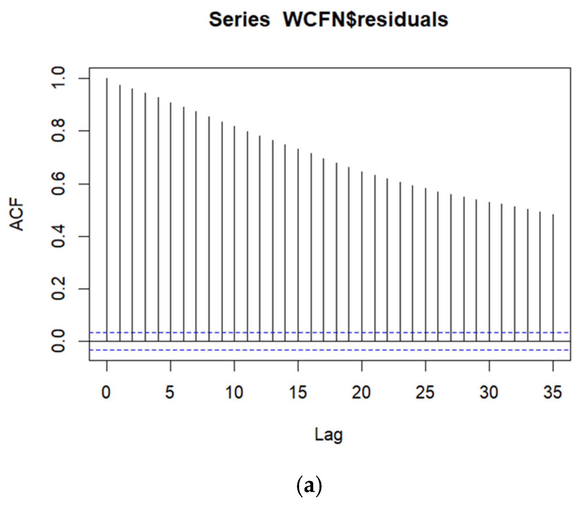
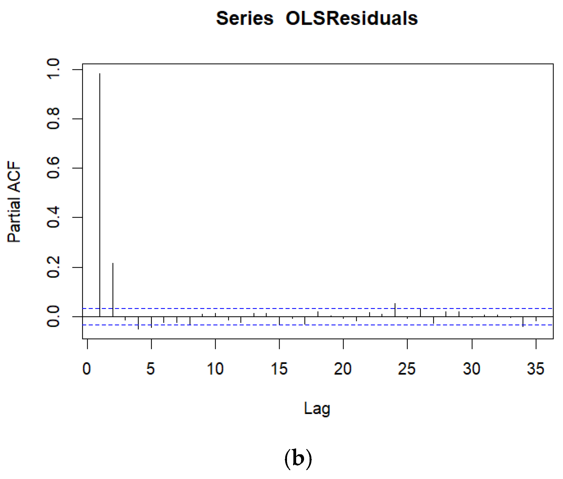
A time series model ([22], Chapter 12) was fitted because both the autocorrelation function (ACF) and partial autocorrelation function (PACF) plots of the OLS regression residuals indicate temporally correlated data, as seen in Figure 3a and Figure 3b, respectively. Temporally correlated data mean that two observations closer in time are much more similar (after adjusting for covariates) than two observations further apart in time. Therefore, an autoregressive integrated moving average (ARIMA) time series model [32] was fitted to the WCF nighttime air temperatures, whereby an ARIMA(p = 1, d = 1, q = 3) model provided temporally uncorrelated residuals. It is not surprising that a differencing component (d = 1) is needed in the ARIMA model, given the presence of long-range correlation, as seen in the slow decay of the autocorrelation in the ACF plot of the OLS regression residuals in Figure 3a. The ARIMA time series best-fitting model adds five extra parameters (an autoregressive term and three moving average parameters for sequentially differenced data) over and above the OLS regression model.
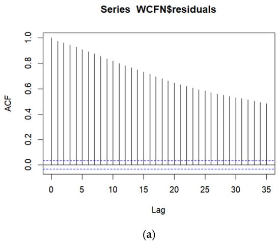
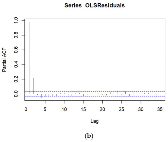
Figure 3.
(a). Autocorrelation Function Plot for the residuals from the OLS Multiple Regression. Note that X = Lag is measured in time and the dashed horizontal lines represent confidence intervals. All lags in the ACF plot are statistically significantly different from zero. (b). Partial Autocorrelation Function Plot for the residuals from the OLS Multiple Regression. Note that X = Lag is measured in time and the dashed horizontal lines represent confidence intervals. The first two lags in the PACF plot are statistically significantly different from zero.
Next a random forest (RF) model was fitted to the WCF nighttime air temperature data. However, we note that, while model averaging statistical techniques (e.g., random forests and Bayesian hierarchical models) will typically explain air temperatures better [18], concerns of overfitting the existing dataset, generalization of the results to other data, choice and tuning of the hyperparameters, and lack of explanatory transparency are potential downsides. The Results section of this paper will empirically demonstrate the utility and limitations of RF modeling.
2.3. Predicting WCF Air Temperatures
An analysis of the WCF nighttime air temperature dataset helps to address the question of what a useful strategy might be to predict a target city’s air temperatures when no data have been collected in that city. Given our objective of using a substitute city’s data to potentially predict air temperature in another city, we use only the original twenty landscape variables (i.e., mean and standard deviation of NDVI, CC, CDM, BH, BV) at 100 and 800 m neighborhood distances, because any temporal or spatial component of the substitute city’s fitted model would not be appropriate for the target city. In other words, the trend surface, time series, geostatistical, and random forest models are not used going forward.
Specifically, by employing the twenty landscape variables, we examine how well the WCF air temperatures (afternoon, evening, and nighttime) are predicted (a) using only data from WCF, but collected at a different time of the day, (b) by data from each individual (non-WCF) substitute city, and (c) after pooling data across all cities (omitting WCF data at any time period). Although the findings presented in the Results section, below, will indicate that using data collected at a different time of day (but from the same city) provides superior prediction of air temperatures in that city, doing so is not possible when no measurements, at any time of day, have been collected for a given urban area. Section 2.4 provides a rationale for examining “substitute-city” strategies for predicting air temperatures in unsampled urban areas.
2.4. Substitute-City Cross-Validation Strategies
Any cross-validation technique requires a training, calibration, or validation dataset consisting of data used as inputs to the model. That is, the statistical model or fitting algorithm is fine-tuned, evaluated, or formed using the training dataset (e.g., the OLS regression model supplies parameter estimates, which can then be used for prediction). To illustrate with an example, one can pool all nighttime data across all Iowa cites (except WCF) to predict the 3,623 nighttime air temperatures recorded only in WCF. Therefore, the pooled nighttime data (except for data from WCF) serve as the training dataset.
The testing, target, or holdout dataset will not be used to fit the model but contains the actual ground-truth air temperatures at locations for which predicted values can be tested. The model is fitted to the training dataset and then predicts air temperatures at locations in the external testing dataset. The testing dataset will have model-based predictions, together with the corresponding true air temperatures, which allow an assessment of model accuracy.
Most generally, formation of the testing dataset follows one of two approaches, where the first approach consists of external prediction of a holdout set of completely new-to-the-model observations that were never employed, at any point, in the model’s construction Note that OLS regression models have the same training and testing datasets, hence providing internal model prediction. In contrast, external prediction conveys that the target dataset is not used by the model except when providing prediction. Kutner, Nachtsheim, and Neter ([22], p. 370) state that “[t]he best means of model validation is through the collection of new data”. For the example in the first paragraph, the dataset of 3623 nighttime air temperatures from WCF serves as the new-to-the-model, external testing dataset.
In contrast, a second common CV approach derives external prediction for the one-and-only-one dataset used in the analysis [33]. That is, the concurrent data can be cross-validated by cycling through the data, withholding a single observation, and then predicting that left-out observation by, for example, performing leave-one-out cross-validation (LOOCV) or walk-forward cross-validation [30]. Each original observation would then have its own left-out prediction to compare to its actual air temperature. One could, alternatively, partition the original dataset into, say, a 70/30 split ([22], Section 9.6) where 70 percent of the data are used to train or fit the model while 30 percent are used to assess prediction. The second CV approach would be appropriate if one only has, say, the 3623 WCF nighttime air temperatures dataset. In this case, one could perform LOOCV or partition the 3623 values into a 70/30 training/testing dataset split, whereby 2536 (70%) data values are used to train or fit the model (for example, running an OLS regression using the 2536 input data values) and 1087 (30%) observations assess the model’s prediction. One potential downside of a 70/30 split is that 1087 WCF nighttime air temperatures (30 percent of the data) are lost as inputs to fit the model, while only one observation would be left out under an LOOCV approach.
We adopt the completely new-to-the-model training dataset CV approach in this study, because our main objective is to determine which substitute Iowa city’s input dataset best predicts another city’s air temperatures. Regardless of any training/testing dataset CV approach, a model choice criterion is needed to decide which city’s air temperatures best predict another city’s air temperatures. Note that many possible model choice criteria, such as sum of squared error (SSE), Akaike information criterion (AIC), R-squared, adjusted R-squared, mean squared (prediction) error, Sawa Bayes information criterion (SBIC), Mallows Cp, Bayes factor, etc., can be used for selecting the “best-fitting” model. See Section 9.3 of Kutner, Nachtsheim, and Kutner [22] and Section 13.2 of Ott and Longnecker [34]. In this study, we choose the predictive R-squared, which is defined as the squared correlation between the cross-validated air temperatures and their corresponding actual air temperatures. Note that an alternative definition of the predictive R-squared is 1- PRESS/SSTotal, where the predicted residual sum of squares error (PRESS) is defined under an LOOCV strategy ([22], p. 360) as PRESS = where is the fitted value omitting the ith observation. Also, sum of squared total = SSTotal = (n − 1) ∗ , which is the numerator of the sample variance of the dependent variable, y. This alternative predictive R-squared definition mimics the usual R-squared definition (as R-squared = 1 − SSE/SSTotal; see Ott and Longnecker, [34], Section 13.2) and is most appropriate for the second CV strategy. Note that predictive R-squared values can be negative (for poorly fitting models) since the PRESS value can be larger than SSTotal, while, in contrast, the usual regression SSE must be less than or equal to SSTotal. The predictive R-squared value reflects how well the model output (forecasted air temperatures) for any one city matches the actual air temperatures in the target city. The interpretation of the predictive R-squared is (nearly) identical to that when using a standard regression R-squared [22], as the percent of (predictive) variability explained by the model.
We develop four CV strategies or procedures for choosing which individual Iowa training city, according to the selected strategy, best forecasts the target city’s air temperatures. If one substitute-city strategy performs best, then that provides one piece of evidence that this best-performing procedure may be generally applicable to cities not sampled in this study. The four substitute-city CV strategies or procedures that are evaluated for their efficacy are:
- Temporal Comparability Strategy: The Date or Closest in Time CV procedure will use the most closely sampled city in time (whose data are antecedent) to predict the target city’s air temperatures.
- Closest Geographic City Strategy: The Closest City or Geography CV procedure will use the geographically closest city to predict the target city’s air temperatures.
- City Size Strategy: The City Size or Population CV procedure will use the city with the most similar, but lower, population to predict the target city’s air temperatures.
- Human Footprint Strategy: The Human Footprint or Cluster Analysis CV procedure will use the city whose landscape variables are determined to be most similar by the dendrogram from an agglomerative hierarchical cluster analysis. The dendrogram was developed using the twenty explanatory landscape variables, which consist of the means and standard deviations for the BH, BV, CC, CDM, and NDVI variables. Figure 4 demonstrates a dendrogram derived for the nighttime air temperatures in WCF. Note that there is a separate dendrogram for each time of day (afternoon, evening, and nighttime), since different X-Y locations were sampled in each city at these different times.
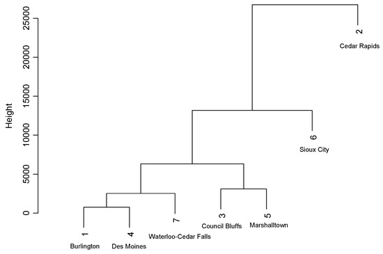 Figure 4. Cluster analysis dendrogram for nighttime data prediction employing the twenty landscape variables.
The four CV strategies are performed for each of the nine urban areas (10 total cities) and three times of air temperature monitoring. Exceptions are if a given city/time did not have a set of measured data (e.g., in Marshalltown, no evening data were collected due to weather conditions, see Coproski et al. [6]) or for strategy 1 where the earliest sampled city (Waverly, sampled on 14 June 2022, as seen in Table 1) has no earlier substitute-city dataset or for strategy 3 where the smallest city (Waverly) has no smaller city to use.
3. Results
This section reports results in subsections corresponding to the three main objectives presented at the very beginning of Section 2 (Materials and Methods). Specifically, Section 3.1 provides further detail regarding data collection, while Section 3.2 discusses the statistical modeling of the nighttime WCF air temperatures in support of Objective 1 (as seen at the very beginning of the Materials and Methods section). Furthermore, Section 3.3 provides details that support the conclusion that air temperatures for the target city of WCF, collected at a different time of day, best predict WCF’s air temperatures, in support of Objective 2. Lastly, the substitute-city CV results are presented in Section 3.4. They are broken down by time of day (nighttime air temperatures in Section 3.4.1, evening in Section 3.4.2, and afternoon in Section 3.4.3) in support of Objective 3.
3.1. Study Area, Temperature Measurements, and Landscape Variables
A thorough explanation regarding how the temperature measurements were actively collected can be found in Coproski et al. [6]. To summarize, a minimum of 3623 (WCF) and a maximum of 29,817 (Des Moines) temperature measurements were recorded during three separate time periods (afternoon, evening, and nighttime) for as many as nine Iowa urban areas (Waterloo–Cedar Falls are bordering, sister cities). Figure 5 shows the Iowa urban areas where air temperature data were collected. Exceptions to the 3× time collection (afternoon, evening and nighttime) are attributed to equipment issues or inclement weather (thunderstorm) that caused nighttime measurements to be missed in Waverly and Fort Dodge and evening measurements being skipped in Marshalltown.
Figure 5.
The nine urban areas in Iowa (10 total cities, but note that Waterloo and Cedar Falls are adjacent, sister cities that were sampled together) where sampling was performed in 2022. See Coproski et al. [6].
The twenty independent landscape variables (the mean and standard deviation for NDVI, CC, CDM, BH, BV) at both 100 and 800 m neighborhood distances were calculated as raster surfaces. Subsequently, the value for each of these landscape variables was calculated by centering concentric circles (of radii of 100 and 800 m) on the location of each air temperature measurement. Thus, an overall table was created holding the measured air temperature, time and date, and x and y locations, together with each of the twenty landscape variables for all sampled locations in each city.
3.2. Results of the Statistical Modeling Techniques for One Urban Area (Waterloo–Cedar Falls)
The results from the statistical models for WCF nighttime air temperatures are presented in Table 2a–c. As seen in the second column of Table 2a, all landscape variable means in the OLS regression are very strongly statistically significant (p-value < 0.01) in explaining nighttime air temperatures in WCF. Moreover, many variables are of the expected sign, meaning that, for example, a higher percentage of canopy cover or a higher NDVI value is associated with reduced air temperature. As seen in the second column of Table 2b, the variability associated with the independent variables in 100 and 800 m concentric circles is less clear, as only seven of the ten variables are very strongly statistically significant. To illustrate, more variability in canopy cover or NDVI (in a circle with a radius of 800 m around each sampled air temperature) is associated with higher air temperature. In total, the OLS regression model explains 71.5 percent of the variability in nighttime WCF air temperature, as seen in Table 2c.
Table 2.
(a) Statistical model results for landscape variable mean values for WCF nighttime air temperatures. (b) Statistical model results for landscape variable standard deviation values for WCF nighttime air temperatures. (c) Model diagnostics for WCF nighttime air temperatures (n = 3623).
As seen in the third column of Table 2a and Table 2b, respectively, many of the same landscape variables that were statistically significant in the OLS regression model are also statistically significant for the second order trend surface model. Furthermore, all five trend surface parameter estimates were very strongly statistically significant (p-value < 0.01). This result helps to explain why using data from the same city (even when collected at a different time of day) will better predict air temperatures compared to using data from a different urban area.
The geostatistical model indicates that the spatial correlation is very strong for the WCF nighttime air temperatures and, as a result, mostly washes out the fixed effect landscape variables (that were observed as very strongly statistically significant in both the OLS and trend surface regressions). As seen in the fourth column of Table 2c, the lower predictive R-squared and higher sum of squared error (SSE) values for the geostatistical model, respectively, indicate that both the OLS and trend surface regression models fit better than the geostatistical model.
As noted in the Materials and Methods section, the ARIMA model adds five extra parameters (an autoregressive term and three moving average parameters for sequentially differenced data) over and above the OLS regression model. These additions provide marked improvement in explanation, as seen in the fifth column of Table 2c. The SSE and Akaike information criterion (AIC) values were lowest ([22], Section 9.3) for the time series model and the predictive R-squared value was highest when compared to the previous three models. In addition, the parameter estimates, as seen in the last column in Table 2a ,b, are fairly consistent with that seen from the OLS regression.
Next, a random forest (RF) model was fitted to the WCF nighttime air temperature data, resulting in an R-squared value of 0.9901 with an SSE of 1.133 as seen in Table 2c. Of the five models fitted, the RF model best explained the existing nighttime WCF air temperatures. However, we note that, while model averaging statistical techniques (e.g., random forests and Bayesian hierarchical models) will often predict air temperatures better [18], concerns of overfitting the existing dataset, generalization of the results to other data, choice and tuning of the hyperparameters, and lack of explanatory transparency are potential downsides.
In examining the commonalities for the coefficients, as seen in Table 2a,b, for the first four fitted models (a random forest model, by design, does not provide parameter estimates for the individual landscape variables), the NDVI means in Table 2a are strongly significant for all models (at either the 100 or 800 m scale or both) in explaining air temperature. More vegetation, resulting in a higher NDVI, is associated with lower air temperatures. While all of the mean variables are statistically significant for the OLS regression, as seen in the second column of Table 2a, the trend surface model has nine statistically significant variables (but also incorporates five statistically significant trend surface variables); the time series loses four (but incorporates five extra parameters for the ARIMA(1,1,3) model) and the geostatistics model loses all but two (but incorporates the range, sill, and nugget components of the spatial correlation-variogram model).
Looking at the model summaries for all five models in Table 2c, the geostatistical model performed worst, while the RF model, not surprisingly, best explained the existing nighttime air temperatures in WCF, given its use of (the default) 500 trees in its fitting algorithm. Interestingly, the time series model fit nearly as well as the RF model, but the time series model allows for parameter estimates, as seen in the last column of Table 2a,b, which, apparently, should not be a surprise, given the strong temporal correlation of the collected air temperature data (as seen in Figure 3a).
While a thorough analysis of WCF nighttime air temperatures is of importance, the larger question of how to best predict a target city’s air temperature, when not using any directly collected data in the target city, is a main focus of this research. Given our objective of using a substitute city’s data to predict air temperatures in another city, we only use the twenty landscape variables in the subsequent sections, because any temporal or spatial component of the substitute city’s fitted model would not be appropriate for the target city. In other words, we are eschewing the trend surface, geostatistical, time series and RF models going forward.
3.3. Results When Predicting WCF Air Temperatures
Employing the twenty landscape variables, we examine how well the WCF air temperatures, collected in the afternoon, evening, and nighttime, are predicted: (a) using only data from WCF, but collected at a different time of day, (b) by data from each individual (non-WCF) city, and (c) after pooling data across all cities (omitting any WCF data collected at any time of day).
When predicting nighttime air temperatures in WCF, the best predicting input dataset came from using afternoon data from WCF (predictive R-squared = 0.4494), as seen in Table 3a. The evening WCF air temperature data gave the second highest predictive R-squared value (0.4069). The best predicting individual Iowa city (apart from WCF data collected at a different time of day) was Des Moines (0.3932), while the worst predicting city was Marshalltown (0.0066). Pooling the data across all cities (except for the WCF data collected at any time of day) ranked seventh (0.1223).
Table 3.
(a) Prediction of Waterloo–Cedar Falls air temperature—nighttime. Note that Two Iowa cities (Fort Dodge and Waverly) were not sampled at nighttime. (b) Prediction of Waterloo–Cedar Falls air temperature—evening. (c) Prediction of Waterloo–Cedar Falls air temperature—afternoon.
Similar results can be seen in Table 3b, when predicting evening WCF air temperatures. Afternoon WCF air temperatures best predicted evening temperatures (predictive R-squared = 0.4956), while the nighttime WCF air temperature data only forecast fourth best (0.3902). The best predicting individual Iowa city (apart from WCF data collected in the afternoon) was Cedar Rapids (0.4103). Interestingly, Des Moines predicted worst (0.1238) for evening WCF air temperatures. Like the results for the nighttime WCF data, pooling all of the non-WCF data predicted only seventh best (0.2441).
The results for predicting afternoon WCF air temperature can be seen in Table 3c, where WCF evening data only were third best (predictive R-squared = 0.4507). The best predicting individual Iowa city was Des Moines (0.4921), while the worst predicting city was Waverly (0.0019). The evening WCF data performed third (0.4507), while pooling all data (except for data from WCF) was eighth (0.2198).
As seen in Table 3a–c, predicting WCF air temperature, especially during the evening or nighttime, is best performed using data collected from WCF at a different time of day. Pooling data performs poorly when predicting WCF data at any time of the day, with its highest predictive R-squared of 0.2441. In addition, an analysis of covariance (ANCOVA) F-test ([34], Chapter 16) indicates that any statistical analysis needs to be performed by city (F = 37.57, p-value = 0) rather than pooling data.
In summary, the analysis in this section reinforces the observation that data from the same city, when collected at a different time of day, best forecast that city’s air temperature. It also shows that one city does not universally best predict WCF air temperature at various times of the day, as Des Moines is the individual Iowa city that best predicted both WCF nighttime and afternoon data but performed worst in predicting evening air temperatures.
3.4. Substitute-City Cross-Validation Results for All Sampled Iowa Cities
As discussed in Section 2.4, four CV strategies are evaluated when predicting air temperatures in an unsampled urban area. Each CV strategy predicts air temperatures in the target city using the input air temperature OLS regression results from the selected city according to the following criteria: (1) choose the most closely sampled city in time (closest, but antecedent sampling date), (2) pick the closest city based on geography or location, (3) select the city that is closest in size, but with a lower population, and finally (4) choose the city whose landscape variables, based on the cluster analysis of the twenty independent variables, most closely resemble those of the target city.
The results for the four substitute-city CV strategies for nighttime data for seven Iowa urban areas are detailed in Table 4, Table 5, Table 6 and Table 7 and detailed in the first subsection. In the second subsection, we discuss the substitute-city CV results by city for all three times of day, while the third subsection focuses on the overall results for each CV strategy by time of day.
Table 4.
Prediction results for nighttime air temperatures—Closest in Time CV strategy.
Table 5.
Prediction results for nighttime air temperatures—Closest City CV strategy. Notes: WCF = Waterloo Cedar Falls and the parenthetic Predictive R-squared in the last column is the “Predicted by” city’s percent of variability explained by the model.
Table 6.
Prediction results for nighttime air temperatures—City Size or Population CV strategy. Notes: WCF = Waterloo–Cedar Falls and the parenthetic Predictive R-squared in the last column is the “Predicted by” city’s percent of variability explained by the model.
Table 7.
Prediction results for nighttime air temperatures—Cluster Analysis or Human Footprint CV strategy. Notes: WCF = Waterloo–Cedar Falls and the parenthetic Predictive R-squared in the last column is the “Predicted by” city’s percent of variability explained by the model.
3.4.1. Substitute-City Cross-Validation Results for Nighttime Data
The results for the Date or Closest in Time CV procedure are presented for nighttime data in Table 4 where, for example, WCF nighttime data were collected between 4 and 5 a.m. on 22 September 2022. According to the Date procedure, WCF air temperatures are best predicted by the substitute-city of Council Bluffs (since Council Bluffs data were collected on August 14, as seen in Table 1). However, as discussed previously, and as seen in Table 3a and Table 4, Des Moines is the substitute Iowa city that best forecasts WCF nighttime air temperatures (predictive R-squared = 0.3932). Council Bluffs (predictive R-squared = 0.1683, as seen in parentheses in the Predictive R-Squared column of Table 4) is the fourth best predicting substitute city for WCF nighttime data (as seen in the Rank column in Table 4). Examining Table 4, the Date procedure did not provide a best predicting training dataset for any of the individual Iowa cities; its best performance was second in predicting both Marshalltown’s (0.5543) and Council Bluff’s (0.2941) nighttime air temperatures.
The results for the Closest City or Geography CV procedure are presented for nighttime data in Table 5, where, for example, Cedar Rapids would be expected to best predict WCF nighttime air temperatures (as seen in the second column of Table 5), since Cedar Rapids is the closest sampled city to WCF. However, Cedar Rapids, as the input city for WCF, has a quite low predictive R-squared (0.0347, shown in parentheses in the last column of Table 5) and ranked fifth out of the seven individual Iowa cities when predicting WCF nighttime air temperatures. Overall, the Closest City CV strategy best predicted air temperatures in only two cities: Sioux City (0.2158) and Cedar Rapids (0.1999), as seen in the Rank column of Table 5.
The results for the Population CV procedure are presented for nighttime data in Table 6, where, for example, Sioux City should provide the training dataset for WCF nighttime air temperatures, since Sioux City has a population of 85,727 compared to 107,343 for WCF. As seen in Table 6, Sioux City was the second best at predicting WCF temperatures (predictive R-squared = 0.2520). Moreover, the Population procedure best predicted each of the other five cities’ air temperatures, as seen in the Rank column of Table 6, with the highest predictive R-squared value being 0.5874.
The Human Footprint CV procedure chooses a training dataset city that best matched the landscape variables of the target city, via the dendrogram from an agglomerative hierarchical cluster analysis [35]. A similarity metric (e.g., Euclidean, Mahalanobis, or Manhattan distance) first compares all possible () pairs of multivariate observations to determine which pair of cities has the most similar collection of landscape variables.
Examining the dendrogram in Figure 4, Des Moines and Burlington have the most similar set of landscape variables, since they are joined first at the bottom of the dendrogram. Therefore, the Human Footprint procedure would suggest that Des Moines and Burlington would be the other city’s respective training dataset for predicting nighttime air temperatures, as seen in the second column of Table 7. Waterloo–Cedar Falls is next added to the dendrogram, as its landscape variables are most similar to the first formed cluster, consisting of Des Moines and Burlington (after employing an average linkage method to judge how similar WCF is to the merged Des Moines and Burlington cluster). Therefore, either Des Moines or Burlington is suggested to predict WCF nighttime air temperatures. The Human Footprint CV strategy chooses to use the city that is closer in population, whenever there is a choice between two just-merged-in-the-dendrogram cities. To further illustrate, as seen in Figure 4, Sioux City (population 85,727) would have, according to the Human Footprint strategy, Council Bluffs (62,399), rather than Marshalltown (27,574), as its training dataset city when predicting nighttime air temperatures.
Dendrograms from the landscape variables computed during the afternoon and evening will potentially produce a different training dataset city for each target city. That is, unlike the other three substitute-city CV strategies, the Human Footprint procedure depends upon the landscape variables computed at the sampled locations. For example, Burlington is best predicted by WCF from the afternoon and evening landscape variable dendrogram, but Burlington uses Des Moines when predicting nighttime air temperatures (as seen in Table 7). In contrast, the Closest City procedure will always choose Cedar Rapids to predict Burlington’s air temperatures, as seen in Table 5, regardless of the time of day when prediction is desired.
As seen in Table 7, nighttime air temperatures in WCF are best predicted by Des Moines (predictive R-squared = 0.3932), which is also the input city according to the Human Footprint strategy. Looking at the Rank column in Table 7, two other cities, Council Bluffs and Sioux City, also had the Cluster Analysis procedure accurately pick their training dataset (predictive R-squared values of 0.5874 and 0.2158, respectively). However, the best that the Human Footprint procedure performed for the remaining cities was fourth. The Cluster Analysis strategy either performed very well or poorly, with no middle ground.
3.4.2. Cross-Validation Results by City for Afternoon, Evening, and Nighttime Data
Details regarding how well the four substitute-city CV procedures performed for each city can be seen in Table 8a–c for the afternoon, evening, and nighttime air temperatures, respectively. Inspecting the nighttime air temperature results in the Rank column of Table 8a, all cities except Burlington had at least one strategy accurately provide the best predicting input city. Furthermore, Sioux City had three CV strategies that suggested using Council Bluffs as the substitute-city training dataset: Geography as seen in Table 5, Population in Table 6, and Human Footprint in Table 7 (only the Date procedure suggested a different input city—Marshalltown—as seen in Table 4). Because nighttime air temperatures in Sioux City were best predicted using the substitute city of Council Bluffs (predictive R-squared = 0.2158), the three substitute-city CV strategies (Geography, Population, and Human Footprint) each accurately forecasted the best predicting substitute city.
Table 8.
(a) Best predicting CV strategy by city—nighttime temperatures. (b) Best predicting CV strategy by city—evening temperatures. (c) Best predicting CV strategy by city—afternoon temperatures.
The Population procedure accurately predicted a total of five cities’ (Cedar Rapids, Council Bluffs, Des Moines, Marshalltown, and Sioux City) nighttime air temperatures as seen in second column of Table 8a. The Closest City and Cluster Analysis procedures best predict three cities (Burlington, Cedar Rapids, and Sioux City for the Geography procedure; Council Bluffs, Sioux City, and WCF for the Human Footprint procedure), while the Date procedure forecasted no best fitting input cities.
For evening air temperatures, only two cities had their input city correctly forecasted, Council Bluffs and Des Moines as seen in the Rank (of 1) column in Table 8b. The Population procedure not only accurately picked these two cities’ training datasets but also finished second best for three other cities (Cedar Rapids, Fort Dodge, and WCF). That is, for five of the eight cities in which evening air temperature data were collected, the Population procedure forecasted best (technically, the Population procedure was at least as good or better than any other strategy for five of the eight cities). The Geography and Cluster Analysis procedures each best predicted two cites (Burlington and Cedar Rapids for Geography, Council Bluffs and Waverly for Cluster Analysis), while the Date procedure had only one (Sioux City).
For afternoon air temperatures, five cities had their input city correctly forecasted, Burlington, Cedar Rapids, Marshalltown, WCF, and Waverly, as seen in the Rank (of 1) column in Table 8c. The Cluster Analysis procedure performed best when predicting input datasets in four cities (Cedar Rapids, Council Bluffs, Sioux City, and WCF). The Date procedure best forecasted three (Burlington, Fort Dodge, and Marshalltown); the Population procedure had two (Council Bluffs and Des Moines) and the Geography procedure had just one (Waverly).
3.4.3. Cross-Validation Overall Strategy Results for Afternoon, Evening, and Nighttime Data
Looking back at Table 6, the Population substitute-city CV best predicted five of the six cities for which nighttime data were collected. Inspecting Table 9a, the average rank for the Population procedure was 1.17 (averaging the Rank column in Table 6, except for Burlington). The next best performing CV strategy, the Closest City or Geography procedure, averaged 3.14 (by averaging the Rank column in Table 5). It is quite surprising that the Population procedure performed so well for nighttime data, with all six cites producing a Population procedure rank of either first or second (hence the “6” entry in the “Number of Top Three” column of Table 9a).
Table 9.
(a) Strategy or procedure prediction results—nighttime prediction summary. (b) Strategy or procedure prediction results—evening prediction summary. (c) Strategy or procedure prediction results—afternoon prediction summary.
Looking at evening air temperature results in Table 9b, the Population procedure also performed best with an average rank of 2.43 and five of the six cities being predicted under the Population procedure were ranked in the top three, as seen in the third column of Table 9b. As seen in Table 9c, none of the four strategies distinguished themselves when forecasting afternoon air temperatures, with, technically, the Population procedure being tied for best with the Geography procedure, with each having an average rank of 4. However, as discussed previously, the Human Footprint and Date procedures best predicted afternoon air temperatures in the most cities (four for Cluster Analysis and three for Date). Overall, better predictive ability occurs during the evening and at night, attesting to the observation that the greatest variation in air temperature occurs overnight [7].
The Population substitute-city CV strategy provided surprisingly strong results for the nighttime data, solid results for the evening data, and poor results for the afternoon data. We say surprising because it was thought, a priori, that picking the substitute city with the best matching landscape variables (to the target city) would provide quality prediction. That is, we fully expected the Human Footprint procedure to forecast best. Instead, matching the city size (via the Population substitute-city CV strategy) provides the best predictive power.
Wei et al. [5] quantified the relationship between population size and UHIs in a meta-analysis of over 150 studies. They concluded that larger cities are associated with higher temperatures because the increased density of buildings corresponds to higher amounts of human activity, with more emission of heat and pollution. Wei et al. [5] also concluded that, because so few published papers have offered a quantitative analysis of UHIs, “more studies are needed, across a wider set of cities, and using more of similarly defined observed measurements” to better understand the relationship between air temperature and population size. Therefore, our study empirically reinforces the findings in Wei et al. [5], in that similar sized cities should be expected to have similar temperature profiles, especially at nighttime, when the urban area has the opportunity to cool.
4. Conclusions
No substitute city will provide perfectly accurate prediction of air temperature for any one unsampled city, at any one X-Y location, and at any one time of day; there is simply too much variability in air temperatures within and across cities. However, the CV results indicate that using the city closest in population to the target city will produce relatively reliable predictions. That is, the air temperature data from the substitute city, according to the Population procedure, will best provide predictions that are in concordance with actual air temperatures; where temperatures are high the model accurately predicts high temperatures and, where temperatures are low, the model will well-predict low temperatures. Note that accurate mapping of temperature contours results from choosing the (squared) correlation between the set of actual and predicted air temperatures (the predictive R-squared model choice criterion) to judge the best fitting model, instead of using a squared difference, such as the AIC or mean squared (prediction) error.
Although not reported here, the authors have expanded the development of the five landscape variables based on LiDAR and aerial imagery data to all cities in Iowa that have a population of more than 10,000 inhabitants (~40 cities). The intention is to apply the relevant substitute city model (closest in population, but smaller) to those cities. There were several Iowa cities (Ottumwa, Independence, Davenport) where air temperatures were collected in 2023 that could be subsequently used to further test the predictive strategy described here (Population procedure). As was mentioned previously, there seems to be little research in attempting to apply this type of predictive strategy for providing relative temperature surfaces or maps in unsampled urban areas.
In this work, we collect and analyze air temperature data from as many as nine urban areas (ten total cities) in Iowa at three times of the day (afternoon, evening, and nighttime). Landscape variables: building height, building volume, canopy cover, canopy density metric, and NDVI, are calculated at 100 and 800 m radii around each sampled air temperature location. Five statistical models, an OLS regression, trend surface, geostatistical, time series, and random forest model, are then fitted using the landscape variables as covariates. A random forest model best explains the existing air temperature data, while a time series model explains almost as well as the random forest model but allows for interpretation of its model parameters.
The primary objective of this paper was to develop and examine forecasting strategies when concurrent data from a target city (where air temperature maps are desired) are unavailable. We empirically show that using data from a different time of day will best predict the target city’s air temperatures, using WCF nighttime air temperatures. We also show that pooling all non-WCF data provides poor prediction. Therefore, we explore the tenability of using a substitute city when forecasting the unsampled target city’s air temperatures.
We develop four CV strategies that each pick a substitute city for predicting near-surface air temperatures in the unsampled target city. These four CV strategies are: choose the substitute city that is (a) closest geographically, (b) closest in population, (c) sampled closest in time, and (d) has the most similar human footprint of landscape variables, established via a dendrogram from an agglomerative hierarchical cluster analysis. Analysis of these four substitute-city CV strategies for the nine Iowa urban areas (ten total cities) indicates that the Population CV procedure forecasts nighttime and evening air temperature surprisingly well, while no substitute-city CV strategy outshined the others when forecasting afternoon air temperature.
Author Contributions
Conceptualization of the study: J.P.D., J.T.D., B.L., C.A.C. (original temperature collection and modeling are reported in Corposki et al. [6]). M.D.E. was primarily responsible for developing the cross-validation strategies. Methodology: Each author contributed to the development of the study methodology. Software: J.T.D. developed sensor Python (version 3.1.1) scripts and post-processing temperature data Python scripts while C.A.C., with assistance from J.P.D. and J.D., was primarily responsible for the development of automated GIS processing (Python, arcpy) scripts, and M.D.E. was responsible for all statistical modeling/code using RStudio (Version 12.1+563) and/or S-Plus (Version 8.2 for Windows). Writing, reviewing, and editing were carried out by all authors, with the original draft developed by M.D.E. and J.P.D. Project administration: J.P.D. was the primary project lead. Funding acquisition: J.P.D., with assistance from J.T.D. and B.L., wrote the proposal that led to the funding of this study. All authors have read and agreed to the published version of the manuscript.
Funding
This research was funded by the Iowa Economic Development Authority Iowa Energy Center Grant Program (agreement number 21-IEC-012).
Institutional Review Board Statement
Not applicable.
Informed Consent Statement
Not applicable.
Data Availability Statement
The 2022 air temperature monitoring data and independent landscape variables (as raster spatial datasets) can be found at https://www.geotree.uni.edu/web/IowaUrbanHeatProject_IowaEnergyCenter/IowaUrbanHeat_MonitoringModeling.zip (accessed on 23 April 2025). Three Excel files were created for afternoon, evening, and nighttime data. Each contains the air temperature measurements, time and date, and x and y locations, together with the twenty landscape variables for all sampled locations in the nine urban areas (10 cities). These data plus the 3623 WCF nighttime air temperature measurements together with the R code and results for the WCF nighttime statistical models can be found at https://www.geotree.uni.edu/web/IowaUrbanHeatProject_IowaEnergyCenter/RawTemperatureData_IndependentVariables_StatisticalModeling.zip (accessed on 23 April 2025).
Acknowledgments
Several University of Northern Iowa Geography students assisted in air temperature data collection, including Lindsey Hubbell and Casey Shanaberger.
Conflicts of Interest
The authors declare no conflicts of interest. The funders had no role in the design of the study; in the collection, analyses, or interpretation of data; in the writing of the manuscript; or in the decision to publish the results.
Abbreviations
The following abbreviations are used in this manuscript:
| ACF | Autocorrelation Function |
| AIC | Akaike Information Criterion |
| ANCOVA | Analysis of Covariance |
| ARIMA | Autoregressive Integrated Moving Average |
| BH | Building Height |
| BV | Building Volume |
| CART | Classification and Regression Tree |
| CC | Canopy Cover |
| CDM | Canopy Density Metric |
| CV | Cross-Validation |
| EPA | Environmental Protection Agency |
| GIS | Geographic Information System |
| LiDAR | Light Detection and Ranging |
| LOOCV | Leave-One-Out Cross-Validation |
| LST | Land Surface Temperature |
| LULC | Land Use/Land Cover |
| MODIS | Moderate Resolution Imaging Spectroradiometer |
| NDVI | Normalized Difference Vegetation Index |
| OLS | Ordinary Least Squares |
| PACF | Partial Autocorrelation Function |
| PRESS | Predicted Residual Sum of Squares |
| RF | Random Forest |
| SSE | Sum of Squared Error |
| TSM | Trend Surface Model |
| UHI | Urban Heat Island |
| USA | United States of America |
| WCF | Waterloo–Cedar Falls |
References
- Watts, N.; Amann, M.; Arnell, N.; Ayeb-Karlsson, S.; Beagley, J.; Belesova, K.; Boykoff, M.; Byass, P.; Cai, W.; Campbell-Lendrum, D.; et al. The 2020 Report of The Lancet Countdown on Health and Climate Change: Responding to Converging Crises. Lancet 2021, 397, 129–170. [Google Scholar] [CrossRef] [PubMed]
- Hattis, D.; Ogneva-Himmelberger, Y.; Ratick, S. The Spatial Variability of Heat-Related Mortality in Massachusetts. Appl. Geogr. 2012, 33, 45–52. [Google Scholar] [CrossRef]
- Santamouris, M.; Cartalis, C.; Synnefa, A.; Kolokotsa, D. On the Impact of Urban Heat Island and Global Warming on the Power Demand and Electricity Consumption of Buildings—A Review. Energy Build. 2015, 98, 119–124. [Google Scholar] [CrossRef]
- Stone, B.J. Urban and Rural Temperature Trends in Proximity to Large US Cities: 1951–2000. Int. J. Climatol. 2007, 27, 1801–1807. [Google Scholar] [CrossRef]
- Wei, Y.; Lemoy, R.; Caruso, G. The effect of population size on urban heat island and NO2 air polloution: Review and meta-analysis. City Environ. Interact. 2024, 24, 100161. [Google Scholar] [CrossRef]
- Abbeg Coproski, C.; Liang, B.; Dietrich, J.T.; DeGroote, J. Monitoring and Modeling Urban Temperature Patterns in the State of Iowa, USA, Utilizing Mobile Sensors and Geospatial Data. Appl. Sci. 2024, 14, 10576. [Google Scholar] [CrossRef]
- US EPA. What Are Heat Islands? Available online: https://www.epa.gov/heatislands/what-are-heat-islands (accessed on 11 February 2025).
- Oke, T.R. Boundary Layer Climates, 2nd ed.; Methuen: London, UK, 1987; ISBN 978-0-203-40721-9. [Google Scholar]
- Balázs, B.; Unger, J.; Gál, T.; Sümeghy, Z.; Geiger, J.; Szegedi, S. Simulation of the Mean Urban Heat Island Using 2D Surface Parameters: Empirical Modelling, Verification and Extension. Meteorol. Appl. 2009, 16, 275–287. [Google Scholar] [CrossRef]
- Tzavali, A.; Paravantis, J.P.; Mihalakakou, G.; Fotiadi, A.; Stigka, E. Urban Heat Island Intensity: A Literature Review. Fresenius Environ. Bull. 2015, 24, 4537–4554. [Google Scholar]
- Rajasekar, U.; Weng, Q. Urban Heat Island Monitoring and Analysis Using a Non-Parametric Model: A Case Study of Indianapolis. ISPRS J. Photogramm. Remote Sens. 2009, 64, 86–96. [Google Scholar] [CrossRef]
- Bala, R.; Prasad, R.; Yadav, V.P. Quantification of Urban Heat Intensity with Land Use/Land Cover Changes Using Landsat Satellite Data over Urban Landscapes. Theor. Appl. Clim. 2021, 145, 1–12. [Google Scholar] [CrossRef]
- Shiflett, S.A.; Liang, L.L.; Crum, S.M.; Feyisa, G.L.; Wang, J.; Jenerette, G.D. Variation in the Urban Vegetation, Surface Temperature, Air Temperature Nexus. Sci. Total Env. 2017, 579, 495–505. [Google Scholar] [CrossRef] [PubMed]
- Jaber, S.M.; Sengupta, R. Spatial and Temporal Variabilities in Land Surface Temperatures and Near-Surface Air Temperatures in an Arid to Semiarid Urban Region: Implications for Urban Heat Island Research. Geo-Spat. Inf. Sci. 2024, 27, 2137–2161. [Google Scholar] [CrossRef]
- Lu, L.; Weng, Q.; Xiao, D.; Guo, H.; Li, Q.; Hui, W. Spatiotemporal Variation of Surface Urban Heat Islands in Relation to Land Cover Composition and Configuration: A Multi-Scale Case Study of Xi’an, China. Remote Sens. 2020, 12, 2713. [Google Scholar] [CrossRef]
- Shandas, V.; Voelkel, J.; Williams, J.; Hoffman, J. Integrating Satellite and Ground Measurements for Predicting Locations of Extreme Urban Heat. Climate 2019, 7, 5. [Google Scholar] [CrossRef]
- Oukawa, G.Y.; Krecl, P.; Targino, A.C. Fine-Scale Modeling of the Urban Heat Island: A Comparison of Multiple Linear Regression and Random Forest Approaches. Sci. Total Environ. 2022, 815, 152836. [Google Scholar] [CrossRef]
- Voelkel, J.; Shandas, V. Towards Systematic Prediction of Urban Heat Islands: Grounding Measurements, Assessing Modeling Techniques. Climate 2017, 5, 41. [Google Scholar] [CrossRef]
- Molas, A. Can Random Forests Overfit? Medium. 2022. Available online: https://medium.com/@alexmolasmartin/can-random-forests-overfit-a743755251b4 (accessed on 23 April 2025).
- Milà, C.; Ludwig, M.; Pebesma, E.; Tonne, C.; Meyer, H. Random Forests with Spatial Proxies for Environmental Modelling: Opportunities and Pitfalls. Geosci. Model. Dev. 2024, 17, 6007–6033. [Google Scholar] [CrossRef]
- Chen, K.; Newman, A.J.; Huang, M.; Coon, C.; Darrow, L.A.; Strickland, M.J.; Holmes, H.A. Estimating Heat-Related Exposures and Urban Heat Island Impacts: A Case Study for the 2012 Chicago Heatwave. GeoHealth 2022, 6, e2021GH000535. [Google Scholar] [CrossRef]
- Kutner, M.H. Applied Linear Regression Models, 4th ed.; Kutner, M.H., Nachtsheim, C.J., Neter, J., Eds.; McGraw-Hill/Irwin: Boston, MA, USA, 2004; ISBN 978-0-07-238691-2. [Google Scholar]
- Iowa Demographics Iowa Cities by Population. 2025. Available online: https://www.iowa-demographics.com/cities_by_population (accessed on 26 February 2025).
- Bureau, U.C. American Community Survey (ACS). Available online: https://www.census.gov/programs-surveys/acs (accessed on 26 February 2025).
- Ho, H.C.; Knudby, A.; Sirovyak, P.; Xu, Y.; Hodul, M.; Henderson, S.B. Mapping Maximum Urban Air Temperature on Hot Summer Days. Remote Sens. Environ. 2014, 154, 38–45. [Google Scholar] [CrossRef]
- Rossiter, D.G. Trend Surfaces Fitting by Ordinary and Generalized Least Squares and Generalized Additive Models; ISRIC–World Soil Information 2021; Cornell University, Section of Soil & Crop Sciences: Ithaca, NY, USA, 2021. [Google Scholar]
- GITTA Trend Surface Analysis. Available online: http://www.gitta.info/SpatChangeAna/en/html/spatial_dist_an_TrendSurf.html (accessed on 26 February 2025).
- Cressie, N.A.C. Statistics for Spatial Data, Rev. ed.; Wiley Series in Probability and Mathematical Statistics; Wiley: New York, NY, USA, 1993; ISBN 978-1-119-11515-1. [Google Scholar]
- Ecker, M.D. Geostatistics: Past, Present and Future; EOLSS Publishers: Abu Dhabi, United Arab Emirates, 2003. [Google Scholar]
- Ecker, M.; Isakson, H. Cross-Validation Techniques for Resampling Housing Sales. J. Prop. Tax. Assess. Adm. 2022, 19, 105–132. [Google Scholar] [CrossRef]
- Dumelle, M.; Higham, M.; Ver Hoef, J.M. Spmodel: Spatial Statistical Modeling and Prediction in R. PLoS ONE 2023, 18, e0282524. [Google Scholar] [CrossRef] [PubMed]
- Box, G.E.P.; Jenkins, G.M.; Reinsel, G.C.; Ljung, G.M. Time Series Analysis: Forecasting and Control, 5th Edition, by George E. P. Box, Gwilym M. Jenkins, Gregory C. Reinsel and Greta M. Ljung, 2015. Published by John Wiley and Sons Inc., Hoboken, New Jersey, Pp. 712. ISBN: 978-1-118-67502-1. J. Time Ser. Anal. 2015, 37, 709–711. [Google Scholar] [CrossRef]
- Lahiri, S.N. Resampling Methods for Dependent Data; Springer Series in Statistics; Springer: New York, NY, USA, 2003; ISBN 978-1-4419-1848-2. [Google Scholar]
- Ott, R.L.; Longnecker, M. An Introduction to Statistical Methods & Data Analysis; Statistical Methods; Cengage Learning Inc.: Boston, MA, USA, 2016. [Google Scholar]
- Müllner, D. Modern Hierarchical, Agglomerative Clustering Algorithms. arXiv 2011, arXiv:1109.2378. [Google Scholar]


Disclaimer/Publisher’s Note: The statements, opinions and data contained in all publications are solely those of the individual author(s) and contributor(s) and not of MDPI and/or the editor(s). MDPI and/or the editor(s) disclaim responsibility for any injury to people or property resulting from any ideas, methods, instructions or products referred to in the content. |
© 2025 by the authors. Licensee MDPI, Basel, Switzerland. This article is an open access article distributed under the terms and conditions of the Creative Commons Attribution (CC BY) license (https://creativecommons.org/licenses/by/4.0/).