
In Situ Thermal Transmittance Measurements for Investigating Differences between Wall Models and Actual Building Performance


Abstract
:1. Introduction
2. Methods for Thermal Transmittance Calculation and Measurement


3. Theoretical Performance of the Tested Walls
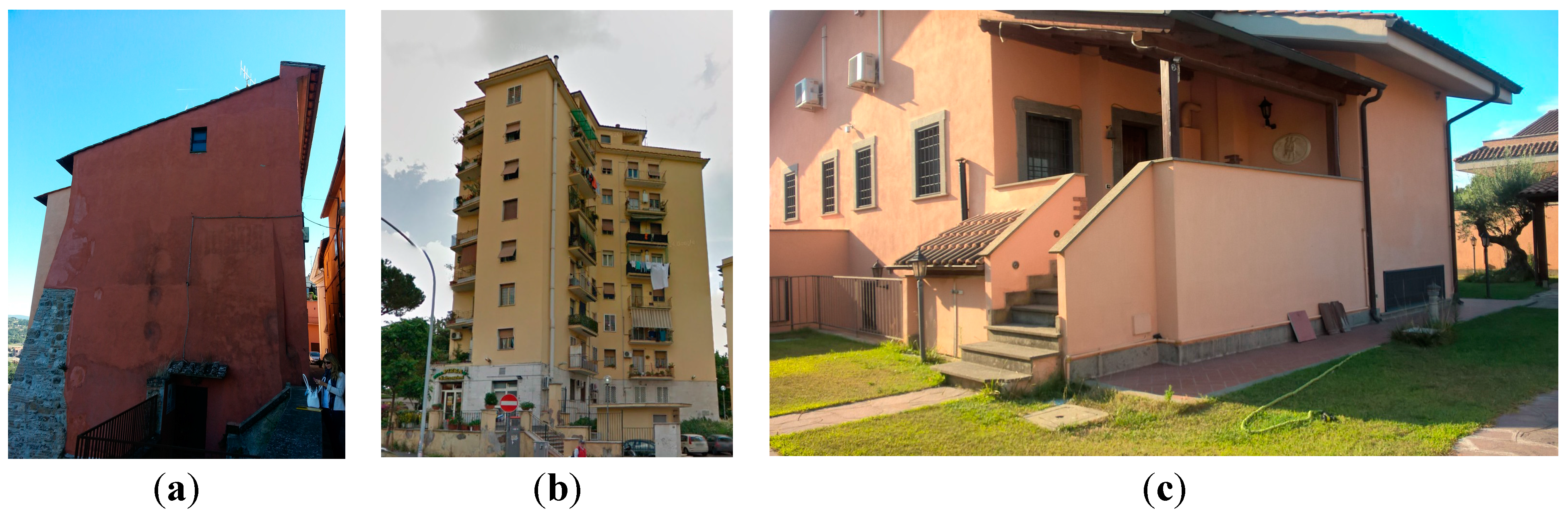
- ▪
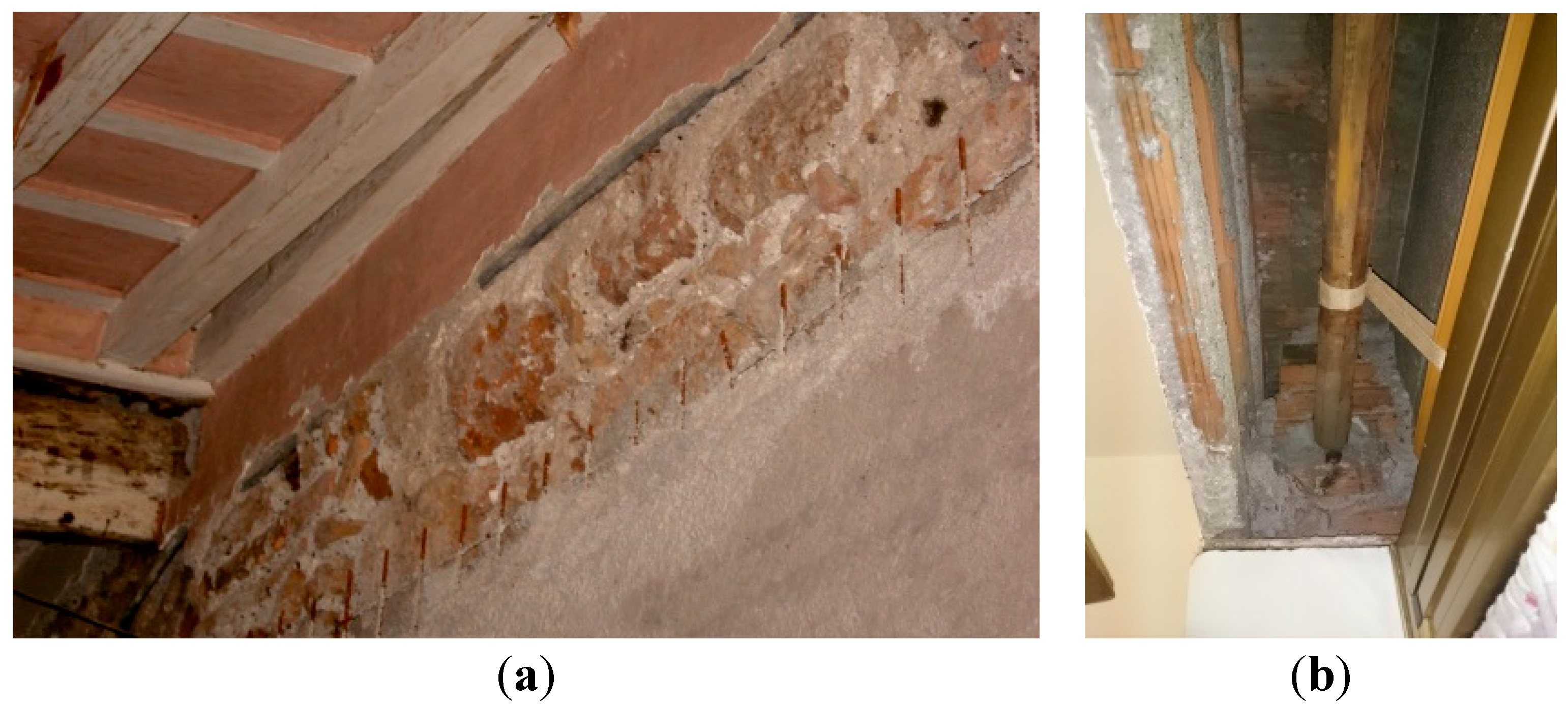
- Case 1—an old building that dates back to the late 1800s, which is characterized by walls made of tuff blocks;
- ▪
- Case 2—an early-1950s structure, characterized by walls made of hollow bricks and concrete;
- ▪
- Case 3—a house built 15 years ago, of which walls are made of hollow bricks.

| Case 1 | Case 2 | Case 3 | |||
|---|---|---|---|---|---|
| Thickness [m] | Thickness [m] | Thickness [m] | |||
| int | - | int | - | int | - |
| Plaster | 0.01 | ||||
| Plaster | 0.02 | Hollow bricks | 0.37 | Plaster | 0.01 |
| Tuff blocks | 0.51 | Concrete | 0.12 | Hollow brick | 0.30 |
| Plaster | 0.02 | Plaster | 0.01 | Plaster | 0.01 |
| ext | - | ext | - | ext | - |
| Total thickness | 0.55 | Total thickness | 0.51 | Total thickness | 0.32 |
| Material Type | Description | Thermal Conductivity [W/mK] |
|---|---|---|
| Plaster | Gypsum plaster | 0.400 |
| 0.570 | ||
| Gypsum and sand | 0.800 | |
| Concrete and sand | 1.000 | |
| Concrete | Natural aggregates concrete | 1.263 |
| 1.613 | ||
| 2.075 | ||
| Expanded clays concrete | 0.325 | |
| 0.702 | ||
| 0.914 | ||
| Autoclave cellular concrete | 0.168 | |
| 0.310 | ||
| Volcanic inert concrete | 0.580 |
| Case 1 | |||||
| Material description | Thermal conductivity [W/mK] | Thermal conductance [W/m2K] | Rs [m2K/W] | Calculated U-value [W/m2K] | |
| int | - | - | - | 0.13 | 1.897 |
| Plaster | Lime and plaster | 0.700 | - | - | |
| Tuff blocks | Tuff | 1.700 | - | - | |
| Plaster | Lime and plaster | 0.700 | - | - | |
| ext | - | - | - | 0.04 | |
| Case 2 | |||||
| Material description | Thermal conductivity [W/mK] | Thermal conductance [W/m2K] | Rs [m2K/W] | Calculated U-value [W/m2K] | |
| int | - | - | - | 0.13 | |
| Plaster | Lime and plaster | 0.700 | - | - | |
| Hollow bricks | Hollow bricks | 0.346 | 0.935 | - | |
| Concrete | Natural aggregates concrete | 1.263 | - | - | 0.734 |
| 1.613 | - | - | 0.745 | ||
| 2.075 | - | - | 0.754 | ||
| Expanded clays concrete | 0.325 | - | - | 0.611 | |
| 0.702 | - | - | 0.695 | ||
| 0.914 | - | - | 0.715 | ||
| Autoclave cellular concrete | 0.168 | - | 0.504 | ||
| 0.310 | - | - | 0.604 | ||
| - | - | ||||
| Volcanic inert concrete | 0.580 | - | - | 0.678 | |
| Plaster | Lime and plaster | 0.700 | - | - | |
| ext | - | - | 0.04 | ||
| Case 3 | |||||
| Material description | Thermal conductivity [W/mK] | Thermal conductance [W/m2K] | Rs [m2K/W] | Calculated U-value [W/m2K] | |
| int | - | - | - | 0.13 | 0.945 |
| Plaster | Lime and plaster | 0.700 | - | - | |
| Hollow brick | Hollow bricks | 0.349 | 1.163 | - | |
| Plaster | Lime and plaster | 0.700 | - | - | |
| ext | - | - | - | 0.04 |
4. Results and Discussion

| Description | Calculated U-Value [W/m2K] | Measured U-Value [W/m2K] | Difference Calculated-Measured [%] | |
|---|---|---|---|---|
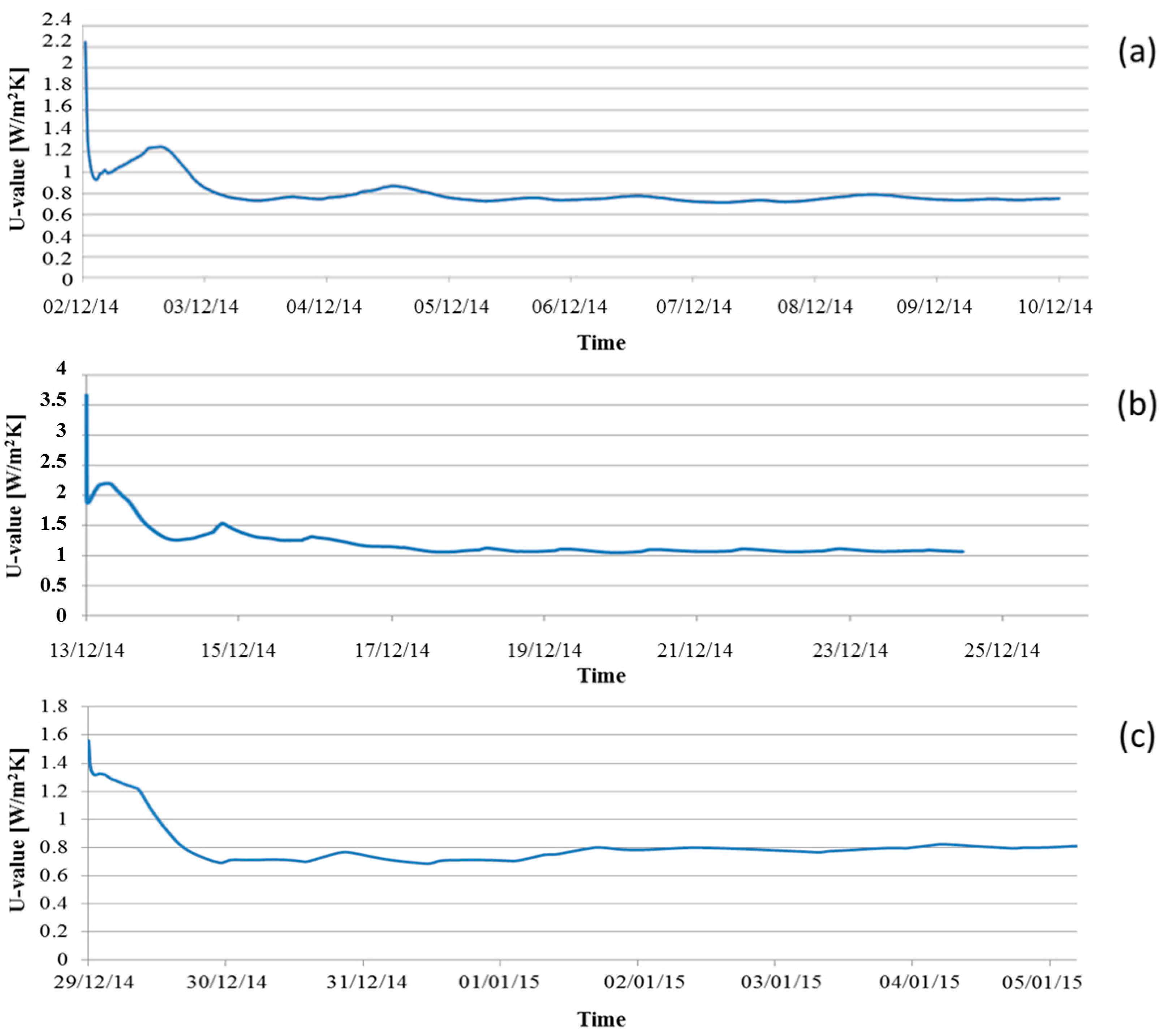
| Case 1 | 1.897 | 0.750 | +153 | |
| Case 2 | Natural aggregates concrete | 0.734 | 1.072 | −32 |
| 0.745 | 1.072 | −31 | ||
| 0.754 | 1.072 | −30 | ||
| Expanded clays concrete | 0.611 | 1.072 | −43 | |
| 0.695 | 1.072 | −35 | ||
| 0.715 | 1.072 | −33 | ||
| Autoclave cellular concrete | 0.504 | 1.072 | −53 | |
| 0.604 | 1.072 | −44 | ||
| Volcanic inert concrete | 0.678 | 1.072 | −37 | |
| Case 3 | 0.945 | 0.810 | +17 |
5. Conclusions
Author Contributions
Conflicts of Interest
References
- Friedman, C.; Becker, N.; Erell, E. Energy retrofit of residential building envelopes in Israel: A cost benefit analysis. Energy 2014, 77, 183–193. [Google Scholar] [CrossRef]
- Evangelisti, L.; Battista, G.; Guattari, C.; Basilicata, C.; de Lieto Vollaro, R. Influence of the thermal inertia in the European simplified procedures for the assessment of buildings’ energy performance. Sustainability 2014, 6, 4514–4524. [Google Scholar] [CrossRef]
- De Lieto Vollaro, R.; Guattari, C.; Evangelisti, L.; Battista, G.; Carnielo, E.; Gori, P. Building energy performance analysis: A case study. Energy Build. 2015, 87, 87–94. [Google Scholar] [CrossRef]
- Gugliermetti, F.; Bisegna, F. Saving energy in residential buildings: The use of fully reversible windows. Energy 2007, 32, 1235–1247. [Google Scholar] [CrossRef]
- De Lieto Vollaro, R.; Calvesi, M.; Battista, G.; Evangelisti, L.; Botta, F. Calculation model for optimization design of the low impact energy systems for the buildings. Energy Procedia 2014, 48, 1459–1467. [Google Scholar] [CrossRef]
- Battista, G.; Evangelisti, L.; Guattari, C.; Basilicata, C.; de Lieto Vollaro, R. Buildings energy efficiency: Interventions analysis under a smart cities approach. Sustainability 2014, 6, 4694–4705. [Google Scholar] [CrossRef]
- Foucquier, A.; Robert, S.; Suard, F.; Stéphan, L.; Jay, A. State of the art in building modelling and energy performances prediction: A review. Renew. Sustain. Energy Rev. 2013, 23, 272–288. [Google Scholar] [CrossRef]
- Baldinelli, G.; Asdrubali, F.; Baldassarri, C.; Bianchi, F.; D’Alessandro, F.; Schiavoni, S.; Basilicata, C. Energy and environmental performance optimization of a wooden window: A holistic approach. Energy Build. 2014, 79, 114–131. [Google Scholar] [CrossRef]
- Pisello, A.L.; Rossi, F.; Cotana, F. Summer and winter effect of innovative cool roof tiles on the dynamic thermal behavior of buildings. Energies 2014, 7, 2343–2361. [Google Scholar] [CrossRef]
- Baldinelli, G.; Bianchi, F. Windows thermal resistance: Infrared thermography aided comparative analysis among finite volumes simulations and experimental methods. Appl. Energy 2014, 136, 250–258. [Google Scholar] [CrossRef]
- UNI 10351:1994—Building materials. Thermal conductivities and vapor permeabilities (in Italian: Materiali da costruzione. Conduttività termica e permeabilità al vapore). Availaible online: www.uni.com (accessed on 30 July 2015).
- UNI 10355—Walls and floors—Values of thermal resistance and calculation methods (In Italian: Murature e solai—Valori della resistenza termica e metodi di calcolo). Availaible online: www.uni.com (accessed on 30 July 2015).
- Baker, P. U-Values and Traditional Buildings. In Situ Measurements and Their Comparison to Calculated Values; Historic Scotland Technical Paper 10; Historic Scotland: Edinburgh, UK, 2011.
- Ghazi Wakili, K.; Binder, B.; Zimmermann, M.; Tanner, Ch. Efficiency verification of a combination of high performance and conventional insulation layers in retrofitting a 130-year old Building. Energy Build. 2014, 82, 237–242. [Google Scholar] [CrossRef]
- Cabeza, L.F.; Castell, A.; Medrano, M.; Martorell, I.; Pérez, G.; Fernández, I. Experimental study on the performance of insulation materials in Mediterranean construction. Energy Build. 2010, 42, 630–636. [Google Scholar] [CrossRef]
- Zarr, R.R. A history of testing heat insulators at the national institute of standards and technology. ASHRAE Trans. 2001, 107, 661–671. [Google Scholar]
- Asdrubali, F.; Baldinelli, G.; Bianchi, F.; Sambuco, S. A comparison between environmental sustainability rating systems LEED and ITACA for residential buildings. Build. Environ. 2015, 86, 98–108. [Google Scholar] [CrossRef]
- International Organization for Standardization (ISO). Thermal Insulation—Building Elements—In-situ Measurement of Thermal Resistance and Thermal Transmittance; ISO 9869-1:2014; ISO: Geneva, Switzerland, 2014. [Google Scholar]
- Desogus, G.; Mura, S.; Ricciu, R. Comparing different approaches to in situ measurement of building components thermal resistance. Energy Build. 2011, 43, 2613–2620. [Google Scholar] [CrossRef]
- Asdrubali, F.; D’Alessandro, F.; Baldinelli, G.; Bianchi, F. Evaluating in situ thermal transmittance of green buildings masonries—A case study. Case Stud. Constr. Mater. 2014, 1, 53–59. [Google Scholar] [CrossRef]
- De Lieto Vollaro, R.; Evangelisti, L.; Carnielo, E.; Battista, G.; Gori, P.; Guattari, C.; Fanchiotti, A. An Integrated Approach for an Historical Buildings Energy Analysis in a Smart Cities Perspective. Energy Procedia 2014, 45, 372–378. [Google Scholar] [CrossRef]
- UNI EN ISO 6946—Building components and building elements—Thermal resistance and thermal transmittance. Availaible online: www.uni.com (accessed on 30 July 2015).
- Gutschker, O. Parameter identification with the software package LORD. Build. Environ. 2008, 43, 163–169. [Google Scholar] [CrossRef]
- Gori, P.; Bisegna, F. Thermophysical parameter estimation of multi-layer walls with stochastic optimization methods. Int. J. Heat Technol. 2010, 28, 109–116. [Google Scholar]
- Heat Flow Meter Model TESTO 435-2. Available online: http://www.testo.it/dettagli_prodotto/0563+4352/testo-435-2-Strumento-multifunzione (accessed on 20 January 2015).
- Clauser, C.; Huenges, E. Rock Physics & Phase Relations: A Handbook of Physical Constants; Ahrens, T.J., Ed.; AGU Reference Shelf Series; American Geophysical Union: Washington, DC, USA, 1995; Volume 3, pp. 105–126. [Google Scholar]
© 2015 by the authors; licensee MDPI, Basel, Switzerland. This article is an open access article distributed under the terms and conditions of the Creative Commons Attribution license (http://creativecommons.org/licenses/by/4.0/).
Share and Cite
Evangelisti, L.; Guattari, C.; Gori, P.; Vollaro, R.D.L. In Situ Thermal Transmittance Measurements for Investigating Differences between Wall Models and Actual Building Performance. Sustainability 2015, 7, 10388-10398. https://doi.org/10.3390/su70810388
Evangelisti L, Guattari C, Gori P, Vollaro RDL. In Situ Thermal Transmittance Measurements for Investigating Differences between Wall Models and Actual Building Performance. Sustainability. 2015; 7(8):10388-10398. https://doi.org/10.3390/su70810388
Chicago/Turabian StyleEvangelisti, Luca, Claudia Guattari, Paola Gori, and Roberto De Lieto Vollaro. 2015. "In Situ Thermal Transmittance Measurements for Investigating Differences between Wall Models and Actual Building Performance" Sustainability 7, no. 8: 10388-10398. https://doi.org/10.3390/su70810388
APA StyleEvangelisti, L., Guattari, C., Gori, P., & Vollaro, R. D. L. (2015). In Situ Thermal Transmittance Measurements for Investigating Differences between Wall Models and Actual Building Performance. Sustainability, 7(8), 10388-10398. https://doi.org/10.3390/su70810388