Article

Optimal Intra-Urban Hierarchy of Activity Centers—A Minimized Household Travel Energy Consumption Approach

Department of Urban Planning, Tsinghua University, Haidian District, Beijing100084, China
*
Author to whom correspondence should be addressed.
Sustainability 2015, 7(9), 11838-11856; https://doi.org/10.3390/su70911838
Submission received: 2 July 2015 / Revised: 13 August 2015 / Accepted: 18 August 2015 / Published: 26 August 2015
(This article belongs to the Special Issue Towards True Smart and Green Cities?)

Abstract

:
An intra-urban hierarchy of activity centers interconnected by non-motorized and public transportation is broadly believed to be the ideal urban spatial structure for sustainable cities. However, the proper hinterland area for centers at each level lacks empirical study. Based on the concentric structure of everyday travel distances, working centers, shopping centers, and neighborhood centers are extracted from corresponding types of POIs in 286 Chinese cities at the prefectural level and above. A U-shaped curve between Household Transportation Energy Consumption (HTEC) per capita and center density at each of the three levels has been found through regression analysis. An optimal intra-urban hierarchy of activity centers is suggested to construct energy-efficient cities.

1. Introduction

One of the most important features of an urban landscape is the clustering of economic activity in many centers of different tiers [1,2]. This has been amply investigated at the regional level, using cities and towns as solid points and seeking their scale distribution within an interurban hierarchy [2,3,4,5,6,7]. Yet, a city should be viewed not only as a physical entity, but also as a pattern of point locations connected by flows of people, information, money, and commodities, as stated in the theory of The Urban Field [8]. Just as there are systems of cities, the cities embedded in these systems are systems themselves [9]. An intra-urban hierarchy of centers with different tiers requires the same attention as has been paid to studies of the interurban hierarchy.
The spatial arrangement of intra-urban centers is closely connected with individual travel behavior. A clear movement hierarchy from an individual’s local stop, district center, and main city center is usually followed during an individual’s everyday commuting from home to city center [10]. It is becoming widely believed that a hierarchy of centers interconnected by non-motorized and public transportation is the ideal urban spatial structure for sustainable cities to reduce dependence on the automobile. In such a hierarchy, a center of a higher level is surrounded by several lower-level centers [11,12,13]. However, the proper quantifiable spatial extent for the centers at each level lacks empirical proof [14], since almost all existing work related to urban spatial structures and Household Transportation Energy Consumption (HTEC) has been limited on the binary choice between monocentricity and polycentricity. Very few studies have investigated whether a U-shape curve exists between HTEC and center density (the number of centers divided by the urbanized area). To achieve our assumption (Section 2), centers of different levels are determined, and HTEC data is gathered with relatively reliable methods (Section 3). Regression analysis between HTEC and center density for each level is conducted to test the existence of the U-shaped curve (Section 4). Finally, some suggestions and discussion are given in Section 5.

2. Literature and Assumptions

2.1. Intra-Urban Hierarchy of Activity Centers and Their Spatial Arrangement

Matters and activities spatially cluster around centers of different tiers in various natural and social phenomena [3]. The same spatial patterns exist at the intra-urban level [2,4,15,16]. Activity centers at different levels cover unique spatial extents and function with different efficient sizes [17,18].
The proper quantifiable spatial extent for centers at each level within the intra-urban hierarchy is crucial for urban planning [19]. Numerous attempts have been carried out to achieve a proper urban spatial structure throughout the twentieth century [3,20,21,22,23,24]. New Urbanism, which emphasized the spatial scale of the basic development unit, has gained growing attention and support since it was proposed in the early nineteen nineties. Transit Oriented Development (TOD) advocates that a neighborhood around a public transport stop should lie within a 2000 feet (600 m) radius, and that a higher-level development unit should be within a one mile extent [25].
Influenced by New Urbanism, more and more research has attempted to restructure spatially-disordered cities by implanting non-motorized and public transportation networks. Cervero [13] advocates that dynamic second-level and third-level centers connected by multilevel transport networks should be constructed step-by-step in a process of urban spatial extension; in this way, an individual’s need to travel to various destinations and distances would be fulfilled. Borrowing from Maslow’s Hierarchy of Needs, Frey [11] demonstrated that both the micro and macro spatial structures of a sustainable city are exemplified by Glasgow. Basically, a center of a higher level is surrounded by several lower-level centers and all are connected by public transportation. Newman and Kenworthy [12] illustrated the intra-urban hierarchy of four levels in the Sydney metropolitan area. There, the local center is the lowest level, covering an extent of 3 km2 and serving 8000–19,000 people. The town center, the higher level, covers about 30 km2 and serves 70,000–175,000 people. The transit city center usually features a spatial extent of 20–30 km in radius. Finally, the Central Business District (CBD) is the highest level. Dai [26] summarized related studies on intra-urban hierarchy and put forward a serious of suggestions about the scale of each level in the intra-urban hierarchy for Chinese cities. However, the author himself admitted that his suggestions were based on strictly ideal assumptions that lacked of empirical study or proof. This is the common defect of all similar works.

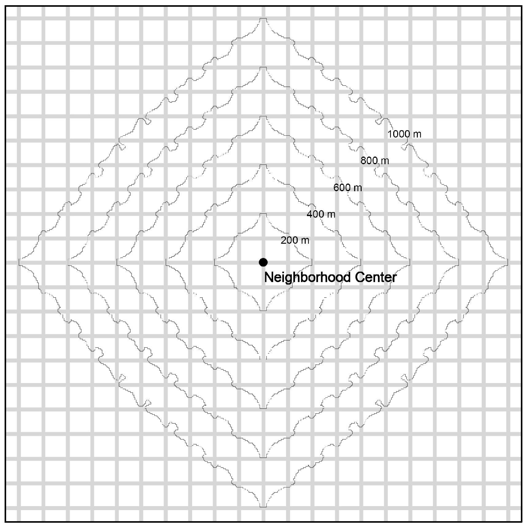
2.2. Concentric Structure of Everyday Trip Space

The intra-urban hierarchy of activity centers is closely connected with individual travel behavior [14]. Individual travel destinations (mainly shopping trips) are usually spatially-distributed in a concentric structure [27,28,29,30,31], because preferences of travel time and mode are dissimilar for different types of activities, which can be explained by the travel time ratio (TTR) index [32,33]. The rationale behind the TTR concept is that the location where an individual will participate in an out-of-home activity is related, among other things, to the travel time investment needed to reach the activity location, as well as the duration of the activity to be conducted at that destination. Susilo and Dijst [34] used the Dutch National Travel Survey to measure the TTR index for various activities. The results show that each activity has a unique TTR index; for example, the TTR for work is about 0.12 (one hour of travel for work in accordance with an eight-hour workday). For daily product shopping, the TTR is roughly 0.4 (a 12-minute shopping trip in accordance with 30 min of shopping), and it is approximately 0.23 for travel to a café/restaurant (20 min of travel in accordance with a 90-minute outing at the café/restaurant).
The concentric structure of everyday trip spaces is mostly investigated in terms of shopping trips. Berry and Parr [35] improved the traditional Central Place Theory by bringing in consumer behavior to explain the hierarchical structure of commercial activities. Wu et al. [36] conducted a questionnaire survey in Tianjin, discovering an obvious hierarchical structure of shopping trips, in which average shopping trips for food and vegetables is 0.4 km, for daily necessities is 1 km, for shirts and socks is 2 km, for household appliances is 5 km, and for suits and overcoats is 7.4 km. Feng et al. [37] detected a similar concentric pattern for Beijing’s residents; i.e., average shopping trips for food and vegetables is 1.07 km, for daily necessities is 1.43 km, for clothes is 4.04 km, and for household appliances is 5.2 km.
Trips for work are usually longer than for daily shopping, which can be explained by the TTR concept, since work duration greatly exceeds that of ordinary shopping activities. The constant Travel-Time Budgets (TTBs) Hypothesis is of great help in understanding individual commuting behavior. A TTB simply means that people allocate a fixed portion of the 24 h they have in a day as the maximum amount of time out of that day that they would be willing on average to spend on travel [38]. After being first introduced by Tanner in 1961 [39], the TTB has been reported almost as a universal constant across time and space at 1–1.3 hours per person per day, e.g., 70.7 min [40], 70–90 min [41], 68 min [42], 78 min [43], and 60–80 min [44]. Generally, automobile and public transportation are the chief modes for commuting. Dieleman et al. [45] determined that 48% of people commute by car, and by comparison make only 30% of shopping trips by car, in the Netherlands. Zhou and Yang [46] analyzed the commuting behavior of residents in Guangzhou, China, and found that the bus is the primary mode for commuting, with 31.5% of people using it with an average commuting distance by bus of 5.5 km. The automobile was next, with 24% with the average trip length of 4.9 km, and the bicycle was last, with 20% using it and the average trip bicycle trip length was 3.0 km.
Trips for leisure and social activities are usually longer and more automobile-dependent. According to Frandberg and Vilhelmson [47], the average trip length for visits in Sweden is 24.1 km, and for leisure is 20.4 km; both of these are longer than shopping trips (9.0 km) and work trips (16.8 km). Burger et al. [48] discovered that 47% of social activities and 38% of leisure activities take place out of the municipality in which one lives in Randstad, Holland. As a comparison, only 22% of shopping activities were outside of the municipality in which an individual in Randstad lives.

2.3. Interrelations between Travel Mode Choice and Trip Distance

With varying operational speed, accessibility, cost, and comfort levels, each transport mode is suited for a unique optimal trip distance. Van Wee et al. [39] visualized the relationship between trip distance and transport mode with a theoretical model, taking the speed, cost, and comfort level of different transport modes into consideration. Miao and Zhao [49] illustrated this issue similarly. Scheiner [50] reported findings from longitudinal analyses of the German national travel survey KONTIV for the period 1976–2002, and suggested that once the availability of the car is held constant, the rationale behind people’s choice of travel mode for a certain trip distance remained relatively stable. It is shown that the proportion of walking is extremely high for trips shorten than 1 km, and the proportion of automobile travel increases gradually for trips longer than 1 km. The advantageous trip distance for a bicycle is 1–3 km, and for public transport it is 5–7 km. Liu et al. [51] built a programming model of inhabitant trip distance distribution under the constraints of various utilities; they targeted information entropy maximization and validated the model using inhabitant trip survey data from Suzhou. The result shows similar advantageous trip distance for different types of transport mode with Scheiner’s study [50]. Santos et al. [52] summarized the factors that impacted the choice of transport mode, including social-economic and urban form factors, and tested them with a sample of 112 medium-sized European cities using a discrete choice modeling approach.
Detailed discussion of the advantageous trip distance of each specific transport mode is carried out by a large body of literature. Millward et al. [53] analyzed the frequency and length of walking episodes, categorized by origin, purpose, and destination, and also investigated the distance-decay function for major destinations for walking behaviors in Halifax, Canada. It was found that most walks are shorter than 600 m, and very few exceed 1200 m. Heinen et al. [54] summarized existing literature on commuting by bicycle, pointing out that for distances between 0.5 and 3.5 km, the bicycle is most often used [55,56], and noting that the “acceptable” maximum travel distance differs between genders: 11.6 km for men and 6.6 km for women [57]. Roth et al. [14] utilize the large-scale, real-time “Oyster” card database of individual person movements in the London subway to reveal the structure and organization of the city. It is shown that intra-urban movement is strongly heterogeneous in terms of volume, but not in terms of distance travelled; an interval of 5–10 km was found to be the peak interval for subway trips. Wang et al. [58] explored the mobility patterns of passengers in a public transport network based on Shijiazhuang bus passenger survey data. The results show similar peaked distribution of travel distance, which can be fitted by a negative binomial distribution, and the peak point for a bus trip is approximately 4–5 km. Ben-Akiva and Morikawa [59] estimated models of choice among alternative travel modes using revealed preference data and stated preference data. The main conclusion is that there is no evident preference for rail travel over bus when quantifiable service characteristics such as travel time and cost are equal, but a bias does arise when rail travel offers a higher-quality service.

2.4. Monocentricity vs. Polycentricity: Debate about Urban Spatial Structure’s Impact on HTEC

Large cities and urban regions are now typically described as polycentric (multi-centered), having evolved from monocentric (single-centered) entities in the presence of enhanced transport and communication technologies, rising affluence, and the decentralization of activities [1,45,60]. An extensive literature has developed over the last quarter century documenting relationships between travel behavior and patterns of urbanization [61,62,63]. However, empirical findings have been quite inconsistent about whether a monocentric or polycentric urban spatial structure tends to help reduce HTEC, as summarized by Buliung and Kanaroglou [64] in a comprehensive literature review on this issue.
Generally, the urban spatial structure impacts HTEC in two ways: one is the mode choice and the other is the travel distance and duration. Findings with respect to travel mode and polycentricity have been relatively consistent, implying that the polycentric urban form tends to be associated with higher levels of auto dependence and solo driving. This can be partially explained by (a) insufficient residence–workplace public transit connectivity in polycentric cities and (b) discretionary activities for residents being located in peripheral and/or suburban locations [45,65,66,67,68,69,70,71]. On the other hand, findings have been relatively inconsistent about polycentricity’s impact on trip length and duration. Supporters of polycentricity use the co-location hypothesis to describe the potential commuting implications of firm and household decentralization. Under co-location, efficient travel is thought to emerge as firms and households follow one another during the course of employment decentralization [70,72,73,74,75,76]. Supporters of monocentricity argue that even when the number of jobs and housing units in an area are equal, there is no guarantee that the people who work in an area are the same ones who live there, since a large number of empirical evidence shows that the emergence of the polycentric urban form has not led to system-wide travel efficiencies for work and other purposes [45,65,66,67,69,70,71]. Maat et al. [77] indicate that a commute time of 15 to 20 min is acceptable to many people, so they do very little to further reduce their commutes. Moreover, according to the utility theory, distance is not the only constraint on travel behavior; the benefit of shopping at a higher-quality store, for example, may outweigh distance considerations, and one might travel longer to buy better or cheaper products at a place that offers a diversity of products rather than to patronize a more limited option located nearby.

2.5. Theoretical Assumptions

This review of the ideal conception of the intra-urban hierarchy of activity centers interconnected by non-motorized and public transportation shows that there is a need for empirical studies on quantifiable spatial extents for centers at each level based on the concentric structure of everyday trip space and the advantageous trip distance of each transport mode. As mentioned above, polycentricity is believed to be associated with higher levels of auto dependence, yet at the same time the average commuting distance may be shorter, based on the co-location hypothesis in polycentric cities. As an overlying result of both transport mode and travel distance, HTEC may feature a quadratic relationship with the average hinterland area of a center. If a center covers a vast hinterland (resembling the monocentric situation), residents at the distant periphery have to make longer commuting trips, leading to increased HTEC. On the other hand, if a center covers a small hinterland (resembling the polycentric situation), residents tend to rely on the more flexible automobile mode as a result of insufficient residence–workplace public transit connectivity. For centers at each level within the intra-urban hierarchy, there may always exist a U-shaped curve between HTEC and the center density (the reciprocal of the average hinterland area of a center), implying that centers at each level have an optimal hinterland range.
The concentric structure of everyday trip spaces underlies the classification of center levels within the intra-urban hierarchy. Trips conducted for daily products, kindergarten, primary school and to a community center are usually within a 10-minute walk (half a mile, 800 m); i.e., this represents the first concentric layer (Neighborhood Center), resembling the concept of the Neighborhood Unit presented by Perry [23]. The main activities in the second concentric layer (Shopping Center) are non-daily shopping, service, and going out for dinner, most of which takes place within the desirable distance of 10–20 minute bicycling. In the third concentric layer (Working Center), companies and places of leisure activities such as friends’ home, theaters, and museums are the major destinations of individuals, and public transport (by bus or subway within the desirable time budget of 30 min) is the ideal mode for the third concentric layer. A U-shaped curve is assumed to exist at each of the three levels.

3. Methods and Data

Theoretical assumption testing is conducted in the following three steps.

3.1. Extraction of Intra-Urban Centers at Each Level

Density thresholding based on employment is the mainstream effective method for quantitative definitions of intra-urban centers [14]. Thurstain-Goodwin and Unwin [78] illustrated how to extract intra-urban centers of UK towns using kernel density estimation to transform the data from point or area “objects” into continuous surfaces of spatial densities. Following this method, we attempt to extract working, shopping and neighborhood centers of 286 Chinese cities at the prefectural level and above, based on different types of points of interest (POI) obtained from Open Street Map [79]. The POIs have been supplemented and checked based on the Baidu Map [80] and reclassified into 31 sub-groups included in seven groups (Table 1).
Table 1. Description of groups and sub-groups for all the POIs for the 286 Chinese cities at the prefectural level and above.
GroupSub-GroupNote
ShoppingDaily shoppingIncluding grocery store and small supermarket
Vegetable market
Mall and supermarketIncluding shopping mall and big supermarket
Pharmacy
Non-daily shoppingAll the other shopping facilities except the above four groups
DiningRestaurantIncluding Chinese restaurant and foreign restaurant
Beverage shopIncluding café and teahouse
Fast food
Cake and bread
EducationKindergarten
Primary school
Middle school
University
HealthHospital
Clinic
LeisureSports
Park
MuseumIncluding all kinds of museums and galleries
Theater and cinema
KTV
Bar
ServicePost office
Telecom shopSuch as China Mobile and China Unicom
Bank
Dry cleaners
Barber shop
Hotel
JobCommercial building
Company
Factory
Government facilities
Density analysis with point-based activities for center extraction refers implicitly to the CBD research developed during the second half of the twentieth century, and a set of activities and indicators has been listed to be considered for an analysis on CBD based on western cities [81,82,83]. Yet spatial distributions of POIs in Chinese cities are different from those in Western cities due to the unique socialist market economy and planning regulations in China: (1) following the regulations of the Standard for Residential Planning published by the Chinese Ministry of Housing and Urban-Rural Development, amenities of basic services and commodities, such as grocery shops, clinics, kindergartens, primary schools, and community centers are usually within good accessibility (within 800 m) for most residents; (2) huge divergence in trip distance between daily shopping and non-daily shopping has been revealed by several studies on the hierarchical structure of shopping activity in Chinese cities [28,36,37]. Trip distance for daily product and food is 1–2 km on average, while for clothing, appliance, and other non-daily products the distance is mostly over 4 km, close to the trip distance for meals and service [27,30]; and (3) with the fast expansion of urbanized areas in these two decades, commuting trip distance is generally longer than non-daily shopping trip distance, indicating that a working center covers larger hinterland than a shopping center in Chinese cities.
Based on the analyses above and the assumptions that the main activities take place in centers at each level, we extract neighborhood centers with the POIs of daily retail, community center, kindergarten, primary school, and clinic (Right in Figure 1). Shopping centers are obtained with the POIs of non-daily retail, restaurant, and service (Middle in Figure 1). Finally, working centers are attained with all the POIs because all the facilities generate jobs (Left in Figure 1).
Figure 1. Exemplification of Beijing for center extractions. (Left) Raster of working facilities in Beijing. (Middle) Raster of shopping facilities in Beijing. (Right) Raster of neighborhood facilities in Beijing.
Sustainability 07 11838 g001
Shopping centers are exemplified here to show the specific process with the following four steps.
(1)
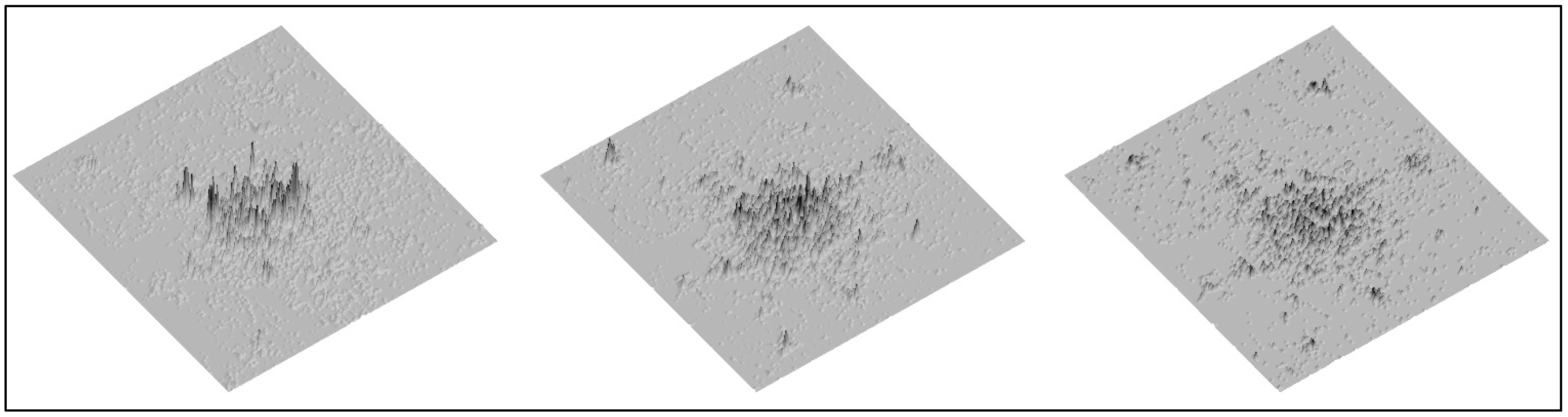
Kernel Density analysis with the search radius of 500 meters is utilized, sourcing from POIs of non-daily retail, restaurant, service, and middle school in ArcMap 10.1. A raster with a 20-meter resolution covering the region of Mainland China is generated. About the bandwidth of kernel density analysis, some similar studies usually use k-order nearest-neighbor analysis to delimitate the bandwidth for each city [84,85]; however, the number of sample cities in our study is much larger, and it will be very difficult to carry out the k-order nearest-neighbor analysis for the 286 sample cities once at a time. We think 500-meter bandwidth is a good choice from a practical point of view: first, the upper limit for walking is usually 800 meters of path distance [50,53], approximately 500 meters of Euclidean distance in a grid city. Second, according to the Standard for Residential Planning published by the Ministry of housing, service radius of basic amenities at neighborhood level, such as bus stops, kindergartens, community centers, and grocery shops is also 800 meters of path distance. Third, the outcome of the bandwidth for Italian cities is 400 m (Trieste) and 389 meters (Udine) through k-order nearest-neighbor analysis (k = 50) [85], considering that blocks in Chinese cities are usually larger than in European cities, 500 meters is quite proper for kernel density analysis in Chinese cities.
(2)
Urbanized areas for each city are identified based on the global urban extent map of MODIS 500 [86] and a Google map with historic versions in Google Earth 6.0.
(3)
A shopping center raster for each city is extracted with the urbanized areas, and reclassified into ten classes based on cell value with the Natural Breaks Method (Natural Breaks classes are based on natural groupings inherent in the data, class breaks are identified that best group similar values and that maximize the differences between classes, from ArcGIS 10.1 [87].
(4)
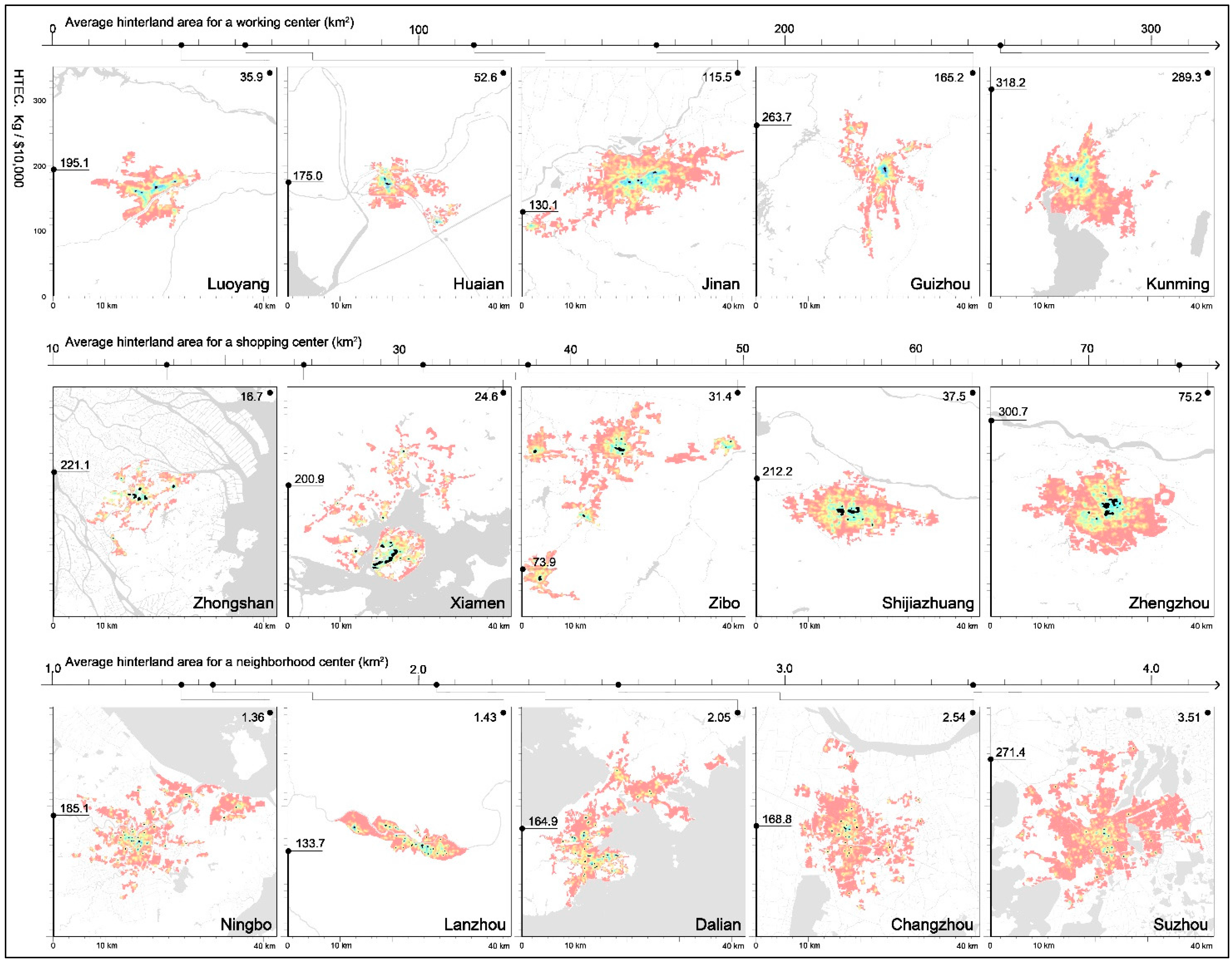
Cells in the top three classes are identified as shopping centers, after comparison with the actual location of shopping centers based on the master plans of Beijing, Shijiazhuang, Jinan, Zhengzhou, Taiyuan, and so on (Figure 2).
Similarly, working centers and neighborhood centers are obtained (Figure 2). Cells in the top one class of the working center density raster are identified as working centers, while cells in the top five classes of neighborhood centers of the neighborhood center raster are recognized as neighborhood centers, after comparison with actual positions of neighborhoods based on the master plans of cities mentioned above.
Figure 2. Extraction results of working centers (upper), shopping centers (middle) and neighborhood centers (lower). Black stands for centers, red stands for cells with lower value, and blue stands for cells with higher value.
Sustainability 07 11838 g002

3.2. Estimations of HTEC and Obtainment of Controlled Variables

HTEC are estimated with the “Top-down Method” provided by the 2006 IPCC guidelines for national greenhouse gas inventories [88] as showed below.
C = Q1 × L1 × λ1 × EF1/P+ Q2 × L2 × λ2 × EF1/P + E1 × EF6 × Q3/Q'3 × P
C is HTEC per capita. Q1/Q2/Q3 is the amount of urban buses/taxis/private vehicles. Q'3 is the amount of private vehicles in the province where the city lies in. L1/L2 is the annual mileage of buses/taxis. λ12 is the 100 km fuel factor of buses/taxis. EF1/EF1 is the carbon emission factor of diesel oil/gasoline. E1 is the household gasoline consumption of the province where the city lies in.
Formula parameters are obtained from a variety of sources. They include: (1) urban buses/taxis/private vehicles counts and urban population from the China City Statistical Yearbook [89]; (2) carbon emission factor of diesel oil and gasoline from the 2006 IPCC guidelines for national greenhouse gas inventories [88]; (3) household gasoline consumption at the provincial level from the China Energy Statistical Yearbook [90]; and (4) annual bus mileage is obtained from the Beijing Public Transport Group website while bus speed is set at 16 km/h and fuel factor is 32 L/100 km according to Zhang’s research [91]. Taxis are assumed to utilize gasoline as no record exists in any statistical yearbook for percentage of natural gas operated taxis. Annual taxi mileage is set at 12,000 km, and fuel factor is set at 10 L/100 km according to Zhao’s research [92].
GDP per capita, population density, and urbanized area have been proven to feature significant impacts on HTEC per capita by a large body of literature [93,94,95,96,97,98,99] (Statistical description of these variables can be seen in Table 2). For our sample of 286 Chinese cities at the prefectural level and above: (1) the value of GDP per capita is from the China City Statistical Yearbook [89]; (2) the value of the urbanized area is obtained based on the global urban extent map of MODIS 500 [86] and Google maps with historic versions in Google Earth 6.0, as mentioned above; and (3) the population density of the urbanized area is recalculated for urban form metrics based on the population density map with a 100-meter resolution provided by the Worldpop database [100]. This database was chosen because the population density values in the statistical yearbooks do not accurately reflect reality. The statistical yearbook calculation method, which divides the urban population by the area of the entire administrative district, results in a much smaller value of population density than what exists in reality, because the urbanized areas where most citizens settle are usually much smaller than the entire administrative district.
Table 2. Statistical description of center densities, HTEC and controlled variables.
VariablesNMinimumMaximumAverageStandard Deviation
Working center density (numbers/km2)2860.0011.0150.0330.065
Shopping center density (numbers/km2)2860.0031.0150.0440.066
Neighborhood center density (numbers/km2)2860.058.440.76080.83354
HTEC (kg/person)2869.6251071.632139.059104.606
GDP per capita (1,000 Dollars/person)2860.92023.4126.1423.823
Urbanized area (km2)2860.9851465.684109.797181.142
Population density (People/km2)286355.54110,996.6134809.2472216.433

3.3. Regression Analyses between Center Density and HTEC

Great divergences of the urbanized area in our 286 study cities necessitated a regression analysis conducted by grouping based on urbanized area. According to the Notice on Adjusting Classification Standard of City Size published by the Chinese State Council [101], Chinese cities are reclassified into five classes based on urban permanent resident population: small cities with a population under 500,000, medium cities with 500,000 to 1,000,000 people, large cities with 1,000,000 to 5,000,000 people, extra-large cities with a population over 5,000,000 and megacities with over 10,000,000 people. Two adjustments are made based on the above classification: (1) the extra-large cities and megacities are merged into one class, since samples of each are too small to conduct a regression analysis; and (2) large cities are divided into two classes: one with a population of 1,000,000 to 2,000,000 and the other with a population of 2,000,000 to 5,000,000, because the latter class is proven to present the best comprehensive efficiency in China [102,103].
The relationship between the working center density and the natural logarithm (LN, used to eliminate the heteroscedasticity) of HTEC per capita is demonstrated here to exhibit the regression analysis, taking GDP per capita, population density and the urbanized area as controlled variables. A significant quadratic relationship (a U-shaped curve, as shown in Figure 3) between working center density and HTEC per capita is found only in the case of cities with a population of 2,000,000 to 5,000,000 (Table 3). Cities with working center density of 0.0149 (the average hinterland area of a working center is about 67 km2) have the lowest HTEC per capita.
Figure 3. Illustration of the U-shaped curve between HTEC per capita and center densities at all three levels.
Sustainability 07 11838 g003
Table 3. Regression results between HTEC and center densities at each of the three levels for centers. LN HTEC per capita is the dependent variable, coef in the table is short for non-standardized coefficient.
Center LevelAdjusted R2SIGNQuadratic Term OF Center DensityCenter DensityPopulation DensityUrbanized AreaGDP Per CapitaConstant
Working center0.5430.0000334coef2924.12–88.36360.000040.00110.06134.211
sig0.031920.037360.264070.20450.01710
t2.25811–2.185761.139701.29882.53439.482
Shopping center0.5000.0001733coef656.678–40.69590.000040.00130.05954.312
sig0.053180.035680.314840.12960.02010
t2.02203–2.211211.024171.56312.468610.42
Neighborhood center0.3890.0020933coef1.85298–2.415650.000030.00160.03404.312
sig0.073690.096220.472240.07350.22590
t1.86080–1.723600.729061.86171.239110.42
Similarly, the existence of the U-shaped curve is confirmed between HTEC per capita and shopping center density in the class of a 2,000,000 to 5,000,000 population (Table 3). Cities with shopping center density of 0.0313 (the average hinterland area of a shopping center is about 32 km2) have the lowest HTEC per capita. Neighborhood center density is also demonstrated to have a significant quadratic relationship with HTEC per capita in the class of a population of 2,000,000 to 5,000,000, HTEC is the lowest for cities with neighborhood center density of 0.652 (the average hinterland area of a neighborhood center is about 1.53 km2).
It is worth mentioning that only for cities with 2,000,000 to 5,000,000 people, three types of center densities show significant quadratic relationships with HTEC. The entire intra-urban hierarchy is difficult to identify in smaller cities, while the urban spatial structure tends to be disordered and the meso-level spatial unit is generally ignored in megacities [26].

4. Results and Discussion

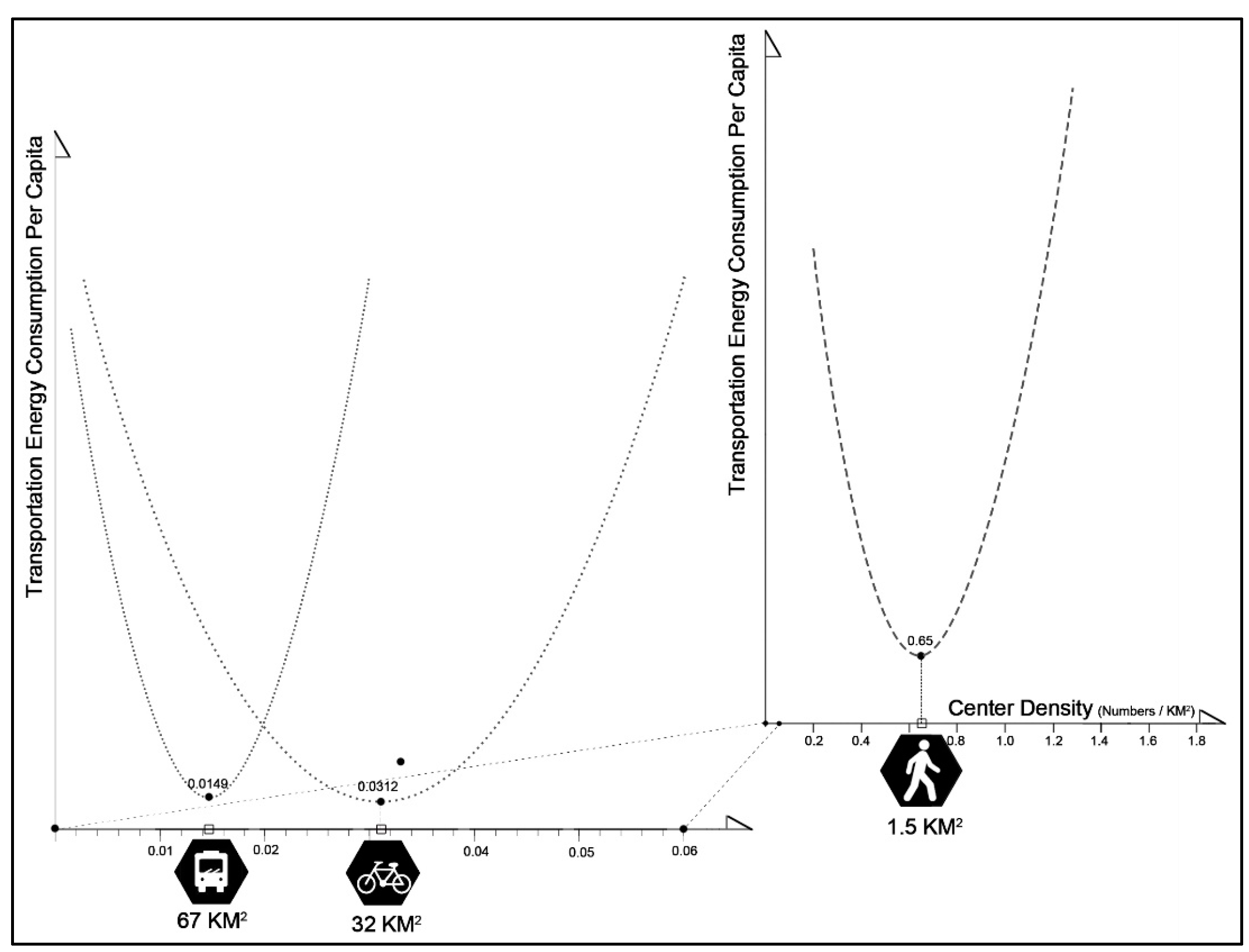
4.1. Neighborhood Center and HTEC

It has been proven by the previously-discussed regression analysis that a neighborhood center covering an average of 1.53 km2 favors reducing HTEC. Hinterlands for centers of small scale within city borders tend to be quadrangular rather than hexagonal, as typically described in the Central Place Theory, since the isochrones starting from any point in grid cities are mostly quadrangular at 45-degree angles to the grid [104] (Figure 4). We can see that the distance from the centroid (a neighborhood center) to a vertex is about 880 meters for a square of 1.53 km2 (Figure 3), meaning that any point within the square is less than 880 meters away from the neighborhood center. This hinterland range resembles the Neighborhood Unit of a half-mile radius presented by Perry [23]. High accessibility of daily products and services within 800 meters (a 10-minute walk) has been proven to significantly lower the HTEC per capita by encouraging non-commuting trips on foot [93,94,96]. A desirable distance of less than 800 meters for walking determines that some residents in a neighborhood unit larger than 1.53 km2 have to drive to obtain daily products; on the other hand, incomplete facilities in centers smaller than 1.53 km2 would also force residents to drive to centers at a higher level to find the products they need.
Figure 4. Isochrones starting from a neighborhood center in grid cities, speed for non-road area is set as half of that for road (the orthogonal grey lines), and the distance between road axes is set as 100 meters.
Sustainability 07 11838 g004

4.2. Shopping Center and HTEC

From the regression analysis discussed above, we find that 32 km2 is the optimal hinterland area of a shopping center for the purpose of the lowest HTEC. It can be concluded that the shape of the optimal shopping center’s hinterland is a square, resembling the optimal neighborhood unit described above, but about five times larger, since the distance from the centroid to a vertex for the optimal shopping center’s hinterland (4 km2) is about 5 times that of the optimal neighborhood center’s hinterland (0.88 km2). In such a hinterland, any point is within 4 km of any other point, starting from the centroid (the shopping center); this is close to the upper limit of the desirable trip distance using the bicycle mode [55,56]. A shopping center with a larger hinterland will mean that some residents in the periphery have to drive or take the bus to the shopping center, which is more energy-consuming than if they could travel by bicycle. Additionally, sometimes the products and services available at a shopping center with a smaller hinterland are undesirable, causing residents to make trips to centers at higher levels that are farther away.

4.3. Working Center and HTEC

For working centers, the ideal hinterland area is 67 km2, exactly two times of that for shopping centers. According to Berry and Parr [35], the ratio (k) of the hinterland area between one level and the lower level may be two, four or nine in quadrangular central place systems. Based on the situation of k = 2, the hinterland for a working center would be a square of 8.2 km per side parallel to the road grid, the vertex of which is located within a shopping center (Figure 5). Residents in such a working center’s hinterland would travel at most 5.7 km to the working center, which is still in the desirable distance range of buses, since none of the 35 Chinese cities with 2,000,000 to 5,000,000 people in our sample featured a subway system in 2010 (the base year of the regression). This conclusion suggests that, for cities featuring faster public transport systems, e.g., subway or suburban railway, the optimal hinterland of a working center way be larger, which calls for further investigation with samples all around the globe, because the number of cities featuring subway or suburban railways in any one country is too small to conduct a proper regression analysis.
Figure 5. Illustration of the optimal intra-urban hierarchy of activity centers tested in this article.
Sustainability 07 11838 g005

5. Conclusions

Numerous attempts have been carried out since Howard’s Garden City Theory in 1898 to achieve a proper urban spatial structure. An ideal intra-urban hierarchy of activity centers interconnected by non-motorized and public transport for sustainable cities has been proposed, conceived and advocated many times, yet the proper quantifiable spatial extents for centers at each level in terms of controlling HTEC still lack empirical proof. Based on the concentric structure of everyday trip space, working centers, shopping centers, and neighborhood centers are extracted from corresponding types of POIs in 286 Chinese cities at the prefectural level and above. The U-shaped curve between HTEC per capita and center densities in each of the three levels has been found through regression analysis. For the purpose of achieving the lowest HTEC per capita, the optimal hinterland area is 67 km2 for a working center with the bus as the preferred transport mode, 32 km2 for a shopping center with the bicycle as the preferred transport mode, and 1.53 km2 for a neighborhood center with walking as the preferred transport mode (Figure 5). Thus, an optimal intra-urban hierarchy of activity centers emerges, yet probable centers at higher levels in larger cities calls for further investigation from a global perspective.

Acknowledgments

This work was supported by the following research projects: Form and Design of Energy-efficient Neighborhood in Megacities in Southern Region of North China funded by Independent Research Program of Tsinghua University (No. 20111081052); Low Carbon Urban Design–From Options Assessment to Policy Implementation funded by the Low Carbon Energy University Alliance (No. 2011LC002).

Author Contributions

Jie Zhang put up with the original idea, made explanations about the regression results and checked the manuscript. Yang Xie complemented the theoretical assumptions, finished the literature reviews, and carried out the data collection and regression analysis.

Conflicts of Interest

The authors declare no conflict of interest.

References

  1. Anas, A.; Arnott, R.; Small, K.A. Urban spatial structure. J. Econ. Lit. 1998, 36, 1426–1464. [Google Scholar]
  2. Batty, M. The size, scale, and shape of cities. Science 2008, 319, 769–771. [Google Scholar] [CrossRef] [PubMed]
  3. Christaller, W. Central Places in Southern Germany; Prentice-Hall: London, UK, 1933. [Google Scholar]
  4. Batty, M.; Longley, P.A. Fractal Cities: A Geometry of Form and Function; Academic Press: Waltham, MS, USA, 1994. [Google Scholar]
  5. Beckmann, M.J. City hierarchies and the distribution of city size. Econ. Dev. Cult. Change 1958, 6, 243–248. [Google Scholar] [CrossRef]
  6. Carroll, G.R. National city-size distributions what do we know after 67 years of research? Prog. Hum. Geogr. 1982, 6, 1–43. [Google Scholar]
  7. Bettencourt, L.M.A. The origins of scaling in cities. Science 2013, 340, 1438–1441. [Google Scholar] [CrossRef] [PubMed]
  8. Friedmann, J.; Miller, J. The urban field. J. Am. Plan. Assoc. 1965, 31, 312–320. [Google Scholar] [CrossRef]
  9. Berry, B.J. Cities as systems within systems of cities. Pap. Reg. Sci. 1964, 13, 147–163. [Google Scholar] [CrossRef]
  10. Thompson, C.W. Urban open space in the 21st century. Landsc. Urban Plan. 2002, 60, 59–72. [Google Scholar] [CrossRef]
  11. Frey, H. Designing the City: Towards a More Sustainable Urban Form; Spon: London, UK, 1999. [Google Scholar]
  12. Newman, P.; Kenworthy, J. Urban design to reduce automobile dependence. Opolis 2006, 2, 35–52. [Google Scholar]
  13. Cervero, R. The Transit Metropolis: A Global Inquiry; Island press: Washington, DC, USA, 1998. [Google Scholar]
  14. Roth, C.; Kang, S.M.; Batty, M.; Barthélemy, M. Structure of urban movements: Polycentric activity and entangled hierarchical flows. PLoS ONE 2011. [Google Scholar] [CrossRef] [PubMed]
  15. Batty, M. Cities and Complexity: Understanding Cities with Cellular Automata, Agent-Based Models, and Fractals; The MIT press: Cambridge, MS, USA, 2007. [Google Scholar]
  16. Zhou, G.Z. City and Region: A typical open giant complex system. City Plan. Rev. 2002, 2, 7–8. (In Chinese) [Google Scholar]
  17. Richardson, H.W. Optimality in city size, systems of cities and urban policy: A sceptic’s view. Urban Stud. 1972, 9, 29–48. [Google Scholar] [CrossRef]
  18. Capello, R.; Camagni, R. Beyond optimal city size: An evaluation of alternative urban growth patterns. Urban Stud. 2000, 37, 1479–1496. [Google Scholar] [CrossRef]
  19. Mulligan, G.F.; Partridge, M.D.; Carruthers, J.I. Central place theory and its reemergence in regional science. Ann. Reg. Sci. 2012, 48, 405–431. [Google Scholar] [CrossRef]
  20. Doxiades, K.A. Ekistics: An Introduction to the Science of Human Settlements; Hutchinson: London, UK, 1968. [Google Scholar]
  21. Howard, E. To-morrow: A Peaceful Path to Real Reform; Routledge: London, UK, 1898. [Google Scholar]
  22. Krier, L.A.C.M. Rational Architecture: The Reconstruction of the European City; Archives d’architecture moderne: Brussels, Belgium, 1978. [Google Scholar]
  23. Perry, C.A. The neighborhood unit. In Regional Survey of New York and Its Environs; Committee on the Regional Plan of New York and Its Environs: New York, NY, USA, 1929; pp. 34–35. [Google Scholar]
  24. Hall, P.; Ward, C. Sociable Cities: The Legacy of Ebenezer Howard; Wiley: Chichester, UK, 1998. [Google Scholar]
  25. Calthorpe, P. The Next American Metropolis: Ecology, Community, and the American Dream; Princeton Architectural Press: New York, NY, USA, 1993. [Google Scholar]
  26. Dai, D.S. Study on the Hierarchial System of Urban Space and the Pattern of Development Based on Green Transportation. Ph.D. Thesis, Southeast University, Nanjing, China, June 2011. [Google Scholar]
  27. Chai, Y.W.; Shang, Y.R. The study on the temporal-spatial characteristics of the consumer activities of Shenzhen residents at night. Geogr. Res. 2005, 5, 803–810. (In Chinese) [Google Scholar]
  28. Wang, D.; Zhang, J.Q. Characteristics of consumers’ travel behaviour and commercial spatial structure. City Plan. Rev. 2001, 10, 6–14. (In Chinese) [Google Scholar]
  29. Yao, C.J.; Chai, Y.W. The characteristic of transportation mode in resident’s travel for buying high-class clothes in Shanghai. Areal Res. Dev. 2007, 3, 45–50. (In Chinese) [Google Scholar]
  30. Zhou, S.H.; Lin, G.; Yan, X.P. The relationship among consumer’s travel Behavior, Urban commercial and residential spatial structure in Guangzhou, China. Acta Geogr. Sin. 2008, 4, 395–404. (In Chinese) [Google Scholar]
  31. Ma, Y. The characteristics of shopping behaviors of Urumqi residents. Yunnan Geogr. Environ. Res. 2008, 3, 94–98. (In Chinese) [Google Scholar]
  32. Dijst, M.; Vidakovic, V. Travel time ratio: The key factor of spatial reach. Transportation 2000, 27, 179–199. [Google Scholar] [CrossRef]
  33. Schwanen, T.; Dijst, M. Travel-time ratios for visits to the workplace: The relationship between commuting time and work duration. Transp. Res. Pt. A-Policy Pract. 2002, 36, 573–592. [Google Scholar] [CrossRef]
  34. Susilo, Y.O.; Dijst, M. How far is too far? Travel time ratios for activity participations in the Netherlands. Transp. Res. Record 2009, 2134, 89–98. [Google Scholar] [CrossRef]
  35. Berry, B.J.; Parr, J.B. Market Centers and Retail Location: Theory and Applications; Prentice Hall: Englewood Cliffs, NJ, USA, 1988. [Google Scholar]
  36. Wu, Z.Q.; Chai, Y.W.; Dai, X.Z.; Yang, W. On hierarchy of shopping trip space for urban residents: A case study of Tianjing City. Geogr. Res. 2001, 4, 479–488. (In Chinese) [Google Scholar]
  37. Feng, J.; Chen, X.; Lan, Z. The evolution of spatial structure of shopping behaviors of Beijing’s residents. Acta Geogr. Sin. 2007, 62, 1083–1096. (In Chinese) [Google Scholar]
  38. Ahmed, A.; Stopher, P. Seventy minutes plus or minus 10—A review of travel time budget studies. Transp. Rev. 2014, 34, 607–625. [Google Scholar] [CrossRef]
  39. Van Wee, B.; Rietveld, P.; Meurs, H. Is average daily travel time expenditure constant? In search of explanations for an increase in average travel time. J. Transp. Geogr. 2006, 14, 109–122. [Google Scholar] [CrossRef]
  40. Hupkes, G. The law of constant travel time and trip-rates. Futures 1982, 14, 38–46. [Google Scholar] [CrossRef]
  41. Ausubel, J.H.; Marchetti, C.; Meyer, P.S. Toward green mobility: The evolution of transport. Eur. Rev. 1998, 6, 137–156. [Google Scholar] [CrossRef]
  42. Schafer, A.; Victor, D.G. The future mobility of the world population. Transp. Res. Pt. A-Policy Pract. 2000, 34, 171–205. [Google Scholar] [CrossRef]
  43. Vilhelmson, B. Daily mobility and the use of time for different activities. The case of Sweden. GeoJournal 1999, 48, 177–185. [Google Scholar] [CrossRef]
  44. Metz, D. The myth of travel time saving. Transp. Rev. 2008, 28, 321–336. [Google Scholar] [CrossRef]
  45. Dieleman, F.M.; Dijst, M.; Burghouwt, G. Urban form and travel behaviour: Micro-level household attributes and residential context. Urban Stud. 2002, 39, 507–527. [Google Scholar] [CrossRef]
  46. Zhou, S.H.; Yang, L.J. On spatial characteristics of commuting space for residents in Guangzhou, China. Urban Transp. China 2005, 1, 62–67. (In Chinese) [Google Scholar]
  47. Frändberg, L.; Vilhelmson, B. More or less travel: personal mobility trends in the Swedish population focusing gender and cohort. J. Transp. Geogr. 2011, 19, 1235–1244. [Google Scholar] [CrossRef]
  48. Burger, M.J.; van der Knaap, B.; Wall, R.S. Polycentricity and the multiplexity of urban networks. Eur. Plan. Stud. 2014, 22, 816–840. [Google Scholar] [CrossRef]
  49. Miao, S.M.; Zhao, Y. Theory and mode of moderate development for travelling by bicycle. City Plan. Rev. 1995, 4, 41–43. (In Chinese) [Google Scholar]
  50. Scheiner, J. Interrelations between travel mode choice and trip distance: Trends in Germany 1976–2002. J. Transp. Geogr. 2010, 18, 75–84. [Google Scholar] [CrossRef]
  51. Liu, J.J.; Xiao, M.D.; Wang, W. Models of inhabitant trip distance distribution based on utility and information entropy. In International Conference on Engineering and Business Management (EBM2010); Scientific Research Publishing: Chengdu, China, 2010; pp. 3125–3129. (In Chinese) [Google Scholar]
  52. Santos, G.; Maoh, H.; Potoglou, D.; von Brunn, T. Factors influencing modal split of commuting journeys in medium-size European cities. J. Transp. Geogr. 2013, 30, 127–137. [Google Scholar] [CrossRef]
  53. Millward, H.; Spinney, J.; Scott, D. Active-transport walking behavior: Destinations, durations, distances. J. Transp. Geogr. 2013, 28, 101–110. [Google Scholar] [CrossRef]
  54. Heinen, E.; van Wee, B.; Maat, K. Commuting by bicycle: An overview of the literature. Transp. Rev. 2010, 30, 59–96. [Google Scholar] [CrossRef]
  55. Keijer, M.J.N.; Rietveld, P. How do people get to the railway station? The Dutch experience. Transp. Plan. Technol. 2000, 23, 215–235. [Google Scholar] [CrossRef]
  56. Rietveld, P. The accessibility of railway stations: The role of the bicycle in The Netherlands. Transport. Res. Part D-Transport. Environ. 2000, 5, 71–75. [Google Scholar] [CrossRef]
  57. Howard, C.; Burns, E.K. Cycling to work in Phoenix: Route choice, travel behavior, and commuter characteristics. Transp. Res. Record 2001, 1773, 39–46. [Google Scholar] [CrossRef]
  58. Wang, M.S.; Huang, L.; Yan, X.Y. Exploring the mobility patterns of public transport passengers. J. Univ. Electron. Sci. Technol. China 2012, 1, 2–7. (In Chinese) [Google Scholar]
  59. Ben-Akiva, M.; Morikawa, T. Comparing ridership attraction of rail and bus. Transp. Policy 2002, 9, 107–116. [Google Scholar]
  60. Sun, B.D.; Pan, X. Progress in urban spatial structure’s impact on travel: The debate between monocentricity and polycentricity. Urban Probl. 2008, 1, 19–22. (In Chinese) [Google Scholar]
  61. Anderson, W.P.; Kanaroglou, P.S.; Miller, E.J. Urban form, energy and the environment: A review of issues, evidence and policy. Urban Stud. 1996, 33, 7–35. [Google Scholar] [CrossRef]
  62. Badoe, D.A.; Miller, E.J. Transportation—Land-use interaction: Empirical findings in North America, and their implications for modeling. Transport. Res. Part D-Transport. Environ. 2000, 5, 235–263. [Google Scholar] [CrossRef]
  63. Crane, R. The influence of urban form on travel: An interpretive review. J. Plan. Lit. 2000, 15, 3–23. [Google Scholar] [CrossRef]
  64. Buliung, R.N.; Kanaroglou, P.S. Urban form and household activity—Travel behavior. Growth Change 2006, 37, 172–199. [Google Scholar] [CrossRef]
  65. Schwanen, T.; Dieleman, F.M.; Dijst, M. Travel behaviour in Dutch monocentric and policentric urban systems. J. Transp. Geogr. 2001, 9, 173–186. [Google Scholar] [CrossRef]
  66. Cervero, R.; Wu, K.L. Polycentrism, commuting, and residential location in the San Francisco Bay area. Environ. Plan. A 1997, 29, 865–886. [Google Scholar] [CrossRef] [PubMed]
  67. Cervero, R.; Wu, K.L. Sub-centring and commuting: Evidence from the San Francisco Bay area, 1980–1990. Urban Stud. 1998, 35, 1059–1076. [Google Scholar] [CrossRef]
  68. Modarres, A. Polycentricity and transit service. Transp. Res. Pt. A 2003, 37, 841–864. [Google Scholar] [CrossRef]
  69. Schwanen, T.; Dieleman, F.M.; Dijst, M. Car use in Netherlands daily urban systems: Does polycentrism result in lower commute times? Urban Geogr. 2003, 24, 410–430. [Google Scholar] [CrossRef]
  70. Schwanen, T.; Dieleman, F.M.; Dijst, M. The impact of metropolitan structure on commute behavior in the Netherlands: a multilevel approach. Growth Change 2004, 35, 304–333. [Google Scholar] [CrossRef]
  71. Naess, P.; Sandberg, S.L. Workplace location, modal split and energy use for commuting trips. Urban Stud. 1996, 33, 557–580. [Google Scholar] [CrossRef]
  72. Gordon, P.; Richardson, H.W. Are compact cities a desirable planning goal? J. Am. Plan. Assoc. 1997, 63, 95–106. [Google Scholar] [CrossRef]
  73. Gordon, P.; Kumar, A.; Richardson, H.W. Congestion, changing metropolitan structure, and city size in the United States. Int. Reg. Sci. Rev. 1989, 12, 45–56. [Google Scholar] [CrossRef]
  74. Gordon, P.; Richardson, H.W.; Jun, M. The commuting paradox evidence from the top twenty. J. Am. Plan. Assoc. 1991, 57, 416–420. [Google Scholar] [CrossRef]
  75. Levinson, D.M. Accessibility and the journey to work. J. Transp. Geogr. 1998, 6, 11–21. [Google Scholar] [CrossRef]
  76. Levinson, D.M.; Kumar, A. The rational locator: Why travel times have remained stable. J. Am. Plan. Assoc. 1994, 60, 319–332. [Google Scholar] [CrossRef]
  77. Maat, K.; van Wee, B.; Stead, D. Land use and travel behaviour: Expected effects from the perspective of utility theory and activity-based theories. Environ. Plan. B 2005, 32, 33–46. [Google Scholar] [CrossRef]
  78. Thurstain Goodwin, M.; Unwin, D. Defining and delineating the central areas of towns for statistical monitoring using continuous surface representations. Trans. GIS 2000, 4, 305–317. [Google Scholar] [CrossRef]
  79. Open Street Map. Available online: http://download.geofabrik.de/asia/china.html (accessed on 11 October 2014).
  80. Baidu Map. Available online: http://map.baidu.com (accessed on 11 October 2014).
  81. Murphy, R.E.; Vance, J.E., Jr. Delimiting the CBD. Econ. Geogr. 1954, 30, 189–222. [Google Scholar] [CrossRef]
  82. Murphy, R.E.; Vance, J.E., Jr. A comparative study of nine central business districts. Econ. Geogr. 1954, 30, 301–336. [Google Scholar] [CrossRef]
  83. Haggett, P. Geography: A Global Synthesis; Pearson Education: Harlow, UK, 2001. [Google Scholar]
  84. Chainey, S.; Reid, S.; Stuart, N. When is a hotspot a hotspot? A procedure for creating statistically robust hotspot maps of crime. In Socio-Economic Applications of Geographic Information Science, Innovations in GIS 9; Kidner, D., Higgs, G., White, S., Eds.; Taylor & Francis: London, UK, 2002; pp. 21–36. [Google Scholar]
  85. Borruso, G.; Porceddu, A. A tale of two cities: Density analysis of CBD on two midsize urban areas in northeastern Italy. In Geocomputation and Urban Planning; Murgante, B., Borruso, G., Lapucci, A., Eds.; Springer: Berlin, Germany, 2009; pp. 37–56. [Google Scholar]
  86. Schneider, A.; Friedl, M.A.; Potere, D. A new map of global urban extent from MODIS satellite data. Environ. Res. Lett. 2009, 4, 1748–9326. [Google Scholar] [CrossRef]
  87. Arcgis Help Document. Available online: http://resources.arcgis.com/en/help/main/10.1/index.html#//00s50000001r000000 (accessed on 11 October 2014).
  88. Eggleston, H.S.; Buendia, L.; Miwa, K.; Ngara, T.; Tanabe, K. IPCC Guidelines for National Greenhouse Gas Inventories; Institute for Global Environmental Strategies (IGES): Hayama, Japan, 2006. [Google Scholar]
  89. China National Bureau of Statistics. China City Statistical Yearbook; China Statistics Press: Beijing, China, 2010. (In Chinese) [Google Scholar]
  90. China National Bureau of Statistics. China Energy Statistical Yearbook; China Statistics Press: Beijing, China, 2010. (In Chinese) [Google Scholar]
  91. Zhang, Y.; Qin, Y.C.; Yan, W.Y.; Zhang, J.P.; Zhang, L.J.; Lu, F.X.; Wang, X. Urban types and impact factors on carbon emissions from direct energy consumption of residents in China. Geogr. Res. 2012, 31, 345–356. (In Chinese) [Google Scholar]
  92. Zhao, M.; Zhang, W.G.; Yu, L.Z. Resident travel modes and CO2 emissions by traffic in Shanghai City. Res. Environ. Sci. 2009, 22, 747–752. (In Chinese) [Google Scholar]
  93. Cervero, R.; Kockelman, K. Travel demand and the 3Ds: Density, diversity, and design. Transport. Res. Part D 1997, 2, 199–219. [Google Scholar] [CrossRef]
  94. Handy, S.L.; Boarnet, M.G.; Ewing, R.; Killingsworth, R.E. How the built environment affects physical activity: Views from urban planning. Am. J. Prev. Med. 2002, 23, 64–73. [Google Scholar] [CrossRef]
  95. Saelens, B.E.; Sallis, J.F.; Frank, L.D. Environmental correlates of walking and cycling: Findings from the transportation, urban design, and planning literatures. Ann. Behav. Med. 2003, 25, 80–91. [Google Scholar] [CrossRef] [PubMed]
  96. Ewing, R.; Cervero, R. Travel and the built environment. J. Am. Plan. Assoc. 2010, 76, 265–294. [Google Scholar] [CrossRef]
  97. Glaeser, E.L.; Kahn, M.E. The greenness of cities: Carbon dioxide emissions and urban development. J. Urban Econ. 2010, 67, 404–418. [Google Scholar] [CrossRef]
  98. Oliveira, E.A.; Andrade, J.E.S., Jr.; Makse, H.A.N.A. Large cities are less green. Sci. Rep-UK 2014. [Google Scholar] [CrossRef] [PubMed]
  99. Louf, R.; Barthelemy, M. How congestion shapes cities: From mobility patterns to scaling. Sci. Rep-UK 2014. [Google Scholar] [CrossRef] [PubMed]
  100. Worldpop Database. Available online: http://www.worldpop.org.uk/data/summary/?contselect=Asia&countselect=China&typeselect=Population (accessed on 5 December 2014).
  101. Notice on Adjusting Classification Standard of City Size. Available online: http://www.gov.cn/zhengce/content/2014-11/20/content_9225.htm (accessed on 1 October 2014).
  102. Wang, X.L.; Xia, X.L. Optimizing city size and promoting economic growth. Econ. Res. J. 1999, 9, 22–29. (In Chinese) [Google Scholar]
  103. Wang, X.L. Urbanization path and city scale in China: An economic analysis. Econ. Res. J. 2010, 10, 20–32. (In Chinese) [Google Scholar]
  104. Hoover, E.M. An Introduction to Regional Economics; Knopf: New York, NY, USA, 1971. [Google Scholar]

