1. Introduction
Over the past 20 years, with the rapid economic growth and urbanization, many mega cities across the world have experienced explosive trends of motorization. In the process of motorization, expanding cities cause residents to travel long distances and make more trips, leading to enhanced car dependency. Although the rapid private motorization has greatly increased people’s mobility and improved their quality of life, it has led to a series of problems, such as exhausting the finite fuel reserves, raising greenhouse gas (GHG) emissions and exacerbating road congestion. Therefore, the sustainability of cities is threatened by the excessive automobile dependency so that a variety of measures have been implemented to restrain the growing demand for car travel in urban areas, such as levying a carbon tax on fuel, promoting new-resource car usage, pricing on congested roads, auctioning for vehicle licenses, and parking pricing policy, etc. Among others, subsidizing public transport modes is commonly viewed as a cost-effective policy of encouraging private car drivers to shift towards its environmentally-friendly alterative—public transit.
In the recent past, designing efficient subsidy schemes to improve sustainability of urban transport system has attracted considerable attention. However, most of the existing literature only considers the congestion and accident externalities that take place on surface roads (for example, Sonesson, 2006 [
1]; Hensher and Houghton, 2004 [
2]). However, only few studies take the environmental externalities into consideration. Button (1993) [
3] found that providing subsidies to public transit is a second-best policy to alleviate urban externalities such as noise and air pollution. To this end, two questions are raised: will operating subsidies still be required to guarantee social optimal service levels under first-best fare levels when environmental externality is considered? What is the impact of implementing the efficient subsidy scheme on the reductions of greenhouse gas (GHG) emissions?
Aiming to provide insights into above questions, this paper is the first to seek the optimal subsidy system to reduce GHG emissions in a competitive urban transport market. To do this, a combination of one two-stage game and one degenerated nested Logit model is formulated to construct an analytical model, which incorporates the behaviors of profit-oriented transit operators, a social welfare-maximizing transit authority and travel utility-maximizing travelers. The proposed two-stage game runs as follows: in the first stage, the transit authority chooses the level and structure of subsidy scheme to maximize social welfare. Given the amount and structure of subsidies, the transit operators non-cooperatively choose prices and frequencies at the second stage, which substantially affect passengers’ mode choices between public transport and private car.
The remainder of the paper is organized as follows. In
Section 2, the relevant literature on transit subsidies is briefly reviewed to help construct the conceptual framework for efficient subsidy scheme.
Section 3 provides a detailed mathematical description of one two-stage game used to determine the optimal subsidy system in a competitive urban transport market.
Section 4 illustrates the application of proposed model by using one urban commuter corridor in Suzhou area as an example. The numerical results are used to compare the effects of three proposed subsidy schemes in terms of social welfare improvements and GHG emission reduction. Finally, in
Section 5, conclusions and future research opportunities are presented.
2. The Conceptual Framework for Optimal Subsidy Scheme
During the past two decades, many concerns have been raised to examine the necessity and desirability of transit subsidies. In the field of transportation economics, there are three prevailing justifications: the scale economies in the transit sector that lead to the first-best pricing fall short of covering its operation costs; the second-best argument that addresses subsidies contribute to reducing externalities in the absence of efficient pricing for private cars (see Sherman, 1972 [
4]; Parry, 2002 [
5]; Proost and van Dender, 2008 [
6]); the incentive theory that advocates subsidizing public transit to guide profit-maximizing behaviors into socially optimal conditions (See Frankena, 1981, 1983, [
7,
8]; Bly and Oldfield, 1986 [
9]; Else, 1985 [
10]).
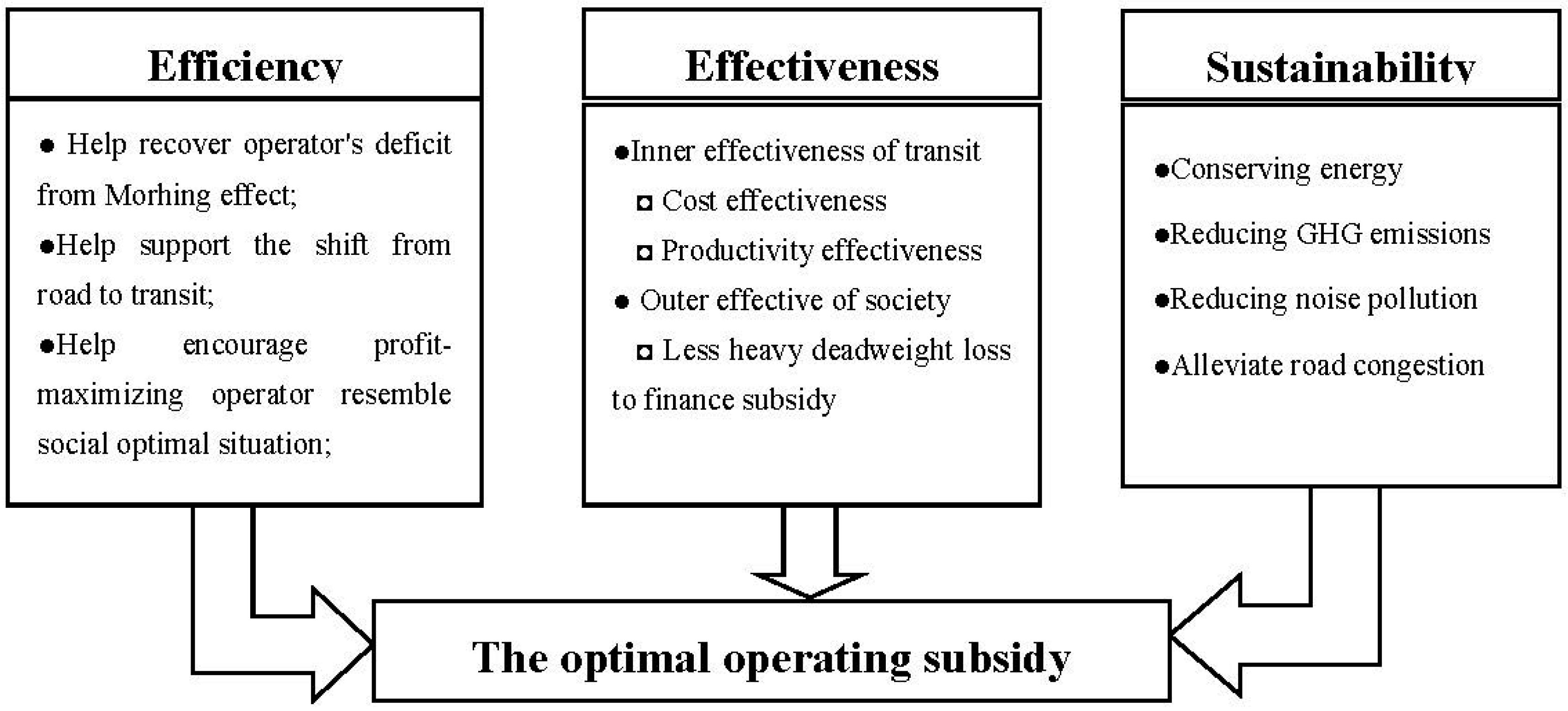
Although operating subsidy policies vary significantly between cities around the world, one general conclusion that can be drawn is that an optimal subsidy scheme should satisfy at least three key attributes, namely efficiency, effectiveness, and sustainability (See
Figure 1). The first attribute (
i.e., efficiency) emphasizes that the subsidy scheme should meet its intended objectives and help improve the well-being of all stakeholders. On the other hand, the second attribute—effectiveness is a measure of the output from subsidizing public transit that contributes towards improving social welfare with little deadweight loss to society. Finally, sustainability underpins the impact of subsidies from deterring residency from driving a car and shifting to sustainable public transport, which in turn help reduce GHG emissions, noise pollution, and eliminate severe road congestion.
Figure 1.
Three attributes of optimal operating subsidy scheme.
Figure 1.
Three attributes of optimal operating subsidy scheme.
Considering these three attributes, in practice, transportation planners have made great efforts to seek optimal subsidy schemes over the past decades. Up to now, although no definitive answer has been given in the general sense, some practical examples, in which efficient operating subsidies had been developed subject to actual circumstances, can be found across different countries. The first attempt to develop an optimal (or efficient) subsidy scheme that secures socially optimum behavioral responses from private operators was in Scandinavian countries. In the 1990s, Larsen, 1995 [
11] specifically designed an incentive-based subsidy scheme that could force the regulated monopolist—Oslo Public Transit Company—to resemble the situation of social welfare maximization. By updating and recalibrating Larsen’s model, Johansen
et al., 2001 [
12] and Fearnley
et al., 2004 [
13] proposed a remuneration scheme for private regulated transit companies, aiming to achieve the sustainability of the urban transport system. In contrast to Norwegian models, Hensher and his colleagues (Hensher and Prioni, 2002 [
14]; Hensher and Stanley, 2003 [
15]; Hensher and Wallis, 2005 [
16]) proposed performance-based quality contracts through a series of research works for Australian bus sector. Known as a patronage-based subsidy scheme, the subsidy rate per additional trip is linked to consumer surplus arising from the Mohring effect and the environmental and congestion externality benefits from mode switching. Similarly, focusing on a three-mode (bus, car, and subway) network, Parry and Small, 2009 [
17] analytically explored the optimal subsidies by accounting for several externalities, such as environmental externalities, in-vehicle crowding costs, road congestion, and accidents.
Building on previous analysis, this paper contributes to this strand of literature from two aspects. First, a two-stage game is formulated to investigate the social welfare-maximizing subsidy scheme and its impacts on a competitive urban transport market. Another feature that differentiates the present paper from previous studies is that it explicitly incorporates the external benefit of relieving road congestion and environmental externality into the proposed model.
3. The Optimal Subsidy Decision in a Competitive Transport Market
3.1. Basic Assumptions and Network Setting
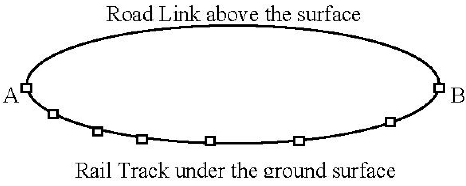
One urban traffic corridor with two links is used as a representation of one simplified urban transport network. As shown in
Figure 2, this traffic corridor is assumed to involve a rail transit line that operates on its own network and a surface road link that accommodates both buses and autos, which connects one original point A and one destination point B. In this mixed traffic case, buses and cars share road capacity so that the congestion externality has been caused by their interactions while in motion. However, the rail transit is running on an exclusive right-of-way with reliable schedules and definitely does not interact with buses and autos.
Figure 2.
A typical representation of urban traffic corridor with two links.
Figure 2.
A typical representation of urban traffic corridor with two links.
To abstract the essential ideas from the complicated real world, some simplifying assumptions are addressed:
Assumption 1: The urban transport system consists of three types of stakeholders, namely the local transport authority, public transport operators, and travelers. The local transport authority sets policy instruments to regulate and monitor a multi-modal transport system. Given these policy instruments, one bus company and one rail transit operator compete with each other in terms of fare levels and service frequencies. They do not collude, compensate each other, or maximize their joint profits. Observing attributes of each travel mode, travelers make their decisions on whether to travel and if so which mode to choose, based on travel utility maximization.
Assumption 2: To assess modal split behavior, one degenerate nested Logit model is adopted to model the market shares of alternative modes of transport. In the lower level (or public transit nest), as a potentially faster and more reliable mode, the rail transit is separated from conventional bus. While in the upper level, due to its spontaneous frequency, low access/egress times and highly personalized characteristics, auto travel is separated from public travel modes.
Assumption 3: All involved stakeholders have the most detailed knowledge, such as change in fare levels and service frequency, market demand and cost structures of transit services. Based on this perfect information, each agent can make rational decisions to fulfill his or her objectives.
Assumption 4: All travelers are homogeneous in terms of value of time.
3.2. The Specification of Demand, Cost and Subsidy Functions
The utility that one commuter perceives for travelling by automobile consists of monetary expenses (
), which include fuel, wear and tear on car usage together with parking and tolls if existent, and in-vehicle travelling time (
):
A (potential) traveler derives gross utility from taking one trip. Without loss of generality, this gross utility (denoted by
) can be normalized to zero.
denotes the constant value of in-vehicle travelling time. θ is a scale parameter to represent the variation of passenger perception on travel monetary expenses and time costs. The in-vehicle travel time (
TA) can be presented as a volume-delay function that developed by Bureau of Public Road (BPR):
In Equation (2), L is the length of the link and VA is the free-flow driving speed for cars. QA is the auto traffic flow and KA represents the capacity of the road. In the mixed traffic condition, the frequency of bus service (fb) is inserted into the BPR function to reflect this congestion interaction. γ is the passenger-car equivalent (PCE’s) of bus, which ranges from 1.5 to 3.
Moreover, the utility of choosing public transit services provided by rail transit or Bus Company can be expressed as:
where,
denotes the alternative-specific constant (ASC) for public transit, which reflects commuters’ preferences to bus or rail transit over the car.
is a flat fare charged by transit company.
stands for the average running speed of public transit. For frequent public transit services, if passengers arrive at stops in a random fashion without timing themselves according to the fixed schedule, the average passenger waiting time can be calculated as half of its headway (
).
denotes the constant value of waiting time.
Based on Assumption 2, a degenerate Nested Logit model is adopted to model the market shares of the alternative modes of transport. In this Nested Logit model, a choice at the public transit nest is more elastic than upper-level choices between private and public transport modes. Within the public transit nest, the market share associated with public transit service
i is:
where
is the conditional probability of choosing rail or bus given that the public transit is chosen. λ is the nesting coefficient ( or the dissimilarity parameter), which describes the degree of substitutability between bus and rail transit in the public transit nest. This scale parameter is bounded by zero and one (0 < λ < 1).
Then, the expected maximum utility (EMU) of public transit (
) can be mathematically expressed as:
At the upper level, the market share of travel mode
m (
m =
A,
T;
A = auto,
T = transit) is:
The total number of trips (
Q) along the urban corridor is assumed to be elastic with respect to the composite utility of travelling (denoted by
U):
Some studies assume the total demand to be inelastic. Obviously, this assumption may not be reasonable in reality since travelers’ decisions on whether to travel to some extent vary with the expected utility that the travelling can give. Hence, in this paper, the total demand in one urban commuting corridor is assumed to shrink or expand with a change in the composite disutility of travelling. To reflect this, a negative exponential function with respect to the composite utility (
U) is introduced, which is widely used in urban transport modeling (see Evans, 1992 [
18]; Williams
et al., 1993 [
19]):
where
Q0 is the total potential traffic demand in the urban traffic corridor during one particular period and ξ is the demand elasticity with respect to composite utility of travelling.
The demand function for transit services that operator
i affords is determined through substituting Equation (8) into Equations (6) and (11), which finally gives as:
The partial derivations of the public transit demand function (that is Equation (9)) with respect to price and frequency lead to:
We assume that the variable operating costs of transit service provisions are taken as a combination of unit cost of running vehicle-kilometers(
) and unit cost of taking on an additional passenger (
):
Furthermore, we assume the subsidy regime is tied to two service performances: trip-based subsidies ( per trip) and/or vehicle-kilometer-related subsidies ( per vehicle-kilometer).
To avoid large increases in subsidies and correspondingly excessive profits, a lump-sum payment () should be deducted from the total amount of subsidies, which would not alter operators’ strategic behaviors at the margin.
3.3. Two-Stage Game for Optimal Subsidy Decisions and Nash Equilibria
In a competitive urban transport market, the optimal selection of one subsidy scheme can be formulated as the following two-stage game. At the first stage, the public authority commits to a subsidy scheme that maximizes social welfare. Given the predetermined subsidy form and amount, the bus and rail transit operators compete with each other in terms of fares and frequencies in the second stage, which can subsequently cause the transport authority to update his decision leading to two transit operators’ reactions again. The interplay and interaction continue until a stable situation is reached, in which no stakeholder can improve his concerning objective function by changing his strategic variables. As usual, this two-stage game can be solved with standard backward approach.
The Nash equilibrium between the bus and rail transit competition at the second-stage is first sought by jointly solving the reaction functions with respect to price and service frequency. To derive these reaction functions, the meaningful objective of each operator is to maximize its own profit subject to capacity constraints. In the presence of subsidies, the operator’s profit, denoted by
πit, is made up of the fare-box revenue obtained from operating services, the costs associated with service provisions and the net subsidies granted by local transport authority.
subject to
where
is the vehicle capacity of public transit. Since the demand and cost functions are assumed to be monotonic and differentiable, it is easy to verify that each operator’s profit function is quasi-concave in the fare/frequency dimension, which in turn ensures the existence of a unique equilibrium.
To find the equilibrium price and frequency, we construct a Lagrangian function as:
The first order conditions of Equation (14) with respect to fare and frequency are given by:
Substituting Equation (10) into Equation (16) and rearranging the equation provides a solution for equilibrium price (denoted by
) in terms of the market share of public transit operator
i:
A closer look at the above mathematical expression for equilibrium fares indicates that in the absence of subsidy and capacity constraints (i.e., sp= sf = λi= 0), the equilibrium price is equal to the marginal passenger cost of transit service i () plus a mark-up, which relates to the market shares of public transit services. If there are a very large number of transit operators, the equilibrium price will be driven down to the first-best solution. In that extreme case, the equilibrium fare deviates little from the first-best solution. Subsidies (or tax) that direct link to vehicle-kilometers (or frequency) are sufficient to induce a profit-driven operator to approach first-best position. However, owing to the characteristic of transit services, the transit market is too thin to support too many operators. Thus, the common industry structure is duopoly competition. In the duopolistic case, the most probable result is that the prices are grossly above socially optimal (or first-best) levels, which substantially discourage public transport use and exacerbate the welfare losses from externality of automobile use. Owing to the substantial deviation between equilibrium fare and marginal social cost, oligopolistic operators should be subsidized based on ridership in order to drive down the competitive price.
When the capacity constraint is binding, the decision rule of equilibrium frequency is:
When the capacity constraint is not active, we substitute Equation (11) into Equation (17), which yields Nash equilibrium frequency (
):
Equation (20) shows that the equilibrium frequency increases with its own ridership (Qit), but decreases in the unit cost per departure (). Under an oligopolistic market structure, the competitive operators will increase their supply of the frequency in an effort to capture a bigger share of the available demand. As all operators do this, the overall frequency level probably increases. Thus, compared with the social welfare maximization output, whether the duopoly operator intends to undersupply or oversupply service frequency remains analytically undetermined.
At the first-stage, since the authority usually seeks a system-wide optimization, the appropriate objective for the transit authority to determine the operating subsidy is the maximization of social welfare From a perspective of a social planner, social welfare is the sum of consumer surplus, producer surplus, and externalities. The monetized GHG emission-type externalities can be calculated as
ψ represents the monetary cost per ton CO
2 equivalent. However, since the monetary value of this important parameter does not exist in China, we choose to not include GHG emission-type externality directly into social welfare function.
In the absence of the marginal cost of public funds, the subsidy is simply a transfer payment from the government to operators, which has no direct effect on social welfare as every dollar the government loses, the operator gains. In this sense, the only impact of this subsidy is via the changes in ridership that it generates. Unfortunately, the solutions of optimal subsidies cannot be explicitly expressed like the Nash equilibrium frequencies and fares.
Traditionally, the GHG emissions from vehicles can be calculated with two wide-spread modeling approaches: top-down (TD) models and bottom-up (BU) models (Nakata, 2004 [
20]). From a macro-economic perspective, a top-down approach (such as CGE, MACRO) mainly focuses on estimating aggregate relationships between the cost of emission producing activity and the level of GHG emissions, but usually ignores current and future technological options (Böhringer, 1998 [
21]). While, from a micro-technical point of view, a typical bottom-up approach (such as MARKAL, EFOM, LEAP) focuses on assessing the trends and financial costs of different technological options. Such models often neglect the macroeconomic impact of energy policies (Van Vuuren
et al., 2009 [
22]).
Concerning the availability of data and parameters, we adopt bottom-up approach (Wilson and Swisher, 1993 [
23]) in this paper to calculate the emissions of CO
2, CO, NO
X and CH:
EFni means the emission (tons) of pollutants n (i.e., CO2, CO, NOX and CH) from travel mode i during one year period. Qi means the number of traffic flow of travel mode i; VKTi is the average annual travel kilometers of car or bus; and EFni denotes the emission factor (g/Km) of pollutant n emitted from travel mode i. It should be noted, instead of using gasoline like car and bus, rail transit consumed electricity power which is mostly generated from coal power plants in the context of China. Thus the emission factor of pollutant n from rail transit need to be calibrated from electricity consumptions of running one rail-kilometer (Kw·h/rail-kilometer) and the level of pollutant n emitted from one kilowatt-hour electricity consumption.
4. The Computational Experiment
To approach the “realistic” urban traffic condition, an example network with 2012 Suzhou traffic data fits into the proposed two-stage game. Almost all chosen parameters are directly obtained or calibrated from the consulting reports, academic research, and the company’s accounting annual report, which were specifically made for the Suzhou area (See
Table 1).
Table 1.
Data and parameters for the computational experiment.
Table 1.
Data and parameters for the computational experiment.
| Symbols | Descriptions | Units | Values |
|---|
| Bus | Rail | Car |
|---|
| Vi | Average (or free-flow) travelling speed | kilometer/h | 20 | 40 | 50 |
| Kit | Capacity of the transit vehicles | Pass/vehicle | 120 | 960 | -- |
| KA | Capacity of the road | Cars/road | -- | -- | 7000 |
| Cost of taking on an additional passenger | CNY/passenger | 1.5 | 2 | -- |
| Marginal cost of providing transit service | CNY/veh-km | 8.9 | 22 | -- |
| βit | The alternative specific constant | - | −0.823 | −0.8098 | 0 |
| EFCO2 | Emission factor of CO2 | g/km | 904.72 | 574.22 | 125.6 |
| EFCO | Emission factor of CO | g/km | 10.83 | 2.55 | 4.13 |
| EFNOX, | Emission factor of NOx | g/km | 6.32 | 17.33 | 0.5 |
| EFCH | Emission factor of CH | g/km | 0.21 | 0.38 | 0.71 |
| L | The length of traffic corridor | km | 9 |
| θ | The scale parameter | - | 0.088 |
| λ | The nesting coefficient | - | 0.198 |
| ρw | The value of waiting time savings | CNY/h | 20.2 |
| ρv | The value of travelling time savings | CNY/h | 10.1 |
| ξ | Demand elasticity with respect to composite utility | - | 0.125 |
| γ | The passenger-car equivalent (PCE’s) | - | 1.5 |
To obtain model-specific traffic data and commuters’ mode choices, a joint RP&SP survey was conducted in the Suzhou metropolitan area in 2012. Survey respondents were chosen as Suzhou local residents who had commuted every day. First, those local residents are asked to represent their actual commutes (such as travel cost, travel time, number of transfers,
etc.) and socio-economic characteristics (such as age, gender, income, and education level,
etc.) in the form of a 24-hour travel diary (that is RP data). Afterwards, a SP survey designed to explore commuters’ tradeoff between alternative travelling cost and time is also applied to the same group that already interviewed in a previous RP survey. After testing consistency and validity of the resulting data, only commuters with an actual modal choice among car, bus, and train were considered, leading to a total of 6037 RP and SP observations available. Based on this survey, the average trip length of commuting trips in 2012 was around nine kilometers. According to current empirical experience, the free-flow travel speed is 50 km per hour for cars running on the arterial road. Simultaneously, this survey also suggests that the average running speed is 20 km per hour for buses and 40 km per hour for rail transit. The capacity of bus or rail is based on its physical capacity (
i.e., six people standing per square meter), leading to 120 passengers per articulated bus and 960 passengers per train. The operating cost functions for buses and trains are calibrated using the annual accounting report of bus and rail transit companies, which give the operating cost per passenger journey as 1.5 CNY for bus and 2 CNY for rail transit. The cost of running each vehicle-kilometer is 8.9 CNY for bus and 22 CNY for rail transit. The scale parameters in the degenerate nested Logit model (
i.e., θ = 0.088 and λ = 0.198) are in agreement with the empirically estimated values for mode choices in the Suzhou region [
24]. The values of emission factors from private cars and buses in the Suzhou area are recommended by the Suzhou Environment Protection Bureau.
To analyze the effects of operating subsidy on equilibrium outcomes, traffic flow of private cars, ridership of public transit and GHG emissions , three different subsidy schemes are proposed firstly, that is: (i) only trip-based subsidy scheme; (ii)only frequency-based (or vehicle-km-based) subsidy scheme; (iii) the joint implementation of trip-based and frequency-based subsidy schemes.
The data and parameters displayed in
Table 1 are used to solve the proposed two-stage game, assuming a potential demand rate is 7000 passengers per hour along this urban commuting corridor. The outcomes of this computational experiment are summarized in
Table 2 in terms of equilibrium fare, equilibrium frequency, and the magnitudes of optimal subsidies.
Table 2.
Optimal operating subsidies and Nash equilibrium solutions.
Table 2.
Optimal operating subsidies and Nash equilibrium solutions.
| | Reference Case | Scenario 1 | Scenario 2 | Scenario 3 |
|---|
| Variables | Social Optimum | Duopoly | Trip-Based | Frequency Based | Subsidy System |
|---|
| Control Variables |
|---|
| Bus fare (pb) | 1.5 | 3.495 | 1.144 | 3.544 | 1.145 |
| Rail fare (pr) | 2 | 4.450 | 2.202 | 4.406 | 2.198 |
| Bus frequency (fb) | 7.835 | 6.102 | 9.358 | 9.493 | 9.64 |
| Rail frequency (fr) | 8.866 | 5.401 | 8.17 | 6.218 | 8.26 |
| Trip-based subsidy (sp) | 0 | 0 | 2.522 | 0 | 2.425 |
| Frequency-related subsidy (sf) | 0 | 0 | 0 | 4.338 | 0.421 |
| Market Share and Demand Rate |
| Car market share (MA) | 60.29% | 80.83% | 60.46% | 78.65% | 60.26% |
| Transit market share (MT) | 39.71% | 19.17% | 39.54% | 21.35% | 39.74% |
| Car demand (QA) | 3236 | 3907 | 3242 | 3839 | 3235 |
| Transit demand (QT) | 2131 | 927 | 2120 | 1042 | 2133 |
| ►Bus demand (Qb) | 590 | 339 | 786 | 412 | 794 |
| ►Rail transit demand (Qr) | 1542 | 588 | 1334 | 630 | 1339 |
| Total transport demand (Q) | 5367 | 4834 | 5362 | 4881 | 5368 |
| Welfare Performance |
| Producer surplus (PS) | −2382 | 559 | 2759 | 981 | 2814 |
| ►Profit for bus (πb) | −627 | 188 | 876 | 453 | 908 |
| ►Profit for rail transit (πr) | −1755 | 371 | 1883 | 528 | 1906 |
| Total amount of subsidies (S) | 0 | 0 | 5347 | 614 | 5179 |
| Consumer Surplus (CS) | 42,935 | 38,667 | 42,893 | 39,046 | 42,942 |
| Social Welfare (SW) | 40,553 | 39,226 | 40,515 | 39,413 | 40,577 |
As a point of reference, we first calculate the social optimal case (Second column of
Table 2) and the duopoly competitive scenario (Third column of
Table 2), with which the outcomes of implementing alternative subsidy schemes can be assessed and compared. Being considered to be an ideal scenario, the social optimal case entails total deficits of 2382 CNY/hour for two transit operators with the marginal cost pricing (
i.e., 2 CNY for rail transit and 1.5 CNY for buses). Accordingly, the break-even operating subsidies amount to 41.4% of the operating costs for buses and 49.2% of the operating costs for rail transit. Another initial point of reference is the duopolistic competition in the absence of operating subsidies. In contrast to the social optimal case displayed, both transit operators make substantial profits, which are far more enough to cover their respective operating costs. However, for the given parameters and demand rate, one obvious and expected result is that the duopoly market is inferior to the welfare-maximizing monopoly market, as it leads to much higher fares (4.450 CNY for rail transit and 3.495 CNY for bus) and low service levels (5.4 trains per hour and 6.1 buses per hour). Thus, from an incentive perspective, the operating subsidy should be designed to induce the whole transport market toward social optimality.
Using the first-best case and duopoly case as a starting point, three proposed subsidy schemes have been tested to illustrate the role of subsidies in determining optimal and equilibrium outcomes, which leads to some interesting findings.
As expected, in the presence of subsidies, both transit operators respond by reducing fares and providing more services to satisfy the travel demand. Consequently, no matter what type of subsidy scheme is implemented, equilibrium fares are reduced and service frequencies are augmented. Compared with the duopoly case without any subsidies, the introduction of the trip-based subsidy leads to a sharp drop in fares (i.e., a decrease of 67.3% for buses and 50.5% for rail transit) and substantial improvements in service frequencies (i.e., an increase of 53.3% and 51.3% for buses and rail transit, respectively). Moreover, the frequency-related subsidy scheme stimulates improved services, although it only very slightly reduces fare equilibrium. In Scenario 3, the joint application of trip-based and frequency-related subsidy schemes essentially brings fares and frequencies pretty close to the socially optimal level. Consequently, a combination of transit improvements (fare reductions and frequency improvements) enables transit passengers to enjoy great increases in travel utilities.
For the chosen parameters, greater reductions in travelling disutility from taking bus or rail transit significantly influence the travel choice decisions of commuters, which in turn affect the demand levels of the three travel modes. In the case of the trip-based subsidy scheme (Scenario 1), total transit patronage is around 100% higher than total transit ridership in the case of the frequency-based subsidy scheme (Scenario 2). As noted from
Table 2, the implementation of operating subsidies makes public transit more attractive to commuters who were solely car users before. To this end, some previous car users shift their travel modes towards public transit, leading to a substantial reduction in the market share of car driving. Furthermore, a more detailed comparison of transit market share shows that the frequency-based subsidy scheme is preferable to bus operators, as it generates relatively larger market share (40%) than the other two subsidy schemes do (around 37%).
The concept of optimal subsidy in this study rests on the notion of producing the highest social welfare at the optimum. When each transit operator only receives a remuneration of 2.522 CNY for each additional trip (amounting to a total of 5347 CNY/h), social welfare reaches its highest level (40,515 CNY/h). In Scenario 2, the highest social welfare of 39,413 CNY/hour is obtained with a subsidy of 4.338 CNY for every vehicle-kilometer, costing 371 CNY per hour. For a given potential demand level, the social welfare improvement from merely implementing frequency-based subsidies is the smallest compared with the other subsidy schemes, indicating that Scenario 2 has a long way to approach the ideal scenario (first-best solution).
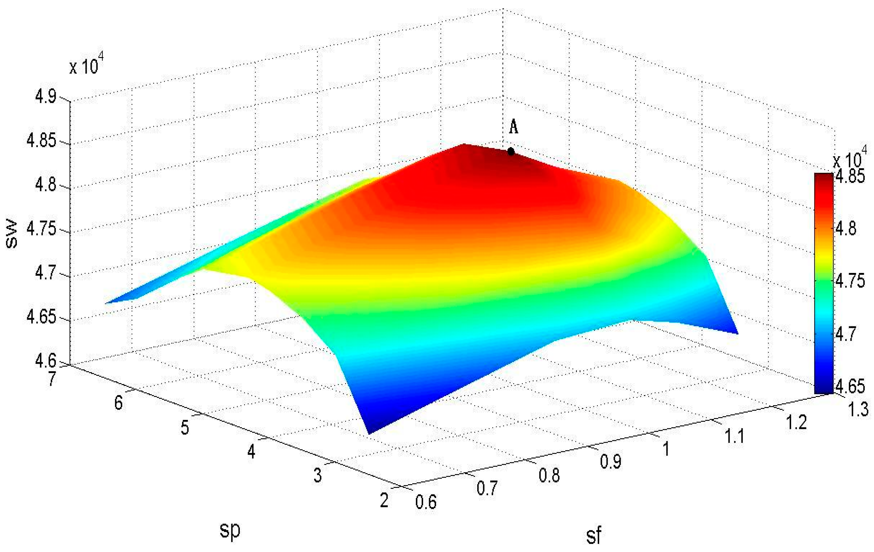
Figure 3 graphically shows the changes in social welfare with the combination of trip-based and frequency-based subsidy schemes (Scenario 3). Social welfare peaks at point A, at which 2.425 CNY is given for each additional trip and 0.421 CNY for each vehicle-kilometer. In total, the overall subsidy level amounts to 5179 CNY, divided between 1929 CNY for bus operators and 3250 CNY for rail transit operators. Compared with the trip-based subsidy scheme, the joint implementation of trip- and frequency-based subsidy schemes can achieve the highest welfare gains at a relatively low cost.
Figure 3.
The change in social welfare with the subsidy system.
Figure 3.
The change in social welfare with the subsidy system.
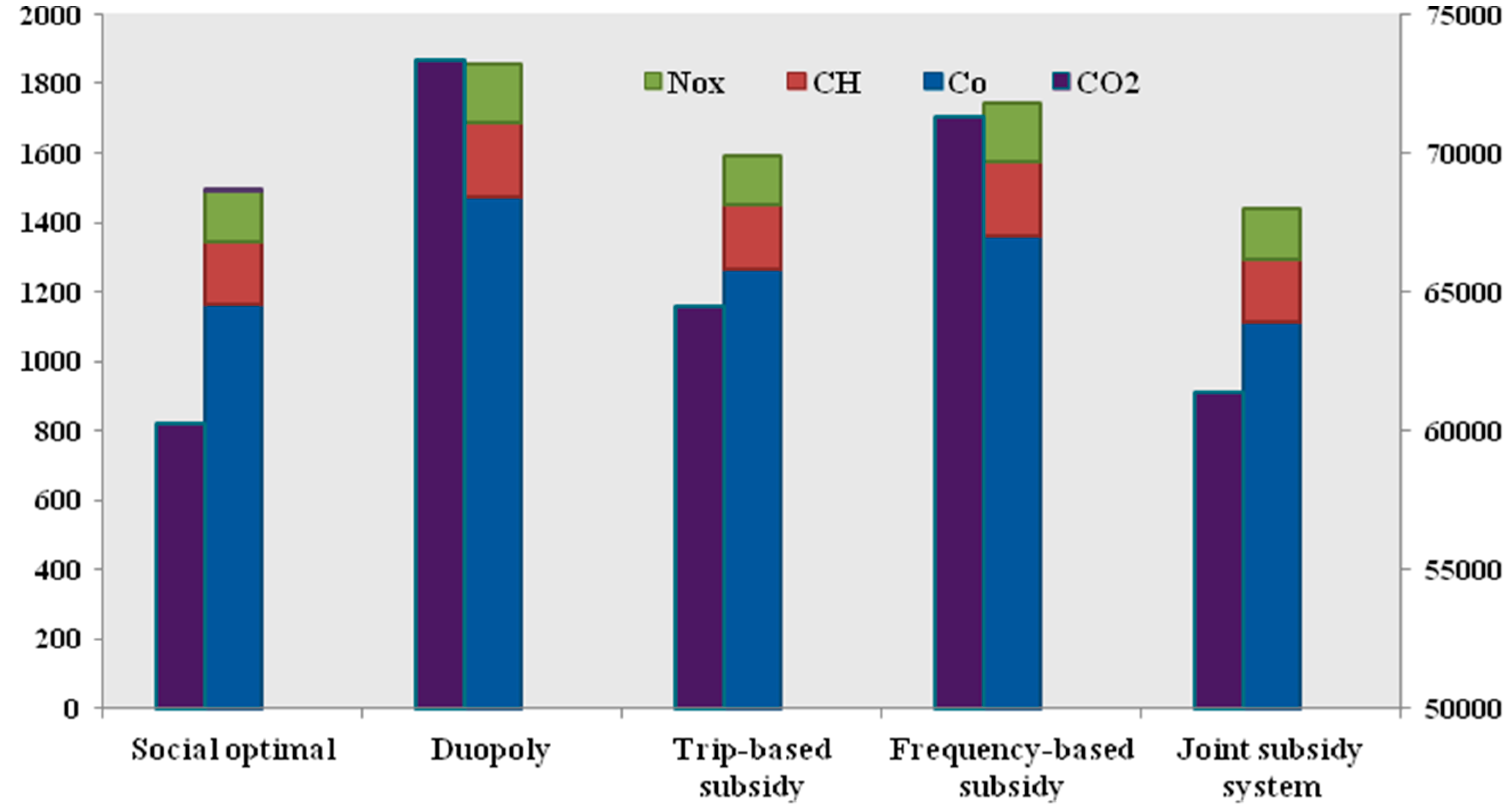
The last interesting result that can be summarized is related to the impact of optimal subsides on reducing GHG emissions. The effect of subsidizing public transit on reducing GHG emissions depends on many exogenous parameters, such as the cross elasticity between private and public transport modes, the degree of GHG emissions and the own elasticity of public transport. For the chosen parameters, three proposed subsidy schemes subsidizing public transit to some extent contribute to relieving GHG emissions, but their power to reduce GHG emission varies. As
Figure 4 depicts, compared to the duopolistic case, the joint implementation of trip-based and frequency-based subsidy scheme diminishes the CO
2 by 16.284%, CO by 24.25%, NO
X by 12.66%, and CH by 17.13% during one year period. It is obvious that jointly implementing the trip-based and frequency-based subsides can largely contribute to reducing all four types of greenhouse gas emissions, which nearly reach the social desired level.
Figure 4.
The Comparisons of GHG Emission Reduction.
Figure 4.
The Comparisons of GHG Emission Reduction.
5. Conclusions
Over recent decades, subsidies to urban public transport have become increasingly pervasive and important in both developed and developing countries. A well-targeted and well-designed subsidy scheme is clearly vital not only for transit passengers who must pay the charge and transit operators who receive monetary payment, but also for the users of alternative modes, such as car drivers.
This paper focuses on the design of optimum subsidy schemes in a competitive transport market to ensure that profit-maximizing operators coincide with social welfare objectives. To do this, a combination of one two-stage game and one degenerate nested Logit model is proposed, wherein the transit authority commits to a social welfare-maximizing subsidy scheme at the first stage and profit-maximizing operators compete on fares and frequencies at the subsequent stage. Analytical and empirical works for one two-link transport network are developed.
To illustrate the applicability of the proposed models, one numerical experiment for a realistic urban transport network is conducted using Suzhou traffic data. The main results of this paper can be summarized as follows. First, compared with socially optimal solutions, oligopoly competition generally results in higher fare, calling for the implication of trip-based subsidies. However, owing to uncertain competitive pressure, whether the non-cooperative duopoly operator aims to oversupply or undersupply is ambiguous. Consequently, a frequency-based subsidy or tax might be required to make a profit-driven operator offers the socially optimum frequency. Second, of the three proposed subsidy schemes, the joint implementation of trip-based and frequency-related subsidies not only generates the largest welfare gains but also makes competitive operators provide equilibrium fares and service frequencies, which largely resemble first-best optimal levels. Finally, the joint implementation of trip-based and frequency-based subsidies can largely contribute to reducing all four types of greenhouse gas emissions in the urban commuting corridor, which nearly reach the socially desired levels.
The proposed model has proven to perform well already, but further research is still needed to relax the strict assumptions made in this paper. For instance, it would be interesting to discriminate between subsidies instead of assuming that the bus industry receives the same subsidy level as rail transit does. It would also be worthwhile and realistic extending the two-link transport system to more complex transport networks. This generalization can be started with re-calibrating demand and cost functions by replacing the disaggregate data (such as frequency, number of passengers for single OD pair) that used in this paper with aggregate data (such as vehicle-kilometer, passenger-kilometer for multiple OD pairs) of whole transport network. Moreover, a large scale simulation models, such as VIPs and Visum, that handles all lines, OD pairs and modes simultaneously can be implemented to distribute commuters between routes within each public transport mode and between public transport modes and private car (For more comprehensive analysis of richer network structures in a monopoly transport market can be referred to Johansen
et al., 2001 [
12])
. Additionally, the present analysis has not considered the impact of marginal cost of public funds (MCF) on the determination of subsidies. In future work, these limitations might be overcome.


