A Linkage Model of Supply Chain Operation and Financial Performance for Economic Sustainability of Firm

Abstract

Although several studies have explored the relationship between the operation and performance of a supply chain (SC), a general SC model cannot deliver the expected financial results at a company-wide level. In this paper, we argue that this cannot guarantee the maximization of a firm’s overall value because short-term financial performance metrics do not reflect the risk to businesses and the invested capital. Owing to the varying natures of risk and the capital invested, firms with multiple divisions should assess each division separately, and the results can be compared for decisions concerning the allocation of the firm’s capital and resources to maximize the overall value of its businesses. We propose a linkage model to consider operational activities and financial performance simultaneously in a firm’s supply chain model. To exhibit the superiority of the proposed model that connects SC operation and financial indicators, we first compare the differences between models for maximizing profit and enterprise-wise economic value added (EVA) as objective functions. To examine uncertainty in the operational and financial parameters of the SC, the results of sensitivity analyses are then reported. Experimental results showed that our model, using the EVA approach, is more effective and superior in terms of maximizing the firm’s overall value from the long-term perspective while satisfying the target values for financial ratios set by the firm’s executives and shareholders for all periods, unlike the results of the general model.

1. Introduction

The concept of the supply chain (SC), which first appeared in the early 1990s, has been the focus of growing research interest, as the possibility of providing integrated supply chain management (SCM) can reduce the risk of unexpected/undesirable events throughout the network, and can markedly improve profit for all parties involved. Almost all SC optimization and modeling approaches address SCM problems in an isolated manner without analyzing the strengths or weaknesses of financial statements. SC managers generally deal with SC decision variables in order to solve problems by identifying the best arrangement of production facilities or distribution centers, the optimum flow of materials, and/or optimum position and levels of an inventory, and other common measures for profit maximization [1].

However, the top executives of a company, such as the chief executive officer (CEO), the chief financial officer, and the chief operation operating officer, tend to focus on such financial performance measures as sales, profits, stock price, and cost of capital [2]. Even though an important task of SC managers is to deliver the results of SC performance in terms of financial outcomes, they tend to concentrate on short-term operative improvements, such as profit or overall cost in SCM, and ignore the risk incurred and the capital invested by the firm.

Most research that deals with firm’s sustainability has emphasized the integration of three dimensions that represent economic, environmental, and social aspects [3,4].

Unlike previous studies, our research has focused on the economic sustainability in order to emphasize improving a firm’s financial performance and strengthening its soundness in the long-term. The term of economic sustainability named in this paper can be described as the systemic, strategic coordination of multiple business functions and tactics across business functions within a particular company for the purposes of improving the future financial performance of a particular firm and the supply chain as a whole. This means that firms that engage in sustainable supply chain attain higher financial performance in the long-term, unlike firms that concentrate on productivity and profitability over the short term.

Hence, to model a firm’s economic sustainability, long-term financial performance and a financial ratio to measure the soundness of the firm should be included. However, past studies focusing on operational aspects of traditional SC, which emphasize profitability, are fundamentally concerned only with profit-related issues, and lack a long-term strategic perspective [5,6,7].

Some researchers have tried to empirically test whether SC activities really affect the value of the firm and, if so, how much wealth is created through SC activities. They have designed conceptual frameworks to link SC activities with finance by using regression analyses and qualitative approaches such as in-depth interviews, surveys, and the Delphi methods.

On the other hand, this paper presents a mathematical model to link the operational and financial aspects. The model determines strategic decisions, such as hours of operation of facilities, as well as tactical decisions, such as quantities of production, inventory, and shipments, among network entities. Moreover, the model considers financial aspects by adding a set of budgetary constraints representing financial ratios. Moreover, the objective of the study is to maximize the sum of the economic value added (EVA) of each facility, instead of the traditional measure of profit in a holistic framework.

The remainder of the paper is structured as follows: In the next section, we review various studies that incorporate economic performances such as EVA, change in equity, and net present value (NPV) into a general supply chain. In Section 3, we discuss ways in which the SC operation model can be linked to financial indicators. Section 4 describes the proposed model to link SC drivers and financial performance by considering enterprise-wise SCM. We describe the application of our model in a case study in Section 5, and offer our conclusions in Section 6.

2. Literature Review

This study benefits from relevant studies that encompass financial aspects in the fields of operations and SCM. In this section, we provide a brief review of how financial performance is linked with the SC operational model.

Walters [8] first proposed a model to link EVA criteria and the logistics of operating management. His model identifies interrelationships between shareholder value planning and four strategic decision considerations: productivity, cash flow, profitability, and financial and investment management. Christopher and Ryals [9] examined the connections between SCM and the enhancement of shareholder value. They mainly addressed the four critical SC value drivers: revenue growth, operating cost reduction, the efficient use of fixed and working capital, and the generation of shareholder value. Douglas and Terrance [10] developed a framework to identify how suppliers and customers affect overall SC performance, and how supply chain metrics can be translated into shareholder value. Lambert and Burduroglu [11] reviewed six value measures in logistics and concluded that shareholder value measure is the best one of them. Pohlen and Goldsby [12] identified the difference between supplier-managed inventory and vendor-managed inventory, and combined them using EVA to represent the value-enhancement process. Hendricks and Singhal [13] estimated the impact of production and shipment delays on shareholder wealth and using an event study, concluded that delays have a negative effect on the stock on return.

Hendricks and Singhal [14] empirically tested whether SC disruptions have a negative impact on long-term stock prices and equity risk. In a similar manner, Hendricks and Singhal [15] showed that SC glitches damage performance. Chen et al. [16] investigated the inventories of US manufacturing firms between 1981 and 2000, and showed that firms with bad inventory management had poor long-term stock returns. Gunasekaran and Kobu [17] reviewed the literature on performance measures and metrics related to logistics and SC management. Johnson and Templar [18] developed a unified proxy to link SC and a firm’s value performance, and showed a positive relationship between SC efficiency and enterprise value using regression analysis. Ellinger et al. [19] used Delphi-style opinion data to show that top SC companies yielded higher operating performance in sales, cost, and working capital. Chang et al. [20] calculated meta-analytic mean correlations between SC indicators and various types of company performances. Their findings showed that the influence of internal integration on a firm’s performance become more significant over time. They emphasized the need for future research to further examine the complementarity of relationships among internal, supplier, and customer integration.

A few studies have dealt with decision models that maximize financial value using optimum SC variables. Guillen et al. [21] mentioned a conceptual strategy in enterprise management systems consisting of the integration of financial modeling with production plans and schedules. Through a comparison in a case study, the authors showed that the integrated approach yields further improvement by including scheduling models. Guillen et al. [22] proposed an integrated planning and budgeting model by inserting budgeting constraints that explored the financial ratios. In a case study, the authors showed that the integration model provides a better solution in terms of change in equity than the sequential approach that follows the hierarchical decision-making process. Hofmann and Locker [23] argued that the link between SCM and company value needs to be strengthened, since activities of the SC manager have a direct impact on stakeholders. Badri et al. [24] designed a scenario-based stochastic optimization model to maximize the value of the company by maximizing EVA. To generate continuous random variables in designing scenarios, the Nataf transformation was applied.

Cardoso et al. [25] designed a mixed-integer linear programming model to maximize the expected NPV of SC and minimize financial risk. They considered four types of financial risk: the difference between the expected NPV and the NPV value of a given scenario, penalization according to lower-than-expected value, downside deviation from a given target for an expected NPV, and the risk of being lower than the conditional value-at-risk. Most other studies have either focused on improving short-term financial performance or have disregarded financial decision-making processes altogether, which cannot guarantee value enhancement for firms. In order to overcome the limitations of previous studies, in this study, we propose a conceptual framework for a supply chain finance model for firm-value maximization that links financial measures and SC activities and provides a case study for application through our simplified mathematical model.

Gaur et al. [26] proposed an integrated optimization model for a closed-loop supply chain to maximize the NPV of total net profit over the entire lifecycle of both new and reconditioned products while satisfying financial constraints relevant to a closed-loop supply chain. Based on a real-world case study of a battery manufacturer, the experimental results of their study showed that using NPV as objective function is significantly better than the general supply chain model. Ramezani et al. [27] confirmed that using NPV is effective in designing a logistics network with the fuzzy-based integer programming.

Tognetti et al. [28] proposed an integration model that is consistent with environmental standards and concern for profitability. To handle its environmental and economic objectives, they measured economic performance using the NPV of variable costs and environmental impacts through CO₂-equivalent emissions based on the lifecycle assessment methodology.

Ramezani et al. [29] presented integrating the financial and physical flows of closed-loop supply chains in designing a bi-objective logistic network reflecting the uncertainty in demand and return rate using long-term possible scenarios. The results compared in terms of the change in equity for different scenarios and the effectiveness in the financial models confirmed that incorporating financial models leads to higher overall earnings and insights into interactions between operations and finances.

Ramezani et al. [30] introduced a method to incorporate the financial aspects (i.e., current and fixed assets and liabilities) into a set of constraints relevant to the budget through balances of cash, debt, securities, payment delays, and discounts in supply chain planning. To show the advantage of using the financial model, the financial approach and traditional approach were compared. The results of their study indicated that the traditional model leads to lower change in equity than the financial model.

3. Ways to Link SC Operations and Financial Performance

3.1. Link among Financial Objectives in Supply Chain Operation

Profit maximization is generally considered the major objective of SC operation modeling. However, the use of such an objective as the profit maximization (or minimization of total cost) has some limitations. The term “profit” is vague when considering financial indicators. Profit can be net profit, gross profit, after-tax profit, or the rate of profit. There is thus no clear definition of profit maximization. The idea even ignores time value of money. The total profit used as an objective function in SCM is surely an important decision variable. However, it is meaningful only if it reflects the time value of money. Another limitation of profit maximization is that it ignores financial risk to the business. If the risk is ignored, the firm’s sustainability that evaluates its soundness in the long term can be called into question. Profit maximization also neglects intangible benefits, such as quality, brand power, and technological advancements, which can be core SC value drivers. The addition of intangible assets contributes to value creation for SC objectives. They indirectly, and sometimes directly, create financial value for the company.

The ultimate goal of a corporation is to maximize the wealth of shareholders, assuming that the financial markets are efficient. As mentioned in the previous section, a few researchers have attempted to connect SC value drivers with financial measures. The financial metrics mainly used in the relevant studies dealt with accounting variables, such as earnings or return on investment. As with profit maximization in a generic SC model, the use of accounting variables as performance metrics ignores the cost of capital, which reflects the risk to businesses. Moreover, accounting metrics are not a cash-flow metric, which can be crucial in financial valuation. Even if the firm achieves outstanding accounting profits, it is possible for it to go bankrupt if it does not have actual cash on hand. Owing to these drawbacks in the use of accounting metrics, researchers have begun using risk-adjusted cash flow variables as financial metrics, such as free cash flow of firm (FCFF) and EVA, developed and trademarked by Stern Stewart & Company (Munich, Germany) [31].

EVA has the advantage that it is simple to calculate and easy to understand. However, EVA has not been properly used in current SC research because it often ignores the time value of money. Firm value maximization is identical to maximizing the present value (PV) of EVA over time. This implies that firm value maximization through EVA is only assured if the firm maximizes the PV of future EVAs.

If the time value of money is ignored, it is possible for managers to make value-destroying decisions by focusing on present improvements in EVA at the cost of future EVA [32]. Sacrificing future EVA means that managers can increase the EVA at the time by delaying capital expenditure, like reducing research and development investment. 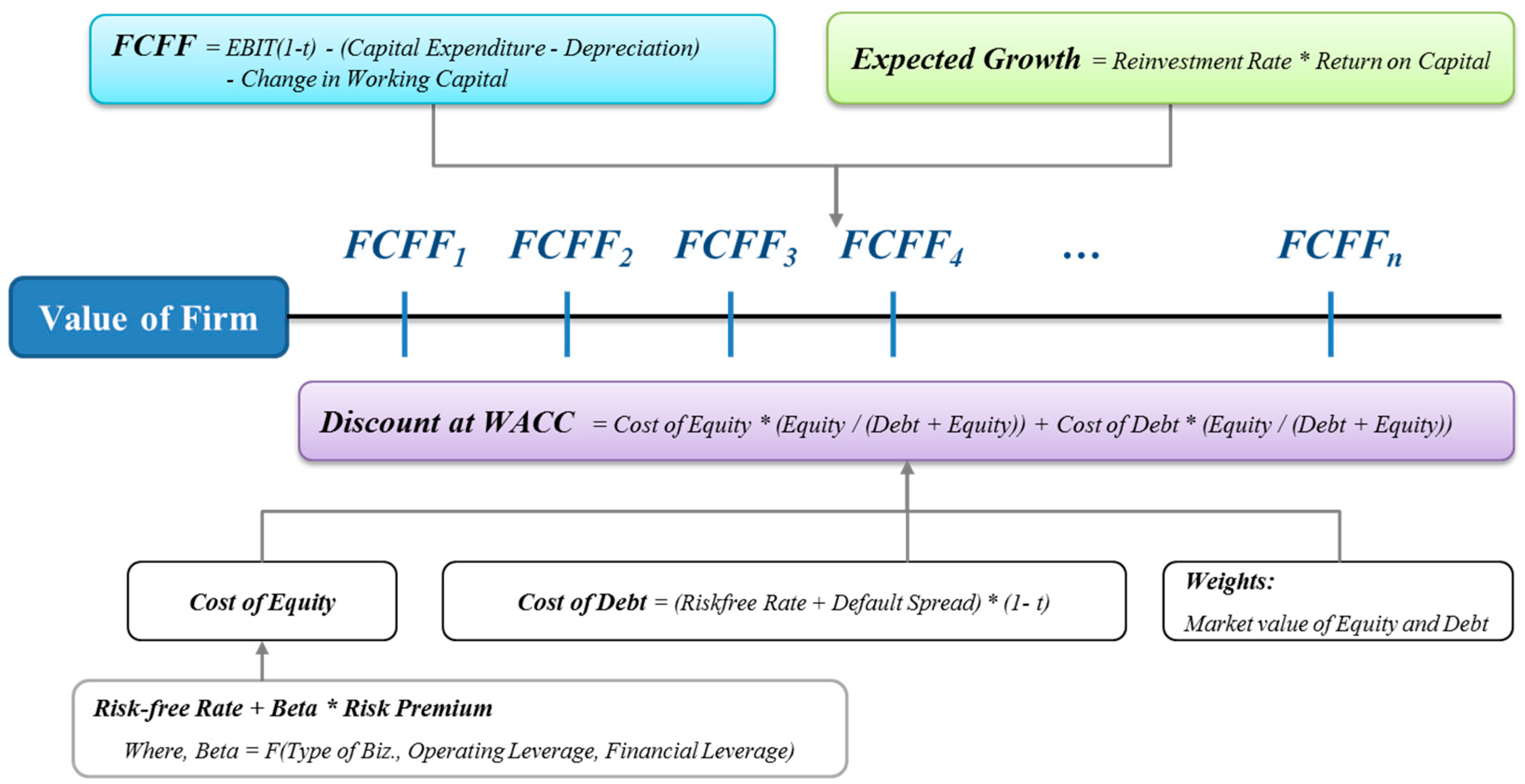Start-ups and high-growth firms need large capital expenditures or reinvestment, which results in negative EVA [33]. However, negative EVA at a given time does not mean the firm’s value has decreased, and can indicate its future growth prospects. Past models that use EVA as performance metric focused on improving the given EVA, which may not coincide with firm value maximization. Therefore, financial performance metrics should be considered as the PV of future EVA or cash flows over time. Another important point in applying financial metrics to SC performance is that the firm’s resources and capital are limited. Divisions within a firm compete for resources and capital. Thus, the firm’s executives should effectively allocate resources. Nevertheless, past models often ignored the financial decision-making process in a firm. We use a discounted cash flow approach to measure the value of the firm, which reflects the hierarchical process involving financial decisions by executives and SC decisions, in Figure 1 [34].

Figure 1. Valuing a firm. FCFF: free cash flow of firm; EBIT: earnings before interest and taxes; WACC: weighted-average cost of capital.

3.2. The Framework of the Linkage Model

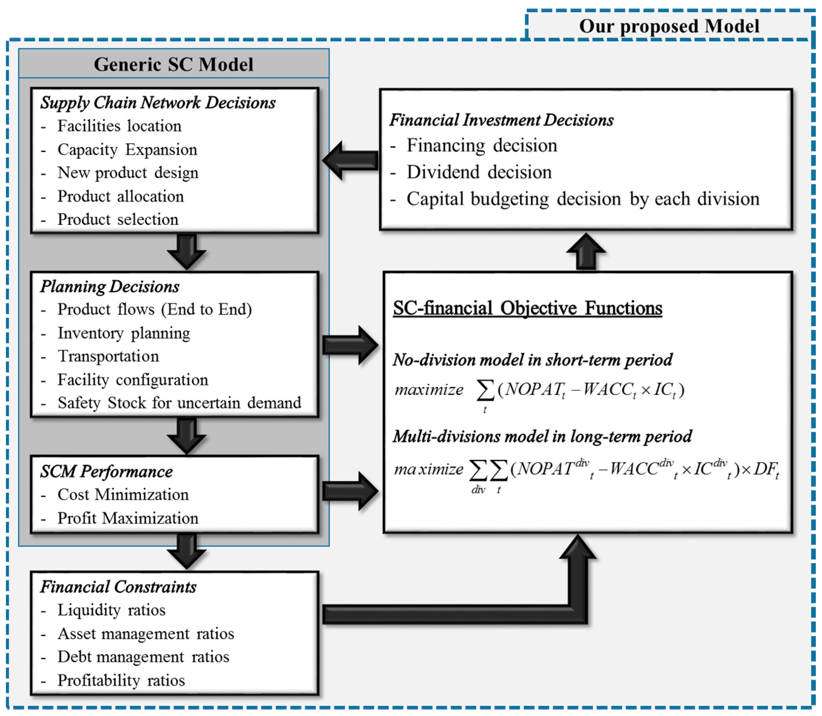
The house integration model for the link between SC operations and firm value drivers is shown in detail in Figure 2. A firm’s value can be determined by investment, financing, and decisions concerning dividends made by top executives. The roof rests on two pillars representing the two main components of firm value drivers: financial objectives and financial performance indicators. Firm value drivers are broken down into their building blocks, representing SC value performance. The three foundations represent SC value drivers.

Figure 2. House-of-integration model for the link between supply chain (SC) operations and firm value.

Large firms typically have several divisions (segments) that produce different types of products with their own SC network flows. Since demands, cost, and sales are different for each product, risk is different as well (divisional financial information, such as sales, cost, and inventory, are available through annual reports). When evaluating SC activities that require the investment of large amounts of capital, top executives should understand the risk posed by each division. Suppose that a firm has two divisions (A and B), where each is in a different industrial sector and produces various types of products. The managers of each division expect to obtain the most of the firm’s resources and capital in order to improve the financial performance of their division because their compensation is tied to divisional performance. It is certain that each division has a unique cash flow stream, and is thus exposed to different risk factors. In other words, each division has its own return and risk. Suppose further that for division A, the products are sold steadily regardless of market conditions; division B has massive potential to grow, but has a high chance of failure. Since division A has stable sales, it does not pose much risk, but the expected return on investment is low. On the other hand, division B has significant potential, but bears risk of failure.

Suppose each division has proposed an SC project to expand its warehouse and distribution capacities, and so on. Division A, with low risk, has low cost of capital but low expected return as well. Division B, however, has higher cost of capital but higher expected return than division A. The divisional managers approach top executives in order to obtain funds for their SC projects. If the executives use weighted-average cost of capital (WACC) to assess each project, division A’s project is rejected and division B’s project is accepted. If this continues, most of the firm’s capital resources will be allocated to division B. The correct decision by top executives in this case is that the return and the risk offered by the divisional projects should be evaluated separately by using each division’s own numbers. Another advantage of divisional analysis is that firms often have capital rationing. Firms set limits on their investments, even if they have valuable new SC projects, based on a capital rationing policy. This is imposed either internally or forced by market conditions. In capital rationing, firm’s best decision is to choose the most profitable (highest EVA (or NPV)) project relative to the size of investment, given its total budget.

Thus, firms with multiple divisions should pay attention to the proper allocation of capital and resources given the financial status of each division. Furthermore, given budgetary constraints, each division should adjust its SC strategies to achieve its SC objectives accordingly.

3.3. Decision-Making Procedure in Linkage Model

Figure 3 shows details of SCs and financial decision-making procedures of our model with seven steps. In practice, enterprise-wise financial and SC decisions are determined by combining the bottom-up and top-down procedures over time. It is typical for a firm to have an operation plan for five years or more in its planning horizon. Thus, this plan linking enterprise-wise financial and SC decisions includes a strategy for how capital and resources are allocated, sets up deadlines for specific task, and sets targets for growth, sales, and profit, among others. Therefore, we propose a model that links the decision process and SC activities at each of strategic, tactical, and operation levels, and shows how decisions made at each level affect those in the others in seven sequential and circular processes.

Figure 3. Proposed models for the decision process of firm value maximization.

(1)

Operational SC decision: The first step of our model involves defining what SC drivers mean and analyzing how they affect financial ratios (e.g., inventory turnover, days sales outstanding, profit margin, and more) of SC objectives, such as profit maximization and its growth. The results of ratio analyses are delivered to the managers of business units.

(2)

Tactical SC decision: Financial and SC data delivered from operational levels are gathered and analyzed in this step. The managers of business units (or product groups) evaluate SC performance and financial ratios based on target values planned previously. They also monitor the trends of each performance measure to find strong/weak points of SC activities at the time. Based on the analyzed data, the managers of the business units set up the SC tactical plan for activities such as purchasing, production volume, inventory policy, and transport strategies, as shown in Figure 3. Information containing performance results at the time and the next period’s tactical plan for SC operations are then delivered to the managers of each division.

(3)

Strategic SC decision: Divisional managers need to classify strong business units and under-performing ones based on firm value drivers, such as free cash flow, growth rate, cost of capital, and length of growth period. They then determine overall SC strategies, such as SC network configuration and design of embedded facilities. This process allows division managers to set the target growth rate and the capital (additional fund) budget for business units for the next decision period. Division managers prepare aggregated firm value drivers for the given period and the next one to submit to top executives.

(4)

Enterprise-wise decision: Top executives first analyze the given and future firm value drivers of each division, and devise strategic plans that form the basis of long-term planning. In order to make investment, financing, and dividend decisions at the same time, the firm constructs projected financial statements by considering future levels of sales, costs, and interest rates, and sets target ratios. Based on these, decisions are made about how capital and resources are allocated among divisions, which is known as the capital budgeting process. In this process, the initial plan is modified according to its target ratios and adjusted in a way that maximizes the value of the firm. The adjusted operating plan is returned to each division manager.

(5)

Adjustment of strategic SC decision: Each division examines potential gaps in the next period’s plan in the new capital budget, and builds a revised plan that incorporates the target growth rate for and the capital budget needed by each business unit. He/She also needs to prepare a modified plan for the SC network. The adjusted strategic SC decision is handed down to business units.

(6)

Adjustment of tactical SC decision: Business units adapt tactical SC decisions, which include purchasing/production volumes, proper inventory policy, and transportation strategies, in light of budgetary constraints and the redesigned SC structure.

(7)

Adjustment of operational SC decision: Finally, the SC managers of business units, based on the adjusted strategic and tactical decisions, operate the SC after identifying core SC value drivers, or making decisions on the weight of each value driver satisfying SC objectives.

4. Analytical Approach to Linkage Model

4.1. Overview of Analytical Linkage Model

We represent the connection between financial and SC operations in an SC network with a simplified mathematical formula. The SC operation model proposed in this example has been extended in studies by Longinidis and Georgiadis [35,36] to describe an integrated, division-based operation model. This model divides the constraints into four: inventory mass balance equations, constraints related to warehouse and distribution center capacity, safety stock and logical constraints of transportation flow, and equations linking the financial model and the constraints. The financial model aims at finding the expected corporate value, which is the objective function to be maximized. A few financial constraints are also included to solve our model, such as liquidity ratios, asset management ratios, debt management ratios, and profitability ratios. Liquidity ratios measure the short-term ability to pay debt obligations. It consists of the current ratio, the quick ratio, and the cash ratio. Each liquidity ratio can be expressed as following equations.

Liquidity ratios are closely connected with the cash management of the SC.

• Current ratio = Current asset/Current liabilities
• Quick ratio = (Current asset − inventory)/Current liabilities
• Cash ratio = Cash and equivalents/Current liabilities

Asset management ratios measure how effectively a firm manages its assets. It consists of a receivables turnover ratio and a fixed-assets turnover ratio. The first measures how a firm is managing assets other than cash at a given time, and the second measures the efficiency of fixed assets.

• Receivables turnover ratio = Sales/Receivables
• Fixed assets turnover ratio = Sales/Fixed assets

On the other side of the balance sheet in financial statements are debt management ratios. They measure how much debt a firm has and its ability to pay interest on it. The first debt management ratio is the total debt ratio, which can be easily converted into debt-to-equity ratio. The other ratios are long-term debt ratio and cash coverage ratio.

• Total debt ratio = Total Debts/Total assets
• Debt to Equity = Debt/Common equity
• Long-term debt ratio = Long-term liabilities/(Long-term liabilities + Common equity)
• Cash coverage ratio = (Earnings before interest and tax + Depreciation)/Interest expenses

Finally, there are profitability ratios that show the net effects of the liquidity, the asset management, and the debt management ratios. The ratios consist of profit margin, return on assets, and return on equity. These ratios measure how profitable the business is, and how much a firm can return to investors, shareholders, and debt holders.

• Profit margin = Net income/Sales
• Return on assets = Net income/Total assets
• Return on equity = Net income/Common equity

As shown in Figure 4, we use all the ratios mentioned above as financial constraints to check the impact of financial constraints on supply chain decisions in addition to different objective functions.

Figure 4. The link between SC operation and financial models. SCM: supply chain management; NOPAT: net operating profit after tax; IC: invested capital; DF: discount factor.

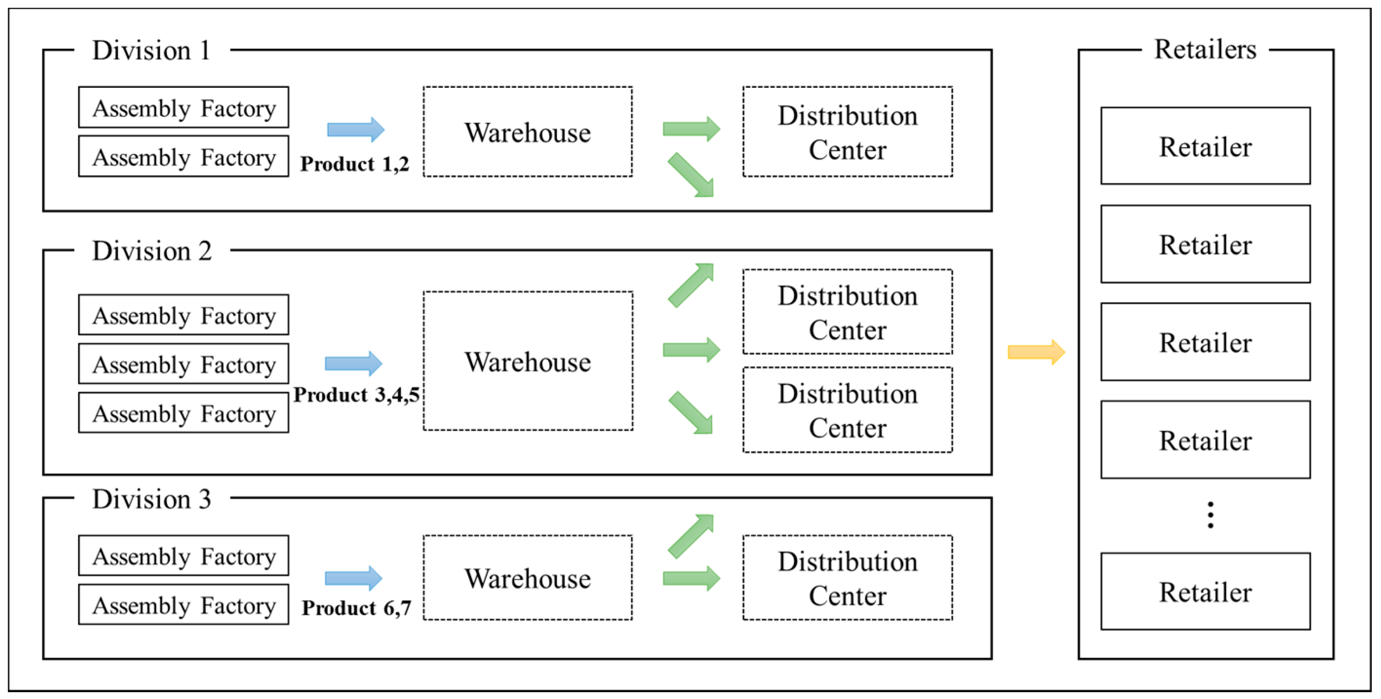
To implement our case study, we designed an SC network consisting of three assembly factories to produce two or three different products with raw materials, a single warehouse by division, and four distribution centers shared among the divisions, as shown in Figure 5.

Figure 5. SC network considered in this example.

Prior to describing the model in Section 4.2, we introduce basic assumptions and limitation of our model as below:

• The location of assembly factories, warehouses, distribution centers, and retailers are known and fixed.
• The flow is only permitted to be shipped between two consecutive stages. Moreover, there are no flows between facilities in the same layer.
• The quantities of all parameters are deterministic.
• The capacities of facilities are sufficient to satisfy all demands at all periods.
• Storage cost is calculated by the average inventory of two consecutive periods.

4.2. Mathematical Model

The proposed model considers both SC operation and financial decisions in the SC. Mixed-integer linear programming was used to solve the SC network containing multiple echelons, multiple products, and multiple periods of the SC.

Notations

Indices

$p$	Product
$e$	Production equipment
$f$	Assembly factory (A.F)
$w$	Warehouse (W.H)
$d$	Distribution center (D.C)
$r$	Retailer (=deployment partner)
$t$	Time period
$div$	Division

Sets

$P{F}^{set}$	Set of products belonging to the specific A.F
$P{W}^{set}$	Set of products belonging to the specific W.H
$F{W}^{set}$	Set of assembly factories belonging to the specific W.H
$PDI{V}^{set}$	Set of products belonging to the specific division
$FDI{V}^{set}$	Set of assembly factories belonging to the specific division
$WDI{V}^{set}$	Set of warehouses belonging to the specific division
$DDI{V}^{set}$	Set of distributions center belonging to the specific division

Parameters

$cap{a}_{pf}^{max}$	Maximum production capacity of A.F f for product p
$cap{a}_w^{max}$	Maximum capacity of W.H w
$cap{a}_d^{max}$	Maximum capacity of D.C d
$cap{a}_{pf}^{min}$	Minimum production capacity of A.F f for product p
$cap{a}_w^{min}$	Minimum capacity of W.H w
$cap{a}_d^{min}$	Minimum capacity of D.C d
$cos{t}_{pf}^{AF}$	Unit assembly cost of product p at A.F f
$cos{t}_{pw}^W$	Unit handling cost of product p at W.H w
$cos{t}_{pd}^D$	Unit handling cost of product p at D.C d
$cos{t}_{pf}^I$	Unit inventory cost of product p at A.F f
$cos{t}_{pw}^I$	Unit inventory cost of product p at W.H w
$cos{t}_{pd}^I$	Unit inventory cost of product p at D.C d
$cos{t}_w^{fix}$	Fixed cost of establishing W.H w
$cos{t}_d^{fix}$	Fixed cost of establishing D.C d
$cos{t}_{pfw}^{TR}$	Unit transportation cost of product p transferred from A.F f to W.H w
$cos{t}_{pwd}^{TR}$	Unit transportation cost of product p transferred from W.H w to D.C d
$cos{t}_{pdr}^{TR}$	Unit transportation cost of product p transferred from D.C d to retailer r
$deman{d}_{prt}$	Demand for product p from retailer r during period t
$i_{pft}^{min}$	Minimum inventory of product p in A.F f during period t
$i_{pwt}^{min}$	Minimum inventory of product p in W.H w during period t
$i_{pdt}^{min}$	Minimum inventory of product p in D.C d during period t
$pric{e}_{prt}$	Price for product p for retailer r during period t
$q_{fw}^{max}$	Maximum rate of flow from A.F f to W.H w
$q_{wdd}^{max}$	Maximum rate of flow from W.H w to D.C d
$q_{dr}^{max}$	Maximum rate of flow from D.C d to retailer r
$q_{fw}^{min}$	Minimum rate of flow from A.F f to W.H w
$q_{wd}^{min}$	Minimum rate of flow from W.H w to D.C d
$q_{dr}^{min}$	Minimum rate of flow from D.C d to retailer r
$r_{fe}$	Total rate of availability of equipment e at A.F f
$cc{r}_t$	Minimum bound for cash coverage ratio at the end of time period t
$ni{p}_t$	Percent of net income connected to cash flow at the end of time period t
$c{r}_t$	Minimum bound for current ratio at the end of time period t
$cu{r}_t$	Minimum bound for current ratio at the end of time period t
$de{r}_t$	Upper bound for debt equity ratio at the end of time period t
$d{f}_t^{div}$	Discount factor at the end of time period t for each division div
$d{r}_t$	Depreciation ratio at the end of time period t
$fat{r}_t$	Lower bound for fixed asset turnover ratio at the end of time period t
$ltd{r}_t$	Upper bound for long-term debt ratio at the end of time period t
$lt{r}_t$	Long-term interest rate at the end of time period t
$pm{r}_t$	Lower bound for profit margin ratio at the end of time period t
$q{r}_t$	Lower bound for quick ratio at the end of time period t
$roa{r}_t$	Lower bound for return on asset ratio at the end of time period t
$roe{r}_t$	Lower bound for return on equity at the end of time period t
$rt{r}_t$	Lower bound for receivable turnover ratio at the end of time period t
$st{r}_t$	Short-term interest rate at the end of time period t
$td{r}_t$	Upper bound for total debt ratio rate at the end of time period t
$t{r}_t$	Tax rate at the end of time period t
$wac{c}_t^{div}$	Weighted-average cost of capital at the end of time period t by each division div
${\gamma }_{pw}$	Coefficient relating capacity of W.H w to inventory of product p held
${\gamma }_{pd}$	Coefficient relating capacity of D.C d to inventory of product p held
${\rho }_{pfe}$	Coefficient of rate of use of equipment e in A.F f to produce product p

Decision Variables

$C_t^{div}$	Cash at the end of time period t for each division div
$C{A}_t^{div}$	Assets at the end of time period t of each division div
$C{D}_{dt}$	Capacity of D.C d during time period t
$COG{S}_t^{div}$	Cost of goods sold at the end of time period t by each division div
$C{W}_{wt}$	Capacity of W.H w during time period t
$DP{R}_t^{div}$	Depreciation at the end of time period t by each division div
$E_t^{div}$	Equity at the end of time period t of each division div
$EBI{T}_t^{div}$	Earnings before interests and tax at the end of time period t of each division div
$F{A}_t^{div}$	Fixed asset at the end of time period t of each division div
$FA{I}_t^{div}$	Fixed asset investment of each division div
$H{C}_t^{div}$	Handling cost at the end of time period t for each division div
$I_{pft}$	Inventory level of product p at A.F f at the end of time period t
$I_{pwt}$	Inventory level of product p at W.H w at the end of time period t
$I_{pdt}$	Inventory level of product p at D.C d at the end of time period t
$I{C}_t$	Invested capital at the end of time period t by each division div
$IN{R}_t^{div}$	Value of inventory at the end of time period t of each division div
$I{P}_t^{div}$	Interest paid at the end of time period t by each division div
$LT{L}_t^{div}$	Long-term liabilities at the end of time period t of each division div
$N{C}_t^{div}$	New cash during the time period t for each division div
$N{E}_t^{div}$	New equity during the time period t for each division div
$N{I}_t^{div}$	Net income at the end of time period t of each division div
$NI{S}_t^{div}$	New issued stocks at the end of time period t of each division div
$NOPA{T}_t^{div}$	Net operating profit after taxes at the end of time period t of each division div
$NR{A}_t^{div}$	New receivable during time period t by each division div
$NT{S}_t^{div}$	Total sales at the end of time period t of each division div
$P_{pft}$	Production rate of product p in A.F f during time period t
$P{C}_t^{div}$	Production cost during time period t by each division div
$R{A}_t^{div}$	Receivable accounts at the end of time period t of each division div
$Q_{pfwt}$	Rate of flow of product p from A.F f to W.H w during time period t
$Q_{pwdt}$	Rate of flow of product p from W.H w to D.C d during time period t
$Q_{pdrt}$	Rate of flow of product p from D.C d to retailer r during time period t
$S{C}_t^{div}$	Storage cost during time period t by each division div
$ST{L}_t^{div}$	Short-term liabilities at the end of time period t of each division div
$T{C}_t^{div}$	Transportation cost during the time period t for each division div
$T{I}_t^{div}$	Taxable income at the end of time period t of each division div
$Z_{wt}$	1 if W.H w is to be established at time period t and it will be opened for all periods later, 0 otherwise
$Z_{dt}$	1 if D.C d is to be established at time period t and it will be opened for all periods later, 0 otherwise
$PW{D}_{wdt}$	1 if product is to be transported from W.H w to D.C d during time period t, 0 otherwise
$PD{R}_{drt}$	1 if product is to be transported from D.C d to retailer r during time period t, 0 otherwise

Objective function

The objective function of the proposed model is intended to maximize the EVA of the firm over the time periods. It is computed to sum up the EVA of each division, calculated by the net operating profit after tax (NOPAT), in period t minus the total cost of invested capital in the net operating assets at the end of the previous period, adjusted by the weighted-average cost of capital. Equation (1) represents the objective function that maximizes EVA:

$$maximize{\displaystyle \sum _{t,div}\left(NOPA{T}_t^{div}-wac{c}_t^{div}I{C}_t^{div}\right)}\times d{f}_t^{div}$$

(1)

Equations (2) to (25) show constraints on SC operation, and Equations (26) to (47) are financial constraints. Equations (48) to (59) explain the constraints on financial ratios indicating the financial soundness and efficiency of a firm.

Equations (2) and (3) show the binary constraints to decide whether each facility, including warehouses and the DC, is open, and Equations (4) to (6) guarantee that only open facilities can receive or send products:

$${\displaystyle \sum _{\tau =1}^t{Z}_{w\tau }}\le 1\forall w,t$$

(2)

$${\displaystyle \sum _{\tau =1}^t{Z}_{d\tau }}\le 1\forall d,t$$

(3)

$$PW{D}_{wdt}\le {\displaystyle \sum _{\tau =1}^t{Z}_{w\tau }}\forall w,d,t$$

(4)

$$PW{D}_{wdt}\le {\displaystyle \sum _{\tau =1}^t{Z}_{d\tau }}\forall w,d,t$$

(5)

$$PD{R}_{drt}\le {\displaystyle \sum _{\tau =1}^t{Z}_{d\tau }}\forall d,r,t$$

(6)

Equations (7) to (12) show that for each facility open in period t, the goods’ flow should be between the minimum and maximum capacities of each facility.

$${\displaystyle \sum _{p\in P{F}^{set}}{Q}_{pfwt}}\le q_{fw}^{\max }{\displaystyle \sum _{\tau =1}^t{Z}_{w\tau }}\forall f\in F{W}^{set},w,t$$

(7)

$${\displaystyle \sum _{p\in P{W}^{set}}{Q}_{pwdt}}\le q_{wd}^{\max }PW{D}_{wdt}\forall w,d,t$$

(8)

$${\displaystyle \sum _p{Q}_{pdrt}}\le q_{dr}^{\max }PD{R}_{drt}\forall d,r,t$$

(9)

$${\displaystyle \sum _p{Q}_{pfwt}}\ge q_{fw}^{\min }{\displaystyle \sum _{\tau =1}^t{Z}_{w\tau }}\forall f\in F{W}^{set},w,t$$

(10)

$${\displaystyle \sum _p{Q}_{pwdt}}\ge q_{wd}^{\min }PW{D}_{wdt}\forall w,d,t$$

(11)

$${\displaystyle \sum _p{Q}_{pdrt}}\ge q_{dr}^{\min }PD{R}_{drt}\forall d,r,t$$

(12)

The constraints in Equations (13) to (15) are related to the equilibrium of flows of raw material and finished products in assembly facilities, warehouse, and the D.C, respectively:

$$I_{pft}=I_{pf,t-1}+\left(P_{pft}-{\displaystyle \sum _{w\in F{W}^{set}}{Q}_{pfwt}}\right)\forall p\in P{F}^{set},f,t$$

(13)

$$I_{pwt}=I_{pw,t-1}+\left({\displaystyle \sum _{f\in F{W}^{set}}{Q}_{pfwt}}-{\displaystyle \sum _d{Q}_{pwdt}}\right)\forall p\in P{W}^{set},w,t$$

(14)

$$I_{pdt}=I_{pd,t-1}+\left({\displaystyle \sum _w{Q}_{pwdt}}-{\displaystyle \sum _r{Q}_{pdrt}}\right)\forall p,d,t$$

(15)

Equation (16) states that the demand of each customer should be met in each period, and Equations (17) and (18) represent constraints related to the production volume of each assembly plant. Equations (19) and (20) define constraints to determine the capacity of the warehouse and the D.C, respectively:

$${\displaystyle \sum _d{Q}_{pdrt}}=deman{d}_{prt}\forall p,r,t$$

(16)

$$cap{a}_{pf}^{\min }\le P_{pft}\le cap{a}_{pf}^{\max }\forall p,f,t$$

(17)

$${\displaystyle \sum _{p\in P{F}^{set}}{\rho }_{pfe}{P}_{pft}}\le r_{fe}\forall f,e,t$$

(18)

$$cap{a}_w^{\min }{\displaystyle \sum _{\tau =1}^t{Z}_{w\tau }}\le C{W}_{wt}\le cap{a}_w^{\max }{\displaystyle \sum _{\tau =1}^t{Z}_{w\tau }}\forall w,t$$

(19)

$$cap{a}_d^{\min }{\displaystyle \sum _{\tau =1}^t{Z}_{dt}}\le C{D}_{dt}\le cap{a}_d^{\max }{\displaystyle \sum _{\tau =1}^t{Z}_{dt}}\forall d,t$$

(20)

Equations (21) to (25) explain the minimum and maximum inventory levels that can be on hand for each facility in each period:

$$C{W}_{wt}\ge {\displaystyle \sum _{p\in P{W}^{set}}{\gamma }_{pw}{I}_{pwt}}\forall w,t$$

(21)

$$C{D}_{dt}\ge {\displaystyle \sum _p{\gamma }_{pd}{I}_{pdt}}\forall d,t$$

(22)

$$I_{pft}\ge i_{pft}^{\min }\forall p\in P{F}^{set},f,t$$

(23)

$$I_{pwt}\ge i_{pwt}^{\min }{\displaystyle \sum _{\tau =1}^t{Z}_{w\tau }}\forall p\in P{W}^{set},w,t$$

(24)

$$I_{pdt}\ge i_{pdt}^{\min }{\displaystyle \sum _{\tau =1}^t{Z}_{d\tau }}\forall p,d,t$$

(25)

The net sales (NTS) and cost of goods sold (COGS) of each division is calculated by Equations (26) and (27), respectively. In particular, as shown in Equations (28) to (31), COGS is computed by the sum of production, transportation, handling, and storage costs:

$$NT{S}_t^{div}={\displaystyle \sum _{p\in PDI{V}^{set},r}pric{e}_{prt}deman{d}_{prt}}\forall t,div$$

(26)

$$COG{S}_t^{div}=P{C}_t^{div}+T{C}_t^{div}+H{C}_t^{div}+S{C}_t^{div}\forall t,div$$

(27)

$$P{C}_t^{div}={\displaystyle \sum _{p\in PDI{V}^{set},f\in FDI{V}^{set}}cos{t}_{pf}^{AF}{P}_{pft}}\forall t,div$$

(28)

$$\begin{array}{c}T{C}_t^{div}={\displaystyle \sum _{p\in PDI{V}^{set},f\in FDI{V}^{set},w\in WDI{V}^{set}}cos{t}_{pfw}^{TR}{Q}_{pfwt}}+{\displaystyle \sum _{p\in PDI{V}^{set},w\in WDI{V}^{set},d}cos{t}_{pwd}^{TR}{Q}_{pwdt}}+{\displaystyle \sum _{p\in PDI{V}^{set},d,r}cos{t}_{pdr}^{TR}{Q}_{pdrt}}\hfill \\ \hfill \forall t,div\end{array}$$

(29)

$$H{C}_t^{div}={\displaystyle \sum _{p\in PDI{V}^{set},w\in WDI{V}^{set}}cos{t}_{pw}^W\left({\displaystyle \sum _{f\in FDI{V}^{set}}{Q}_{pfwt}}\right)}+{\displaystyle \sum _{p\in PDI{V}^{set},d}cos{t}_{pd}^D\left({\displaystyle \sum _{w\in WDI{V}^{set}}{Q}_{pwdt}}\right)}\forall t,div$$

(30)

$$\begin{array}{c}S{C}_t^{div}={\displaystyle \sum _{p\in PDI{V}^{set},f\in FDI{V}^{set}}cos{t}_{pf}^I\frac{I_{pft}+I_{pf,t-1}}{2}}+{\displaystyle \sum _{p\in PDI{V}^{set},w\in WDI{V}^{set}}cos{t}_{pw}^I\frac{I_{pwt}+I_{pw,t-1}}{2}}+{\displaystyle \sum _{p\in PDI{V}^{set},d}cos{t}_{pd}^I\frac{I_{pdt}+I_{pd,t-1}}{2}}\hfill \\ \hfill \forall t,div\end{array}$$

(31)

As represented by Equations (32) and (33), depreciation (DPR) is the product of fixed asset (FA) and the depreciation rate (DR), and earnings before interest and taxes (EBIT) are calculated by subtracting COGS and DPR from NTS:

$$DP{R}_t^{div}=d{r}_{t}F{A}_t^{div}\forall t,div$$

(32)

$$EBI{T}_t^{div}=NT{S}_t^{div}-COG{S}_t^{div}-DP{R}_t^{div}\forall t,div$$

(33)

Equations (34) to (40) express general financial indicators, such as NOPAT, interest paid (IP), taxable income (TI), net income (NI), new equity (NE), new cash (NC), and new receivable (NRA):

$$NOPA{T}_t^{div}=(1-t{r}_t)EBI{T}_t^{div}\forall t,div$$

(34)

$$I{P}_t^{div}=lt{r}_{t}LT{L}_t^{div}+st{r}_{t}ST{L}_t^{div}\forall t,div$$

(35)

$$T{I}_t^{div}=EBI{T}_t^{div}-I{P}_t^{div}\forall t,div$$

(36)

$$N{I}_t^{div}=\left(1-t{r}_t\right)T{I}_t^{div}\forall t,div$$

(37)

$$N{E}_t^{div}=N{I}_t^{div}\forall t,div$$

(38)

$$N{C}_t^{div}=ni{p}_{t}N{I}_t^{div}\forall t,div$$

(39)

$$NR{A}_t^{div}=\left(1-ni{p}_t\right)N{I}_t^{div}\forall t,div$$

(40)

Equation (41) shows that the sum of fixed asset and current asset (CA) is equal to the sum of equity, short-term liabilities (STL), and long-term liabilities (LTL). Equations (42) to (46) represent FA and CA in detail, respectively:

$$F{A}_t^{div}+C{A}_t^{div}=E_t^{div}+ST{L}_t^{div}+LT{L}_t^{div}\forall t,div$$

(41)

$$C{A}_t^{div}=C_t^{div}+R{A}_t^{div}+IN{R}_t^{div}\forall t,div$$

(42)

$$F{A}_t^{div}=F{A}_{t-1}^{div}+FA{I}_t^{div}\forall t,div$$

(43)

$$FA{I}_t^{div}={\displaystyle \sum _{w\in WDI{V}^{set}}cos{t}_w^{fix}{\displaystyle \sum _{\tau =1}^t{Z}_{w\tau }}}+{\displaystyle \sum _{d\in DDI{V}^{set}}cos{t}_d^{fix}{\displaystyle \sum _{\tau =1}^t{Z}_{d\tau }}}\forall t,div$$

(44)

$$\begin{array}{c}IN{R}_t^{div}={\displaystyle \sum _{p\in PDI{V}^{set},f\in FDI{V}^{set}}cos{t}_{pf}^{AF}{I}_{pft}}+{\displaystyle \sum _{p\in PDI{V}^{set},f\in FDI{V}^{set},w\in WDI{V}^{set}}cos{t}_{pf}^{AF}{I}_{pwt}}+{\displaystyle \sum _{p\in PDI{V}^{set},f\in FDI{V}^{set},d}cos{t}_{pf}^{AF}{I}_{pdt}}\hfill \\ \hfill \forall t,div\end{array}$$

(45)

$$E_t^{div}=E_{t-1}^{div}+N{E}_t^{div}+NI{S}_t^{div}\forall t,div$$

(46)

The total invested capital (IC) is computed by summing equity, STL, and LTL:

$$I{C}_t^{div}=E_t^{div}+ST{L}_t^{div}+LT{L}_t^{div}\forall t,div$$

(47)

Equations (48) to (59) express the formulae to calculate the financial ratios, which are mathematical indicators calculated by comparing key financial information appearing in the financial statements of a business, analyzing them to determine reasons for the business’s given financial position and its recent financial performance, and developing expectations about its future outlook [37]:

$$\frac{{\displaystyle \sum _{div}C{A}_t^{div}}}{{\displaystyle \sum _{div}ST{L}_t^{div}}}\ge cu{r}_t\forall t$$

(48)

$$\frac{{\displaystyle \sum _{div}(C{A}_t^{div}-IN{R}_t^{div})}}{{\displaystyle \sum _{div}ST{L}_t^{div}}}\ge q{r}_t\forall t$$

(49)

$$\frac{{\displaystyle \sum _{div}{C}_t^{div}}}{{\displaystyle \sum _{div}ST{L}_t^{div}}}\ge c{r}_t\forall t$$

(50)

$$\frac{{\displaystyle \sum _{div}NT{S}_t^{div}}}{{\displaystyle \sum _{div}F{A}_t^{div}}}\ge fat{r}_t\forall t$$

(51)

$$\frac{{\displaystyle \sum _{div}NT{S}_t^{div}}}{{\displaystyle \sum _{div}R{A}_t^{div}}}\ge rt{r}_t\forall t$$

(52)

$$\frac{{\displaystyle \sum _{div}(ST{L}_t^{div}+LT{L}_t^{div})}}{{\displaystyle \sum _{div}(F{A}_t^{div}+C{A}_t^{div})}}\le td{r}_t\forall t$$

(53)

$$\frac{{\displaystyle \sum _{div}(ST{L}_t^{div}+LT{L}_t^{div})}}{{\displaystyle \sum _{div}{E}_t^{div}}}\le de{r}_t\forall t$$

(54)

$$\frac{{\displaystyle \sum _{div}LT{L}_t^{div}}}{{\displaystyle \sum _{div}(LT{L}_t^{div}+E_t^{div})}}\le ltd{r}_t\forall t$$

(55)

$$\frac{{\displaystyle \sum _{div}(EBI{T}_t^{div}+DP{R}_t^{div})}}{{\displaystyle \sum _{div}I{P}_t^{div}}}\ge cc{r}_t\forall t$$

(56)

$$\frac{{\displaystyle \sum _{div}NOPA{T}_t^{div}}}{{\displaystyle \sum _{div}NT{S}_t^{div}}}\ge pm{r}_t\forall t$$

(57)

$$\frac{{\displaystyle \sum _{div}NOPA{T}_t^{div}}}{{\displaystyle \sum _{div}(F{A}_t^{div}+C{A}_t^{div})}}\ge roa{r}_t\forall t$$

(58)

$$\frac{{\displaystyle \sum _{div}NOPA{T}_t^{div}}}{{\displaystyle \sum _{div}{E}_t^{div}}}\ge roe{r}_t\forall t$$

(59)

5. Experimental Results

5.1. Input Parameters of the Model

In order to implement our model, we set the value of operation units and financial parameters as input parameters. For each of the multi-products, Table 1 shows the unit costs of assembly in the factory, handling at each warehouse, and the distribution center for each division.

Table 1. Unit assembly cost and handling cost by product.

Product	Unit Assembly Cost at A.F.							Unit Handling Cost at W.H.						Unit Handling Cost at D.C.
	Div. 1		Div. 2			Div. 3		Div. 1		Div. 2		Div. 3
	AF1	AF2	AF3	AF4	AF5	AF6	AF7	WH1	WH2	WH3	WH4	WH5	WH6	DC1	DC2	DC3	DC4
1	26	28	-	-	-	-	-	6	5	-	-	-	-	5	4	5	3
2	26	28	-	-	-	-	-	6	5	-	-	-	-	5	4	5	3
3	-	-	35	37	39	-	-	-	-	5	4	-	-	5	4	5	3
4	-	-	35	37	39	-	-	-	-	5	4	-	-	5	4	5	3
5	-	-	35	37	39	-	-	-	-	5	4	-	-	5	4	5	3
6	-	-	-	-	-	24	27	-	-	-	-	6	4	5	4	5	3
7	-	-	-	-	-	24	27	-	-	-	-	6	4	5	4	5	3

AF: Assembly factory; WH: Warehouse; DC: Distribution center.

In the same manner, Table 2 lists unit inventory cost for each warehouse and DC, by product and division.

Table 2. Unit inventory cost by product.

Product	Div. 1		Div. 2			Div. 3		Div. 1		Div. 2		Div. 3		DC1	DC2	DC3	DC4
	AF1	AF2	AF3	AF4	AF5	AF6	AF7	WH1	WH2	WH3	WH4	WH5	WH6
1	8	9	-	-	-	-	-	8	9	-	-	-	-	6	7	6	5
2	8	9	-	-	-	-	-	8	9	-	-	-	-	6	7	6	5
3	-	-	7	8	9	-	-	-	-	7	8	-	-	6	7	6	5
4	-	-	7	8	9	-	-	-	-	7	8	-	-	6	7	6	5
5	-	-	7	8	9	-	-	-	-	7	8	-	-	6	7	6	5
6	-	-	-	-	-	8	7	-	-	-	-	8	7	6	7	6	5
7	-	-	-	-	-	8	7	-	-	-	-	8	7	6	7	6	5

Table 3 lists the fixed costs, and the maximum and minimum capacity of each warehouse and DC, respectively.

Table 3. Fixed cost and capacity.

	Fixed Cost	Maximum Capacity	Minimum Capacity
WH1	6000	1500	100
WH2	8000	2000	100
WH3	7000	2200	100
WH4	9000	2400	100
WH5	7000	1700	100
WH6	8000	1900	100
DC1	11,000	7000	100
DC2	10,000	7500	100
DC3	12,000	8000	100
DC4	11,000	7000	100

The values of the financial parameters in each period, such as depreciation rate, weighted-average cost of capital, short-term and long-term interest rates, tax rate, and percent of net income, are shown in Table 4.

Table 4. Financial parameters in each period.

Financial Parameter		Time Period
		T1	T2	T3	T4	T5	T6	T7	T8
Depreciation rate	Div. 1	0.985	0.971	0.956	0.942	0.928	0.915	0.901	0.888
	Div. 2	0.971	0.943	0.915	0.888	0.863	0.837	0.813	0.789
	Div. 3	0.943	0.890	0.840	0.792	0.747	0.705	0.665	0.627
Weighted-average cost of capital	Div. 1	0.015	0.020	0.025	0.030	0.035	0.040	0.045	0.050
	Div. 2	0.060	0.090	0.120	0.150	0.180	0.210	0.240	0.270
	Div. 3	0.030	0.060	0.090	0.120	0.150	0.180	0.210	0.240
Short-term interest rate		0.035	0.040	0.045	0.050	0.055	0.060	0.065	0.070
Long-term interest rate		0.070	0.075	0.080	0.085	0.090	0.095	0.100	0.105
Tax rate		0.200	0.225	0.250	0.275	0.300	0.325	0.350	0.375
Percent of net income		0.600	0.600	0.600	0.600	0.600	0.600	0.600	0.600

Finally, the target value for each of financial ratio is used to constrain the financial ratios in our model, as shown in Table 5.

Table 5. Financial ratio and its targets.

Financial Ratio	Target
Current ratio	2.00
Quick ratio	1.25
Cash ratio	1.00
Fixed assets turnover ratio	1.10
Receivables turnover ratio	1.67
Total debt ratio	0.60
Debt equity ratio	1.50
Long-term debt ratio	0.80
Cash coverage ratio	5.00
Profit margin ratio	0.05
Return on assets ratio	0.01
Return on equity ratio	0.02

5.2 Comparative Analysis of General and Linkage Models

The general model is introduced for comparison with the proposed linkage model. The general model maximizes SC operational profits by subtracting COGS and fixed asset investment (FAI) during a given time period from the NTS.

General model:

• Maximize profit (NTS—COGS—FAI)
• Subject to Equations (2)–(31) and (44).

In order to compare the two models, we used IBM ILOG CPLEX 12.6.1 (IBM software, New York, USA) and an analytical model composed of 9550 constraints, 6951 integer variables, and 528 binary variables.

As shown in Table 6, in a generic model, we first see that a firm achieved slightly higher profits by issuing a large amount of debt. This happened because a generic model does not consider the financial impact (for example, increasing interest expense and the probability of default by issuing more debt) on the firm. Meanwhile, based on the differences in EVA results, we can see that the linkage model was superior to the generic model.

Table 6. Comparison between the results of traditional and financial supply chain (SC).

Indicator		Models	Period 1	Period 2	Period 3	Period 4	Period 5	Period 6	Period 7	Period 8	Sum
SC Performance	Profit	(a)	391,579	192,473	275,065	288,465	503,788	574,505	874,464	1,234,467	4,334,806
		(b)	350,899	169,950	266,586	253,786	478,267	565,267	873,507	1,256,875	4,215,136
Financial Performance	EVA	(a)	−138,007	111,752	−199,624	−68,446	−232,038	−898,839	−678,328	−1,580,191	−3,683,721
		(b)	274,063	111,359	143,456	84,969	150,225	117,508	154,847	180,156	1,216,583
Financial Ratio	Current ratio (≥2.00)	(a)	1.49	-	1.15	1.73	1.61	1.25	1.06	1.74
		(b)	-	-	-	-	-	-	-	-
	Quick ratio (≥1.25)	(a)	1.43	-	1.01	1.47	1.48	1.19	1.03	1.72
		(b)	-	-	-	-	-	-	-	-
	Cash ratio (≥1.00)	(a)	1.43	-	1.01	1.47	1.48	1.19	1.03	1.72
		(b)	-	-	-	-	-	-	-	-
	Fixed assets turnover ratio (≥1.10)	(a)	9.88	3.56	2.82	2.27	2.60	2.37	2.85	3.33
		(b)	9.72	3.50	2.77	2.23	2.55	2.33	2.80	3.27
	Receivables turnover ratio (≥1.67)	(a)	-	-	-	-	-	-	-	-
		(b)	-	-	-	-	-	-	-	-
	Total debt ratio (≤2.00)	(a)	0.96	0.33	0.83	0.76	0.84	0.91	0.91	0.93
		(b)	0.60	0.21	0.10	0.00	0.00	0.00	0.00	0.00
	Debt equity ratio (≤1.50)	(a)	24.20	0.50	4.98	3.14	5.35	9.56	9.83	14.00
		(b)	1.50	0.26	0.11	0.00	0.00	0.00	0.00	0.00
	Long term debt ratio (≤0.80)	(a)	0.88	0.33	0.00	0.48	0.61	0.58	0.00	0.85
		(b)	0.60	0.21	0.10	0.00	0.00	0.00	0.00	0.00
	Cash coverage ratio (≥5.00)	(a)	1.04	12.10	2.27	2.41	1.81	1.15	1.45	1.09
		(b)	12.94	25.54	58.33	-	-	-	-	-
	Profit margin ratio (≥0.05)	(a)	0.55	0.40	0.45	0.41	0.48	0.47	0.50	0.51
		(b)	0.50	0.36	0.44	0.36	0.45	0.46	0.50	0.52
	Return on assets ratio (≥0.01)	(a)	0.04	0.21	0.06	0.07	0.06	0.04	0.05	0.05
		(b)	0.42	0.27	0.29	0.22	0.28	0.24	0.26	0.27
	Return on equity ratio (≥0.02)	(a)	0.88	0.31	0.33	0.28	0.39	0.42	0.54	0.74
		(b)	1.04	0.34	0.32	0.22	0.28	0.24	0.26	0.27

(a): General SC model. (b): Proposed linkage model.

Meeting the target values of the financial ratios is very important to maintain the firm’s soundness. Table 6 below shows whether the targets for the financial ratios were satisfied by each model. The general SC model (a) did not meet the targets for current ratio, quick ratio, debt equity ratio, long-term debt ratio, and cash coverage ratio for some time periods. The underlined values in Table 6 represent the ones that did not meet the target. These can affect the firm’s future economic sustainability. Thus, we discuss how the use of the proposed linkage model is more effective and superior in managing the firm’s value and sustainability.

5.3 Influence of Results According to Variation in Operational Parameters

To examine uncertainty in variations in critical input parameters, a series of sensitivity analyses were conducted. Since operational costs were the key drivers in the change of objectives in our linkage model, we selected the four unit costs—production, transportation, handling, and storage—of the relevant facilities as subjects of the sensitivity analysis.

In Table 7, the values of models (a) and (b) show the results of maximizing profit excluding financial ratio constraints, and maximizing the EVA of the firm as each unit cost changed from 0% to 100%.

Table 7. Sensitivity analysis of economic value added (EVA) according to the change in operational parameters.

Parameter			Change (%)
			0	+20	+50	+100
Production cost ($cos{t}_{pf}^{AF}$)	(a)	EVA	−3,697,361	−3,704,342	−3,741,288	−3,388,914
		Profit	4,334,806	4,232,934	4,079,459	3,823,694
	(b)	EVA	1,216,588	1,182,668	1,128,065	991,630
		Profit	4,215,136	4,166,285	4,016,686	3,758,492
Handling cost ($cos{t}_{pw}^W$,$cos{t}_{pd}^D$)	(a)	EVA	−3,697,361	−3,669,244	−3,653,529	−3,321,178
		Profit	4,334,806	4,301,876	4,252,457	4,170,250
	(b)	EVA	1,216,588	1,207,249	1,193,165	1,169,549
		Profit	4,215,136	4,181,388	4,149,323	4,074,529
Transportation cost ($cos{t}_{pfw}^{TR}$,$cos{t}_{pwd}^{TR}$,$cos{t}_{pdr}^{TR}$)	(a)	EVA	−3,697,361	−3,170,104	−2,773,534	−3,896,064
		Profit	4,334,806	4,258,112	4,143,173	3,951,756
	(b)	EVA	1,216,588	1,196,888	1,167,045	1,116,168
		Profit	4,215,136	4,150,743	4,063,080	3,877,810
Storage cost ($cos{t}_{pf}^I$,$cos{t}_{pw}^I$,$cos{t}_{pd}^I$)	(a)	EVA	−3,697,361	−3,334,721	−3,462,168	−3,135,050
		Profit	4,334,806	4,286,123	4,213,007	4,086,253
	(b)	EVA	1,216,588	1,203,537	1,184,001	1,149,879
		Profit	4,215,136	4,167,032	4,096,915	3,988,027

(a): General SC model. (b): Proposed linkage model.

With increasing unit cost, model (a) had more negative effects on the EVA of the firm, although it yielded slightly higher profits than model (b). We see that model (b) showed more stable changes in all profits and the EVA of the firm against the uncertainty of unit costs.

5.4 Influence of Results According to Variation in Financial Parameters

Sensitivity analysis was also performed to test EVA performance by changing some of the financial parameters. Since the cost of equity was based on financial market conditions, WACC, which can be expressed by the cost of all invested capital, was an important parameter. The tax rate was also an important financial parameter affecting the company’s wealth. Companies can influence the tax rate by lobbying with the government or by “triangle pricing” through offshore companies. Moreover, we selected the depreciation rate and the discount factor as objectives of the financial parameters for the sensitivity test.

Table 8 shows the effects on the EVA of the linkage model by changing these parameters from −15% to +15%. The results show that our linkage model, which included the financial perspective, was robust against changes in these financial parameters.

Table 8. Sensitivity analysis of EVA according to changes in financial parameters.

Parameter	Change (%)
	−15	−10	−5	−2	+2	+5	+10	+15
Weighted-average cost of capital ($wac{c}_t^{div}$)	1,394,046	1,333,565	1,274,602	1,239,539	1,193,655	1,159,397	1,102,584	1,046,563
Tax rate ($t{r}_t$)	1,312,590	1,280,614	1,248,634	1,229,411	1,203,743	1,184,484	1,152,371	1,120,260
Depreciation rate ($d{r}_t$)	1,234,642	1,228,653	1,222,630	1,219,004	1,214,155	1,210,508	1,204,399	1,198,299
Discount factor ($d{f}_f^{div}$)	1,034,090	1,094,928	1,155,741	1,192,254	1,240,918	1,277,413	1,338,232	1,399,075

6. Conclusions and Future Research

In modeling business activities, the integration of SC operations and the financial aspects of a company have recently drawn a considerable amount of research attention. A few studies have proposed value-based approaches in this vein that, nonetheless, share drawbacks whereby they do not reflect the complex structures of business organizations and their complicated decision processes. Divisions within a firm compete with one another for limited capital and resources. Thus, a firm’s CEO/managers should make decisions that secure the firm’s future sustainability through the maximization of long-term firm value. Therefore, in the decision-making process involving each division and business unit, financial and SC decisions affect each other, and these aspects should be included in the modeling of such decision procedures. In this paper, we built a conceptual framework that links SC operation and financial models, and described the relevant decision procedure in detail. Through a comparison between the proposed model and the general SC operation model, we showed that our model, using the EVA approach, is more effective and superior in terms of increasing the firm’s overall value as well as satisfying the target values for financial ratios set by the firm’s executives and shareholders.

Our work can be extended in the following directions: First, by using the financial ratios as objective functions in our model, we can look for ways to increase and improve the firm’s soundness and its optimal results through experiments. Second, building proxies are required to empirically test the validity of our model through secondhand financial data.

Third, the extended model for real-sized problems required effective solutions as an NP-hard problem. We will design and implement an effective solution-based approach that can yield a reliable solution in a reasonable time.

Finally, the results of our model can be different by changing the target values. To observe in detail how such changes affect the objective function of our model, sensitivity analysis will be performed in future work.