Utilizing Multilevel Features for Cloud Detection on Satellite Imagery

Abstract

Cloud detection, which is defined as the pixel-wise binary classification, is significant in satellite imagery processing. In current remote sensing literature, cloud detection methods are linked to the relationships of imagery bands or based on simple image feature analysis. These methods, which only focus on low-level features, are not robust enough on the images with difficult land covers, for clouds share similar image features such as color and texture with the land covers. To solve the problem, in this paper, we propose a novel deep learning method for cloud detection on satellite imagery by utilizing multilevel image features with two major processes. The first process is to obtain the cloud probability map from the designed deep convolutional neural network, which concatenates deep neural network features from low-level to high-level. The second part of the method is to get refined cloud masks through a composite image filter technique, where the specific filter captures multilevel features of cloud structures and the surroundings of the input imagery. In the experiments, the proposed method achieves 85.38% intersection over union of cloud in the testing set which contains 100 Gaofen-1 wide field of view images and obtains satisfactory visual cloud masks, especially for those hard images. The experimental results show that utilizing multilevel features by the combination of the network with feature concatenation and the particular filter tackles the cloud detection problem with improved cloud masks.

1. Introduction

We have moved into a Big Data Era [1,2], and an enormous amount of data are expected to be processed to accomplish different special tasks. With rapid remote sensing technology development springing up, optical satellite images are widely used for automatical applications, such as different applications of target detection [3,4,5,6,7,8] and scene classification [9]. However, clouds cover more than 50% of the surface of the earth [10,11,12], and consequently, clouds might be great challenges when automatically processing the images. Therefore, automatic cloud detection is a very significant part for satellite imagery processing.

Researches have been concentrated on the topic of cloud detection for years, and two main streams of cloud detection method form. The first group of methods is physical, which concentrates on the reflectance of different bands and the relationships between them (probably the ratio between the reflectance between two bands). The automatic cloud cover assessment (ACCA) [13,14] was one method among the physical ones. This method used the band information of band 2–6 of Landsat7 ETM+, where warm cloud mask, cold cloud mask, non-cloud masks and snow masks can be obtained through this method. Later, a modified version of ACCA was developed for Gaofen-1 wide field of view (GF-1 WFV) imagery [15], where Band 2–4 are used in the very first steps to obtain cloud masks (both high confidence and low confidence) and clear sky. Another series of physical cloud detection methods are Fmask [16,17,18], which suits Landsat series and Sentinel 2 imagery. It is worth noting that Fmask considered almost all the band information with more physical tests conducted such as water test and whiteness test, and cloud shadow detection is carefully designed through the projection analysis, which can be viewed as an extension of the ACCA method. In [18], Mountainous Fmask (MFmask) was proposed for better cloud detection results in the mountainous region, where snow and ice are better separated from clouds. MFC Algorithm [19], which utilized the reflectance of all band information, the relationship of bands in GF-1 WFV imagery and also analyze the cloud shadow, can also be viewed as a type of Fmask algorithm. It is a typical physical method. Besides, there are some other physical methods producing cloud masks, which mainly use the reflectance information of the imagery bands. In [20], similar to ACCA, a combination of reflectance of single band and multiband, the band ratio and the band difference was used for cloud detection of Landsat 8 (utilizing Band 1–8), NPP VIIRS (utilizing Band 1–11) and MODIS (utilizing Band 1–20) imagery. In [21], both intensity of pixels and seed points/region ratio, which is the extended information of brightness, was used for cloud detection in IKONOS, ZY-3 and Tianhui 1 imagery. In [22], Fisher A extracted cloud mask by the relationships between the green band and the shortwave infrared band, the red band and the near-infrared band of SPOT-5 imagery. In [23], cloud masks were obtained by band reflectance relationships among blue, green, red and near-infrared bands of multi-temporal imagery. VEN$\mu$S, FORMOSAT-2, Sentinel-2 and Landsat series imagery were supported by this multi-temporal cloud detection. Although these methods can obtain fine cloud masks, they rely on the reflectance of the imagery bands and the previous threshold setting, which lacks the flexibility and may not be appropriate in difficult situations where there are bright land covers in the imagery, and the reflectance of these land covers is similar to the cloud.

To make more use of the imagery, especially from those which only contain four or fewer image bands, the other group of cloud detection methods use statistical techniques based on the physical information. The statistical methods based on physical information often process the images by extracting all types of features (including the physical information of the image) and they have been widely used in the field of computer vision. For instance, histograms of oriented gradients are extracted as image features for human detection [24], local binary patterns are used for face authentication [25] and adaptive orientation description and structural context description are designed for detecting coherent groups in crowd scenes [26]. Similar ideas are also adopted in cloud detection. In [10], imagery bands in RGB color space were shifted to HSI color space to obtain the confidence map in the cloud detection process, and image filtering technologies were applied in the method to refine the cloud masks. In [11], color features, local statistical features, texture features and structural features represented the image features, and a special cloud detector based on least squares was designed for cloud discrimination. In [27], graph models that cooperated with color features were used in the cloud segmentation for all-sky images. In [28], brightness features and texture features containing the average gradient and gray level co-occurrence matrix (GLCM) [29,30] are combined to form the final features, and support vector machine [31] is used to discriminate these final features into the two certain categories. In [32], pixels were grouped into superpixels [33], whose SIFT [34] features and RGB features were the evidence to evaluate whether the superpixel was the cloud. These methods often extract not only the brightness of the image pixels but also other variable features and obtain fine cloud detection masks. However, these simple features are often hand-crafted, which are hard to design. Besides, these features are still in low-level, which may not be robust enough in imagery with special land covers, such as snow, ice and desert.

In recent years, the benefits from the development of computational ability, neural network methods [35,36,37,38,39], have been widely used in classification. In 2012, Alex Krizhevsky et al. [35] won the first prize in the ImageNet [40]. In 2014, very deep convolutional networks (VGG) [36] and inception networks [37] have been proposed to improve the accuracy of image classification tasks. A year later, He et al. constructed residual networks [38] to achieve more success in this field. Besides, in [39], single neural network with high efficiency is also developed for classification. Based on the different forms of networks for classification, the technology of segmentation also leaps. By substituting the last fully connection layer with a convolutional layer, fully convolutional networks [41] transferred the very first input image into groups of image classification score maps to acquire the image segmentation results. To enlarge the field of view, Chen et al. adapted atrous convolutional networks in deeplab [42]. For object detection, Lin et al. [43] constructed feature pyramid networks to summarize different levels of features to build more abundant features, which assist the network in performing better. All the methods above help to solve image processing problems, and those would enlighten researchers in the field of remote sensing.

However, there are significant differences between remote sensing images and natural images. More importantly, when satellites are capturing images, they are in a depression angle and a relatively stable altitude. Thus, all the objects in the land cover are at the same resolution. Therefore, satellite images will have different color and texture distributions. When convolutional neural networks methods are applied to remote sensing image analyzing tasks, characteristics of the images above should be taken into consideration. For cloud detection, there has been research on it using the convolutional neural networks. For instance, Xie et al. [12] first segmented the imagery into superpixels with the improved simple linear iteration clustering (SLIC), and then the image patches around the corresponding pixels were classified into two categories: cloud or non-cloud. Zhan et al. [44] discriminated pixels in GF-1 WFV imagery into cloud, snow and background by fusing the prediction from different levels in the deep learning network. These cloud detection methods, which benefit from the high-level features obtained by convolutional neural networks, can produce relatively more reliable cloud masks. However, works still need to be done to improve the accuracy of cloud detection, for the features of the convolutional neural networks are still not utilized.

Inspired by the previous cloud detection methods and the recent deep learning networks, in this paper, we present a novel cloud detection method based on multilevel features behind the imagery. The motivation of our work comes from these three aspects:  (1) the key to the success of convolution networks is the robust image features that the networks produce. The robust features are the core to detect cloud on hard images, for example, images with snow, ice and other difficult land covers; (2) the features of different levels of the neural network should be utilized, for low-level features contain abundant details of small cloud, cloud boundary and land cover details, while high-level features contain more semantic information about the cloud covering area and the type of land cover. Therefore, before the final decision, these features should all be preserved for completeness; (3) guided filtering is a moderate filtering technique to be introduced in the cloud detection method to refine the cloud mask, for not only false alarms can be wiped out to achieve better results, but also the filter goes beyond smoothing: the filtering output captures the structure information of the input guided image.

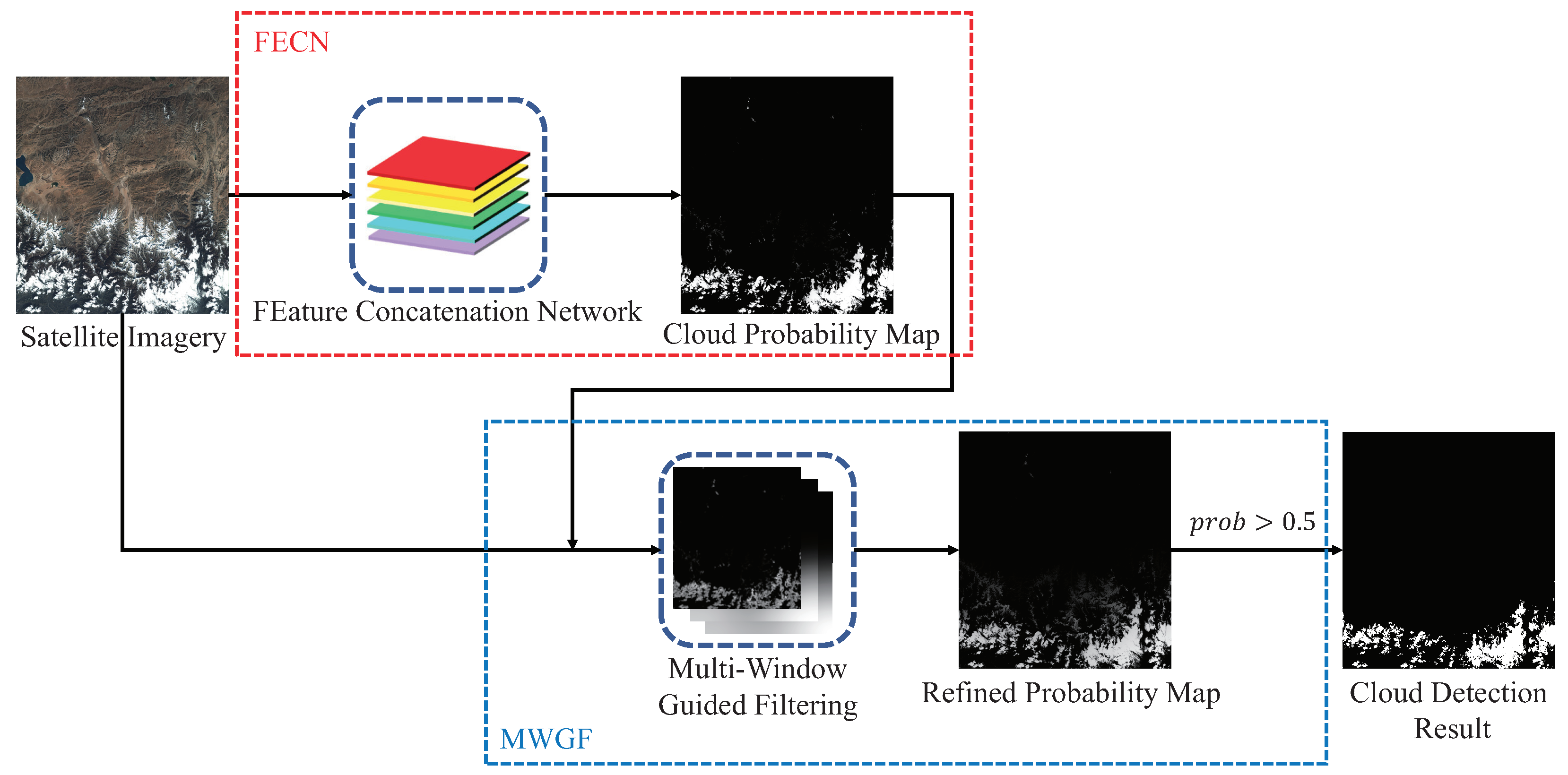
Based on these motivations, we propose our cloud detection method with two major processes (see Figure 1): the first is FEature Concatenation Network, FECN, a particular type of fully convolutional neural network, and the other is Multi-Window Guided Filtering, MWGF. In the first process, we construct the fully convolutional neural network framework based on VGG-16 and introduce extra convolution layers for producing an equal number of feature maps from different levels of the neural network. With these balanced feature maps, the final score layer in the network will explore each of them and finally give the probability map of the cloud to realize the pixel-wise prediction. In the second process, we use a composite filtering technique for better cloud refining. Guided filtering [45,46] is proved to be edge-preserved and the filtering output can learn the structure information of the guided image to some extent. Different from the previous cloud detection algorithms in [10,19], we applied filtering on cloud probability maps instead of binary cloud masks. Besides, we use multiple guided filters with different window sizes to excavate multilevel of cloud structure features and the surroundings of the imagery and to obtain better cloud masks.

The main contributions are summarized as follows,

• FEature Concatenation Network for cloud detection. Since different levels of the network contain different levels of image information, the final cloud detection results can be improved by making decisions from the concatenated features for the full use of the image information. Extensive experiments are conducted to compare different forms of utilizing multilevel features and the specific types of the network.
• Multi-Window Guided Filtering for better cloud mask refining. Different from the conventional guided filtering, the proposed filtering technology excavates multilevel structural features from the imagery. Filters with smaller window sizes can capture smaller structure features, especially the details of the imagery, while the filters with larger window sizes can grasp larger structure information, which seems to be the first-glance cloud distribution of the whole imagery. By combining the refined cloud probability maps filtered by different window sizes, the final cloud masks can be improved.
• A novel cloud detection method on satellite images for Big Data Era. The proposed cloud detection method utilizes multilevel image features by combining FEature Concatenation Network and Multi-Window Guided Filtering. Our method can outperform other state-of-the-art cloud detection methods qualitatively and quantitatively on a challenging dataset with 502 GF-1 WFV images, which contains different land features such as ice, snow, desert, sea and vegetation and is the largest cloud dataset to the best of our knowledge.

The following content is structured as follows. An introduction to the framework of fully convolutional network is given in Section 2. In Section 3 and Section 4, FECN and MWGF are introduced respectively. In Section 5, experiments about the proposed cloud detection method are conducted with discussion and analysis. Finally, Section 6 concludes this paper.

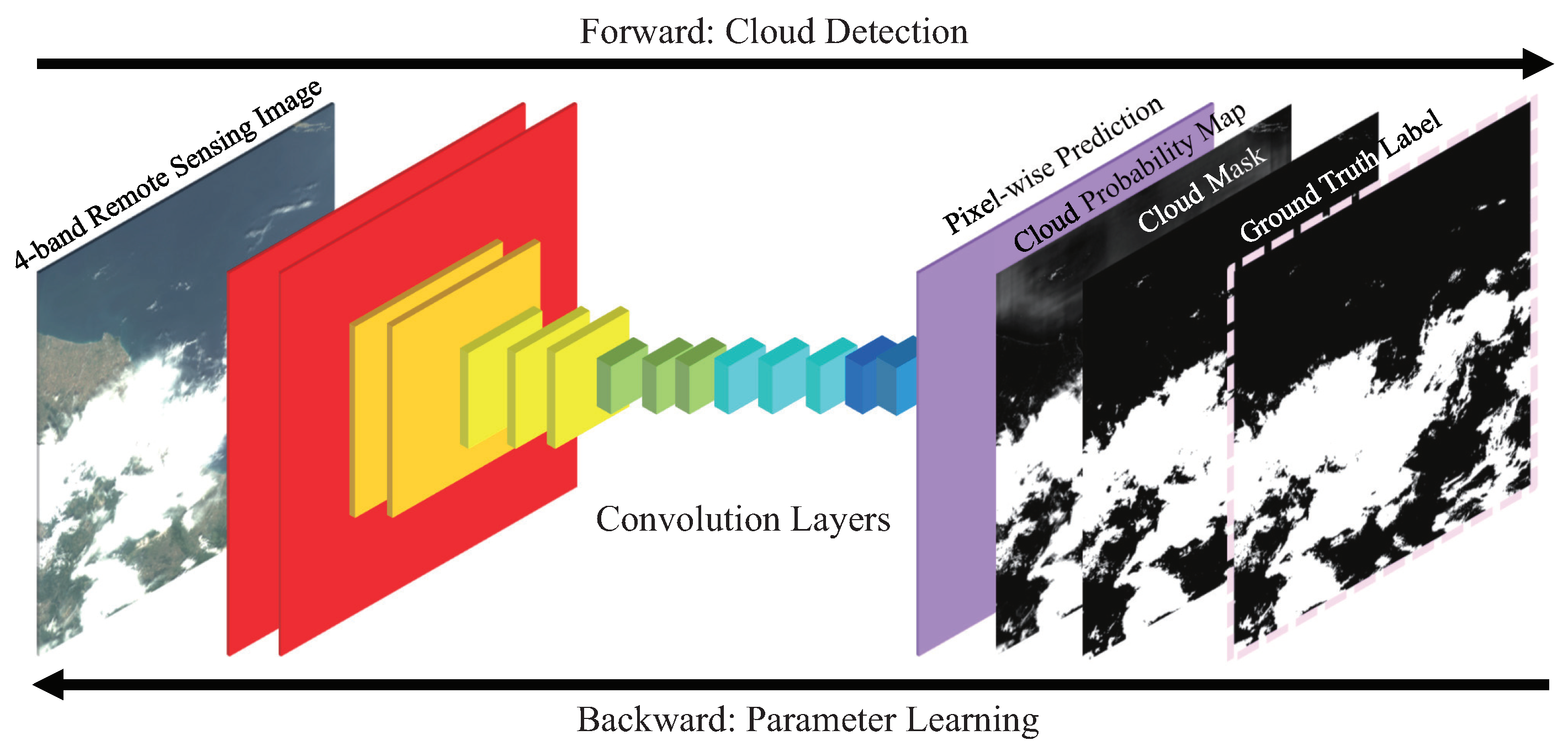
2. The Framework of Fully Convolutional Networks

DCNN is effective in a majority of patch-based image processing applications, such as image classification and object detection. The definition of patch-based image processing application is that we need to design methods for recognizing the whole or part of the image into a category. For image segmentation, which is a pixel-based image processing application, DCNN is often required to recognize every pixel of one image, therefore Fully Convolutional Networks (FCN) [41] is created. Different from DCNN, FCN predicts a label map with the same size as the input image. Figure 2 shows a typical FCN framework for cloud detection.

Similar to traditional convolutional neural networks, there are network layers in the structure of fully convolutional networks. Typically, convolution layers, pooling layers and activation layers are the main part of the network layers. Besides, softmax layers are on the bottom of the network structure for producing output label maps and cross entropy loss layers are used for training. Inputs of the network are vectors $I=[I^1;I^2;\dots ;I^b]$, where every $I^i$ ($i=1,2,\cdots ,b$) is a BGRI (blue, green, red and infrared) image cube with size $4\times h\times w$ and b is the number of image batches.

There are many convolution layers processing input data I inside the fully convolutional network structure. Convolution layers are combined with convolutional kernel matrices K. Through the lth convolution layer, input data $M^l$ of this layer will be affected by the convolutional kernel matrices $K^l$ with the following calculation,

$$M^{l+1}=M^l\ast K^l,$$

(1)

where * is a multi-dimensional convolution operator and the output is $M^{l+1}$. Based on covolution layers, high-level features maps which are the output matrix $M^{l+1}$ in the above Equation  (1) can be extracted.

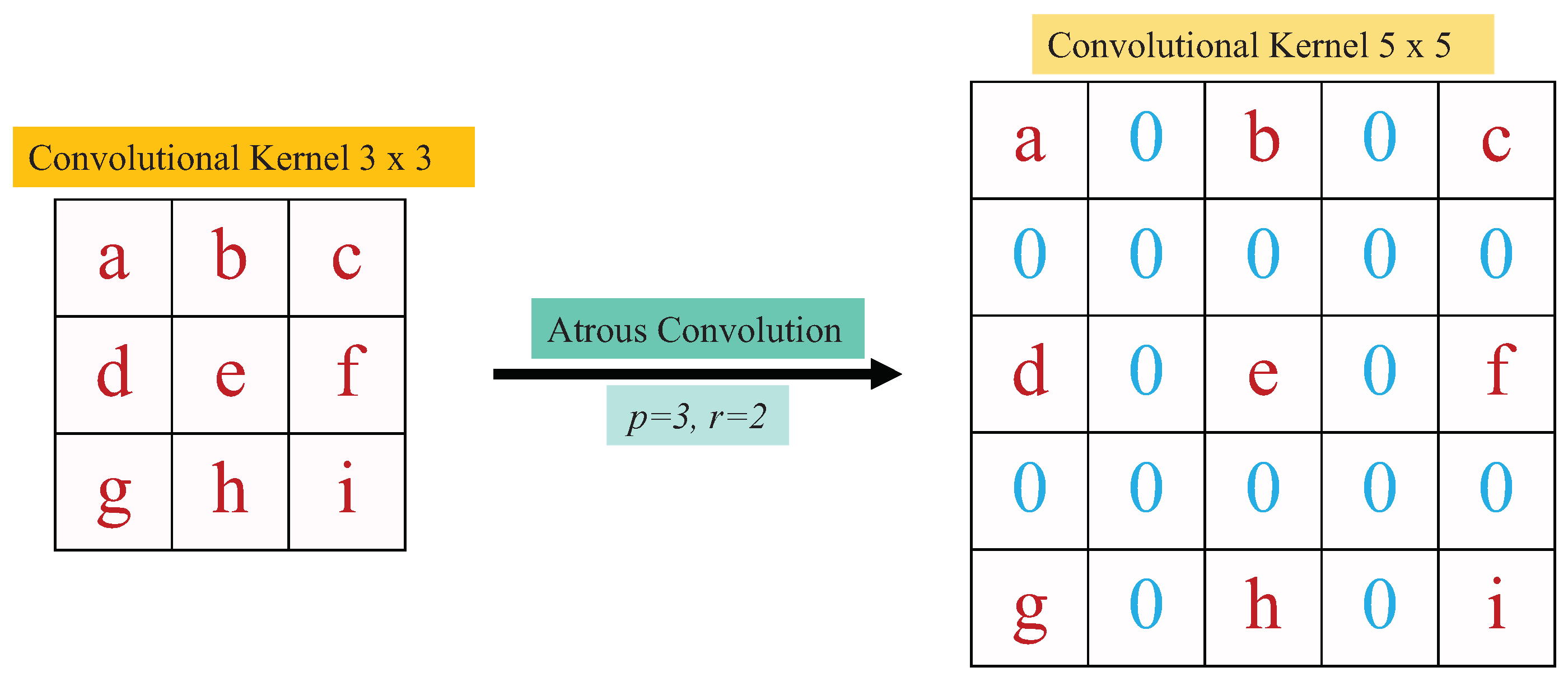
Atrous convolution [42] is also very useful in cloud detection, for it can widen the field-of-view of convolutional kernels without increasing the number of parameters for computation [4,42]. For atrous convolution, the original convolutional kernel size $p\times p$ is shifted to $[p+(p$-$1)(\mathrm{r}-1)]\times [p+(\mathrm{p}-1)(\mathrm{r}-1)]$, where r represents $r-1$ zeros introducing to the convolutional kernel between consecutive kernel values as Figure 3 illustrates atrous convolution.

Pooling layer, acting as a down-sampling filter, often follow a series of convolutional layers. It is not only designed for reducing the size of feature maps to reduce the amount of computation, but also for reducing the risk of overfitting [47]. Max pooling, which may be the most common form of pooling, is defined as the following Equation (2),

$$N_i^l=max(M_k^l),\forall k\in windo{w}_{s\times s}(i),$$

(2)

where the digital number of pixel i which belongs to the output down-sampled feature map $N^l$ is calculated by the maximum of the pixel values of $M^l$ in window (i), which size is $s\times s$. To our knowledge, the window size s is often set to 2, and several max pooling layers are installed in the framework separately.

As Equation (1) shows, convolutional layers are linear layers. Although max pooling will make the network a little nonlinear according to Equation (2), the framework still needs to be more nonlinear to fix the cloud detection tasks well. To make the learned features more expressive, as Equation (3) displays, element-wise activate functions are often settled after convolutional layers.

$$N^l=f(M^l),$$

(3)

where $M^l$ is the input features, $N^l$ is the output and $f(.)$ is the activate function. There are many types of activation functions, such as ReLU [48], ELU [49] and PReLU [50]. For computational simplicity, we use ReLU in our framework, as Equation (4) shows.

$$f(x)=max(0,x).$$

(4)

After layers of the network, deep feature maps are acquired, and classification needs to be done. In a fully convolutional network, fully connected layers in classification networks are transformed into convolution layers with $1\times 1$ kernels. Through this transformation, spatial information of the original input image is kept through the whole network. Similarly to classification neural networks, the $1\times 1$ convolutional layers produce maps of scores of each class as fully connected layers do. In our work, we distinguish these layers as “score layers”.

To value the distance of the network output and the label, softmax layer is used to produce the probabilities, as Equation (5) shows,

$$P^c=\frac{e^{S^c}}{{\sum }_{i=1}^C{e}^{S^i}},$$

(5)

where C is the number of categories, and S and P are input and output of the softmax layer respectively. In detail, $S^c$ is the score map of class c produced by score layers and $P^c$ represents the probability map of the corresponding class. In cloud detection tasks, C is set to 2, as the pixel is either cloud pixel or non-cloud pixel. Therefore, if the probability of cloud of one pixel in the input image is more than $0.5$, this pixel is classified into cloud pixel.

Loss layers are installed in the network for the purpose of making the network trainable. As many image segmentation tasks do, cross entropy loss layer is employed in our work to connect the predicted maps and ground truths. Equation (6) shows the loss function, where $y^c$ denotes the ground truths. Here, the target of training the network is to minimize this loss L. Gradients are calculated and back-propagation technologies are used for gradient delivering and convolutional kernel updating. The process is conducted iteratively and the network will run in the training phase.

$$L=-\sum _{i=1}^C{y}^{c}log(P^c)$$

(6)

Table 1. Baseline Network Configuration.

Layer Group	Layer Name	Remarks
	conv1_1, conv1_2	kernel size: $3\times 3$, kernel nums: 64
conv_block 1	pool1	pooling size: $3\times 3$, stride: 2
	conv2_1, conv2_2	kernel size: $3\times 3$, kernel nums: 128
conv_block 2	pool2	pooling size: $3\times 3$, stride: 2
	conv3_1, conv3_2, conv3_3	kernel size: $3\times 3$, kernel nums: 256
conv_block 3	pool3	pooling size: $3\times 3$, stride: 2
conv_block 4	conv4_1, conv4_2, conv4_3	kernel size: $3\times 3$, kernel nums: 512
conv_block 5	conv5_1, conv5_2, conv5_3	kernel size: $3\times 3$, kernel nums: 512, atrous: 2
	conv6	kernel size: $4\times 4$, kernel nums: 512, atrous: 4
conv_block 7	conv7	kernel size: $3\times 3$, kernel nums: 4096
score_block	score_layer	kernel size: $1\times 1$, kernel nums: 2

lists the baseline of the network almost as [44] did. In Table 1, ReLU layers are used right after each convolution layer but not listed for simplicity.

3. FEature Concatenation Network for Cloud Detection

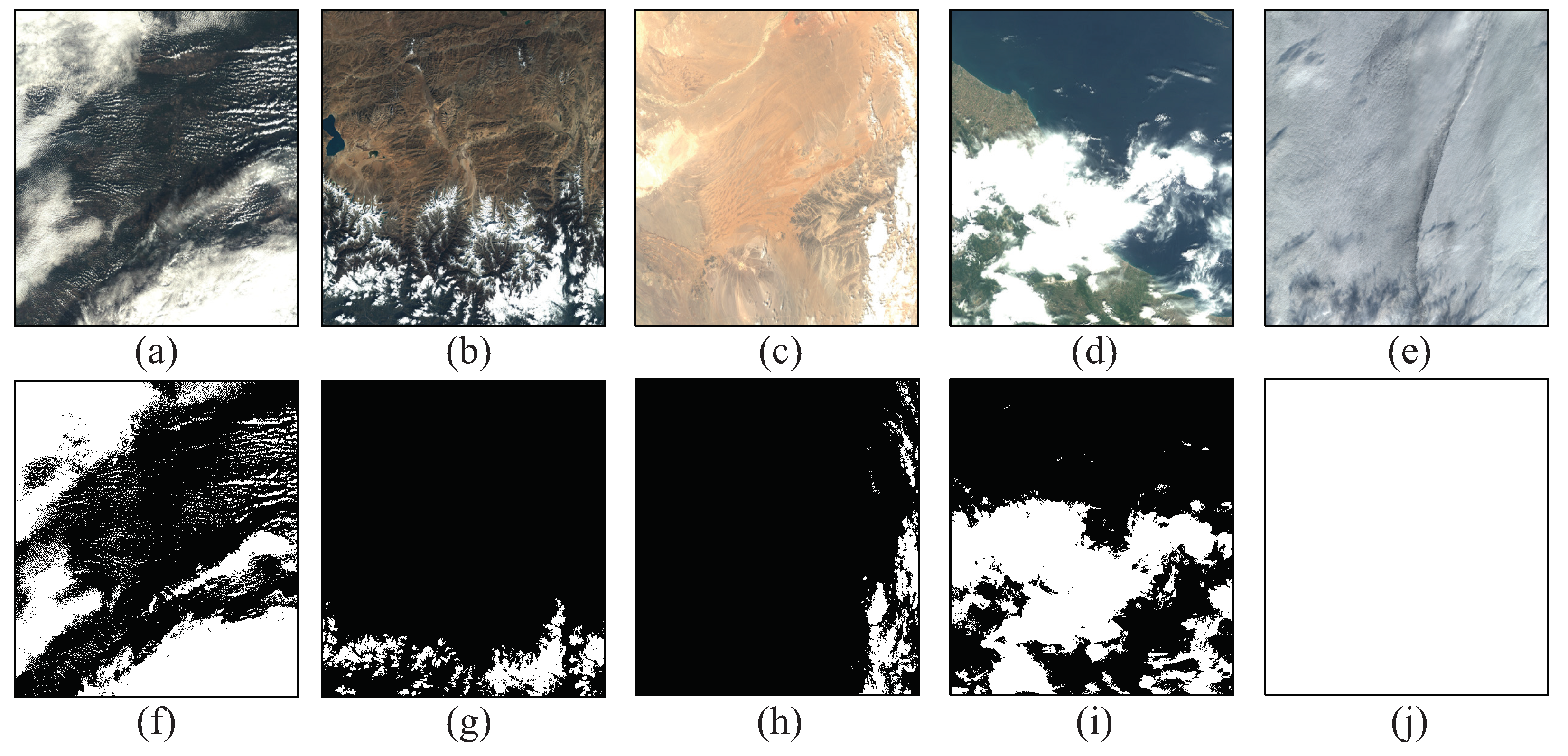
Cloud detection is not an easy task, for not only should the algorithm detect whether there are clouds in the image, but also where the clouds are in the images. FCN in the previous section is a relatively good algorithm for cloud detection, as it can extract multilevel features of the images and obtain cloud masks. In the early stages of the network, as the downsampling rate is low and the image has not passed enough convolutional layers, the information of boundary and texture of the satellite images is clear, while in the late stages, the effectiveness of deep convolutional layers and pooling layers assists the network in learning the background information and leads to more abstract features, which are close to the final classification information. However, in the satellite imagery, there are a variety of clouds from tiny ones to enormous ones above different types of land covers such as common land, snow, desert, sea and even clouds, as Figure 4 shows. The baseline FCN only analyzes the features in the late stages, which contain blurred boundary and texture of the image, according to Table 1. Therefore, the baseline FCN should be optimized to be moderate for cloud detection tasks.

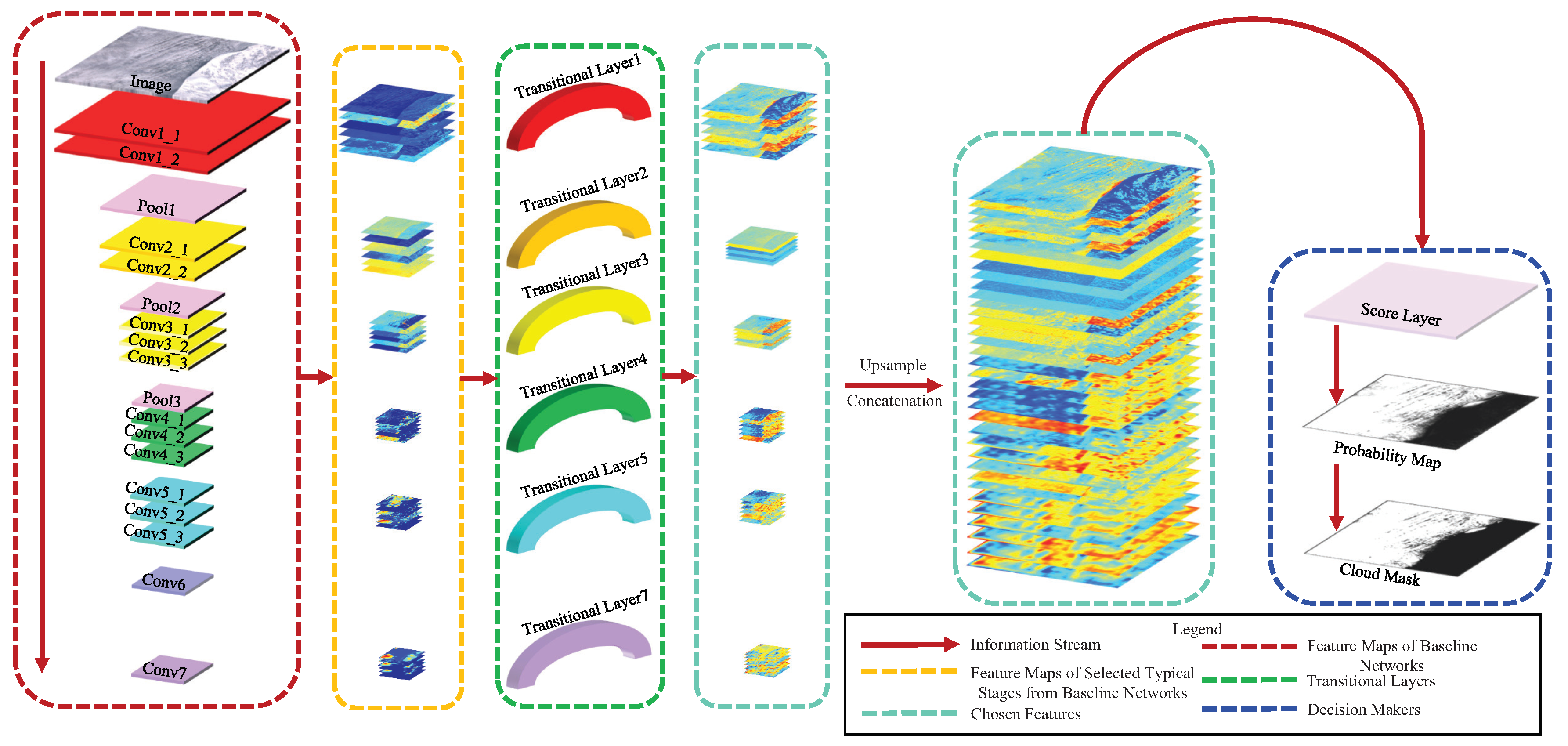
In our work, we collect multilevel features from the baseline network and make the score layer decide which features are essential for cloud detection. As Figure 5 illustrates, we add Transitional Layers right after several typical convolution layers of the baseline network for a dimensional transformation. These convolution features extracted by the added convolutional Transitional Layers are viewed as Chosen Features from the baseline network. We concatenate Chosen Features into one synthetical feature vector, where it contains both simple boundary, texture features together with deep, abstract features. Therefore, the score layer should carefully choose the decisive features in the synthetical feature vector instead of only choosing the features in the late stages of the baseline network. It is also worth noting that because the number of feature maps in the baseline network is different, we design Transitional Layers to balance the feature dimensions of all the different feature maps. For most convolutional networks, the number of low-level features is often less than that of high-level features. For instance, there are 64 feature maps produced by the low-level ‘conv1_2’ but 4096 feature maps produced by the high-level ‘conv7’ (see Table 1). Considering that features in every level should be in the same significance in the cloud detection tasks, we make a dimensional transformation by adding convolutional Transition Layers, and therefore the numbers of feature maps produced by the extra convolution layers are the same. As we concatenate multilevel features in the baseline network, we call our optimized network FEature Concatenation Network, FECN.

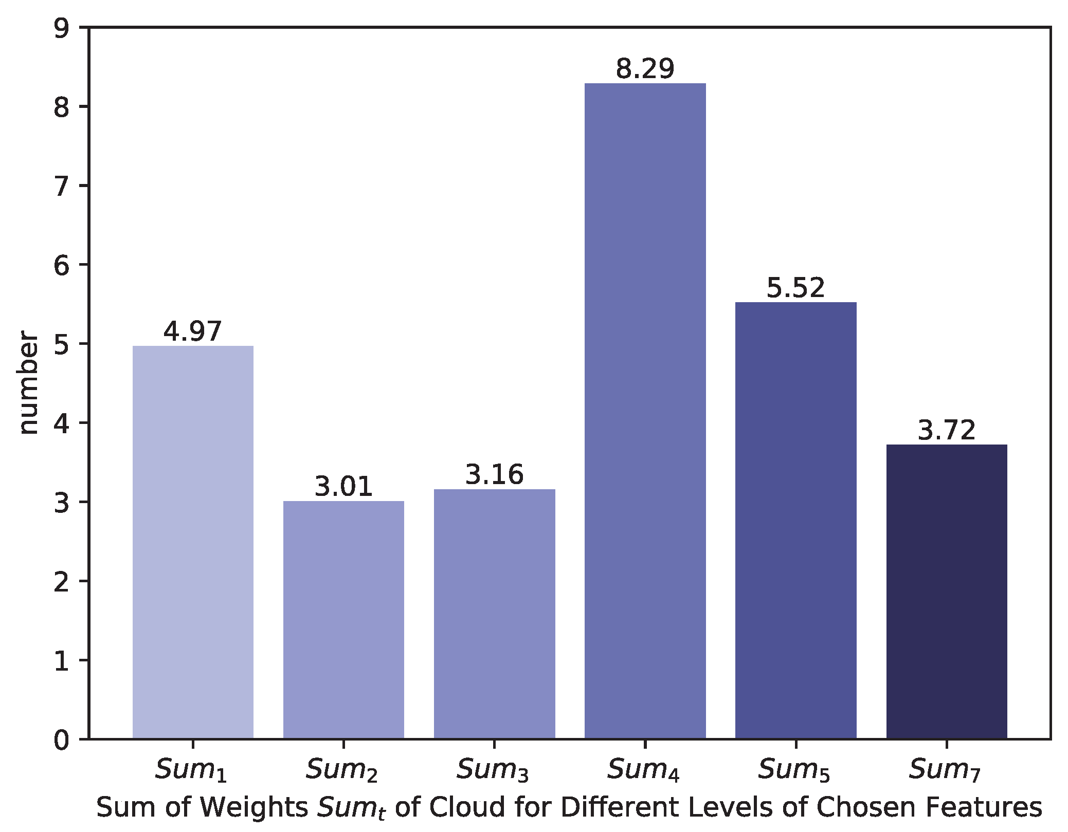
In detail, we add Transitional Layers with $3\times 3$ kernels after convolutional layers ‘conv1_2’, ‘conv2_2’, ‘conv3_3’, ‘conv4_3’, ‘conv5_3’ and ‘conv7’ in FECN, and set the score layers after Chosen Features are concatenated, as Figure 5 displays. For the limitation of GPU memory, the number of Chosen Features after each Transitional Layer is set to 64. Before Chosen Features are concatenated, they are upsampled to the original image size bilinearly.

4. Multi-Window Guided Filtering for Cloud Detection

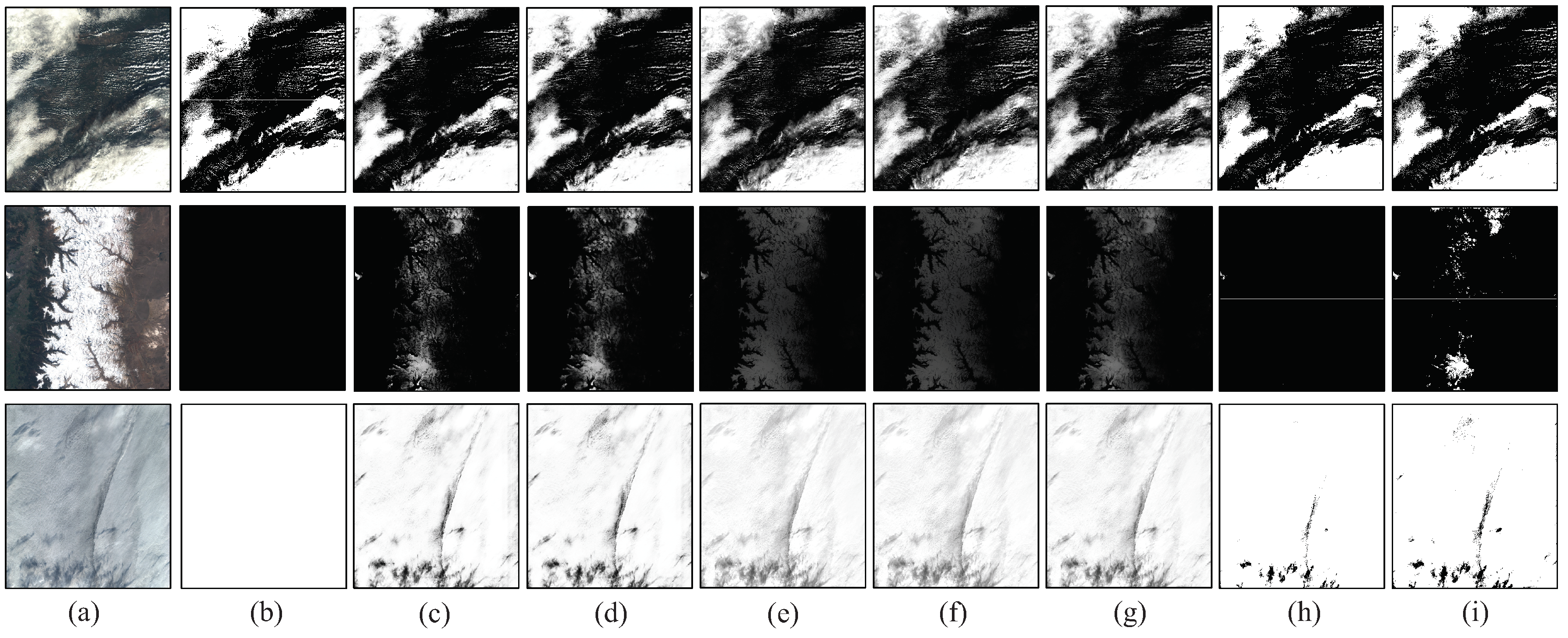
Although FECN works quite well for cloud detecting in most cases, there is still space for improvement. In most cases, FECN can obtain fine cloud masks for it analyzes multilevel features. However, for some difficult cases, such as a wide range of snow or cloud shadows due to multiple layers of clouds, FECN may get unsatisfying results as Figure 6 shows. Guided filtering [45,46], which is in $O(n)$ time complexity, can excavate the potential of the guided image and may refine the input image. It is also applied in remote sensing image processing [10,19]. Considering the characteristics of guided filtering, we concentrate on it and extend it into a composite filtering technique, Multi-Window Guided Filtering (MWGF), which involves cloud structure features and the surroundings in multilevel filtering window sizes. It can improve the results acquired by FECN in cloud detection tasks.

MWGF for cloud detection is an extended version of guided filtering [45,46], which combines multiple guided filters to excavate multilevel image features. Guided filtering involves a guidance image and another input image which needs to be filtered, and it outputs the refined image. In our work, the probability map P acquired by FECN is decisive and significant. Therefore, we set it as the input image to be filtered. To utilize all the information of the original image, we create Y the guidance image, which is defined as follows:

$$Y=\frac{B+G+R+NI}{4}$$

(7)

where B, G, R, $NI$ are the blue band, green band, red band and near-infrared band of the remote sensing image, respectively.

In MWGF, L guided filters are used. For a single guided filter, it is a local linear model, i.e., there is a linear connection between $Q^l$ and Y, where l ranges from 1 to L. For a certain pixel k of a window $w_k^l$ in image Y:

$$Q_i^l=u_k^l{Y}_i+v_k^l,\forall i\in w_k^l,$$

(8)

where $u_k^l$ and $v_k^l$ are coefficients to be calculated from the input image P. To determine the linear coefficients $u_k^l$ and $v_k^l$, we view $Q^l$ as the input P subtracting some additive noise H:

$$Q_i^l=P_i-H_i.$$

(9)

Then we minimize the differences with Equation (8). In detail, we minimize the cost function below in the window $w_k^l$:

$$E(u_k^l,v_k^l)=\sum _{i\in w_k^l}({(u_k^l{Y}_i+v_k^l-P_i)}^2+ϵ{u_k^l}^2).$$

(10)

In this equation, $ϵ$ is a regularizer penalizing $u_k^l$. Here, a solution to Equation (10), the linear ridge regression model [51,52], is given by

$$u_k^l=\frac{\frac{1}{|w^l|}{\sum }_{i\in w_k^l}{Y}_i{P}_i-{\mu }_k^l\overline{P_k}}{{{\sigma }_k^l}^2+ϵ},$$

(11)

$$v_k^l=\overline{P_k}-u_k^l{\mu }_k^l,$$

(12)

where ${\mu }_k^l$ and ${\sigma }_k^l$ represent mean and variance value of Y in $w_k^l$, $\overline{P_k}$ is the mean value of P in $w_k^l$ and $|w^l|$ denotes the number of pixels in $w_k^l$. Considering a pixel i is computed for times in the moving overlapping windows $w_k^l$ that covers pixel i, there exists a strategy to reduce the complexity to compute $Q_i^l$ by averaging (${\mu }_k^l$,${\sigma }_k^l$) for all windows $w_k^l$ in the image. Thus, the final output $Q_i^l$ for a certain window size $w^l$ is defined as the following:

$$Q_i^l=\overline{u_k^l}{Y}_i+\overline{v_k^l},$$

(13)

where $\overline{u_k^l}=\frac{1}{|w^l|}{\sum }_{k\in w_i^l}{u}_k^l$ and $\overline{v_k^l}=\frac{1}{|w^l|}{\sum }_{k\in w_i^l}{v}_k^l$ are the average coefficients of windows which contain the pixel i.

Here, we find that $\overline{u^l}$ is a representative feature of cloud structure and the surroundings as Figure 7. This is because $\overline{u^l}$ is a transform of both Y and P. For smaller windows, P seems to play a more important role and $\overline{u^l}$ concentrates on the structure of small clouds or the edges of large clouds, mainly the details of the imagery, while for larger windows, more information of Y involves and $\overline{u_k^l}$ denotes the structure of larger clouds and even part of the background, which seems to be the first-glance cloud distribution of the imagery. Therefore, the final refined probability map $Q^l$ is also different. For smaller windows, the output is closed to the input P, which keeps the original clouds as Figure 8c illustrates, while for the larger windows, the output excavates more about the guided image Y, which smooths the input P to some extent as Figure 8d,e show.

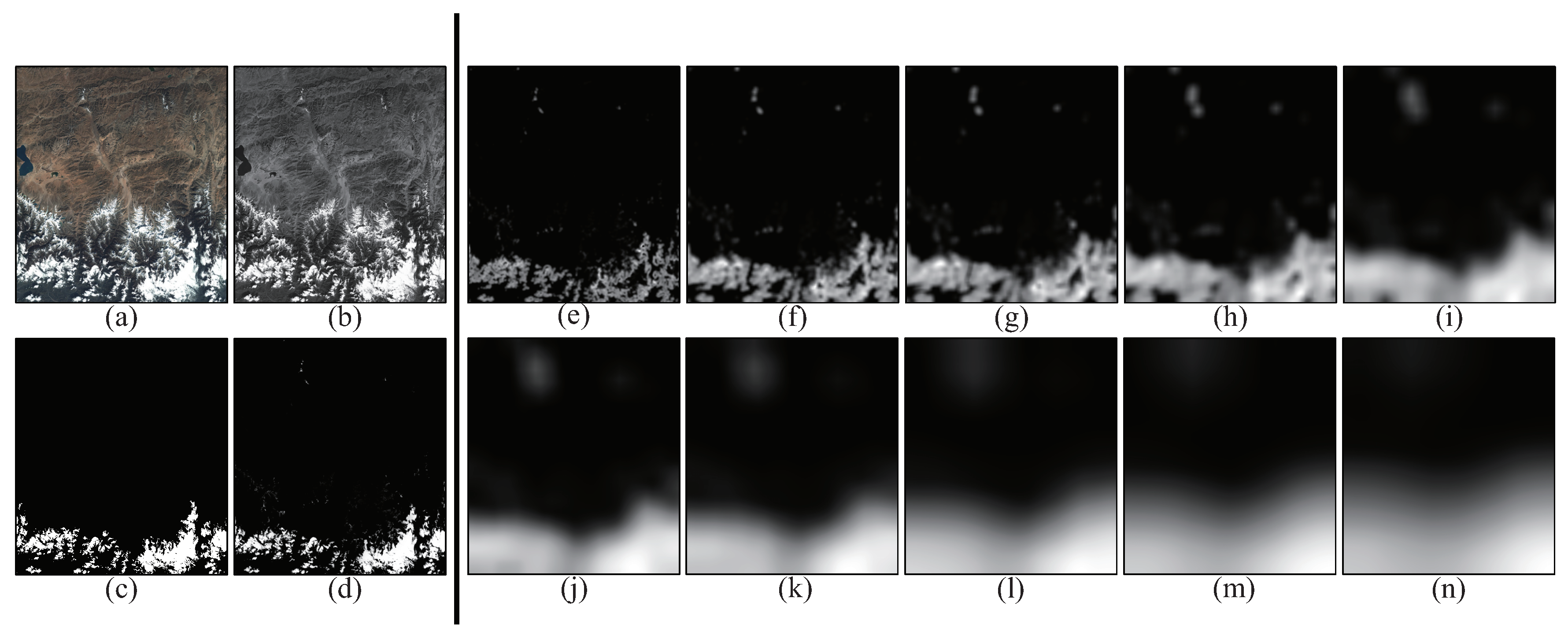
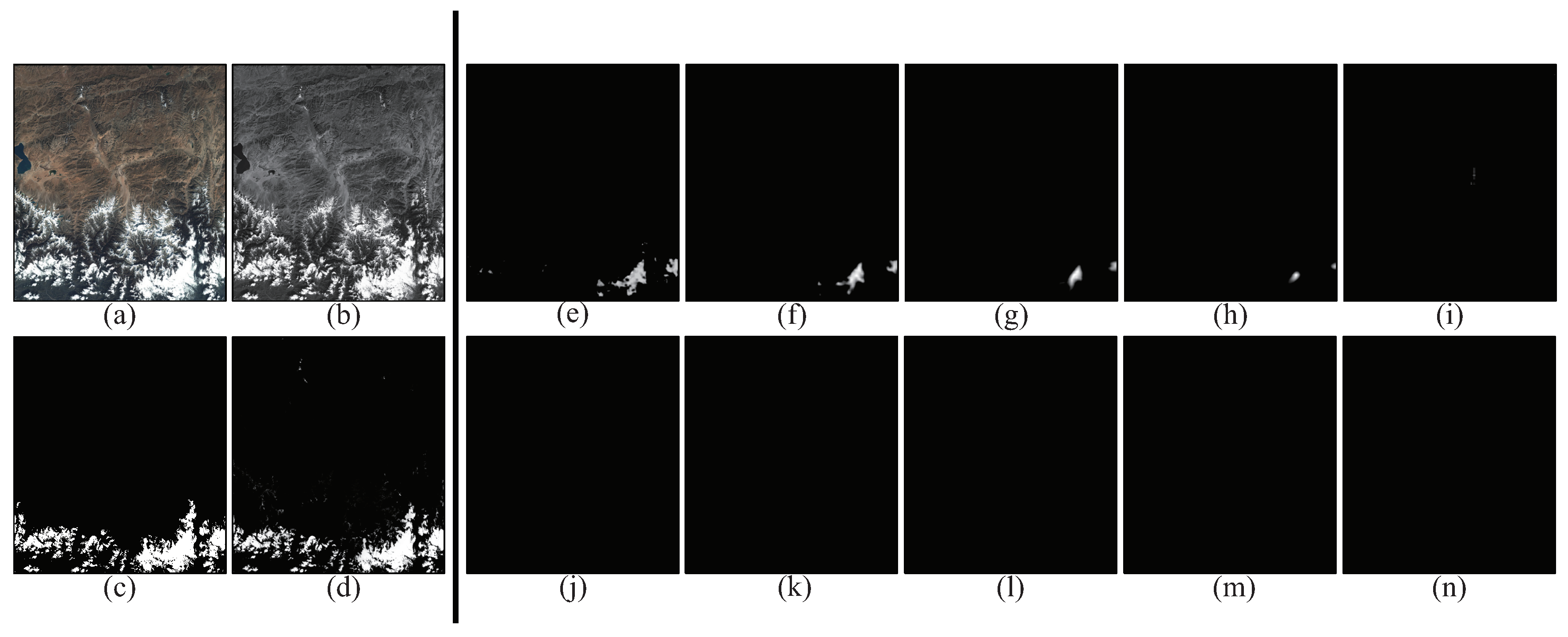
We also find that $\overline{v^l}$ is a supplementary representative feature of $\overline{u^l}$. For larger windows as Figure 9j–n show, $\overline{v^l}$ almost equals nothing. This is because the guided image Y changes a lot within the larger windows $w_k^l$, and ${{\sigma }_k^l}^2\gg ϵ$. Thus, we have

$$\begin{array}{cc}\hfill u_k^l{\mu }_k^l=& \frac{\frac{1}{|w^l|}{\sum }_{i\in w_k^l}{Y}_i{P}_i-{\mu }_k^l\overline{P_k}}{{{\sigma }_k^l}^2+ϵ}{\mu }_k^l\hfill \\ \hfill \approx & \frac{\frac{1}{|w^l|}{\sum }_{i\in w_k^l}{Y}_i{P}_i-{\mu }_k^l\overline{P_k}}{{{\sigma }_k^l}^2}{\mu }_k^l\hfill \\ \hfill =& \frac{\frac{1}{|w^l|}{\sum }_{i\in w_k^l}{Y}_i{P}_i(\frac{1}{|w^l|}{\sum }_{i\in w_k^l}{Y}_i)-{{\mu }_k^l}^2\overline{P_k}}{{{\sigma }_k^l}^2}\hfill \\ \hfill =& \frac{\frac{1}{|w^l|}{({\sum }_{i\in w_k^l}{Y}_i)}^2-{{\mu }_k^l}^2}{{{\sigma }_k^l}^2}\overline{P_k}\hfill \\ \hfill =& \overline{P_k}.\hfill \end{array}$$

(14)

According to the above Equations (12) and (14), we can easily draw the conclusion that $\overline{v^l}\approx 0$ in larger windows. Therefore, in the method of MWGF for cloud detection tasks, $\overline{u^l}$, a representative feature of cloud structure and the surroundings, plays the most significant role in calculating $Q^l$.

After calculating $Q^l$ of all the windows, we should summarize them to form a final refined probability map Q. In our work, we average every $Q^l$ to acquire Q as the following Equation (15).

$$Q=\frac{1}{L}\sum _{l=1}^L{Q}^l$$

(15)

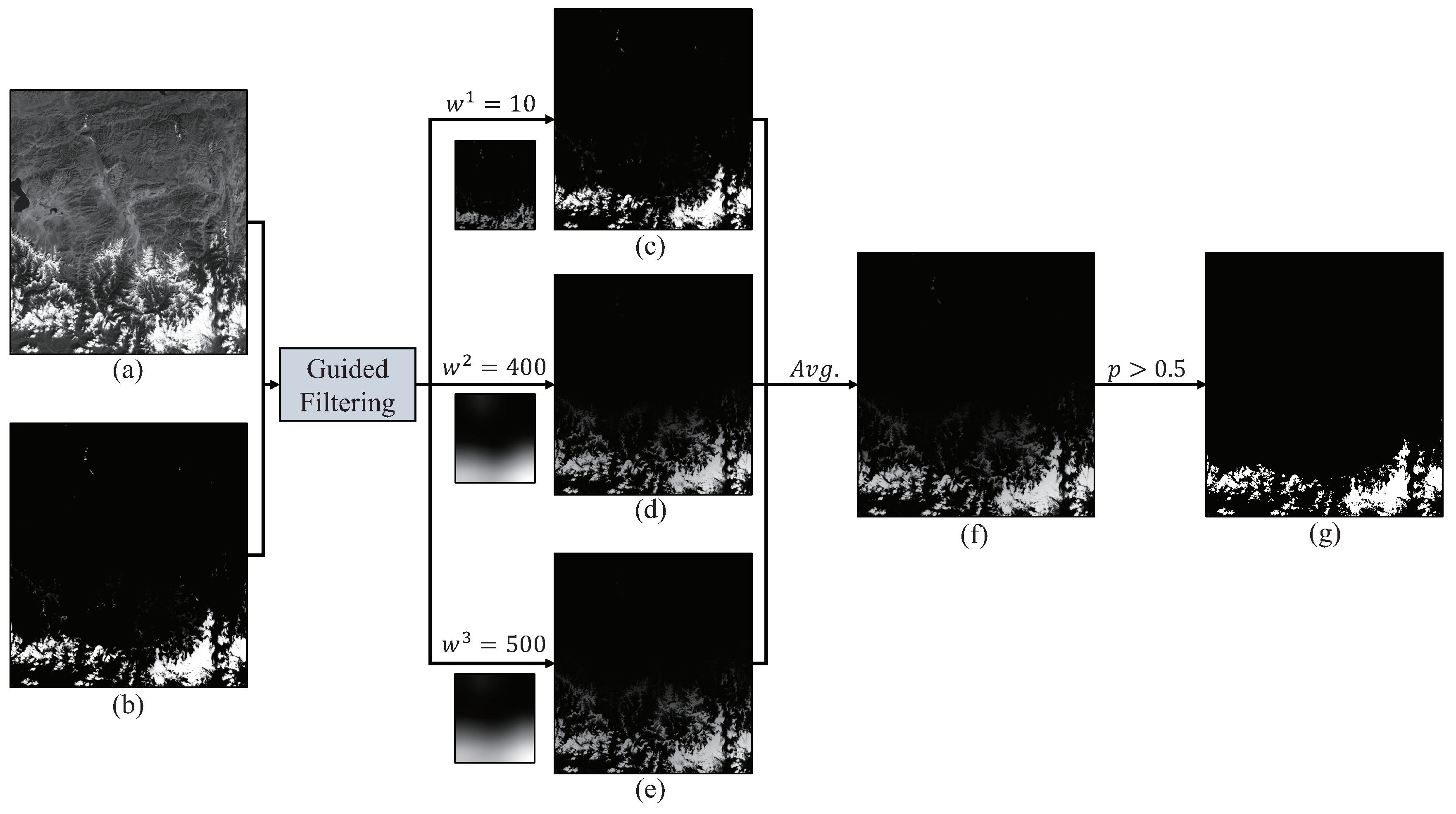
To make our method effective, we examine different window size combination and finally choose them to be the combination of 10, 400 and 500. We also set $ϵ$ = 1 ×${10}^{-6}$. The following Algorithm 1 is the algorithm of MWGF and Figure 8 displays its process.

Algorithm 1 Multi-Window Guided Filtering for Cloud Detection Result Refining

Input: Cloud probability map P acquired by FECN, the original remote sensing image I, filtering window sizes $w^1$, $w^2$, ..., $w^L$, and penalizing regularizer $ϵ={10}^{-6}$. Procedures: 1. Calculate Y with I according to Equation (7). 2. Calculate $Q^l$ with Y for each window size ranging from $w^1$ to $w^L$ based on Equations (11)–(13). 3. Average $Q^1,Q^2,\cdots ,Q^L$ and form the final refined cloud probability map Q based on Equation (15). Output: the final refined cloud probability Q.

5. Experiments and Discussion

5.1. Dataset

To evaluate the effectiveness of our cloud detection method quantitatively, 502 GF-1 WFV remote sensing images downloaded from http: //www.cresda.com/ are collected to build the dataset. To the best of our knowledge, it is the largest cloud dataset so far. For one GF-1 WFV image, it has 4 bands as

Table 2. GF-1 WFV parameters.

Items	Parameters
Band 1 (blue)	0.45∼0.52$\mathsf{\mu }$m
Band 2 (green)	0.52∼0.59$\mathsf{\mu }$m
Band 3 (red)	0.63∼0.69$\mathsf{\mu }$m
Band 4 (infared)	0.77∼0.89$\mathsf{\mu }$m
Ground Sample Distance	16 m
Swath Width	830 km

shows and its size is $13,400\times 12,000$ pixels. These images, which were acquired from May 2013 to December 2016, were chosen in different global regions as Figure 10 shows and they contain different land features such as ice, snow, desert, sea and vegetation. In our experiment, the training set contains 402 images and the 100 images are in the testing set. To the best of our knowledge, it is the largest cloud dataset with manually labeled ground truths. The ground truths in the whole dataset are obtained manually. We first transfer the original image into RGB 24-bit color image, then use the Adobe Photoshop software as [19] did to label them into two categories, cloud and background. Figure 10 is an illustration for the distributions of training and testing data.

5.2. Experiment Setup and Benchmark Metrics Setup

In this paper, all the deep learning networks are implemented with PyTorch0.31 [53] on Ubuntu 16.04 with an NVIDIA Geforce GTX 1080 Ti GPU card. The networks are trained in stochastic gradient descent method with initial learning rate as 0.005. The learning rate decay policy is set to “poly”, and the power parameter is set to 0.9. We set the training batch size as 4 and the training iteration number as ${10}^6$. Convolution weights of the networks are initialized by “msra” method [50]. In the training procedure, we also use random rotation ($0^{\circ }$, $90{}^{\circ }$, ${180}^{\circ }$, ${270}^{\circ }$) as a data augmentation technique.

To evaluate the performance of different methods, we adopt those five benchmark metrics Accuracy (A), Probability of Detection (POD), False Alarm Ratio (FAR), Hansen Kuipers Discriminant (HK) and Intersection-Over-Unions (IOU) which are widely used in cloud detection tasks. These metrics are defined as Equations (16)–(20) respectively, where TCP is the abbreviation for True Cloud Pixels recording the number of pixels which are the correct cloud pixels, FCP is the abbreviation of False Cloud Pixels recording the number of pixels which are recognized incorrectly as cloud (in fact, these pixels should be recognized as background), and FBP is False Background Pixels recording the number of pixels which are recognized incorrectly as background (in fact, these pixels should be recognized as cloud).

$$A=\frac{TCP}{TCP+FCP}$$

(16)

$$POD=\frac{TCP}{TCP+FBP}$$

(17)

$$FAR=\frac{FBP+FCP}{TCP+TBP+FBP+FCP}$$

(18)

$$HK=\frac{(TCP\ast TBP)-(FCP\ast FBP)}{(TCP+FCP)\ast (TBP+FBP)}$$

(19)

$$IOU=\frac{TCP}{TCP+FBP+FCP}$$

(20)

5.3. Effectiveness of FEature Concatenation Network

5.3.1. Comparisons between Two Ways of Utilizing Multilevel Feature Information

There are two main ways to utilize multilevel features obtained from the convolutional neural networks. As Figure 11 shows, one is utilizing multilevel probability maps (Figure 11a) and the other is concatenating multilevel feature maps (Figure 11b). In detail, after the original image passes through the baseline convolutional network, the method of Figure 11a makes predictions on each of the selected convolution blocks, and then adds them all as the final prediction, while the method of Figure 11b concatenates the chosen features and makes the final prediction based on the feature vector. Therefore, we can call the two methods Prediction Fusion and Feature Concatenation, respectively. Although both ways utilize multilevel features, they do get different cloud detection results.

Figure 12 is the visual comparisons of the two different ways of utilizing multilevel features. Figure 12a,b are the original images and the corresponding ground truths. Figure 12c,d are the results of Prediction Fusion and Feature Concatenation respectively. We can see that although both methods obtain almost the same cloud detection masks on images with ordinary land cover and multilayers of clouds, Feature Concatenation outperforms in the images with snow, sea and desert. This indicates that feature concatenation works better in utilizing multilevel feature maps.

Table 3. Quantitative results of ways of utilizing multilevel feature information on testing set.

Method	A (%)	POD (%)	FAR (%)	HK (%)	IOU (%)
Prediction Fusion	90.72	87.85	3.69	88.17	80.26
Feature Concatenation (ours)	92.92	90.08	2.93	90.83	84.29

is the quantitative evaluation result of Prediction Fusion and Feature Concatenation. Due to the better A, POD, FAR, HK and IOU, we can learn that Feature Concatenation is better than Prediction Fusion in cloud detection tasks. Therefore, our method FEature Concatenation Network (FECN) is proved to be more effective in utilizing multilevel features.

5.3.2. Analysis on Different Types of FECN

FECN concatenates feature maps in the baseline network, which is verified to be more effective than prediction fusion. However, how many levels of features in FECN should be used still needs to be tested for the cloud detection task. Therefore, we conduct experiments on different types of FECN. Firstly, we train the baseline network as Table 1 configures. Then, based on the baseline network, we gradually add Transitional Layers from the 4th, 5th and 7th convolution blocks (denoted as FECN_457) to the 1st, 2nd, 3rd, 4th, 5th and 7th convolution blocks (denoted as FECN_123457).

Figure 13 shows visual comparisons of different types of FEature Concatenation Network. Figure 13a,b are the original images and the corresponding ground truths. Figure 13c, is the result of baseline network, which indicates that without combining different levels of convolution features, the cloud detection results would be rather coarse. However, with more and more bridge layers adding into the network by observing the results from Figure 13d,g, the cloud detecting mask is becoming more and more exquisite. From the visual comparisons, FECN_123457 (Figure 13g), obtains the best cloud masks.

Table 4. Quantitative results of different types of FECN on testing set.

Method	A (%)	POD (%)	FAR (%)	HK (%)	IOU (%)
Baseline	90.74	66.14	7.09	83.96	61.95
FECN_457	88.77	80.46	5.19	84.71	73.02
FECN_3457	89.08	82.02	4.90	85.34	74.53
FECN_23457	93.10	85.34	3.48	89.49	80.26
FECN_123457	92.92	90.08	2.93	90.83	84.29

is the quantitative evaluation result of different types of FECN. Although FECN_23457 achieves the best A, we can see that our network FECN_123457 is the best type of FECN due to the best POD, FAR, HK and IOU. This indicates that all levels of chosen features need to be analyzed. Therefore, our proposed FECN_123457 is a proper deep learning network for the cloud detection task and its results will be sent later to the Multi-Window Guided Filtering procedure.

We can also learn from the histogram shown in Figure 14 that all levels of chosen features are significant. Here, we make statistics of the filter weights of different chosen features to evaluate whether they contribute to the final probability map. In detail, we check the final score layer and examine the corresponding sum of weights $Su{m}_t$ of cloud for different levels of chosen features according to the following Equation (21):

$$Su{m}_t=\sum _{w\in W_t}abs(w),t=1,2,3,4,5,7$$

(21)

where t is the count of Transitional Layer and $W_t$ represents the corresponding set of cloud filter weights. As Figure 14 shows, all the chosen features take effect in the network and it also indicates that for cloud detection tasks, we need to analyze multilevel features of the deep learning network.

5.4. Benefit of Multi-Window Guided Filtering

MWGF is a filtering technique using multiple guided filters, which excavates multilevel image features with different filtering window sizes. Here we explore the influence on the combination of window sizes of MWGF. In this section, after we obtain the results from FECN_123457, we send them to different types of MWGF. There are 10 types of guided filtering window sizes: 10, 20, 30, 50, 100, 150, 200, 300, 400 and 500. We combine 1, 2, 3 or 4 types of guided filtering window sizes to form MWGF, where window sizes are not chosen repeatedly. Therefore, we obtain $C_{10}^1+C_{10}^2+C_{10}^3+C_{10}^4=385$ types of results. It should be noted that when we choose only one guided filtering window size, MWGF is degraded to Guided Filtering (GF). Here we evaluate the performance of MWGF mainly by IOU, which is widely used in the image segmentation task.

Table 5. Quantitative comparisons of different parameter settings of MWGF on the testing set.

Method	A (%)	POD (%)	FAR (%)	HK (%)	IOU (%)	Rank in IOU
FECN without filtering	92.92	90.08	2.93	90.83	84.29	—
GF_300	95.69	88.42	2.72	93.28	85.04	143rd
GF_200	95.07	88.82	2.76	92.74	84.91	249th
GF_400	95.99	88.02	2.74	93.49	84.89	254st
MWGF_10_500	94.87	89.39	2.70	92.64	85.27	8th
MWGF_20_500	94.99	89.23	2.70	92.74	85.22	20th
MWGF_10_400	94.71	89.45	2.72	92.51	85.19	32nd
MWGF_10_400_500	95.35	89.09	2.67	93.07	85.38	1st
MWGF_10_300_500	95.21	89.17	2.68	92.95	85.34	2nd
MWGF_20_400_500	95.41	88.94	2.68	93.10	85.29	5th
MWGF_10_300_400_500	95.46	88.94	2.67	93.15	85.33	3rd
MWGF_10_200_400_500	95.32	89.03	2.68	93.03	85.30	4th
MWGF_10_150_400_500	95.23	89.09	2.69	92.95	85.28	7th

shows the top-3 results of each different numbers of guided filtering window sizes. In the first column of Table 5, “MWGF_a_b_c_d” denotes that we choose more than one type of guided filtering window sizes, a,b,c and d, and “GF_a” denotes that we only choose one type of window size, a. In the last column of Table 5, the rank in IOU of all lists (385 types of window size combinations) is recorded.

From Table 5, we find that the best parameters of window size combination are 10, 400 and 500. In this parameter setting of MWGF, the IOU of the refined cloud detection masks is up to 84.29, 1.09 better than that without the filtering procedure. Therefore, we select MWGF_10_400_500 as our MWGF parameter settings. Besides, from the last column of Table 5, we know that using more than one guided filtering results with different window sizes is very effective. GF_300, which stands out in the IOU rank with only one guided filter, is in a rather low rank in IOU (143rd), and 0.34 behind the first MWGF parameter setting, MWGF_10_400_500. It indicates that using multiple guided filters can achieve stronger improvement than using only one.

It is also worth noting that tiny window size (10 or 20) and huge window size (400 or 500) are usually bundled in the top-3 MWGF results of each different number of window sizes. From Figure 15, guided filtering with tiny window size would mainly keep the original input, especially the preservation of details (Figure 15d), and probability map after guided filtering with huge window sizes would highlight the cloud area with the most confidence (Figure 15e,f). Through the combination of multiple guided filters, with different types of clouds remaining, false alarms of high reflectance area with snow are wiped out and some missing part of the cloud is recovered for images with multilevel clouds. Therefore, the cloud mask is refined through MWGF, a filter technique involves multilevel features of the images, as the comparison of Figure 15h,j indicates.

5.5. Comparison with Other Methods

In this section, we compare our method with other popular traditional cloud detection methods [10,11,19], which are based on physical information or physical information integrated with statistical techniques. Method of [19] is a typical physical method, which uses the reflectance of all band information and the relationship of bands in GF-1 WFV imagery. The method of [10,11] utilizes physical information together with statistical techniques, such as filtering refinement techniques in [10] and the use of texture information and structure information in [11]. We also compare with two methods [12,44], which are based on deep learning. The method of [12] classifies image superpixels into thick cloud, thin cloud and background, and further we combine thick cloud and thin cloud together. The method of [44] uses a structure of FCN, and it summarizes the probability map from each level of the network. It segments the image into three classes: snow, cloud and background, and further we extract the cloud mask.

Figure 16 shows visual comparisons of different methods, where the Figure 16b are the ground truths and Figure 16c–h are the results of different methods. From the visual comparisons, we can see our method performs better than other methods, especially in the difficult cases, such as images with ice, desert, snow, sea and multilayers of clouds.

For quantitative evaluation, we evaluate A, POD, FAR, HK and IOU as the previous experiments did.

Table 6. Quantitative comparisons on other traditional methods and ours on the testing set.

Method	A (%)	POD (%)	FAR (%)	HK (%)	IOU (%)
Method of [10]	29.73	54.78	30.51	18.09	23.87
Method of [11]	24.26	86.58	49.57	18.03	23.38
Method of [19]	64.51	96.77	9.86	63.75	63.15
Method of [12]	74.04	44.04	12.47	63.13	38.15
Method of [44]	79.39	77.26	7.48	74.60	64.35
Ours	95.45	89.09	2.67	93.07	85.38

shows the results, and from it we can see that our method stands out among all the methods. Although the method of [19] obtains the highest POD, the relatively worse A drags down the HK and IOU statistics. Considering that our method reaches the best A, FAR, HK and IOU, our method outperforms other compared methods, which indicates that our method suits for cloud detection by a combination of FECN and MWGF.

6. Conclusions

In this paper, we propose a novel cloud detection method by utilizing multilevel image features with two major processes. The proposed method is inspired by the utilization of multilevel features. We first set up FEature Concatenation Network, which is a deep learning network utilizing features from low-level to high-level, to get the cloud probability map. With balanced feature maps from different levels concatenated, the final cloud probability map explores the image information from every level. Further, we refine the cloud probability map by a composite filtering technique, Multi-Window Guided Filtering, which excavates multilevel cloud structure features and the surroundings. By combining the refined cloud probability maps filtered by different window sizes, the refined cloud masks can be improved.

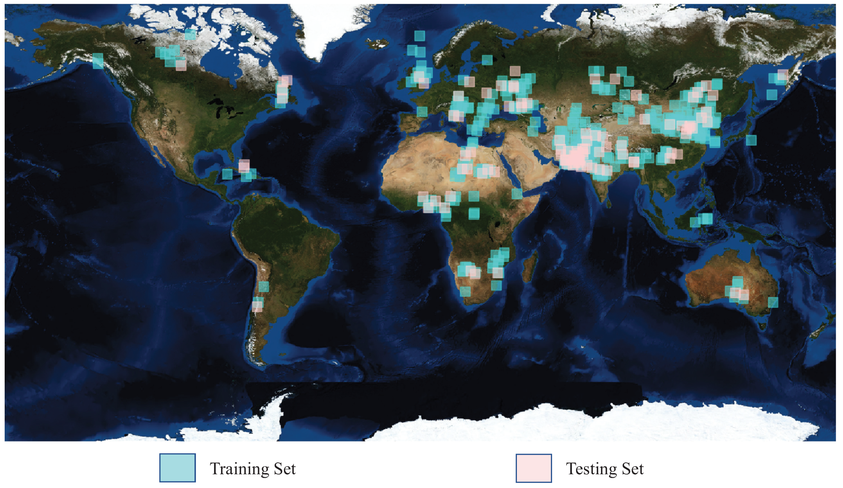
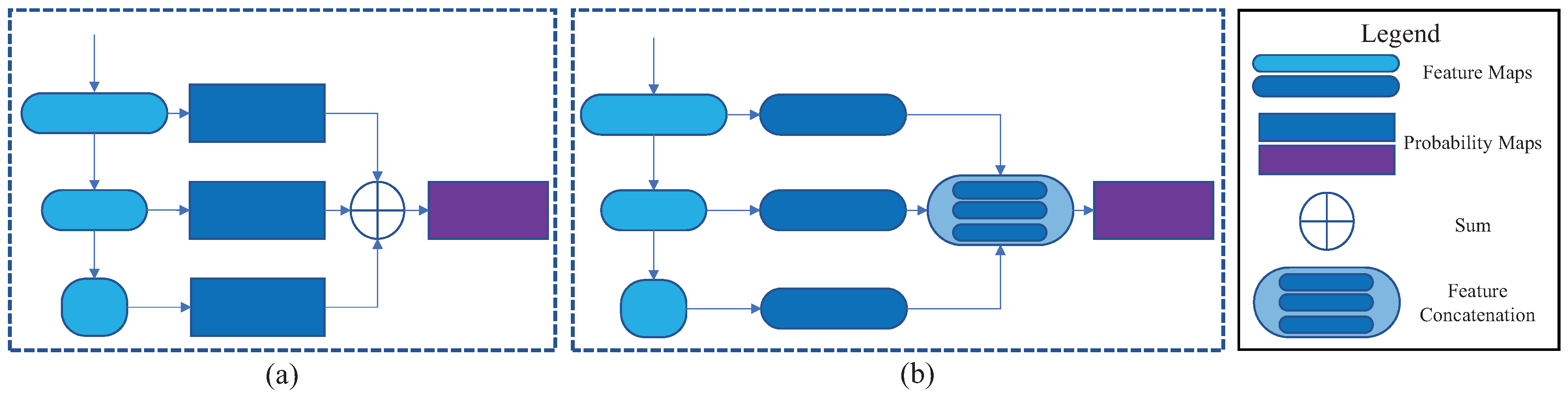
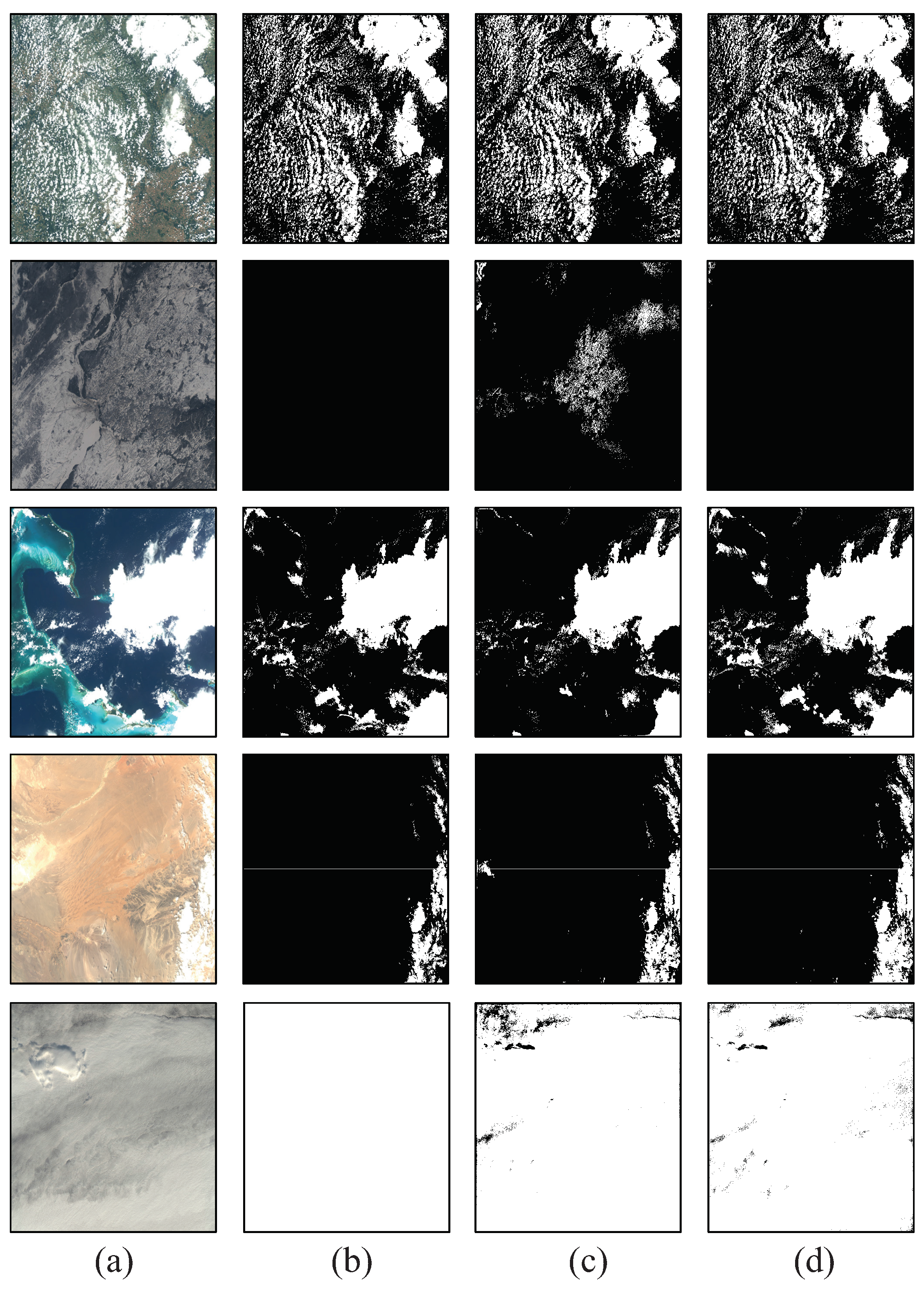
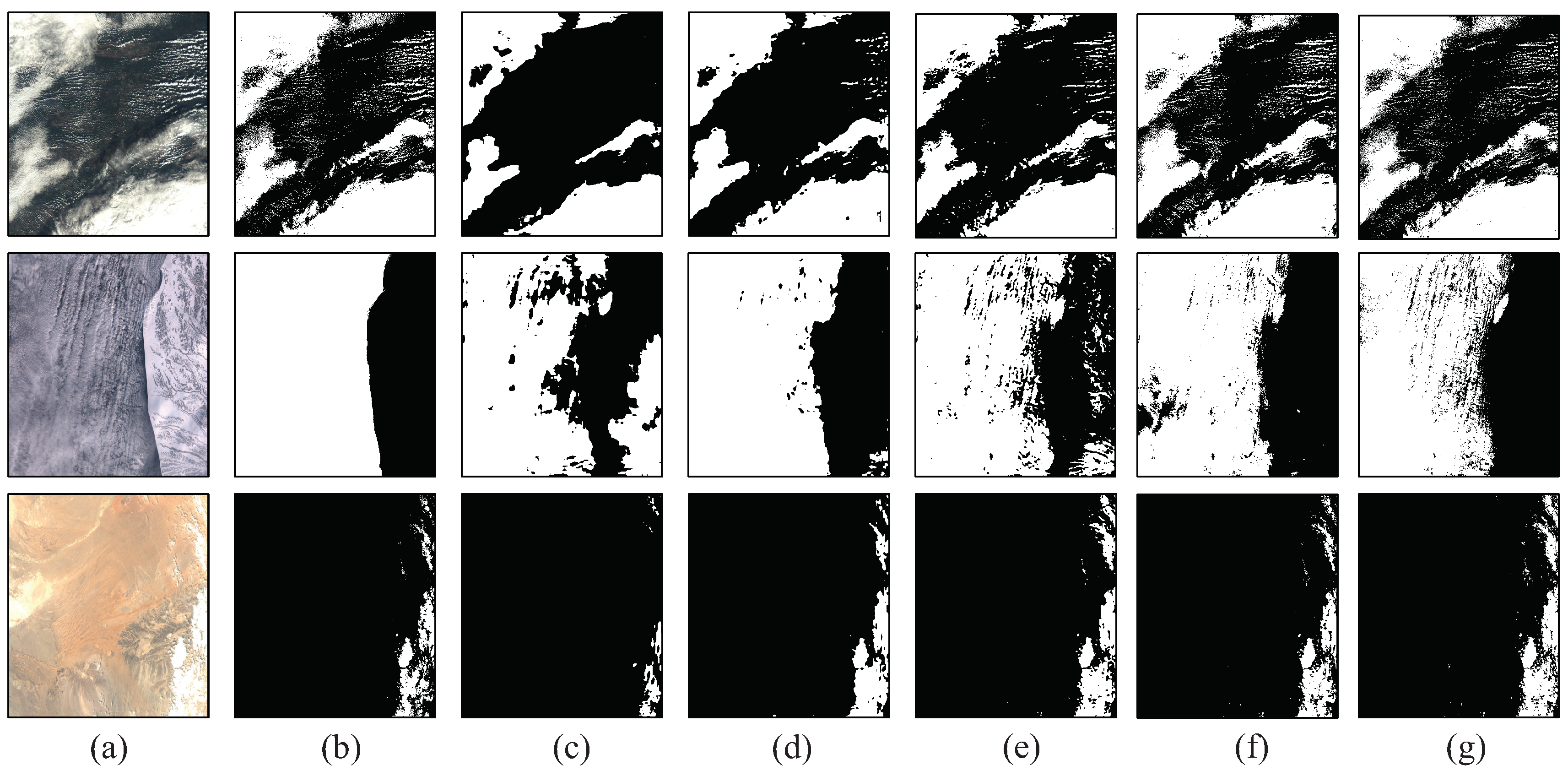
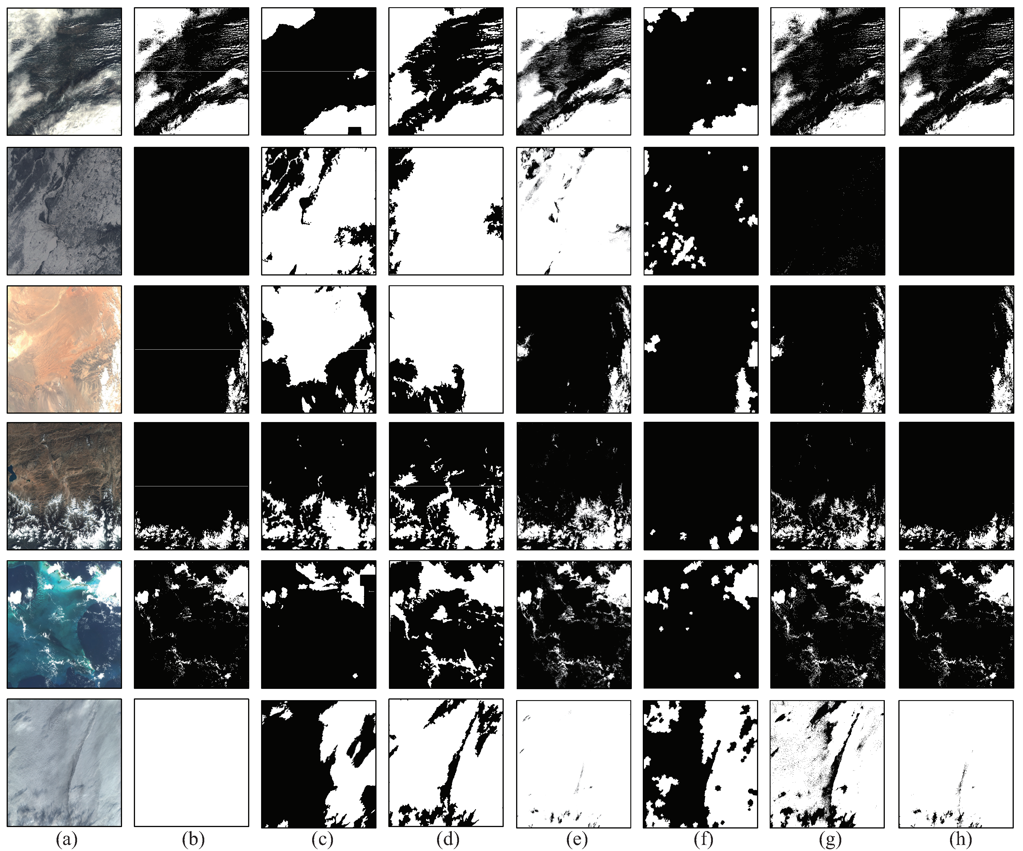
We conduct several groups of experiments to evaluate the performance of our proposed method. Before we conduct these experiments, we collect a challenging dataset with 502 GF-1 WFV images, which contains different land features such as ice, snow, desert, sea and vegetation and the dataset is the largest cloud dataset to the best of our knowledge, which is proper for the research in Big Data Era. First we evaluate the effectiveness of FECN, where we compare two different ways of utilizing multilevel feature information, Prediction Fusion and Feature Concatenation and we also compare different types of FECN. The experimental results show that Feature Concatenation is more effective and FECN_123457 performs better. Further, we examine multiple types of MWGF, where the filter with both small and large window sizes can refine the cloud probability map better. Finally, we compare our method with physical methods, physical methods integrated with statistical techniques and other deep learning methods, where our method outperforms others. Therefore, all these experimental results indicate that our method, which utilizes multilevel features of the imagery, is an effective method of cloud detection.

In our future work, we will focus on improving the computational efficiency of the proposed cloud detection method. Meanwhile, the relationships of the features in the convolutional network will be investigated.