Article

Snow Cover Monitoring with Chinese Gaofen-4 PMS Imagery and the Restored Snow Index (RSI) Method: Case Studies

1
Institute of Remote Sensing and Geographic Information System, School of Earth and Space Sciences, Peking University, Beijing 100871, China
2
Engineering Research Center for Geographical Information Basic Software and Application, State Bureau of Surveying and Mapping, Beijing 100871, China
3
Beijing Key Laboratory of Spatial Information Integration and 3S Application, Peking University, Beijing 100871, China
*
Author to whom correspondence should be addressed.
Remote Sens. 2018, 10(12), 1871; https://doi.org/10.3390/rs10121871
Submission received: 19 September 2018 / Revised: 1 November 2018 / Accepted: 17 November 2018 / Published: 23 November 2018
(This article belongs to the Section Remote Sensing in Geology, Geomorphology and Hydrology)

Abstract

:
Snow cover is an essential climate variable of the Global Climate Observing System. Gaofen-4 (GF-4) is the first Chinese geostationary satellite to obtain optical imagery with high spatial and temporal resolution, which presents unique advantages in snow cover monitoring. However, the panchromatic and multispectral sensor (PMS) onboard GF-4 lacks the shortwave infrared (SWIR) band, which is crucial for snow cover detection. To reach the potential of GF-4 PMS in snow cover monitoring, this study developed a novel method termed the restored snow index (RSI). The SWIR reflectance of snow cover is restored firstly, and then the RSI is calculated with the restored reflectance. The distribution of snow cover can be mapped with a threshold, which should be adjusted according to actual situations. The RSI was validated using two pairs of GF-4 PMS and Landsat-8 Operational Land Imager images. The validation results show that the RSI can effectively map the distribution of snow cover in these cases, and all of the classification accuracies are above 95%. Signal saturation slightly affects PMS images, but cloud contamination is an important limiting factor. Therefore, we propose that the RSI is an efficient method for monitoring snow cover from GF-4 PMS imagery without requiring the SWIR reflectance.

Graphical Abstract

1. Introduction

Snow is an important type of land cover. During the northern hemisphere winter, approximately one-third of the global land surface can be covered by snow [1,2]. Seasonal variation characteristics owing to extensive snowfall in winter and rapid snowmelt in spring make snow a significantly dynamic component of the ecosystem [2,3]. Snow plays a key role in the heat exchange and energy balance between the atmosphere and land surface because of its high albedo in visible and near-infrared (VNIR) bands [1,4,5]. Hence, snow cover has been selected as one of the essential climate variables of the Global Climate Observing System [6]. Moreover, more than half of the global fresh water is in solid form [5,7,8]. Seasonal snowmelt runoff is a major source of water for humans and ecosystems in mid–high latitudes and mountainous areas [1,9,10,11,12,13]. The long duration of snowfall in winter can lead to snow disasters, whereas the rapid snowmelt in spring can result in flooding hazards [14,15]. Therefore, monitoring snow cover is essential for climate change study, water resource management, and disaster prevention and mitigation.
Monitoring snow cover with in situ data is difficult due to the large extent, complex terrain, and remoteness of snow-covered areas [3,4,16]. Remote sensing provides a more practical means to monitor snow cover than using in situ data. Distribution of snow-covered areas is a crucial component of information about snow cover. Optical remote sensing data have been used to map snow cover distribution since 1960 [1]. The original methods fully utilize the high reflectance of snow in VNIR bands to detect snow cover with thresholds. However, the detection results are often mixed with clouds, deserts, and other land cover types with high reflectance. To address this limitation, snow index methods have been proposed on the basis of the fact that the reflectance of snow in the shortwave infrared (SWIR) band is low [5,17,18]. The normalized difference snow index (NDSI) is the most widely used snow index method, which combines the reflectance in the green and SWIR bands to enhance the spectral signature of snow [5]. Hall et al. constructed an algorithm called “SNOWMAP” on the basis of the NDSI, and this algorithm can automatically generate global snow cover datasets from the Moderate Resolution Imaging Spectroradiometer (MODIS) data [19,20,21]. Apart from snow cover detection, the NDSI value is also related to certain characteristics of snow cover, such as subpixel fractional snow cover [22,23]. Shimamura et al. also developed a snow index called “S3” and successfully applied it to snow cover monitoring in Japan [24]. Supervised and unsupervised classification methods can also detect snow cover. However, the classification results are usually binary, which provide less information of snow cover than results of snow index methods.
Many optical remote sensing sensors, such as the Thematic Mapper (TM) [5], Enhanced Thematic Mapper Plus (ETM+) [25], Operational Land Imager (OLI) [25], Advanced Very High Resolution Radiometer (AVHRR) [26], MODIS [1], and Visible Infrared Imaging Radiometer Suite (VIIRS) [1], have provided data for snow cover monitoring over the past 50 years. Spatial resolutions of remote sensing data from the TM, ETM+, OLI, and other similar sensors are relatively high and can thus provide detailed snow cover distribution. However, temporal resolutions of these data are relatively low, thereby limiting the capability of dynamic snow cover monitoring. As for data from the AVHRR, MODIS, VIIRS, and other similar sensors, their advantages and disadvantages are simply the opposite. The panchromatic and multispectral sensor (PMS) onboard the Chinese satellite Gaofen-4 (GF-4) can obtain remote sensing image in VNIR bands with 50-m spatial resolution at nadir and flexible temporal resolution [27,28]. These images present unique advantages in snow cover monitoring. GF-4 is a geostationary orbit optical remote sensing satellite and is the fourth satellite in the Chinese high-definition Earth observation system [29,30]. The spatial resolution of the GF-4 PMS imagery is much higher than those of other geostationary satellite data. Furthermore, GF-4 can conduct multiple observations of China and its surrounding areas within one day or continuous observation of specific regions with up-to-the-minute frequency. To date, no similar optical remote sensing data are available elsewhere in the world. However, the GF-4 PMS lacks the SWIR band centered near 1.6 μm. To the best of our knowledge, no existing snow index is suitable for GF-4 PMS imagery. Therefore, we need to construct a new snow index to realize the potential of GF-4 PMS imagery in snow cover monitoring.
In this paper, we proposed a novel method termed the restored snow index (RSI) for snow cover monitoring from GF-4 PMS imagery. The proposed method can restore the reflectance of snow cover in the SWIR band with other reflectance data in the VNIR bands of the GF-4 PMS. The RSI was defined with the linear discriminant analysis (LDA) method and calculated with the restored SWIR reflectance. Distributions of snow cover can be mapped with a proper segmentation threshold applied to the RSI results. The RSI method was validated using two pairs of GF-4 PMS and Landsat-8 OLI images. The effectiveness of snow cover detection with RSI was verified in these cases. Furthermore, the RSI was designed as a method that does not require the reflectance in the SWIR band for snow cover monitoring from the GF-4 PMS imagery, and thus can be a reference for other remote sensing sensors that lack the SWIR band.

2. Data Source

2.1. GF-4 PMS Images

The China Center for Resources Satellite Data and Application (CCRSDA) provided the Level-1A GF-4 PMS data without atmospheric correction. The original GF-4 PMS images were transformed from digital number to top-of-atmosphere (TOA) radiance by using the radiometric calibration coefficients published on the official website of the CCRSDA [30]. Then, the TOA radiance images were atmospherically corrected to surface reflectance with a look-up table built by the Second Simulation of the Satellite Signal in the Solar Spectrum (6S) model. The surface reflectance images were geometrically corrected using the rational polynomial coefficient orthorectification [31]. Two scenes of GF-4 PMS images were obtained and processed to validate the effectiveness of the RSI method for snow cover monitoring.

2.2. Landsat-8 OLI Images

The OLI onboard the Landsat-8 satellite is a multispectral optical sensor and possesses the SWIR band and other existing bands on the GF-4 PMS. The NDSI has been successfully applied to the Landsat-8 OLI images [32,33]. The Landsat-8 surface reflectance higher level science data products are topographically and atmospherically corrected and can be ordered from the United States Geological Survey (USGS) Earth Resources Observation and Science Center Science Processing Architecture On-Demand Interface. In this study, the Landsat-8 OLI images were used to build the RSI method as a substitution of the GF-4 PMS images and to evaluate the relationship and differences between the RSI and NDSI.
For building the RSI method, we obtained nine scenes of the Landsat-8 surface reflectance higher level science data products. Considering varying conditions, such as snow cover types, land cover types of background, data acquisition dates, and topographies, the nine OLI images were distributed in different parts of the observation areas of the GF-4. Figure 1 shows the location of these images and the corresponding paths and rows. Snow cover pixels in the nine OLI images were detected by a NDSI threshold of 0.4 and a reflectance threshold of 0.11 in the near-infrared (NIR) band, as proposed by Riggs et al. [19]. After the snow cover detection, a sample of 180,000 pixels, which comprised 10,000 snow cover pixels and 10,000 background pixels per image, was selected randomly for the following research.
For evaluating the relationship and differences between the RSI and NDSI, we obtained two scenes of the Landsat-8 surface reflectance higher level science data products. The coverage of these Landsat-8 OLI images was the same as the coverage of the previous GF-4 PMS images. The OLI images were upscaled from 30 m to 50 m to match the spatial resolution of the PMS images by using the pixel aggregate method [34]. Then, the PMS and OLI images were registered on the basis of the ground control points that were manually selected. The two pairs of the PMS and OLI surface reflectance images were used in the following validation.

3. Methodology

3.1. Spectral Matching between PMS and OLI

The reflectance of snow cover in the SWIR band is low [5,17,18], which is one of the most important features used to construct snow index methods. Therefore, the RSI was designed to take advantage of this feature. Considering the absence of the SWIR band on the GF-4 PMS, a SWIR band restoration method for GF-4 PMS needed to be constructed by indirectly using other appropriate remote sensing data. As mentioned previously, the Landsat-8 OLI images were selected as a substitution for the GF-4 PMS images to build the restoration method.
It was necessary to conduct spectral matching because of the differences between sensor parameters, such as the spectral responses of GF-4 PMS and Landsat-8 OLI in the corresponding bands. Table 1 and Figure 2 show the sensor parameters and spectral response functions of GF-4 PMS and Landsat-8 OLI [30,35,36]. The wavelength ranges of PMS are slightly wider than those of OLI in the visible bands. As for the NIR band, the wavelength range of PMS is much wider than that of OLI. The central wavelengths of PMS are close to those of OLI in the visible bands. As for the NIR band, the central wavelength of PMS is shorter than that of OLI. Furthermore, the spatial resolution of PMS is 1.6 times that of OLI.
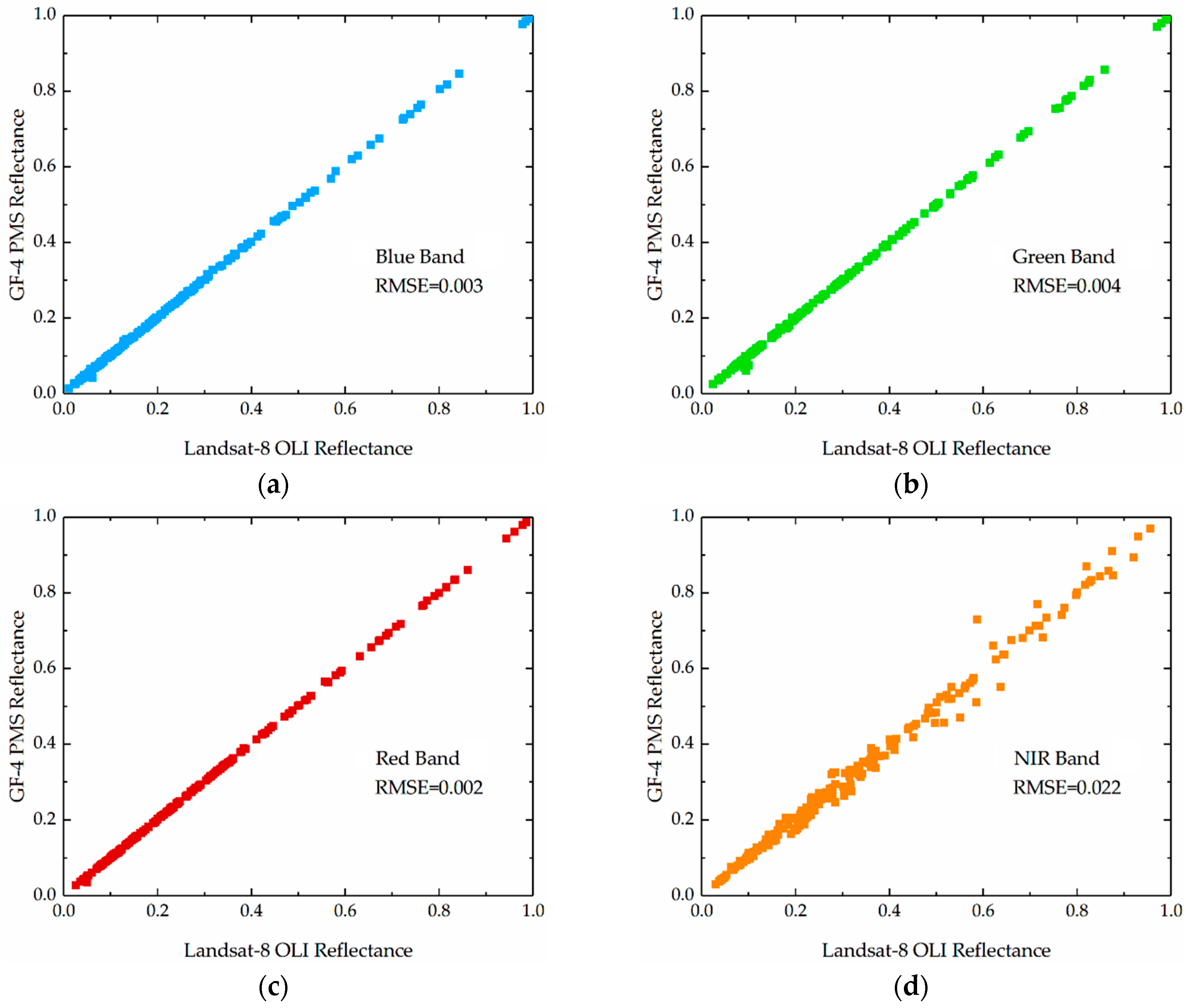
Considering the abovementioned differences, the differences in reflectance of the same objects between the two sensors in the corresponding bands need to be evaluated to ensure that the restoration method built with the OLI image also applies to the PMS image. The Johns Hopkins University Spectral Library [37] and the spectral response function of PMS and OLI were used to simulate the reflectance of typical objects in specific bands by using Equation (1):
R = λ 1 λ 2 R λ × SPF λ d λ
where R is the reflectance in the band; R λ is the reflectance at the wavelength; SPF λ is the normalized spectral response at the wavelength; and λ 1 and λ 2 are the initial and end wavelengths of the band, respectively. The reflectance of 214 typical objects such as igneous rocks, manmade materials, metamorphic rocks, sedimentary rocks, snow, soil, and vegetation were calculated. Figure 3 shows the scatterplots of the GF-4 PMS reflectance versus the Landsat-8 OLI reflectance. The consistency of reflectance of the same objects between the two sensors is very satisfactory in the visible bands. For the NIR band, the scatterplot exhibits greater variability from the trend line than those of the visible bands, and the root mean square error (RMSE) is an order of magnitude larger than those of the visible bands. This is mainly caused by the larger difference between the spectral response function of PMS and that of OLI in the NIR band. The NIR band of PMS is much wider and the central wavelength is shorter than that of OLI. If the reflectance of an object changes sharply in the wavelength range of 700 to 900 nm, such as for vegetation, the NIR reflectance of this object in PMS and OLI images will be different. However, the Landsat-8 OLI data are still a good substitution, considering the excellent consistency of the linear trend of PMS and OLI in the visible bands and the acceptable consistency of the linear trend in the NIR band.

3.2. Restoration of Reflectance of Snow Cover in the SWIR Band

For multispectral sensors, the reflectance in VNIR bands carry sufficient information to accurately restore the reflectance in the SWIR band [38]. Gladkova et al. successfully restored the partly nonfunctional band 6 (centered at 1.6 μm) data of the MODIS on Aqua with the quantitative image restoration (QIR) method based on multilinear regression [38,39]. Then, the restored data of band 6 are applied to calculate the NDSI and generate the MODIS Collection 6 snow cover products [1,39], which can be a reference for the restoration and RSI method for the GF-4 PMS.

3.2.1. Clustering and Regression

The QIR method is based on a multilinear regression using the information in a spatial–spectral window around each restored pixel [38,39]. The coefficients of multilinear regression are trained with data from the working detectors and are variational for each MODIS image. For the GF-4 PMS, there is no SWIR band data for training variational regression coefficients for each image. Fixed coefficients of multilinear regression may not apply to all observation areas of the GF-4. To evaluate the variability of regression coefficients, we trained the coefficients of multilinear regression with the abovementioned snow cover samples per OLI image. The reflectance of snow cover in blue, green, red, and NIR bands were used as the independent variables, and the reflectance of snow cover in the SWIR band was used as the dependent variable. The coefficients per image are shown in Table 2. Except for the intercept, the remaining coefficients of multilinear regression show great variability, which indicates the poor robustness of fixed regression coefficients.
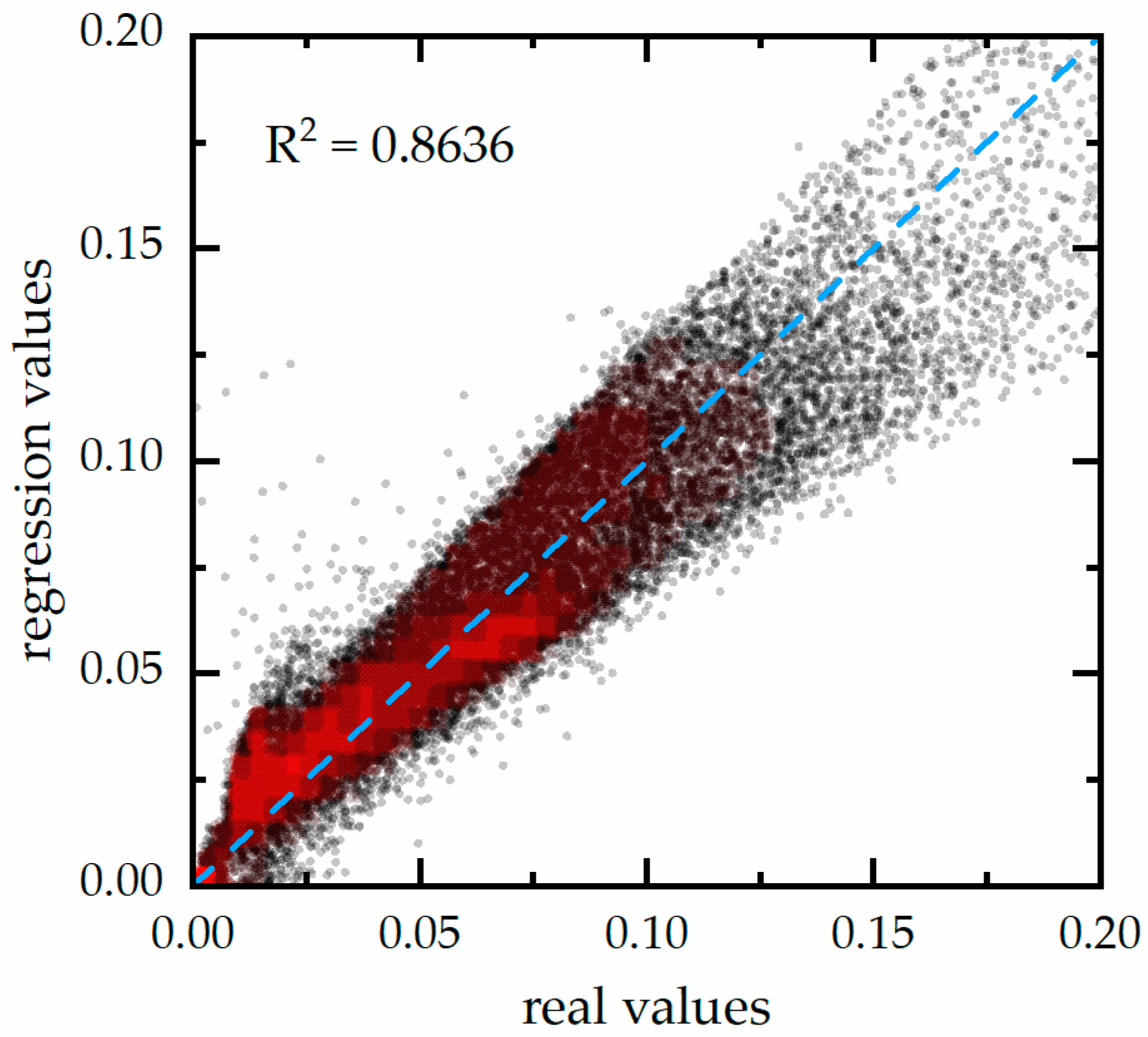
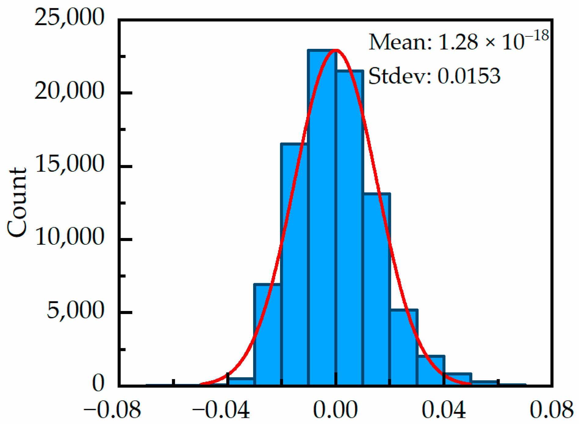
To reduce the influence of the variability of regression coefficients, unsupervised clustering was conducted before multilinear regression. The normalized difference between the reflectance in red and SWIR bands, as well as that between the reflectance in NIR and SWIR bands, was selected as the input feature of unsupervised clustering. The k-means clustering method was used as the unsupervised clustering algorithm [40]. After clustering, the regression coefficients were determined with the snow cover samples per cluster. The reflectance of snow cover in red and NIR bands were used as the independent variables, according to the better performance compared to other combinations of independent variables. The number of clusters needs to be determined before clustering, and was set to three in this study to balance the accuracy and complexity of the restoration method. Table 3 shows the cluster centers and regression coefficients per cluster. Figure 4 shows the scatterplot of the regression values versus the real values of the reflectance of the abovementioned snow cover samples in the SWIR band, and Figure 5 shows the histogram of the differences between the regression and real values of the SWIR reflectance of these samples. There is a slight nonlinear relationship between the regression and real values of the reflectance of these samples in the SWIR band. A proportion of the low values were overestimated, and a proportion of the high values were underestimated. Most of the scatter points are distributed near the 1:1 line, and the R 2 value is 0.8636. Moreover, the distribution of the differences is close to the normal distribution, with a mean close to zero, and the standard deviation is 0.0153, which indicate the satisfactory performance of the multilinear regression after unsupervised clustering.

3.2.2. Classification and Restoration

The normalized difference between the reflectance in the red and SWIR bands, as well as that between the reflectance in the NIR and SWIR bands, was used as the input feature of unsupervised clustering in this study. For GF-4 PMS images, there is no SWIR band available for calculating the normalized difference, thus the snow cover pixels cannot be classified with the previous clustering method. To determine the category of the snow cover pixels in GF-4 PMS images, a multilayer feedforward neural network was trained as the supervised classifier with the previous results of the unsupervised clustering. Figure 6 shows the structure of the neural network, which contains two hidden layers. The first hidden layer contains twelve neurons, and the second hidden layer contains nine neurons. The network was trained using the Bayesian regulation backpropagation algorithm [41]. The input of the network is the reflectance of snow cover in the blue, red, green, and NIR bands, and the output is the probability that the snow cover belongs to each cluster.
After the supervised classification, the restored reflectance of snow cover in the SWIR band was calculated using Equation (2):
R S W I R r = i = 1 3 p i ( a i × R r e d + b i × R N I R + c i )
where R S W I R r is the restored reflectance of snow cover in the SWIR band; p i is the probability that the snow cover belongs to cluster i and i = 1 3 p i = 1 ; a i , b i , and c i are the regression coefficients and intercept of cluster i ; and R r e d and R N I R are the reflectance of snow cover in the red and NIR bands, respectively. According to the restoration process, the restored reflectance in the SWIR band is a complex nonlinear combination of the whole information provided by the reflectance in the VNIR bands, and the restoration method is only suitable for snow cover.
Figure 7 shows the scatterplot of the restored reflectance versus the real reflectance of the abovementioned snow cover samples in the SWIR band. The scatterplot exhibits greater variation and a stronger nonlinear trend compared to Figure 4, which is due to the fact that the supervised classification cannot completely reproduce the results of the unsupervised clustering. Figure 7 inherits and enhances the nonlinearity shown in Figure 4. This enhancement was mainly caused by the loss function adopted to train the neural network. The mean square error (MSE) of the restoration results was used as the loss function. The parameters of the neural network were optimized to minimize the value of the MSE during the training process. For low values, the errors of these samples are small and contribute little to the value of the MSE. For high values, the amount of these samples is small, and the contribution is also small. Therefore, the errors of samples with medium reflectance were optimized effectively to minimize the value of the MSE. However, the overestimation of low reflectance and estimation of high reflectance were not well suppressed, which led to the visible nonlinearity.
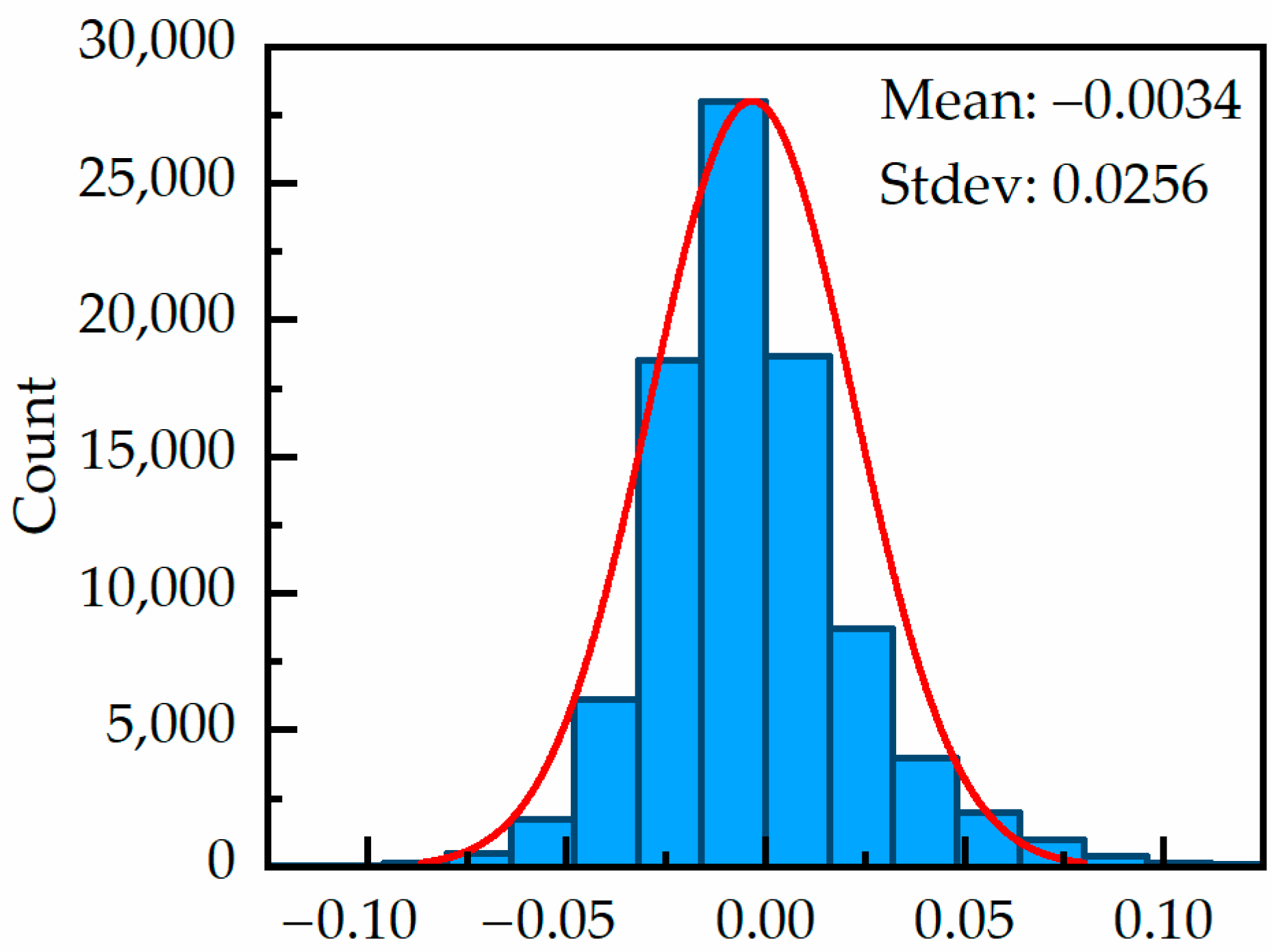
However, from the density distribution of the scatterplot shown in Figure 7, most of the scatter points are still distributed near the 1:1 line and the R 2 value is 0.6161. Figure 8 shows the histogram of the differences between the restored and real SWIR reflectance of these samples. The distribution of the differences is still close to the normal distribution, with a mean close to zero, and the standard deviation is 0.0256. This distribution of the differences indicates that the errors of most samples are close to zero, and there is almost no overall systematic error in the restoration results.

3.3. Restored Snow Index

The NDSI is defined as the normalized difference between the reflectance in the green and SWIR bands. For snow cover, the reflectance in the green band is higher than that in the SWIR band. The NDSI value of snow cover is positive, whereas those of other land cover types are negative or close to zero. Therefore, the NDSI can separate snow cover and background by enhancing the spectral signature of snow cover. For GF-4 PMS images, we have already built the restoration method to restore the reflectance of snow cover in the SWIR band. After the restoration, the NDSI can be calculated as follows:
N D S I r = R g r e e n R S W I R r R g r e e n + R S W I R r
where R g r e e n is the reflectance in the green band, R S W I R r is the restored reflectance in the SWIR band, and N D S I r is the NDSI calculated with the restored SWIR reflectance.
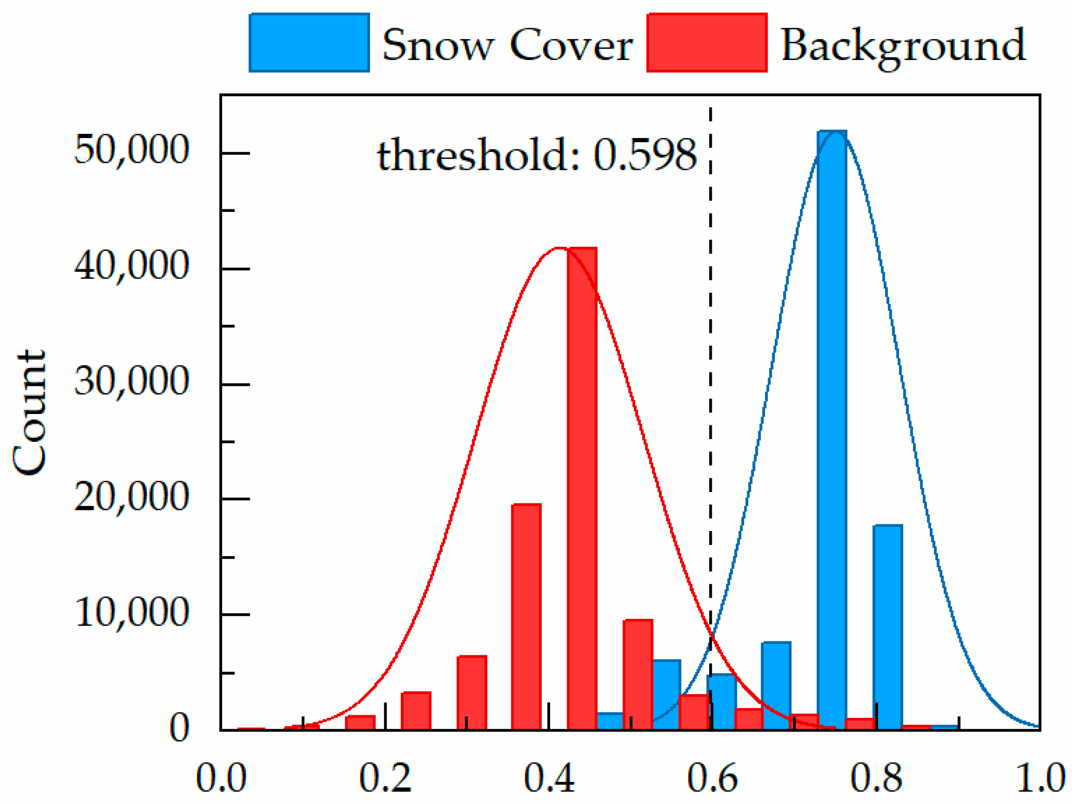
However, the restoration method is built with snow cover samples and is unsuitable for other land cover types. The restored SWIR reflectance of snow cover is accurate, but those of other land cover types may be not. Therefore, the effectiveness of the N D S I r for snow cover detection may be weakened. To evaluate the effectiveness of the N D S I r , the abovementioned snow cover and background samples from nine OLI images were used to restore the SWIR reflectance and calculate the N D S I r . Figure 9 illustrates the histograms of the N D S I r value of the 90,000 snow cover and 90,000 background pixels.
As shown in Figure 9, the separability between the N D S I r value of snow cover and that of background is weakened. The N D S I r value of snow cover is still positive, but that of the background is positive too. Most of the snow cover and background samples can be distinguished by differences in the N D S I r value. The overall accuracy of classification can reach 93.28% when the segmentation threshold is set to 0.598, but there are still 4.78% of the snow cover samples and 8.67% of the background samples misclassified with the optimal segmentation threshold, which is unsatisfactory.
To enhance the separability of the snow cover and background and take advantage of the restored SWIR reflectance of snow cover, the RSI was built with the LDA method, which has been widely used to construct classification-oriented multispectral indices [42,43]. The LDA is a method that can find a linear combination of multiple variables and aims to enhance the separability between different categories. The resulting combination can be used as a form of classification-oriented multispectral index [44].
Considering the spectral characteristics in VNIR bands and interaction between bands, the reflectance in the VNIR bands, the restored SWIR reflectance, and the N D S I r value of each pixel are seen as a six-dimensional vector for the GF-4 PMS image. The LDA method can obtain a transformation of the six-dimensional vectors by projecting the vectors onto a one-dimensional line. The separability between the snow cover and background was maximized after the projection. The abovementioned snow cover and background samples from nine OLI images were used as the training data for the LDA. The form of the RSI built with LDA is as follows:
R S I = 0.12 × R b l u e + 0.25 × R g r e e n + 0.01 × R r e d 0.32 × R N I R + 0.90 × R S W I R r + 0.09 × N D S I r
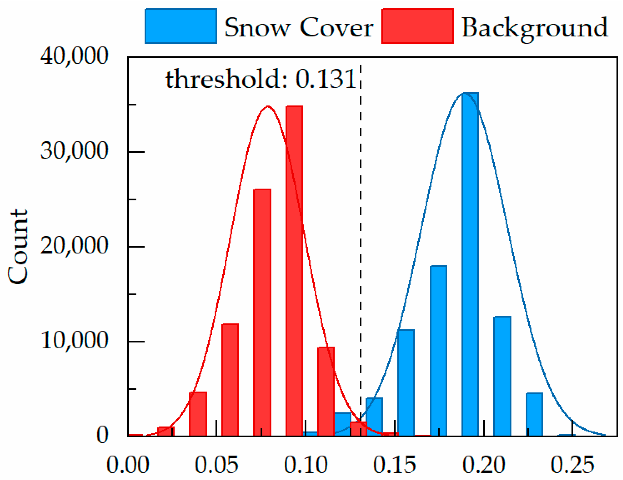
where R b l u e , R g r e e n , R r e d , and R N I R are the reflectance in the VNIR bands, respectively; R S W I R r is the restored reflectance in the SWIR band; and N D S I r is the NDSI calculated with the restored SWIR reflectance. The abovementioned snow cover and background samples from nine OLI images were used to calculated the RSI. Figure 10 illustrates the histograms of the RSI values of the 90,000 snow cover and 90,000 background pixels.
The separability between the snow cover and background is enhanced. The overall accuracy of classification can reach 98.34% when the segmentation threshold is set to 0.131. Overall, 2.67% of the snow cover samples and 0.64% of the background samples are misclassified with the optimal segmentation threshold, which is more satisfactory than the performance of the N D S I r .
As mentioned previously, the restored SWIR reflectance, as well as the N D S I r , is not a simple linear combination of the reflectance in VNIR bands. By introducing these nonlinear combinations into the RSI, the performance of the classification could be improved. As a comparison, the best overall accuracy of classification is 97.75%, using a simple VNIR-band linear classifier trained with the LDA method, which is lower than that of the RSI.
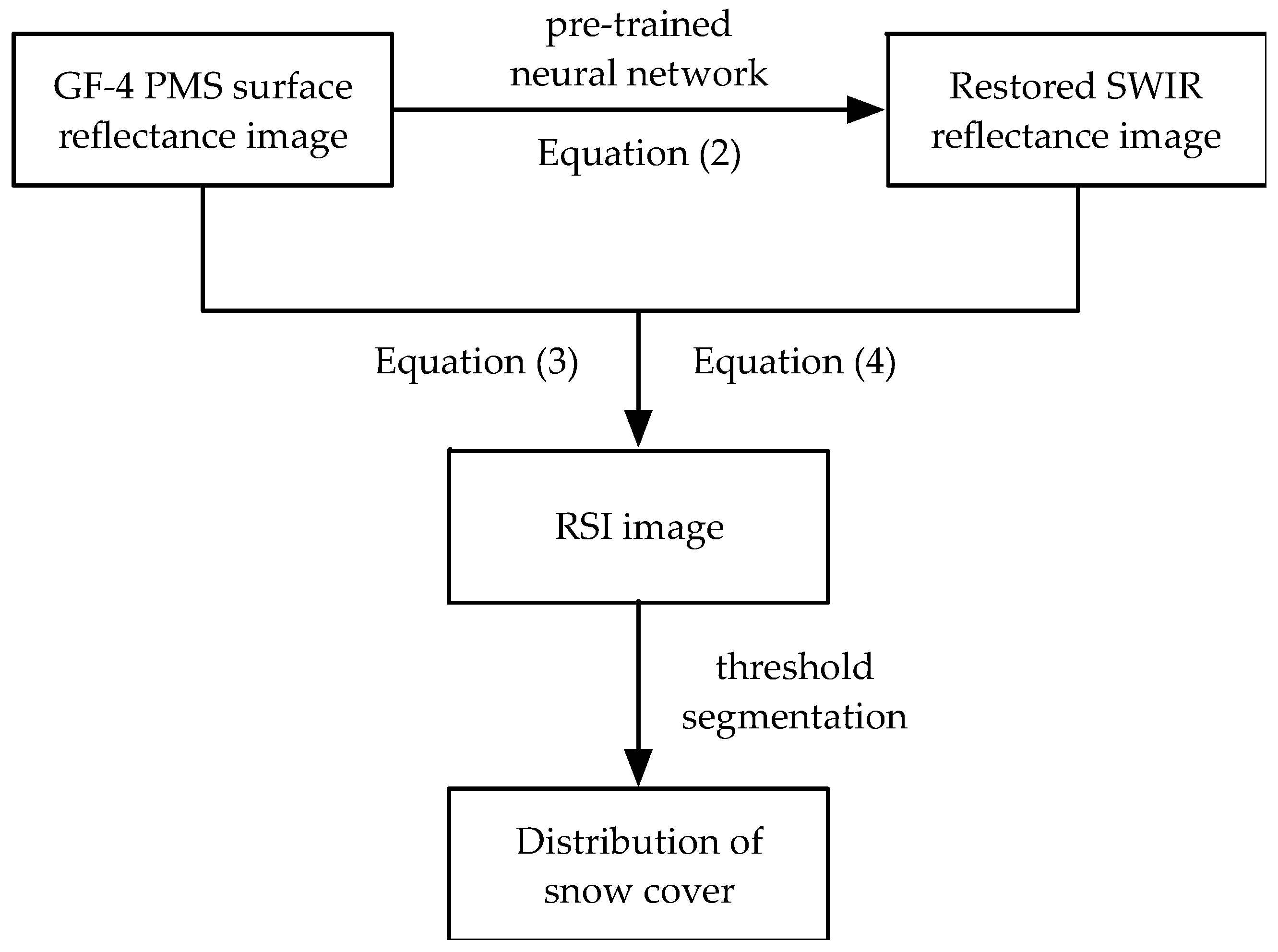
In summary, the RSI method for snow cover monitoring from GF-4 PMS imagery can be summarized as three steps. First, the SWIR reflectance of pixels in GF-4 PMS surface reflectance images are restored with the pretrained multilayer feedforward neural network and Equation (2). Then, the RSI values are calculated with the Equations (3) and (4), which provide more information of snow cover than binary classification results. Finally, the distribution of snow cover can be mapped with a proper segmentation threshold applied to the RSI image. Figure 11 presents the flowchart of the proposed RSI method.

4. Validation

4.1. Test Sites

To validate the efficiency of the RSI method, we selected two test sites after taking the representativeness of the snow cover samples and availability of the remote sensing data into consideration. The first test site is located in Chengde City, Hebei Province, northeastern China, and the second one is located in Qinghai Province, northwestern China, near the Hala Lake. As mentioned previously, a pair of the GF-4 PMS and Landsat-8 OLI images was obtained for each test site.
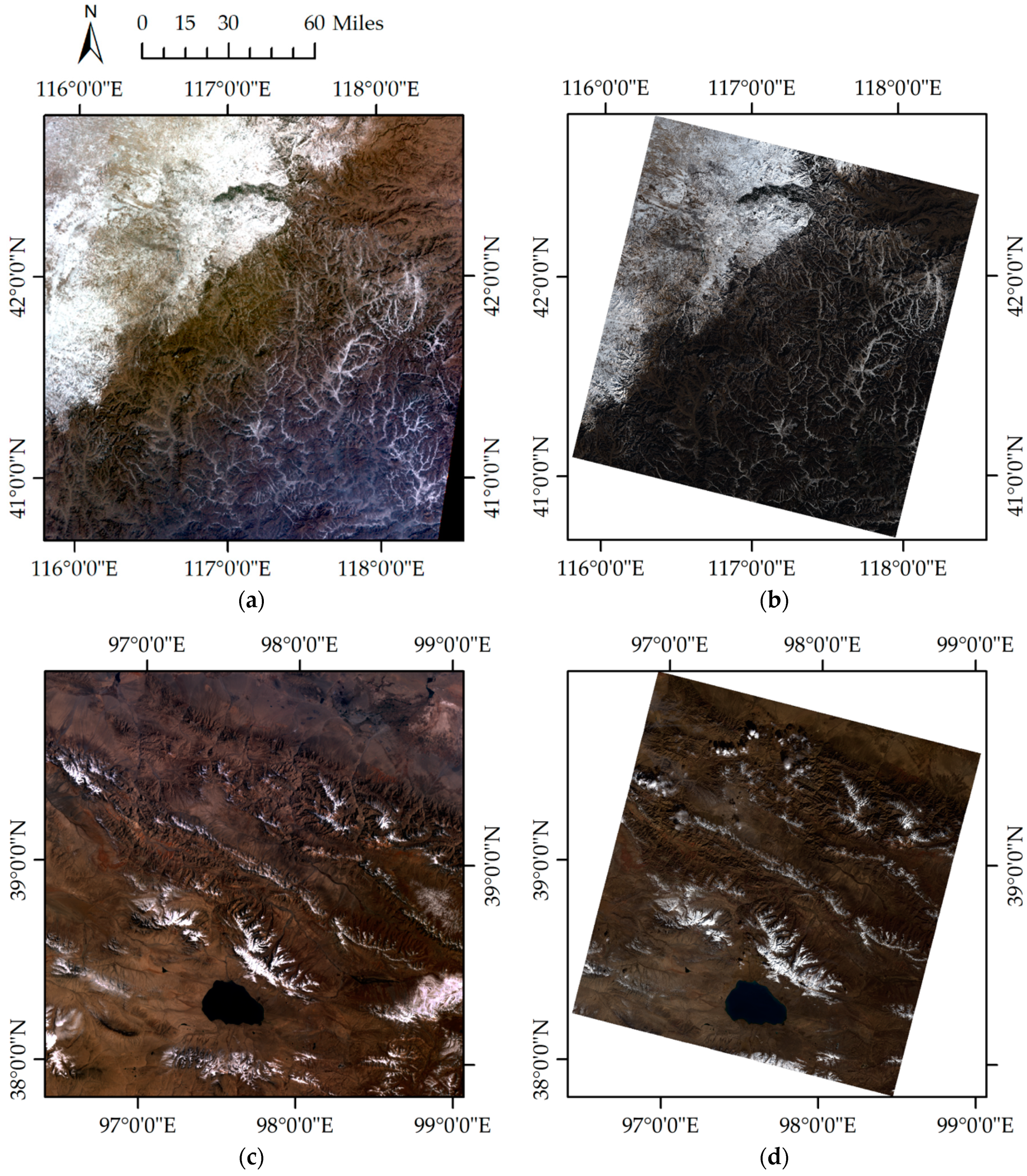
Figure 12 displays the green–red–blue (RGB) composite images of the overlapping regions between the PMS and OLI images. Table 4 presents the details of the two image pairs. The acquisition dates of the selected PMS and OLI images are as close as possible for each pair to reduce the temporal changes of snow cover and other land cover types. A snowfall occurred in the first test site on 12 December 2016. Most of the snow cover in the first test site belonged to the category of fine snow, as well as seasonal snow. No snowfall had occurred in the second test site before 15 October 2016. Most of the snow cover in the second test site belonged to the categories of medium and coarse granular snow, as well as perennial snow.

4.2. Results

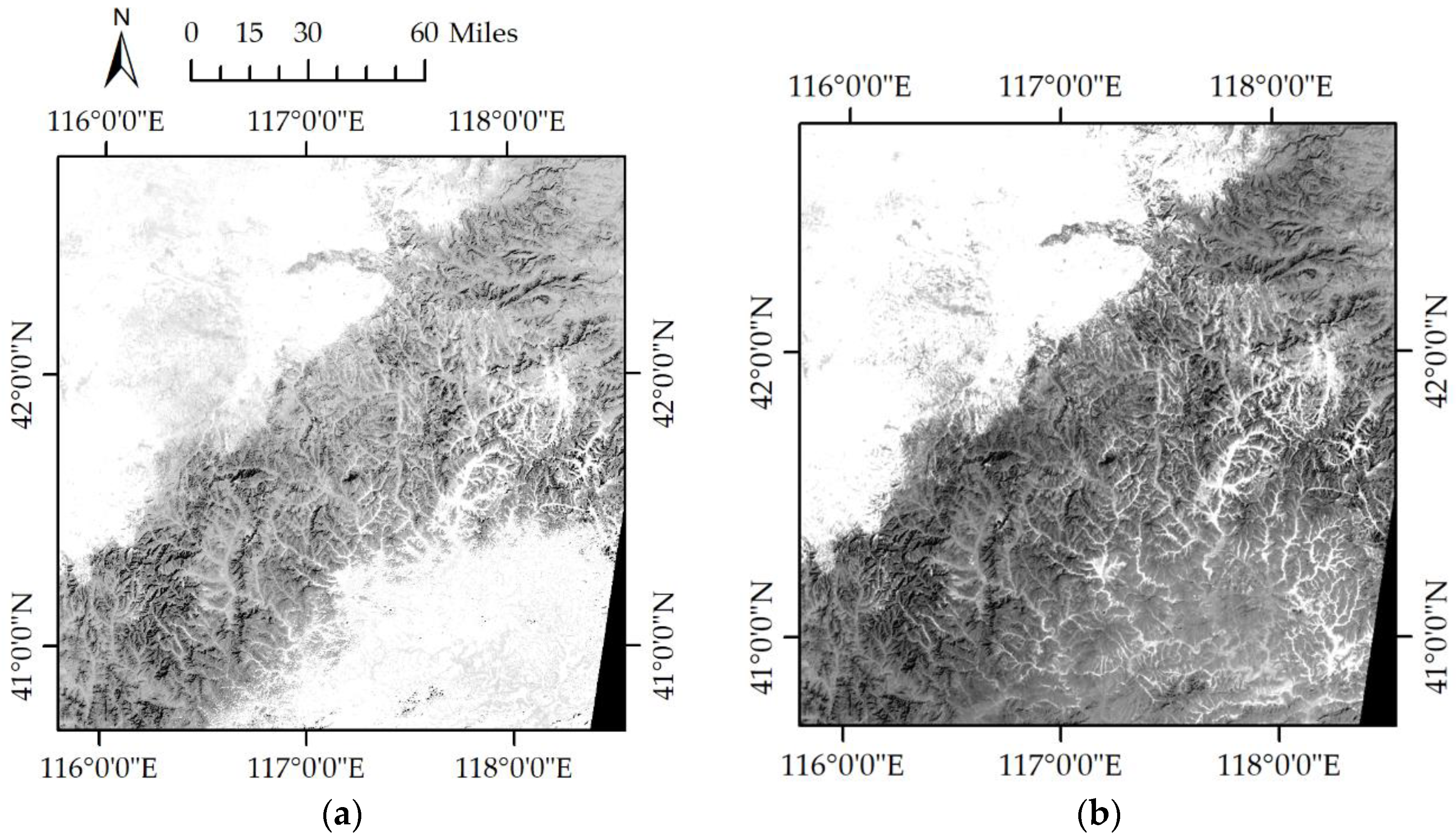
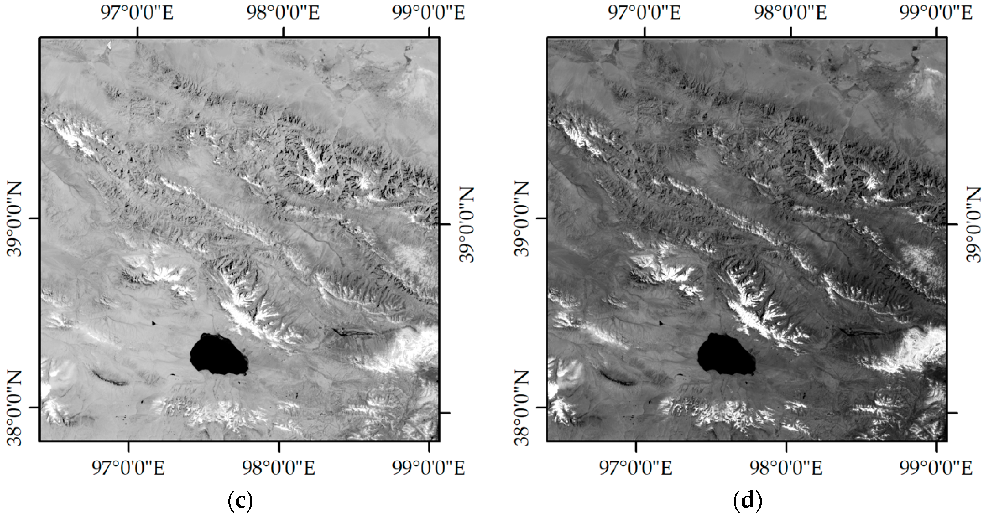
The GF-4 PMS surface reflectance images were processed according to the flowchart shown in Figure 11. The SWIR reflectance images were restored, and then the N D S I r and RSI images were calculated. Figure 13 displays the N D S I r results and the RSI results of the two test sites, respectively. By comparing the N D S I r and RSI images, it can be found that the contrast between the snow cover and background is more significant in the RSI images than in the N D S I r images. The N D S I r cannot distinguish snow cover from bare land in the mountainous area in the southeast part of the first test site. For the RSI images, the contrast between snow cover and bare land in that area is more satisfactory, which indicates the necessity and effectiveness of the RSI method for snow cover monitoring from GF-4 PMS images.
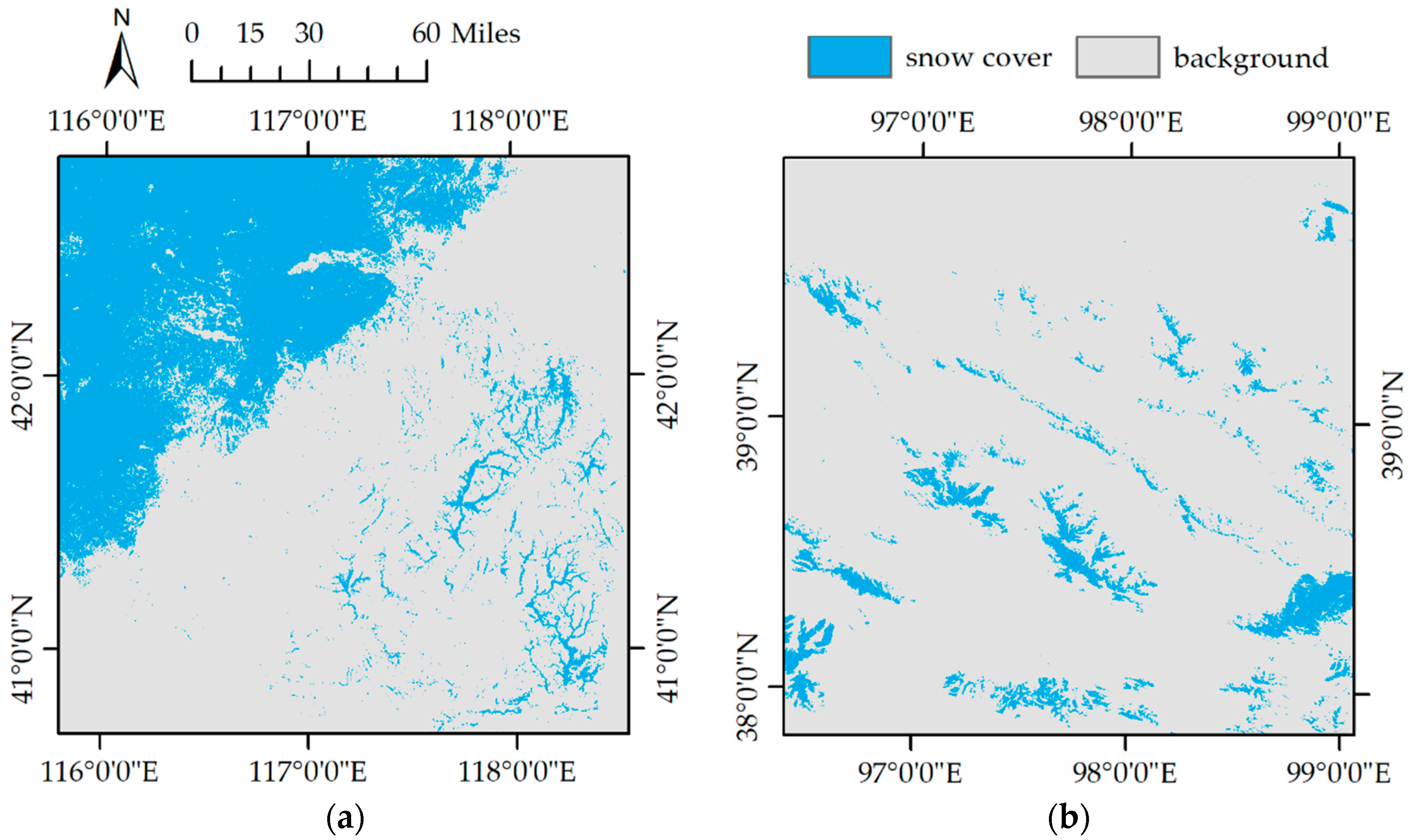
After calculating the RSI images, the distribution of snow cover of the two test sites were mapped with a segmentation threshold, which was set to 0.131 according to Section 3.3. Figure 14 displays the classification results. The blue part denotes the pixels that are classified as snow cover, while the gray part denotes the pixels that are classified as background. Fine snow in the first test site and medium and coarse snow in the second test site are successfully detected, which verifies the effectiveness of the RSI method when applied to the GF-4 PMS images in these cases. To quantitatively evaluate the classification accuracy, a sample of 10,000 pixels, which comprises 5000 pixels from the first test site and 5000 pixels from the second test site, was selected randomly and used as the validation dataset. To avoid subjective influence, the real categories of the samples were determined by visual interpretation one by one without knowing the classification results of the RSI method. The number of the snow cover pixels identified by visual interpretation is 3179. As for the background pixels, the number is 6821. We obtained a confusion matrix for the total of the 10,000 sample pixels. Table 5 calculates and lists the classification accuracies.
A total of 159 snow cover pixels are misclassified as background, while 42 background pixels are misclassified as snow cover. Most of the omission snow cover pixels occurred in the northwestern part of the first test site. There was a seven-day gap between the snowfall and acquisition dates of the GF-4 PMS images in the first test site. During the seven days, impurities, such as soils and ashes, polluted a certain part of the snow cover. The spectral characteristics of the polluted snow cover change to a certain extent, thereby resulting in the omission errors. Most of the commission snow cover pixels occurred in the eastern part of the second test site. The real categories of most commission pixels are cloud with high reflectance in VNIR bands. The spectral characteristics of clouds are similar to those of snow cover in VNIR bands, thereby resulting in the commission errors. Although certain polluted snow and cloud pixels may be misclassified, all of the classification accuracies of the snow cover identification are above 95%, which demonstrates the effectiveness of the RSI method when applied to cloud-free GF-4 PMS images in these cases.

4.3. Comparison between RSI and NDSI

As mentioned previously, the NDSI is the most widely used snow index method, which is adopted to generate most of the global and regional snow cover datasets [5,19,20,21]. Therefore, the relationship and difference between the RSI and NDSI need to be evaluated. According to the definitions of the RSI and NDSI, there is no simple linear relationship between the values of the RSI and NDSI. Due to the fact that the restored SWIR reflectance of land cover types other than snow cover may not be accurate, the N D S I r value cannot represent the real NDSI value. Therefore, the Landsat-8 OLI surface reflectance images were used to calculate the NDSI images.
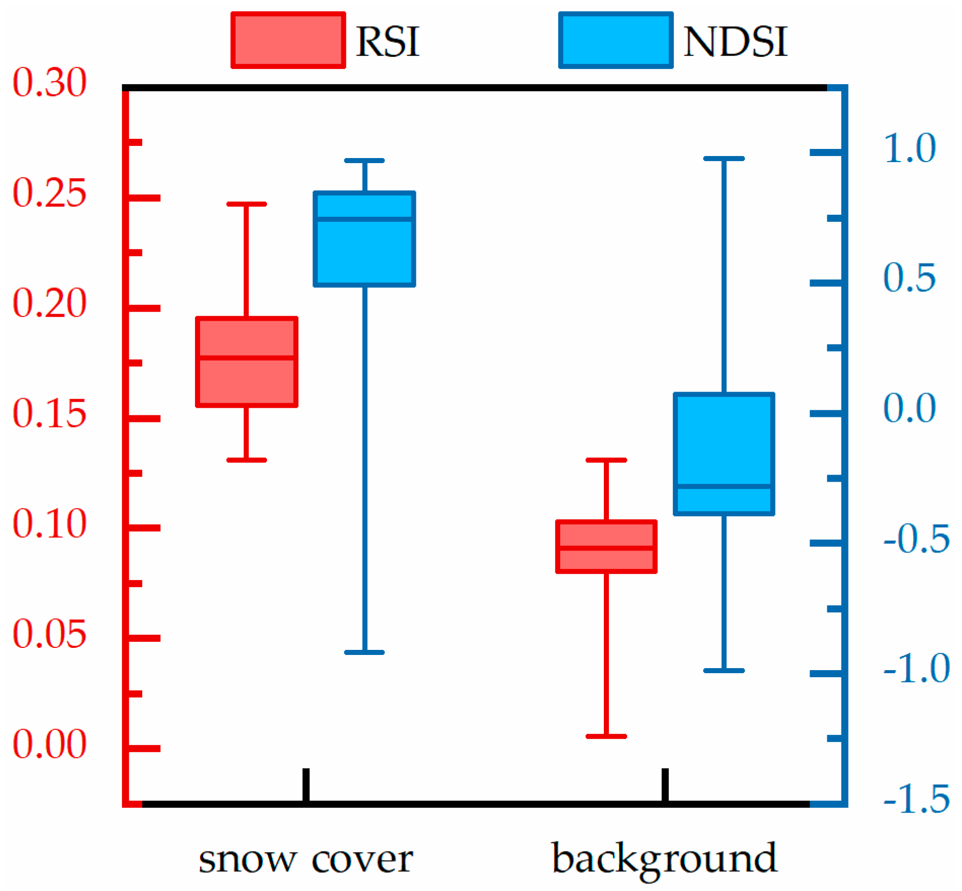
The distributions of the RSI and NDSI values of snow cover and background samples classified by the RSI method are shown in Figure 15 by the box and whisker plots. The RSI ranges from 0 to 0.25, and the NDSI ranges from −1 to 1. The range of the NDSI is larger than that of the RSI. Both the RSI and NDSI can distinguish snow cover from background with a proper segmentation threshold. For the NDSI, the threshold is near zero. For the RSI, the values of background samples are also positive, and the snow cover and background cannot be distinguished by the positive or negative sign of the RSI value. The recommended value of the segmentation threshold for the RSI is near 0.13, which should be adjusted according to actual situations.

5. Discussion

5.1. Signal Saturation

The efficiency of the RSI method for snow cover monitoring from GF-4 PMS images has been evaluated in Section 4.2. However, the radiation resolution of PMS may limit its capacity for snow cover observation. The radiation resolution of PMS is 10 bits, whereas that of Landsat-8 OLI is 12 bits. Signal saturation is likely to occur in the PMS image when the reflectance of snow cover is very high. The saturated pixels will still be classified as snow cover by the RSI method. However, signal saturation will affect the reflectance of snow cover and change the corresponding RSI value.
To study the influence of signal saturation in the PMS image, we identified saturation pixels in the two scenes of the original GF-4 PMS images. Each scene of the original GF-4 PMS image has 104,857,600 pixels. Table 6 lists the numbers of the saturation pixels of the two test sites. No saturation pixels exist in the green band. For the other bands, the number of saturation pixels is also very small. The radiation resolutions of PMS in VNIR bands are the same, and the reflectance of snow cover in VNIR bands are on the same order of magnitude. The integration time of PMS images adopted in this study is 20 s in the green band, while it is 30 s in the other bands. Therefore, the signal saturation is absent in the green band. For other bands, the proportions of saturation pixels are very small. Signal saturation slightly affects the GF-4 PMS images of the two test sites. Furthermore, the integration time of PMS is flexible and can be adjusted to reduce the influence of signal saturation.

5.2. Cloud Contamination

Apart from signal saturation, cloud contamination is also an important limiting factor of snow cover monitoring. GF-4 is a geostationary satellite with high temporal resolution. The observation mode and temporal resolution of PMS onboard GF-4 are flexible. In the starring mode, the frequency of continuous observations made by GF-4 of the same location can reach the minute level [45]. As a comparison, the temporal resolution of Landsat-8 OLI is 16 days. Therefore, GF-4 can adjust the imaging time to obtain cloudless observation of a specific location, which is impossible for polar-orbiting satellites. However, the size of scanning areas of GF-4 PMS is 400 km × 400 km, which is much wider than that of Landsat-8 OLI. Considering the size of scanning areas, cloud cover can be common in a PMS image. The impact of cloud contamination on the RSI method cannot be ignored and should be discussed.
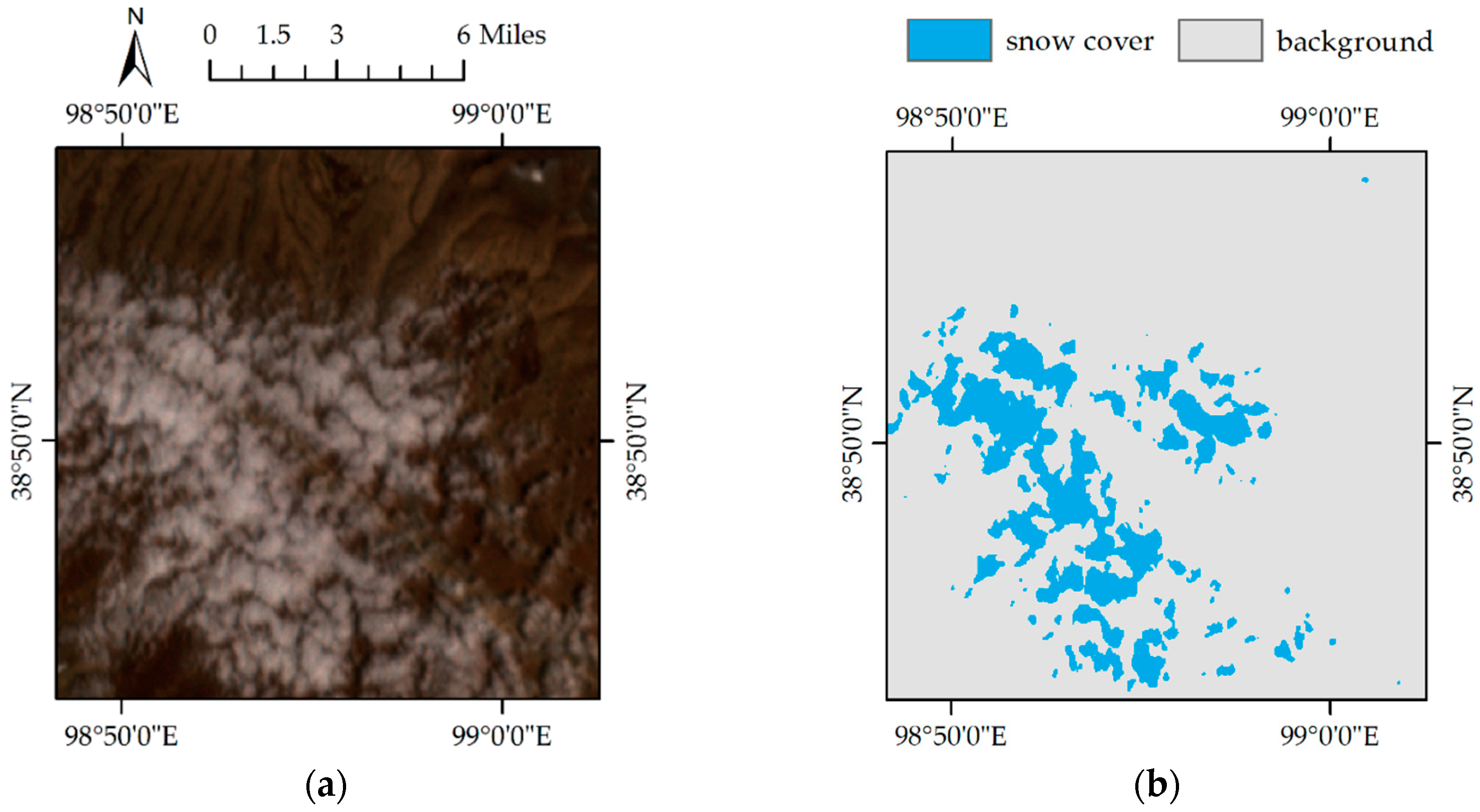
As mentioned previously, cloud pixels are the main cause of commission errors in snow cover detection. Figure 16 shows an enlarged view of the cloud pixels in the second test site. Thin clouds can be removed using the RSI method. Most of the thick clouds are misclassified as snow cover. The spectral signal of the land cover under the thin clouds can be partially captured by the sensor, thereby helping in removing the thin clouds. For thick clouds, the sensor does not capture the land cover signal. The spectral characteristics of thick clouds are very similar to those of snow cover in VNIR bands. Reflectance in the SWIR band can effectively separate the cloud and snow cover. However, GF-4 PMS lacks the SWIR band. Furthermore, the restoration of reflectance in the SWIR band is only suitable for snow cover. Therefore, the capability of GF-4 PMS image to distinguish thick clouds and snow cover is not as satisfactory as that of other remote sensing data comprising the SWIR band. The RSI method is only suitable for cloud-free parts of GF-4 PMS images, and accurate cloud masks are necessary for the RSI method when cloud contamination exists. Zheng et al. (in 2017) and Hu et al. (in 2018) independently constructed an automatic cloud detection algorithm for GF-4 PMS data [45,46]. Except for the spectral information, the morphological and texture features extracted from a single PMS image, as well as the temporal variations extracted from multitemporal PMS images, are used in their methods. By introducing additional information, the separation of cloud and other objects with high reflectance in VNIR bands is improved. The cloud masks generated by these cloud detection algorithms can be used for the preprocessing of PMS data and screening out cloud-free parts for the RSI method.
Furthermore, the GF-4 satellite possesses an infrared scanner (IRS) onboard. The GF-4 IRS images possess one middle infrared (MIR) band with wavelengths in the range of 3.5–4.1 μm. The reflectance of snow cover and cloud are different in the MIR band, which have been evaluated by Allen et al. [47]. The IRS image may be helpful in removing thick clouds. However, it is difficult to separate the reflectance from the MIR signal, and there is no such published algorithm for GF-4 IRS data so far. The brightness temperature could be a substitute for the reflectance in the MIR band for removing thick clouds [48]. However, the relative size of the temperature of cloud and snow cover is not stable, which may weaken the difference between the brightness temperature of cloud and snow cover. Therefore, the efficiency of removing thick clouds by using the GF-4 IRS images remains to be evaluated in future studies.

5.3. Limitations and Perspectives

The impacts of signal saturation and cloud contamination on the RSI method have been fully discussed previously. However, there are still other constraints that may limit the efficiency of the RSI method. Shadow is a significant limiting factor, especially for rugged topography. Without appropriate topographical correction, the reflectance of snow cover in shadows can be much lower than that of normal snow cover in VNIR bands, which may lead to misclassification. Furthermore, the tilt observation mode and flexible observation time of GF-4 could make shadow more common in GF-4 PMS data. Besides shadowing, the selection of the segmentation threshold is also important. An improper threshold value may result in unsatisfactory classification results. Considering the size of the scanning areas of GF-4 (400 km × 400 km), a single threshold may not be applicable to different parts of a scene of GF-4 PMS data.
The RSI method can map the distribution of snow cover without the SWIR reflectance and can be a reference for other similar remote sensing data without the SWIR band, such as the Wide Field Camera (WFV) data of GF-1, the Wide View CCD Camera (WVC) data of HJ-1, the High Resolution CCD Camera (HRCC) data of CBERS-1 and CBERS-2, and so on. However, the Landsat-8 OLI data were used as a substitution to build the RSI method. The consistency of the linear trend of OLI and PMS in VNIR bands were evaluated in this study. When applying the RSI method to other similar remote sensing data without the SWIR band, the consistency of the linear trend of OLI and other remote sensing sensor needs to be reevaluated. Differences in the spatial resolution, if they exist, also need to be addressed. It might not be wise to apply the RSI method directly to other similar remote sensing data. Nevertheless, the process and methodology of constructing the RSI method can provide a reference for building snow cover detection methods for other similar remote sensing sensors.
The RSI method was validated in two test sites, which were selected after taking the representativeness of multiple factors into consideration. However, further validation needs to be conducted to test the efficiency of the RSI method in different areas of the observation range of the GF-4. The RSI method was used to map the distribution of snow cover in this study. Just like other snow indices, the value of RSI may be related to some specific characteristics of snow cover, such as the fractional snow cover, snow grain size, and so on. This potential relationship between the RSI value and snow cover characteristics needs to be evaluated in the future studies to expand the application of the RSI method. The input of the RSI method is the surface reflectance, and therefore the precision of the surface reflectance will influence the performance of the RSI method. However, there is no published atmospheric correction algorithm for GF-4 PMS data as of yet. Constructing such atmospheric correction algorithms on the basis of the radiative transfer model or other theories will significantly strengthen the practicability of the RSI method.

6. Conclusions

Our study introduced a new method, termed the RSI, to monitor snow cover from GF-4 PMS imagery without the SWIR band. The reflectance of snow cover in the SWIR band is restored by comprehensively using unsupervised clustering, multilinear regression, and supervised classification. Based on the LDA method, the RSI are defined and calculated with the restored SWIR reflectance, which provides more information of snow cover than binary classification results. The distribution of snow cover can be mapped with a proper segmentation threshold applied to the RSI results.
The new method was applied to and validated with two pairs of GF-4 PMS and Landsat-8 OLI images. All of the classification accuracies of the snow cover detection were above 95%, which indicates the efficiency of the RSI method for snow cover detection in these cases. There is no simple linear relationship between the values of the RSI and NDSI, and the snow cover and background cannot be distinguished by the positive or negative sign of the RSI value. A proper segmentation threshold needs to determined and adjusted according to actual situations to map the distribution of snow cover. Although the radiation resolution of PMS is 10 bits, signal saturation slightly affects the PMS images used in this study, yet cloud contamination is still an important limiting factor of snow cover monitoring from PMS imagery.
The RSI method does not rely on SWIR reflectance and can thus be a reference to monitor snow cover from other remote sensing data without the SWIR band. This method is helpful in reaching the potential of GF-4 PMS imagery in snow cover monitoring.

Author Contributions

Conceptualization, H.R. and Q.Q.; Funding acquisition, Q.Q.; Methodology, T.Z. and H.R.; Validation, T.Z. and Y.S.; Visualization, T.Z. and Y.S.; Writing—original draft, T.Z.; Writing—review & editing, T.Z.

Funding

This work was supported by the National Key Research and Development Plan of China under Grant 2017YFB0503905-05, by the High Resolution Earth Observation System of the National Science and Technology Major Project of China under Grant 11-Y20A05-9001-15/16, and by the National Natural Science Foundation of China under Grants 41,771,371 and 51,709,003.

Acknowledgments

The authors appreciatively acknowledge the USGS for providing the Landsat-8 OLI data and the CCRSDA for providing the GF-4 PMS data. The authors also acknowledge Dr. Gongqi Zhou for providing the measured spectral reflectance data of snow cover, which were used in the previous analysis.

Conflicts of Interest

The authors declare no conflict of interest.

References

  1. Riggs, G.A.; Hall, D.K.; Román, M.O. Overview of NASA’s MODIS and Visible Infrared Imaging Radiometer Suite (VIIRS) snow-cover Earth System Data Records. Earth Syst. Sci. Data 2017, 9, 765–777. [Google Scholar] [CrossRef]
  2. Frei, A.; Tedesco, M.; Lee, S.; Foster, J.; Hall, D.K.; Kelly, R.; Robinson, D.A. A review of global satellite-derived snow products. Adv. Space Res. 2012, 50, 1007–1029. [Google Scholar] [CrossRef] [Green Version]
  3. Shreve, C.M.; Okin, G.S.; Painter, T.H. Indices for estimating fractional snow cover in the western Tibetan Plateau. J. Glaciol. 2009, 55, 737–745. [Google Scholar] [CrossRef] [Green Version]
  4. Dobreva, I.D.; Klein, A.G. Fractional snow cover mapping through artificial neural network analysis of MODIS surface reflectance. Remote Sens. Environ. 2011, 115, 3355–3366. [Google Scholar] [CrossRef] [Green Version]
  5. Dozier, J. Spectral signature of alpine snow cover from the Landsat Thematic Mapper. Remote Sens. Environ. 1989, 45, 9–22. [Google Scholar] [CrossRef]
  6. Bojinski, S.; Verstraete, M.; Peterson, T.C.; Richter, C.; Simmons, A.; Zemp, M. The Concept of Essential Climate Variables in Support of Climate Research, Applications, and Policy. B. Am. Meteorol. Soc. 2014, 95, 1431–1443. [Google Scholar] [CrossRef] [Green Version]
  7. Facts about Glaciers | National Snow and Ice Data Center. Available online: https://nsidc.org/cryosphere/glaciers/quickfacts.html (accessed on 7 October 2018).
  8. Ice and Glaciers -The Water Cycle-USGS Water-Science School. Available online: https://water.usgs.gov/edu/watercycleice.html (accessed on 7 October 2018).
  9. Dozier, J. Opportunities to improve hydrologic data. Rev. Geophys. 1992, 30, 315–331. [Google Scholar] [CrossRef]
  10. Douville, H.; Chauvin, F.; Planton, S.; Royer, J.F.; Salas-Mélia, D.; Tyteca, S. Sensitivity of the hydrological cycle to increasing amounts of greenhouse gases and aerosols. Clim. Dynam. 2002, 20, 45–68. [Google Scholar]
  11. Barnett, T.P.; Adam, J.C.; Lettenmaier, D.P. Potential impacts of a warming climate on water availability in snow-dominated regions. Nature 2005, 438, 303. [Google Scholar] [CrossRef] [PubMed]
  12. Bales, R.C.; Molotch, N.P.; Painter, T.H.; Dettinger, M.D.; Rice, R.; Dozier, J. Mountain hydrology of the western United States. Water Resour. Res. 2006, 42, W8432. [Google Scholar] [CrossRef]
  13. Painter, T.H.; Rittger, K.; Mckenzie, C.; Slaughter, P.; Davis, R.E.; Dozier, J. Retrieval of subpixel snow covered area, grain size, and albedo from MODIS. Remote Sens. Environ. 2009, 113, 868–879. [Google Scholar] [CrossRef] [Green Version]
  14. Rango, A. Spaceborne remote sensing for snow hydrology applications. Hydrolog. Sci. J. 1996, 41, 477–494. [Google Scholar] [CrossRef] [Green Version]
  15. Dobreva, I.D.; Klein, A.G. Fractional snow cover mapping through artificial neural network analysis of MODIS surface reflectance. Remote Sens. Environ. 2011, 115, 3355–3366. [Google Scholar] [CrossRef] [Green Version]
  16. Derksen, C.; Ledrew, E. Variability and change in terrestrial snow cover: Data acquisition and links to the atmosphere. Prog. Phys. Geog. 2000, 24, 469–498. [Google Scholar] [CrossRef]
  17. Nolin, A.W.; Liang, S. Progress in bidirectional reflectance modeling and applications for surface particulate media: Snow and soils. Remote Sens. Reviews 2000, 18, 307–342. [Google Scholar] [CrossRef]
  18. Singh, S.K.; Kulkarni, A.V.; Chaudhary, B.S. Hyperspectral analysis of snow reflectance to understand the effects of contamination and grain size. Ann. Glaciol. 2010, 51, 83–88. [Google Scholar] [CrossRef]
  19. Hall, D.K.; Riggs, G.A.; Salomonson, V.V. Development of Methods for Mapping Global Snow Cover Using Moderate Resolution Imaging Spectroradiometer Data. Remote Sens. Environ. 1995, 54, 127–140. [Google Scholar] [CrossRef]
  20. Hall, D.K.; Foster, J.L.; Verbyla, D.L.; Klein, A.G.; Benson, C.S. Assessment of Snow-Cover Mapping Accuracy in a Variety of Vegetation-Cover Densities in Central Alaska. Remote Sens. Environ. 1998, 66, 129–137. [Google Scholar] [CrossRef]
  21. Hall, D.K.; Riggs, G.A.; Salomonson, V.V.; Digirolamo, N.E.; Bayr, K.J. MODIS snow-cover products. Remote Sens. Environ. 2002, 83, 181–194. [Google Scholar] [CrossRef] [Green Version]
  22. Salomonson, V.V.; Appel, I. Estimating fractional snow cover from MODIS using the normalized difference snow index. Remote Sens. Environ. 2004, 89, 351–360. [Google Scholar] [CrossRef]
  23. Salomonson, V.; Appel, I. Development of the Aqua MODIS NDSI fractional snow cover algorithm and validation results. IEEE T. Geosci. Remote 2006, 44, 1747–1756. [Google Scholar] [CrossRef]
  24. Shimamura, Y.; Izumi, T.; Matsuyama, H. Evaluation of a useful method to identify snow-covered areas under vegetation-comparisons among a newly proposed snow index, normalized difference snow index, and visible reflectance. Int. J. Remote Sens. 2006, 27, 4867–4884. [Google Scholar] [CrossRef]
  25. Steele, C.; Dialesandro, J.; James, D.; Elias, E.; Rango, A.; Bleiweiss, M. Evaluating MODIS snow products for modelling snowmelt runoff: Case study of the Rio Grande headwaters. Int. J. Appl. Earth Obs. 2017, 63, 234–243. [Google Scholar] [CrossRef]
  26. Wang, S.; Yin, H.; Yang, Q.; Yin, H.; Wang, X.; Peng, Y.; Shen, M. Spatiotemporal patterns of snow cover retrieved from NOAA-AVHRR LTDR: a case study in the Tibetan Plateau, China. Int. J. Digit. Earth 2017, 10, 1–18. [Google Scholar] [CrossRef]
  27. Wang, M.; Cheng, Y.; Chang, X.; Jin, S.; Zhu, Y. On-orbit geometric calibration and geometric quality assessment for the high-resolution geostationary optical satellite GaoFen4. Isprs J. Photogramm. 2017, 125, 63–77. [Google Scholar] [CrossRef]
  28. Xu, J.; Liang, Y.; Liu, J.; Huang, Z. Multi-Frame Super-Resolution of Gaofen-4 Remote Sensing Images. Sensors 2017, 17. [Google Scholar] [CrossRef]
  29. Yang, A.; Zhong, B.; Wu, S.; Liu, Q. Radiometric Cross-Calibration of GF-4 in Multispectral Bands. Remote Sens. 2017, 9, 232. [Google Scholar] [CrossRef]
  30. Chen, Y.; Sun, K.; Li, D.; Bai, T.; Huang, C. Radiometric Cross-Calibration of GF-4 PMS Sensor Based on Assimilation of Landsat-8 OLI Images. Remote Sens. 2017, 9, 811. [Google Scholar] [CrossRef]
  31. Dowman, I.; Dolloff, J.T. An evaluation of rational function for photogrammetric restitution. Int. Arch. Photogramm. Remote Sens. 2000, 33, 254–266. [Google Scholar]
  32. Satir, O. Comparing the satellite image transformation techniques for detecting and monitoring the continuous snow cover and glacier in Cilo mountain chain Turkey. Ecol. Indic. 2016, 69, 261–268. [Google Scholar] [CrossRef]
  33. Dedieu, J.; Carlson, B.Z.; Bigot, S.; Sirguey, P.; Vionnet, V.; Choler, P. On the Importance of High-Resolution Time Series of Optical Imagery for Quantifying the Effects of Snow Cover Duration on Alpine Plant Habitat. Remote Sens. Basel 2016, 8, 481. [Google Scholar] [CrossRef]
  34. How does the Pixel Aggregate Method Work When Resizing Data with ENVI? Available online: https://www.harrisgeospatial.com/Support/Self-Help-Tools/Help-Articles/Help-Articles-Detail/ArtMID/10220/ArticleID/16094/How-does-the-Pixel-Aggregate-method-work-when-resizing-data-with-ENVI- (accessed on 11 October 2018).
  35. Zhang, T.; Ren, H.; Qin, Q.; Zhang, C.; Sun, Y. Surface Water Extraction From Landsat 8 OLI Imagery Using the LBV Transformation. IEEE J. Sel. Top. Appl. 2017, 10, 4417–4429. [Google Scholar] [CrossRef]
  36. Barsi, J.; Lee, K.; Kvaran, G.; Markham, B.; Pedelty, J. The Spectral Response of the Landsat-8 Operational Land Imager. Remote Sens. Basel 2014, 6, 10232–10251. [Google Scholar] [CrossRef] [Green Version]
  37. Baldridge, A.M.; Hook, S.J.; Grove, C.I.; Rivera, G. The ASTER spectral library version 2.0. Remote Sens. Environ. 2009, 113, 711–715. [Google Scholar] [CrossRef]
  38. Gladkova, I.; Grossberg, M.D.; Shahriar, F.; Bonev, G.; Romanov, P. Quantitative Restoration for MODIS Band 6 on Aqua. IEEE T. Geosci. Remote 2012, 50, 2409–2416. [Google Scholar] [CrossRef]
  39. Gladkova, I.; Grossberg, M.; Bonev, G.; Romanov, P.; Shahriar, F. Increasing the Accuracy of MODIS/Aqua Snow Product Using Quantitative Image Restoration Technique. IEEE Geosci. Remote Sens. 2012, 9, 740–743. [Google Scholar] [CrossRef]
  40. Hartigan, J.A.; Wong, M.A. Algorithm AS 136: A k-means clustering algorithm. J. Royal Stat. Soc. Ser. C (Appl. Stat.) 1979, 28, 100–108. [Google Scholar] [CrossRef]
  41. MacKay, D.J. A practical Bayesian framework for backpropagation networks. Neural comput. 1992, 4, 448–472. [Google Scholar] [CrossRef]
  42. Fisher, A.; Flood, N.; Danaher, T. Comparing Landsat water index methods for automated water classification in eastern Australia. Remote Sens. Environ. 2016, 175, 167–182. [Google Scholar] [CrossRef]
  43. Fisher, A.; Danaher, T. A Water Index for SPOT5 HRG Satellite Imagery, New South Wales, Australia, Determined by Linear Discriminant Analysis. Remote Sens. Basel 2013, 5, 5907–5925. [Google Scholar] [CrossRef] [Green Version]
  44. Kak, A.C.; Martínez, A.M. PCA versus LDA. IEEE T. Pattern Anal. 2001, 23, 228–233. [Google Scholar]
  45. Hu, C.; Bai, Y.; Tang, P. Automatic cloud detection for GF-4 series images. J. Remote Sens. 2018, 22, 132–142. [Google Scholar]
  46. Zheng, L.; Wu, Y.; Yu, T.; Yang, J.; Zhang, Z. Object-based cloud detection of multitemporal high-resolution stationary satellite images. Opt. Eng. 2017, 56, 73103. [Google Scholar] [CrossRef]
  47. Allen, R.C.; Durkee, P.A.; Wash, C.H. Snow/Cloud Discrimination with Multispectral Satellite Measurements. J. Appl. Meteorol. 1990, 29, 994–1004. [Google Scholar] [CrossRef] [Green Version]
  48. Zhang, Y.; Kan, X.; Ren, W.; Cao, T.; Tian, W.; Wang, J. Snow Cover Monitoring in Qinghai-Tibetan Plateau Based on Chinese Fengyun-3/VIRR Data. J. Indian. Soc. Remote Sens. 2016, 45, 271–283. [Google Scholar] [CrossRef]
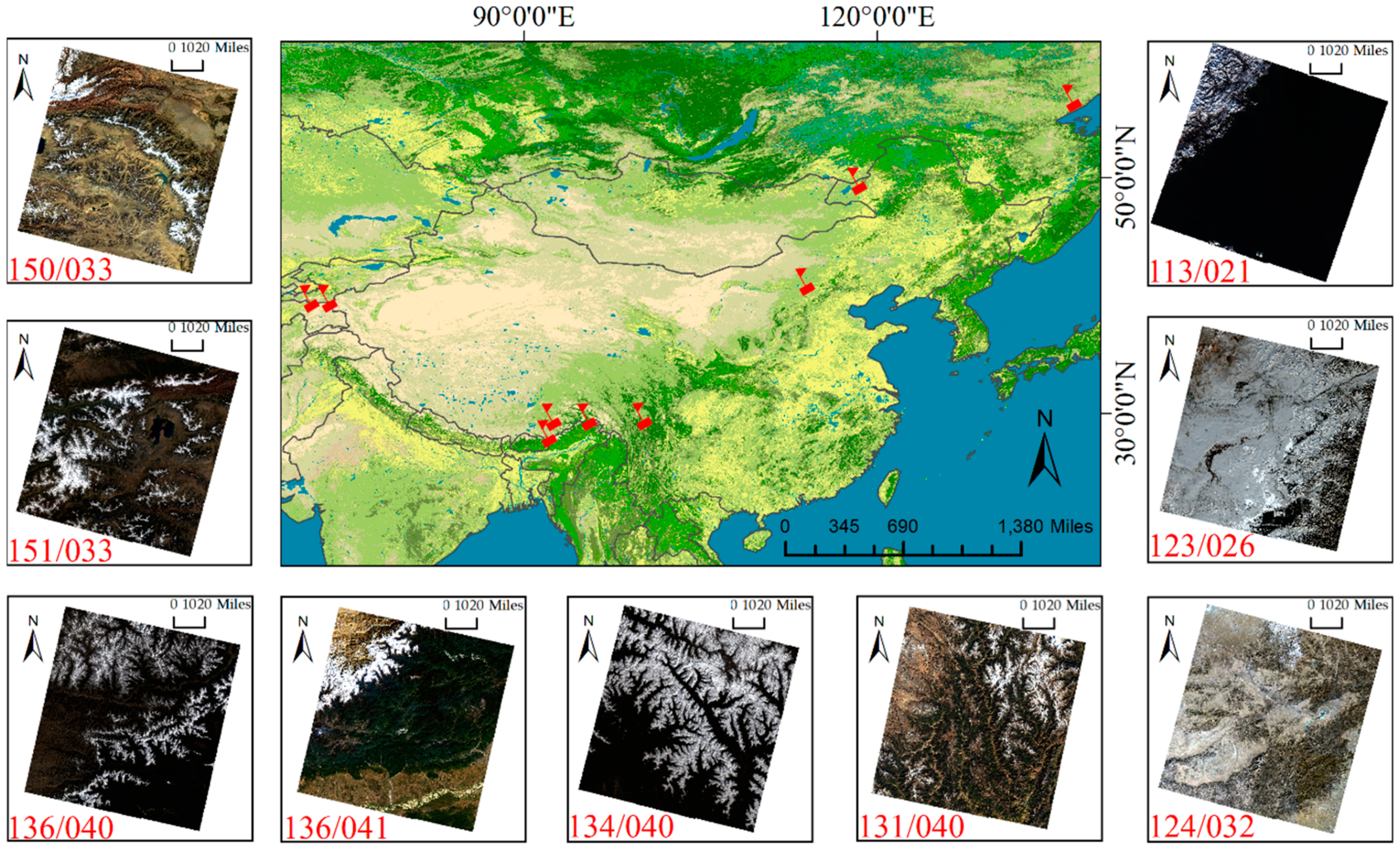
Figure 1. Sites, paths, and rows of the nine Landsat-8 Operational Land Imager (OLI) images.
Remotesensing 10 01871 g001
Figure 2. The spectral response functions of the GF-4 PMS and Landsat-8 OLI.
Remotesensing 10 01871 g002
Figure 3. Scatterplot of the GF-4 PMS reflectance versus the Landsat-8 OLI reflectance: (a) blue band; (b) green band; (c) red band; (d) NIR band. RMSE: Root Mean Square Error.
Remotesensing 10 01871 g003
Figure 4. The scatterplot of the regression values versus the real values of the reflectance of snow cover in the SWIR band.
Remotesensing 10 01871 g004
Figure 5. Histogram of the differences between the regression and real values of the reflectance of snow cover in the SWIR band.
Remotesensing 10 01871 g005
Figure 6. The structure of the multilayer feedforward neural network.
Remotesensing 10 01871 g006
Figure 7. The scatterplot of the restored reflectance versus the real reflectance of the 90,000 snow cover samples in the SWIR band.
Remotesensing 10 01871 g007
Figure 8. Histogram of the differences between the restored and real reflectance of the 90,000 snow cover samples in the SWIR band.
Remotesensing 10 01871 g008
Figure 9. Histograms of the N D S I r value of the 90,000 snow cover and 90,000 background pixels. N D S I r : The normalized difference snow index (NDSI) calculated with the restored SWIR reflectance.
Remotesensing 10 01871 g009
Figure 10. Histograms of the RSI values of the 90,000 snow cover and 90,000 background pixels.
Remotesensing 10 01871 g010
Figure 11. Flowchart of the RSI method for snow cover monitoring form GF-4 PMS imagery.
Remotesensing 10 01871 g011
Figure 12. RGB composite images of overlapping regions of two pairs of PMS and OLI images: (a) PMS image of test site No. 1; (b) OLI image of test site No. 1; (c) PMS image of test site No. 2; (d) OLI image of test site No. 2. The four subfigures have the same north arrow and scale, which are marked in the upper left corner of the figure.
Remotesensing 10 01871 g012
Figure 13. The N D S I r and RSI images calculated with the GF-4 PMS images: (a) N D S I r of test site No. 1; (b) RSI of test site No. 1; (c) N D S I r of test site No. 2; (d) RSI of test site No. 2. The four subfigures have the same north arrow and scale, which are marked in the upper left corner of the figure.
Remotesensing 10 01871 g013aRemotesensing 10 01871 g013b
Figure 14. Distribution of snow cover mapped by the RSI method from the GF-4 PMS image: (a) test site No. 1; (b) test site No. 2. The two subfigures have the same north arrow, scale, and legend, which are marked on the upper part of the figure.
Remotesensing 10 01871 g014
Figure 15. Distributions of the RSI and NDSI values of snow cover and background samples using box and whisker plots. The first and last horizontal lines of each box from top to bottom represent the maximum and minimum, respectively. The second, third, and fourth horizontal lines of each box from top to bottom represent the 25th, 50th (median), and 75th percentiles, respectively.
Remotesensing 10 01871 g015
Figure 16. Enlarged views of cloud pixels in the second test site: (a) RGB composite image of GF-4 PMS data; (b) distribution of snow cover detected by the RSI method. The two subfigures have the same north arrow and scale, which are marked in the upper left corner of the figure.
Remotesensing 10 01871 g016
Table 1. Sensor parameters of the Gaofen-4 panchromatic and multispectral sensor (GF-4 PMS) and Landsat-8 OLI.
Sensor ParametersGF-4 PMSLandsat-8 OLI
Wavelength Range/μmBlue Band0.44–0.530.45–0.51
Green Band0.51–0.610.53–0.59
Red Band0.61–0.700.64–0.67
NIR Band0.74–0.910.85–0.88
Central Wavelength/μmBlue Band0.51900.4826
Green Band0.55000.5613
Red Band0.62800.6546
NIR 1 Band0.77000.8646
Spatial Resolution/m5030
1 NIR represents the near infrared.
Table 2. The coefficients of multilinear regression per OLI image.
Path/RowInterceptCoefficient
Blue BandGreen BandRed BandNIR Band
113/210.058−0.160−0.1760.1660.213
123/260.094−0.360−0.1630.607−0.106
124/320.051−0.4580.143−0.0620.396
131/400.051−0.6370.1520.1180.390
134/400.030−0.227−0.005−0.1030.405
136/400.058−0.6870.0570.1530.507
136/410.050−0.5910.0800.1610.394
150/330.034−0.3090.044−0.3170.652
151/330.043−0.1140.153−0.4660.473
Standard deviation0.0180.2110.1260.3130.213
Table 3. The cluster centers and regression coefficients per cluster.
ClusterInterceptCoefficientCluster Center
Red BandNIR BandR&S 1N&S 2
10.004−0.1690.2530.8840.870
20.0180.1370.1020.5390.550
30.010−0.0480.1810.7400.732
1 R&S represents the normalized difference between the reflectance in the red and shortwave infrared (SWIR) bands. 2 N&S represents the normalized difference between the reflectance in NIR and SWIR bands.
Table 4. Details of the pairs of the GF-4 PMS and Landsat-8 OLI images.
Test SiteSensorAcquisition DateAcquisition TimeSolar ZenithSolar Azimuth
No. 1GF-4 PMS18 December 201610:5666.38°160.07°
Landsat-8 OLI14 December 201610:5367.12°161.90°
No. 2GF-4 PMS16 October 201611:0257.54°140.17°
Landsat-8 OLI15 October 201611:0850.01°158.35°
Table 5. Classification accuracy of the validation dataset.
CategoryProducer AccuracyUser AccuracyCommission 1Omission 2Overall Accuracy
Snow Cover95.00%99.38%0.62%5.00%97.99%
Background98.63%97.71%2.29%1.47%
1 Commission represents the fraction of samples that were predicted to be in a class, but do not belong to that class. 2 Omission represents the fraction of samples that belong to a class, but were predicted to be in a different class.
Table 6. Number of the saturation pixels in the GF-4 PMS images.
Test SiteBlue BandGreen BandRed BandNIR Band
No. 16901401027
No. 24780106810