Abstract
To obtain an accurate count of wheat spikes, which is crucial for estimating yield, this paper proposes a new algorithm that uses computer vision to achieve this goal from an image. First, a home-built semi-autonomous multi-sensor field-based phenotype platform (FPP) is used to obtain orthographic images of wheat plots at the filling stage. The data acquisition system of the FPP provides high-definition RGB images and multispectral images of the corresponding quadrats. Then, the high-definition panchromatic images are obtained by fusion of three channels of RGB. The Gram–Schmidt fusion algorithm is then used to fuse these multispectral and panchromatic images, thereby improving the color identification degree of the targets. Next, the maximum entropy segmentation method is used to do the coarse-segmentation. The threshold of this method is determined by a firefly algorithm based on chaos theory (FACT), and then a morphological filter is used to de-noise the coarse-segmentation results. Finally, morphological reconstruction theory is applied to segment the adhesive part of the de-noised image and realize the fine-segmentation of the image. The computer-generated counting results for the wheat plots, using independent regional statistical function in Matlab R2017b software, are then compared with field measurements which indicate that the proposed method provides a more accurate count of wheat spikes when compared with other traditional fusion and segmentation methods mentioned in this paper.
1. Introduction
Wheat yield is an important part of national food security [1], and spikes per unit area is an important factor in wheat yield. Obtaining a rapid and accurate count of the number of spikes per unit area is thus crucial for determining wheat yield.
With the continuous improvement in the mechanization and digitalization of agricultural production, the methods of predicting crop production have gradually diversified, and many methods are now available for small area production forecasting. These methods include field artificial prediction, capacitance measurement, climate analysis and prediction, remote sensing prediction, and prediction of the year’s harvest [2]. However, these methods have the disadvantages of being highly subjective and incurring high cost, and cannot provide accurate results for small areas. In contrast, image processing techniques provide satisfactory results for small area production forecasting.
Compared with fruit and vegetable crop counting, wheat crop counting and yield estimation based on image processing techniques are still in the relatively primitive stage. Few works have focused on counting wheat spikes, which constitutes one of the most important components of wheat yield. An automated method for predicting the yield of cereals, especially of wheat, is highly desirable because its manual evaluation is excessively time consuming. To address this issue, we propose herein to use image processing methods to count the number of wheat spikes per square meter, thereby simplifying the work of agriculture technicians.
The image processing technology based on single data source cannot guarantee spectral resolution and image resolution simultaneously because of the singleness of data sources. As a way to solve this problem, image fusion keeps the spectral characteristics of low resolution multispectral images and gives it high spatial resolution. Kong et al. proposed an infrared and visible image fusion method based on non-subsampled shearlet transform and a spiking cortical model [3]. Li et al. [4] introduced a novelty image fusion method based on a sparse feature matrix. Ma et al. [5] discussed an infrared and visible image fusion method based on a visual saliency map. Zhang et al. [6] proposed a fusion algorithm for Hyperspectral Remote Sensing Image Combined with Harmonic Analysis and Gram-Schmidt Transform which shows a good performance during the fusion operation between different resolution images. Since the Gram-Schmidt Transform has the above characteristic, it was used in our work. The key to using image processing to count wheat spikes is image segmentation [7]. In recent years, the segmentation of RGB images, or more generally multispectral images, has gained significant research attention. For example, Ghamisi et al. [8] proposed a heuristic-based segmentation technique for application to hyperspectral and color images, and Su and Hu discussed an image-quantization technique that uses a self-adaptive differential evolution algorithm, with the technique being verified by using standard test images [9]. Furthermore, Sarkar and Das [10] proposed a segmentation procedure based on Tsallis entropy and differential evolution. In image segmentation based on multi-source data, three different image features can be extracted according to different characteristics of target objects as a basis for separation of soil background: color, texture, and sharp [11]. However, at the filling stage, wheat ear and leaf have similar texture features, and cannot be identified accurately through the difference of texture [12]. Meanwhile, the severe adhesion between wheat ears is so serious that it is impossible to obtain accurate sharp information [13]. Based on these considerations, the color feature is used as the basis for image segmentation.
At present, there are many methods of image segmentation based on color features. Chen et al. [14] introduced a medical image segmentation by combining Minimum cut and Oriented Active Appearance Models. Narkhede et al. [15] used an edge detection method for color image segmentation. Gong et al. [16] proposed an efficient fuzzy clustering method in image segmentation. Pahariya et al. [17] successfully used a snake model with a noise adaptive fuzzy switching median filter method in image segmentation. Subudhi et al. [18] introduced a region growing method for Aerial Color Image Segmentation. Tang et al. [19] proposed an improved Otsu Method for Image Segmentation based gray level and gradient mapping function. Zhao et al. [20] introduced a maximum entropy method to deal with 2D image segmentation. Compared with other methods, the maximum entropy method shows robustness to the size of the interest region and is more adaptable to complex backgrounds so it could be used in the coarse segmentation operation in this paper [21].
In addition, observation methods are crucial for data acquisition, and such methods differ greatly in accuracy, stability, and duration. Establishing a rapid, accurate, high-throughput, non-invasive, and multi-phenotypic analysis capability for field crops is one of the great challenges of precision agriculture in the twenty-first century [22]. Modern agriculture demands the development of a high-throughput platform to analyze the phenotypic platforms [23]. Table 1 compares several current propositions to obtain crop phenotype (Table 1).

Table 1.
Advantages and disadvantages of current methods to obtain crop phenotype.
In view of the drawbacks with current segmentation algorithms and observation methods, we propose herein a new method to obtain wheat spike number statistics. The method exploits the field-based phenotype platform (FPP): First, high-definition digital images and the corresponding multispectral images of plots are obtained by using a home-built ground-moving phenotype platform vehicle which could overcome the limitation of bad weather conditions and high-cost. After two images are ortho corrected and registered, this paper introduces an algorithm to identify wheat ears in the filling stage. This paper also presents a novel direction to count the number of wheat ears. The analysis shown in this paper, however, can be extended for any component phenotype.
The paper has the following novel research contributions: (a) it introduces a method for optimizing threshold selection in the maximum entropy segmentation method; (b) it presents a better way for noise reduction based on morphological filters which can provides more accurate coarse-segmentation results; (c) it introduces a new direction of fine-segmentation of adhesive parts of wheat ears based on morphological reconstruction.
2. Study Site and Data Collection
2.1. Study Site
The experimental site was at the Xiaotangshan National Precision Agriculture Research and Demonstration Base, located in Changping District, Beijing, Latitude of 40°00′N–40°21′N, longitude of 116°34′E–117°00′E, altitude of 36 m. The site measured 84 m east-west, 32 m north-south, and contained 48 (6 m × 8 m) plots (Figure 1).
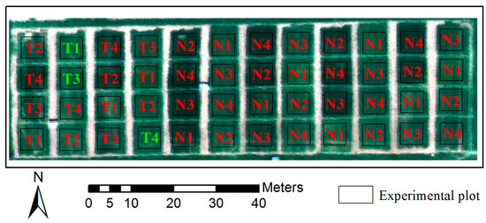
Figure 1.
Sketch map of experimental area. The image was taken on 1 May 2017 using Dajiang’s S1000 unmanned aerial vehicle. The camera model is SONY QX-100, and the UAV flying height is 50 m. The green markings represent selected areas and red markings represent other areas.
According to the planting area map, we selected three representative plots: T1 (located on the edge of the protective line), T3 (located in the middle of the wheat field), and T4 (located on the side of the wheat field). This selection minimizes the influence of the marginal effect and ensures that the quadrats are representative.
2.2. Self-Developed Semi-Autonomous Multi-Sensor Field-Based Phenotype Platform
Figure 2 shows the platform, which consists of a three-wheeled double-deck steel-frame structure. The length, width, and height of the platform are respectively 3 m, 3 m, and 3.5 m. The payload of the platform is 20 kg. The diameter of the Cloud Terrace is 0.5 m. The height control range of the sensor cantilever is 0.5 m–4 m. The speed of the platform is 1 m/s and the endurance time of the platform is 2 h. The sensor is hung from the cloud terrace, which is below the cantilever at the front end of the platform. The platform is powered by an on-board accumulator located in the middle of the platform, which supplies power to two brushless motors located at the front wheels, thereby driving the platform. The two front wheels of the platform are fixed power wheels, and the rear wheel provides steering. The minimum turning radius of the vehicle is 3 m. Both the front and rear wheels of the platform are equipped with wide rubber tires and anti-skid chains, and can handle undulating gaps of no more than 10 cm. The cloud terrace has multiple holes for hanging equipment and can simultaneously accommodate two high-definition digital cameras, a multispectral camera, a hyperspectral camera, a thermal imager, and a lidar camera for simultaneous data acquisition. The rear column of the platform contains a console to hold two laptops for data storing and real-time processing. The tail of the platform houses the operator control mechanism, which controls the speed and steering of the system. In this experiment, this platform is equipped with a multispectral camera (Parrot, Paris, France) with a resolution of 1280 × 960 and field of view of 47.2°. The spectral range of the multispectral camera is 550 nm–790 nm with a ground resolution of 1.13 mm/pix. The focal length of the multispectral camera is 35 mm. It is equipped with another high-definition digital camera (Sony DSC-QX100, Tokyo, Japan) with a ground resolution of 0.56 mm/pix and field of view of 60°.
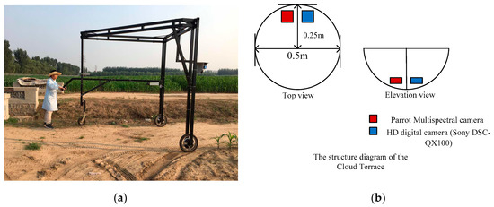
Figure 2.
Field operating diagram and photograph of field-based phenotype platform (FPP) (a) and of vehicle-mounted cloud terrace (b).
2.3. Data-Acquisition and Pre-Processing
2.3.1. Data-Acquisition
- Lighting conditions: The luminosity of the scene, especially the shadows, makes it quite difficult to visually detect wheat spikes (the same applies for our algorithms). We thus treat only well-illuminated images. The images for this work were acquired between 1 and 2 p.m. on 7 June 2017, and the intensity of the sun was about 65,000–80,000 lx at the time in order to avoid over exposure and reduce the effect of shadow.
- Growth period selection: For this study, we observed winter wheat in the filling stage because, during this period, starch produced by photosynthesis in wheat is transformed into proteins stored in the wheat seeds by assimilation. A strong correlation exists between the spike numbers and yield of mu. Obtaining an accurate count of wheat in this time period provides guidance for estimating the final yield. Moreover, during this period, the color characteristic of wheat was more prominent, which facilitates computer identification.
- Determination of observation area: A quadrat size of 50 cm × 50 cm was used in this work to match the sensor field of view of the phenotypic platform sensor. This field of view allows geometrical distortion to be effectively controlled.
- Manual statistics: While collecting data from the ground platform, we made manual statistics on the number of wheat grains in the corresponding area, and recorded the statistical results according to the number of the plots. In this way, we could synchronize the exact number of ears at the time of image shooting.
2.3.2. Data-Acquisition
1. RGB three channel fusion
In G-S fusion, we need to use multi spectral images of low spatial resolution to simulate high resolution images. Here, the high resolution image is defined as a panchromatic image. In this paper, the high resolution images we obtained are RGB images. So we use the following formula depending on the illumination characteristics to fuse the three bands of red, green, and blue, and get the corresponding high resolution panchromatic images [24].
Gray value = 0.587 × R + 0.114 × G + 0.299 × B.
2. Ortho-photo correction and image registration
By using the ortho-rectification tool from the Environment for Visualizing Images (ENVI) software, the multispectral and panchromatic images are ortho-photo corrected. The center of the corrected region is used as the projection-center point and a 50-cm-long quadrat is divided as the target region. After that, the two types of images are registered with each other. Because the two pictures have different resolutions, the panchromatic images are used as reference images and the multispectral image as the images to be registered. The images are registered by using the image registration tools in ENVI 5.3.
3. Methodology
Figure 3 shows a flow chart of the proposed method. The basic steps are the Gram–Schmidt (GS) fusion of panchromatic images and multispectral images, the determination of the maximum entropy segmentation threshold by FACT, removal of the threshold segmentation results based on morphological filters, and segmentation of the wheat adhesion region based on morphological reconstruction (MR). First, the GS algorithm is used to improve information quality of the image, following which FACT is used to determine the segmentation threshold, and then the maximum entropy method segmentation method is applied for threshold segmentation. Next, the segmentation results are de-noised based on the clustering method and, finally, the adhesive parts of the target are treated by MR. These components are described in detail in the following subsections (Figure 3).
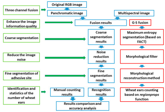
Figure 3.
Flow chart of recognition and counting method of wheat ear at filling stage.
3.1. Fusion of Panchromatic Images and Multispectral Images Based on Gram-Schmidt Spectral Sharpening
The spatial resolution of multispectral images is improved by the fusion of high spatial resolution panchromatic images and corresponding low resolution multispectral images. Here, the Gram-Schmidt spectral sharpening method is used to achieve this goal.
- Using the gray value Bi of the i band of the multispectral image, the gray value of the whole color band P is simulated according to the weight of the Wi, that is:
- The panchromatic image is used as the first component for the GS transform of the simulated multispectral image;
- The statistical value of the panchromatic image is adjusted to match the first component G-S1 after the G-S transform to produce a modified image;
- A new data set is generated by replacing the first component of the G-S transform with a modified high resolution band image;
- A multispectral image enhanced by spatial resolution can be obtained by inverse G-S transform to the new data set.
3.2. Maximum Entropy Threshold Segmentation for Threshold Selection of Firefly Algorithm Based on Chaos Theory
The traditional maximum entropy method is not sensitive to target size and can only be used for image segmentation of small targets. In addition, it provides better segmentation results for images of different target sizes and signal-to-noise ratios. The maximum-entropy method segments the image by maximizing the entropy of the segmented image. Therefore, the choice of the optimal threshold plays a decisive role in the segmentation effect. The global ergodic method, which is a conventional threshold-determination method, traverses all the gray levels to find the optimal threshold. However, this method is time consuming and computationally complex, especially for complex image multi-threshold segmentation, making it unsuitable for real-time processing.
To solve these problems, we improve the standard Firefly Algorithm (FA) and propose a new method called FACT. Here, the firefly represents the pixel of the image. For FACT, the movement of fireflies is very important because it determines the optimization ability of the algorithm. The movement of a common firefly is manifested as follows:
When fireflies Xi and Xj attract each other, Xi moves toward Xj if I(xj) >I(xi) and its new location is determined by
where t stands for evolutionary algebra, β indicates the degree of attraction, α∈[0,1] represents the step length factor, and r1 is a random number whose distribution is uniform over [0,1]. When r1 < 0.5 (r1 > 0.5), Xm is set to UB − Xi (T) [Xi(T) − LB], where UB and LB denote the upper and lower bounds of the defined domain, respectively.
Equation (1) consists of three terms: The first term, Xi(T), indicates the current position of the firefly. The second term, β[Xj(T) − Xi(T)], represents the change in Xi caused by the attraction between Xj and Xm; this leads to global optimization. The third term, α(r1 − 0.5)Xm, is the local random fluctuation and provides local optimization.
Because the brightest firefly XB cannot be attracted by other fireflies, its motion cannot be described by Equation (1), so we propose the following:
where t represents evolutionary algebra and r2 is a random number uniformly distributed over [0,1]. If r2 < 0.5 (r2 > 0.5), Xm is set to UB − Xi (T) [Xi(T) − LB].
We see from the discussion of the firefly motion (Equation (1)) that the local search term is only a random search. Therefore, the local mining capacity of the algorithm is weak. To overcome this shortcoming, we use a local search operator based on chaotic sequences.
The basic idea of the new operator is to use the randomness, ergodicity, and regularity of chaotic sequences to perform a local search. This operator consists of five specific steps:
- (a)
- In the firefly population, {Xi; i = 1, …, NP}, a firefly vector XB is selected at random from the first p individuals with the best quality. The threshold of p is chosen to be 5%.
- (b)
- The chaotic variable chi is generated by using logistic chaotic formulawhere , chi ≠ 0.25, 0.5, 0.75, and chi is a random number evenly distributed over the range (0, 1). The length of the chaotic sequence is expressed by K.
- (c)
- The following equation is used to map the chaotic variable chi into the chaotic vector CHi defined over the domain (LB, UB)
- (d)
- The chaotic vector CHi and XB are linearly combined to generate candidate firefly vectors Xc by usingwhere represents the contraction factor and is defined bywhere maxIter represents the maximum number of iterations of the algorithm, and t indicates the current iteration number.
- (e)
- We now select between the candidate firefly vector Xc and the current optimal firefly vector Xb. If Xc replaces Xb or the length of the chaotic sequence reaches K, the local search ends. If neither of these criteria is met, we go to step (b) and begin a new iteration.
The pseudocode of the chaotic FA based on the basic FA is as follows:
| Pseudocode for chaotic firefly algorithm |
| (i) Random initialization of firefly populations{Xi(0)|i = 1,…NP} |
| (ii) Calculate brightness I according to the target function f |
| (iii) for t = 1:maxIter |
| (iv) for i = 1:n |
| (v) for j = 1:n |
| (vi) if [I(Xj(t)] > I(Xi(t) |
| (vii) Move to the firefly Xi(t) according to (iv) |
| (viii) end if |
| (ix) end for j |
| (x) end for i |
| (xi) Local search using chaotic local operators |
| (xii) Move to the best firefly Xb(T) according to (v) |
| (xiii) end while |
3.3. De-Noise Operation Based on Morphological Filters
After coarse segmentation is complete, a large number of unclassified noise points still exist in the coarse segmentation results which will affect the accuracy of computer identification. To remove these points without affecting the segmentation results, we use a de-noising method based on morphological filters. Compared with other de-noising methods like the spherical coordinates system [25], the noise standard deviation (SD) estimation method [26], and the multi-wavelet transform method [27], the morphological filters have a better performance in dealing with details [28]. We now introduce the principle of this method.
Let f be the result of threshold segmentation. CB (morphology based on contour structure elements) morphological dilation DB(f) and erosion-operation results EB(f) with f based on structural element B are given as
where B stands for a structural element, is the dilation operation operator, and is the erosion operator.
CB morphological open and closed operations and operators CBOB(f) and CBCB(f) with f based on structural element B is expressed as
Compared with the classical morphological open and closed operators, the CB morphological open and closed operations defined by Equations (9) and (10) have more filtering power. These algorithms, however, filter out more details. Therefore, in this work, we propose the following filter definitions:
where Bi and Bj indicate different or identical structural elements.
The algorithm proceeds as follows:
- (a)
- After the original images are segmented by the threshold, two parts are obtained, called foreground target O and background target B. The target O is filtered with the filters FOij(f) and FCij(f), and the results are labeled O1 and O2, respectively. The background B is filtered with the filters NOij(f) and NCij(f), and the results are labeled B1 and B2, respectively. Next, the weighted mergings of O1 and O2 and B1 and B2 are called the merged foreground and background and , respectively:where , , , and are weights. The coefficients of and control the brightness of the target and background (detail clarity), and the coefficients of and control the dim degree of the two objects above (smoothness).
- (b)
- Repeat step (a) for each new foreground target O and background B. The number of repeated operations is N.
- (c)
- Reform the N iteration results with foreground targets and background to obtain the new image .
- (d)
- Repeat steps (a)–(c) for , with the number of repeating operation being M. This gives the filtered image .
Given that the time complexity of the algorithm increases with the growth of M, we need to select M appropriately to make the filtering details more prominent. The larger N is, the more blurred is the image . However, if the value of N is too small, the filter’s ability to filter out noise weakens. Therefore, the value of N for the image with serious noise pollution can be increased. Usually, M takes on a value from the set {1, 2, 3, 4} and N from the set {1, 2, 3}. Here, to obtain an intuitive feel for the effect of de-noising, we use an area of size 50 cm × 50 cm for the filtering experiments (Figure 4).
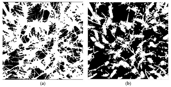
Figure 4.
Image contrast before and after morphological filtering. (a) Before morphological filtering, (b) after morphological filtering.
Figure 4 shows that, after the original image is filtered by the proposed morphology filter, the number of noise points in the selected region is reduced, and the curve of objects is more prominent.
3.4. Fine-Segmentation of the Wheat Adhesion Region Based on Morphological Reconstruction
After the threshold segmentation and de-noising process, the objects in the foreground region remain stuck to each other and need to be further segmented. Each object has two boundaries: one is the boundary between the foreground object and the background area, and the other is the boundary between the objects that are stuck together. These are all located in the foreground area where the threshold was segmented, and the segmentation results can be achieved by determining these boundaries. In the foreground region where the threshold is segmented, the gray value of the boundary region adjacent to the background region is greater than the gray value of the region surrounding it [29]. Therefore, the boundaries of all the objects to be segmented in the pretreated graph have locally higher gray values. The dome can be defined as a region with a larger gray value in the local region, and the above boundary region is considered as a dome [30], so it can be extracted by grayscale morphological reconstruction. To avoid missing boundary points, different domes are extracted in different directions. In this work, we select six directions in equal intervals from 0° to 180°.
3.5. Wheat Ear Detection and Statistics
After the above operation, we get several separate and disconnected bright areas, each of which represents an unidentified wheat ear. Here, we use the regionprops function in Matlab R2017b to count the independent regions in the image so as to count the number of wheat ears. Meanwhile, we processed Ground Truth operation for each image, and manually labeled the wheat ears in the image, so as to compare with the result of computer recognition.
4. Results
4.1. Multispectral and Panchromatic Image Fusion Results Based on the Gram–Schmidt Algorithm
After pre-processing with ortho-photo correction and image registration, the two types of images are fused by using the GS transform. Figure 5 shows the original panchromatic images and the corresponding fusion results, respectively (Figure 5).
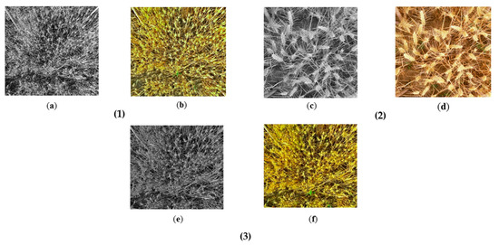
Figure 5.
Fusion results of original panchromatic and multispectral images after registration. (1) Image contrast before and after fusion in T1 plot: (a) Panchromatic image with T1 plot; (b) Fusion result in T1 plot; (2) Image contrast before and after fusion in T3 plot: (c) Panchromatic image with T3 plot; (d) Fusion result in T3 plot; (3) Image contrast before and after fusion in T4 plot: (e) Panchromatic image with T4 plot; (f) Fusion result in T4 plot.
Based on the visual effects, we conclude that the edges of the images are clearer after fusing, and that the contrast ratio between foreground and background is greater. After completing the manual evaluation, we then judge the original RGB images and fusion results by several image indicators. As shown in Table 2, six indicators for evaluation have been selected to evaluate the display effect of the images before and after the fusion with different fusion methods, including mean value (MV), SD, information entropy (IF), mean gradient (MG), spatial frequency (SF), and edge intensity (EI) [31,32,33] (Table 2). The greater the value of the above six indicators, the better the image display effect is.
Table 2.
Results of image display effect evaluation before and after fusion with different fusion methods. Mean Value (MV); Standard Deviation (SD); Information Entropy (IF); Mean Gradient (MG); Spatial Frequency (SF); Edge Intensity (EI).
From the contrast results of Table 2, we can draw the conclusion that the G-S transform could get better fusion results in the display effect which could provide more abundant and clear details for the subsequent recognition processing.
In addition, we introduced other four indexes to evaluate the effect of fusion, including correlation coefficient (CC), erreur relative globale adimensionnelle de synthese (ERGAS), root mean square error (RMSE), and bias [34,35,36]. The physical meaning of the above evaluation indexes are: The ideal value of bias and RMSE are 0 and the smaller the value, the more the fusion results can maintain spectral information. The ideal value of CC is 1. The value of ERGAS is greater than 3, which shows the poor quality of the fused image while less than 3 shows that the quality of the fused image is good (Table 3).
Table 3.
Results of image fusion effect evaluation with different fusion methods. Correlation coefficient (CC); Erreur relative globale adimensionnelle de synthese (ERGAS); Root mean square error (RMSE).
From Table 3, we can see that compared with the image fusion in some other applications, the value of the fusion indexes obtained in this paper show a poor fusion effect, especially in CC and ERGAS [37,38,39]. Since all the methods were common used, this situation may be caused by the original image data. In data acquisition at the near ground level, the disturbance of the instrument itself and the influence of the shadow could reduce the quality of the acquired image. The lower quality of the original image might affect the final fusion results [40]. In the evaluation of multiple indicators, each fusion method had its own advantages and disadvantages. Among them, the CC shows the degree of change of the image before and after the fusion which is crucial to the accuracy of subsequent treatment [41]. In order to preserve the characteristics of the original image to the maximum extent, we choose the G-S transform with the highest CC as the fusion method of this paper.
However, it is impossible to judge whether the use of image fusion could have a positive impact on the accuracy of recognition from these indexes. Meanwhile, the above indexes could not estimate the effect of different fusion methods on the recognition accuracy. In the following, we further analyze the effect of image fusion on the accuracy of recognition and the effect of different fusion methods on the recognition accuracy.
4.2. Image-Segmentation Results
With the multispectral and panchromatic fusion images obtained above, we first use the method proposed herein to segment the images and determine the number of wheat spikes. Following this, several traditional methods are used to do the contrast tests (Figure 6). Because the number of wheat spikes in the observation region T3 is small, we mark the results of ground truth and machine identification results, so as to show the accuracy of this method more intuitively.
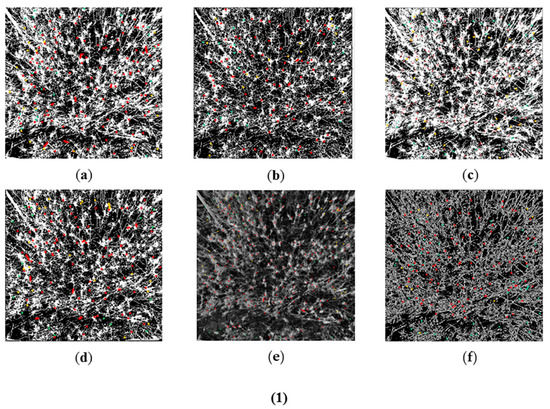
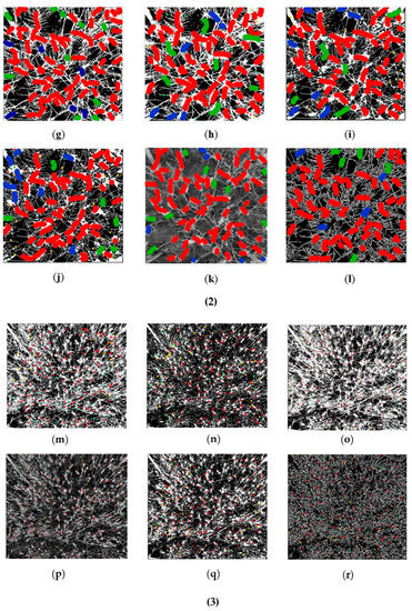
Figure 6.
Segmentation results in each plot. Red regions show where artificial and machine recognition agree, blue regions show where artificial recognition and machine recognition do not agree, green regions show where the machine gives erroneous recognition. (1) Segmentation results in T1 plot: (a) Proposed method; (b) Edge detection method; (c) fuzzy clustering method; (d) Snake model; (e) Minimum cut method; (f) region growth method; (2) Segmentation results in T2 plot: (g) Proposed method; (h) Edge detection method; (i) fuzzy clustering method; (j) Snake model; (k) Minimum cut method; (l) region growth method; (3) Segmentation results in T3 plot: (m) Proposed method; (n) Edge detection method; (o) fuzzy clustering method; (p) Snake model; (q) Minimum cut method; (r) region growth method.
The number of wheat grains obtained after the segmentation of different methods is calculated statistically and compared with the values obtained from artificial measurement of the plots (Table 4, Figure 7).
Table 4.
Wheat ear recognition results with different coarse segmentation methods and manual counting results.
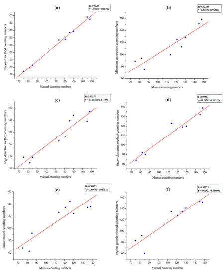
Figure 7.
Image segmentation results compared with results of manual measurements.
From Table 4 and Figure 7, we can see that after comparing with other coarse-segmentation methods, the R2 between the proposed segmentation results and manual counting results is closer to 1 which means this method could provide a statistic value much closer to the real value and has a higher accuracy. However, the R2 is not a very precise measure of the index, so we will provide more appropriate indicators to confirm this conclusion below. (a) R2 between proposed method and manual counting; (b) R2 between Minimum cut method and manual counting; (c) R2 between Edge detection method and manual counting; (d) R2 between fuzzy clustering method and manual counting; (e) R2 between snake model method and manual counting; (f) R2 between region growth method and manual counting.
5. Discussion
5.1. Analysis of Effect of Coarse-Segmentation Method on Recognition Accuracy
Image segmentation is a fundamental technique in image processing [42] and is the premise of object recognition and image interpretation. An image-segmentation problem typically involves extracting the consistent region and objects of interest from an image-processing process [43].
Based on the results presented in Table 4 and Figure 7, we conclude that the segmentation results obtained by the algorithm proposed herein are closer to the actual measured values in different regions and for different vegetation coverage conditions, which means that this method has the advantages of high accuracy and good robustness in different areas.
After comparing numerical accuracy, the segmentation results are quantitatively analyzed by using successive inter-regional contrast (Table 5), intra-regional uniform measure (Table 6), and segmentation accuracy (Table 7) [44,45]. The inter-region contrast index is a measurement of image segmentation quality based on inter-regional contrast where the smaller value represents the better segmentation effect. The uniform measurement value judges the internal uniformity of the segmentation results and a bigger value means a better effect. After that, the segmentation results obtained by computer recognition were compared with the results of artificial ground truth to get the segmentation accuracy (Table 5, Table 6 and Table 7).
Table 5.
Inter-region contrast values for different segmentation methods.
Table 6.
Uniform measurement values of regions for different segmentation methods.
Table 7.
Segmentation accuracy of different segmentation methods.
From all of the above tables, we can draw the conclusion that compared with the other segmentation methods, the method proposed in this paper could achieve more accurate image segmentation. Moreover, it can effectively control the occurrence of over segmentation and under segmentation.
5.2. Analysis of Effect of Fusion Method on Recognition Accuracy
Several different fusion methods have been used before to fuse the two different resolution images. After that, several indexes were introduced to evaluate the fusion process and fusion results. However, it is not clear whether image fusion has a positive impact on recognition accuracy. Meanwhile, the effect of different image fusion methods on recognition accuracy has not been discussed. Here, the accuracy of wheat ear recognition is compared in the following five cases: Without image fusion, image fusion based on the G-S method, image fusion based on non-sub sampled shearlet transform, image fusion based on the sparse feature matrix, and image fusion based on the visual saliency map.
From Figure 8, we obtain the following conclusions that compared with other fusion algorithms, the G-S method has the most obvious improvement in final recognition accuracy. Meanwhile, in the repeated experiments of three plots, the recognition accuracy obtained by image fusion was improved by 3–12% compared to the result without image fusion which shows that image fusion operation had a positive impact on recognition accuracy.
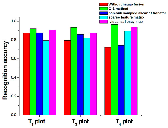
Figure 8.
Accuracy of wheat ear recognition with different image fusion methods and without image fusion.
5.3. Analysis of the Effect of Illumination Intensity on Recognition Accuracy
In previous contrast experiments, the images used were captured under the same illumination conditions. The experimental results indicate that, when the light intensity is stable at 30,000–50,000 lx, after the image is transformed into a two-valued image, the gray values of the foreground and background objects vary greatly [46]. These satisfactory results can be obtained by means of computer segmentation and recognition. However, in actual field applications, it is impossible to ensure that the intensity of illumination remains within this range [47]. To further analyze the effect of illumination intensity on the segmentation algorithm, we designed the following experiment: The control variables for this experiment are listed in Table 8.
Table 8.
Control variables for experiment on effect of illumination intensity.
In clear weather, data were collected at different times of a given day for each plot of crops. The acquisition times were at 8 a.m., 12 a.m., and 4 p.m. At the same time, the shutter was used to control the light input into the sensor by partially blocking the incident light outside the field of view of the sensor, and the illumination intensity at the center of the lens was measured precisely by the luminometer. In this experiment, two sensors were placed at a height of 1.5 m above the ground. The illumination intensity was maintained within the range of 5000–80,000 lx. A total of 11 gradients were selected, and the change in illumination intensity between the adjacent gradient was 7500 lx (Figure 9).
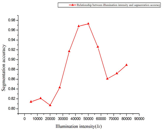
Figure 9.
Segmentation accuracy as a function of illumination intensity.
Figure 9 shows that, when the illumination intensity is within the range of 35,000–55,000 lx, the precision of the segmentation method is satisfactory. In the interval 5000–35,000 lx and 35,000–80,000 lx, the segmentation precision decreases significantly, which indicates that the proposed method is very sensitive to illumination intensity [48].
The fluctuation of segmentation accuracy caused by light intensity is mainly caused by the projection and reflection from the wheat. These two factors may lead to changes in the distribution of R, G, and B components in the captured panchromatic image. Figure 9 shows that, when the illumination intensity is less than 35,000 lx, the segmentation precision fluctuates less. This shows that wheat leaves do not cast shadows or reflect light under low-light conditions. However, because of the low reflectivity, the background soil and foreground crops cannot be accurately judged from the acquired images. When the illumination intensity is 35,000–50,000 lx, the segmentation accuracy is improved due to the improvement of illumination conditions. When the light intensity is greater than 50,000 lx, the shadow of the projection of the wheat itself is very obvious, and the reflection of the target itself begins to appear, which leads to a change in the distribution of the RGB components in the resulting panchromatic image, resulting in an increase in segmentation error.
5.4. Analysis of Sample Size
For this work, three experimental plots with three randomly selected quadrats were used for repeated tests. The data redundancy basically meets the requirement. However, because of the particularity of field experiments, these data cannot fully represent the segmentation results of all areas of the field. Moreover, the growth stage of the wheat varies from place to place and the phenotypic type differs significantly between plots. The comparative experiments on different growth stages represent a deficiency of the experimental design.
5.5. Analysis of Observation Range on Recognition Accuracy
To determine the area in which the algorithm is applicable, we extend the shooting range by increasing the height of the cantilever. After determining the central projection point, we take the point as the center and divide the research area into circles of different radii. The radius of the study area ranges from 0.25 to 0.75 m. The proposed method is used to process the image from this region, and the results are compared with the results of manual statistics. Similarly, the red dots indicate part of the artificial and machine recognition agreement, purple points represent points of artificial recognition and where machine identification is not possible. The orange dots indicate where machine identification is erroneous (Figure 10).
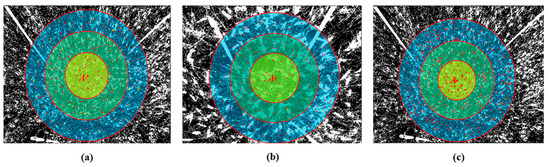
Figure 10.
Segmentation accuracy within different radii upon using proposed method. The yellow, green, and blue areas indicate an observation radius of 0–0.25 m, 0.25–0.5 m, and 0.5–0.75 m. The point A is the ortho center of the image. (a) Observation range analysis in T1 plot; (b) Observation range analysis in T3 plot; (c) Observation range analysis in T4 plot.
Figure 10 shows that, when the observation radius reaches 0.5 m, using the proposed method of segmentation and recognition can achieve results with good statistics. Extending the radius to 0.5–0.75 m results in a rapid decrease in the accuracy of the algorithm (Figure 11).
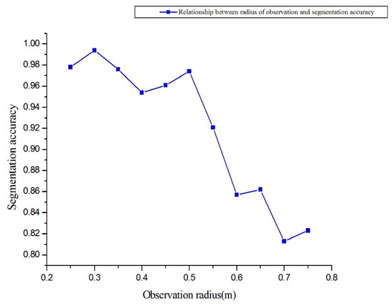
Figure 11.
Segmentation accuracy as a function of observation radius.
In view of these experimental results, we make the following analysis:
1. Influence of sensor resolution and pattern noise
For a small observation area, the camera is close to the target. In contrast, when viewing a large area, the camera is higher above the target, thereby reducing the sharpness of the target. When the observation radius reaches 0.5–0.75 m, the edge details of the target begin to blur in the image due to the resolution limit of the camera. This effect hinders the segmentation of adhesions [49]. In addition, because of the increased observation area, the amount of noise and information in the image both increase [50]. When the noise exceeds the tolerance of the filter, the residual noise point begins to affect the statistical results [51]. Moreover, the change in image resolution with the new acquisition system may also impact the parameter values. At present, we have not obtained images of the same plot with the two different digital cameras, so we cannot deduce which effect is dominant [52].
2. Influence of image-edge distortion
Due to the plateau height of the ground phenotype constraints, sensors can only capture images of a certain area [53]. The nearer the wheat spike is to the edge of the image, the more obvious is the morphological aberration [54]. In addition, the excessive deformation affects computer-vision target recognition. Two main types of edge distortion exist: barrel and pincushion distortion.
Here, we use Matlab R2017b to correct barrel and pincushion distortion, following which we segment the corrected image in succession (Figure 12).
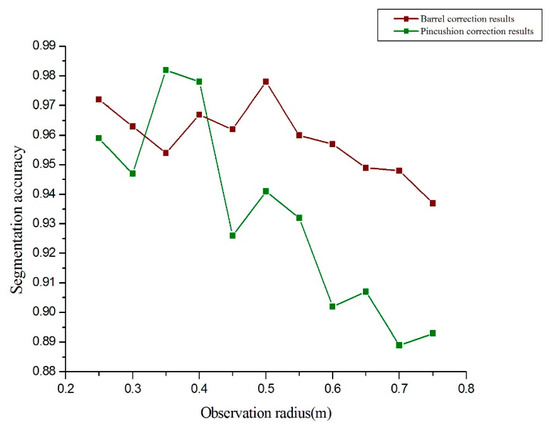
Figure 12.
Segmentation accuracy as a function of observation radius after two types of distortion.
Figure 12 shows that barrel correction significantly improves the image segmentation accuracy when the observation radius continues to expand [55]. For small observation radius, pincushion correction leads to slight improvement of the image segmentation accuracy [56], but a significant improvement in accuracy occurs for a larger observation radius. We thus conclude that the main factor leading to the decrease in accuracy is the edge barrel distortion when the segmentation area increases [57].
5.6. Accuracy Analysis of Manual Statistics
The proposed method gives satisfactory results for images taken at the mature period because the ears do not have a lot of overlaps [58]. However, because our objective is not to determine the exact shape but only the right location of each spike, these locations can be represented by a few pixels, which may sometimes be accidentally erased when cleaning the images. Thus, errors in the counting results may also be due to such imperfections. A study at the pixel level is needed to solve this dilemma. Concerning the counting level, improvements should be possible through the threshold segmentation of a new type of firefly. However, above all, the present results should be compared with manual counting, which can only be done just before the harvest.
5.7. Analysis of the Algorithm Efficiency
Speed is also critical for image segmentation applications [59]. In this paper, average running time is used to evaluate the algorithm efficiency [60]. The average running-times of several methods are shown in Figure 13. Here, we use the G-S method to complete the image fusion (Figure 13).
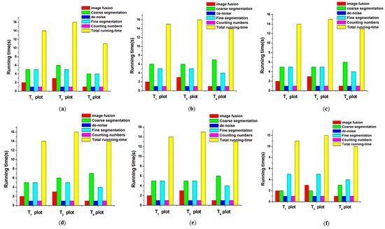
Figure 13.
Comparison of running-times by using different coarse-segmentation methods. (a) Coarse-segmentation with Minimum cut; (b) Coarse-segmentation with Edge detection; (c) Coarse-segmentation with fuzzy clustering; (d) Coarse-segmentation with snake model; (e) Coarse-segmentation with region growth; (f) Coarse-segmentation with proposed method.
From Figure 13, we can see that the average running times of different coarse segmentation methods are respectively: 13.6 s, 15 s, 14 s, 14.7 s, 14 s, and 11 s. The method proposed in this paper has the shortest running-time. As the other steps are the same, the improvement of the coarse segmentation efficiency is the key to the shortening of the time. The use of the global search ability of the firefly, which greatly reduces the search time of the optimal, leads us to conclude that the algorithm is less computationally complex and improves the speed of image coarse segmentation, making it better suited for real-time image segmentation.
6. Conclusions
We propose herein a new algorithm based on a land phenotype platform for counting wheat spikes. First, the images are acquired by a home-built ground phenotype platform. The panchromatic and multispectral images are fused by using the G-S fusion algorithm, which improves the detail of information. Next, the target function is obtained by using the maximum-entropy method, the optimal threshold of the image is found by using the FACT, and the image is segmented with this threshold. The experimental results show that the proposed method improves the segmentation accuracy and segmentation speed, has good noise immunity, and is highly robust. By solving some shortcomings of the conventional methods, such as long segmentation time and excessive computational complexity, it opens a broad range of applications in the field of precision agriculture yield estimation.
Experimental results show that the improved algorithm is competitive compared with the existing method. However, these results also show that the chaotic local search operator can significantly improve the performance of the initial evolution algorithm, whereas the latter is limited. To further improve the performance of the algorithm, the next step is to combine other local search techniques with chaotic local search operators.
Acknowledgments
This work was supported by the National Key Research and Development Program of China (2016YFD0300602), the National Key Research and Development Program of China (grant number 2016YFD0800904), the Natural Science Foundation of China (61661136003, 41471285, and 41471351), and the Special Funds for Technology innovation capacity building sponsored by the Beijing Academy of Agriculture and Forestry Sciences (KJCX20170423, KYCXPT201703). Beijing Municipal Science and Technology Project (Z161100004516009). We are grateful to the anonymous reviewers for their valuable comments and recommendations.
Author Contributions
Chengquan Zhou and Guijun Yang conducted the data analysis and drafted the article; Dong Liang designed the experimental process; Bo Xu, Xiaodong Yang, provided the data and figures about the field-based phenotyping; All authors gave final approval for publication.
Conflicts of Interest
The authors declare that the research was conducted in the absence of any commercial or financial relationships that could be construed as a potential conflict of interest.
References
- Ayas, S.; Dogan, H.; Gedikli, E.; Ekinci, M. Microscopic image segmentation based on firefly algorithm for detection of tuberculosis bacteria. In Proceedings of the Signal Processing and Communications Applications Conference (SIU), Malatya, Turkey, 16–19 May 2015; pp. 851–854. [Google Scholar] [CrossRef]
- Azzari, G.; Lobell, D.B. Satellite estimates of crop area and maize yield in Zambia’s agricultural districts (Abstracts). In Proceedings of the AGU Fall Meeting, San Francisco, CA, USA, 14–18 December 2015. [Google Scholar]
- Kong, W.; Wang, B.; Lei, Y. Technique for infrared and visible image fusion based on non-subsampled shearlet transform and spiking cortical model. Infrared Phys. Technol. 2015, 71, 87–98. [Google Scholar] [CrossRef]
- Li, H.; Li, L.; Zhang, J. Multi-focus image fusion based on sparse feature matrix decomposition and morphological filtering. Opt. Commun. 2015, 342, 1–11. [Google Scholar] [CrossRef]
- Ma, J.; Zhou, Z.; Wang, B.; Zong, H. Infrared and visible image fusion based on visual saliency map and weighted least square optimization. Infrared Phys. Technol. 2017, 82, 8–17. [Google Scholar] [CrossRef]
- Zhang, T.; Liu, J.; Yang, K.M.; Luo, W.S.; Zhang, Y.Y. Fusion Algorithm for hyperspectral remote sensing image combined with harmonic analysis and gram-schmidt transform. Acta Geod. Cartogr. Sin. 2016, 44, 1042–1047. [Google Scholar] [CrossRef]
- Pal, N.R.; Pal, S.K. A review on image segmentation techniques. Pattern Recognit. 1993, 26, 1277–1294. [Google Scholar] [CrossRef]
- Ghamisi, P.; Couceiro, M.S.; Martins, F.M.L.; Benediktsson, J.A. Multilevel image segmentation based on fractional-order Darwinian particle swarm optimization. IEEE Trans. Geosci. Remote Sens. 2014, 52, 2382–2394. [Google Scholar] [CrossRef]
- Su, Q.; Hu, Z. Color image quantization algorithm based on self-adaptive differential evolution. Comput. Intell. Neurosci. 2013. [Google Scholar] [CrossRef] [PubMed]
- Sarkar, S.; Das, S. Multilevel image thresholding based on 2D histogram and maximum Tsallis entropy—A differential evolution approach. IEEE Trans. Image Process. 2013, 22, 4788–4797. [Google Scholar] [CrossRef] [PubMed]
- Mukherjee, D.; Wu, Q.M.J.; Wang, G. A comparative experimental study of image feature detectors and descriptors. Mach. Vis. Appl. 2015, 26, 443–466. [Google Scholar] [CrossRef]
- Zhy, C.; Gu, G.; Liu, H.; Shen, J.; Yu, H. Segmentation of ultrasound image based on texture feature and graph cut. In Proceedings of the 2008 International Conference on Computer Science and Software Engineering, Wuhan, China, 12–14 December 2008; pp. 795–798. [Google Scholar]
- Tan, W.; Yan, B.; Li, K.; Tian, Q. Image retargeting for preserving robust local feature: Application to mobile visual search. IEEE Trans. Multimed. 2015, 18, 128–137. [Google Scholar] [CrossRef]
- Chen, X.; Udupa, J.K.; Bagci, U.; Zhuge, Y.; Yao, J. Medical image segmentation by combining graph cuts and oriented active appearance models. IEEE Trans. Image Process. 2012, 21, 2035–2046. [Google Scholar] [CrossRef] [PubMed]
- Narkhede, P.R.; Gokhale, A.V. Color image segmentation using edge detection and seeded region growing approach for CIELab and HSV color spaces. In Proceedings of the International Conference on Industrial Instrumentation and Control, Pune, India, 28–30 May 2015. [Google Scholar] [CrossRef]
- Gong, M.; Su, L.; Jia, M.; Chen, W. Fuzzy clustering with a modified MRF energy function for change detection in synthetic aperture radar images. IEEE Trans. Fuzzy Syst. 2014, 22, 98–109. [Google Scholar] [CrossRef]
- Pahariya, S.; Tiwari, S. Image segmentation using snake model with nosie adaptive fuzzy switching median filter and MSRM method. In Proceedings of the 2015 IEEE International Conference on Computational Intelligence and Computing Research (ICCIC), Madurai, India, 10–12 December 2015. [Google Scholar] [CrossRef]
- Subudhi, B.N.; Nanda, P.K.; Ghosh, A. Entropy based region selection for moving object detection. Pattern Recognit. Lett. 2011, 32, 2097–2108. [Google Scholar] [CrossRef]
- Tang, Y.S.; Xia, D.H.; Zhang, G.Y.; Ge, L.N.; Yan, X.Y. The detection method of lane line based on the improved Otsu threshold segmentation. Appl. Mech. Mater. 2015, 741, 354–358. [Google Scholar] [CrossRef]
- Zhao, W.; Ye, Z.; Wang, M.; Ma, L.; Liu, W. An image threholding approach based on cuckoo search algorithm and 2D maximum entropy. In Proceedings of the 2015 IEEE 8th International Conference on Intelligent Data Acquisition and Advanced Computing Systems: Technology and Applications (IDAACS), Warsaw, Poland, 24–26 September 2015. [Google Scholar] [CrossRef]
- Wang, Y.; Dai, Y.; Xue, J.; Liu, B.; Ma, C.; Gao, Y. Research of segmentation method on color image of Lingwu long jujubes based on the maximum entropy. EURASIP J. Image Video Process. 2017, 1. [Google Scholar] [CrossRef]
- Rokhmana, C.A. The potential of UAV-based remote sensing for supporting precision agriculture in Indonesia. Procedia Environ. Sci. 2015, 24, 245–253. [Google Scholar] [CrossRef]
- Liang, H.C.; Lu, H. Minimum cuts and shortest cycles in directed planar graphs via noncrossing shortest paths. SIAM J. Discret. Math. 2017, 31, 454–476. [Google Scholar] [CrossRef]
- Sang, N.T.; Van, T.M.N.; Van, A.H.; Lung, V.D. A novel method for video enhancement-RGB local context-based fusion. In Proceedings of the 2015 International Conference on Image and Vision Computing New Zealand (IVCNZ), Auckland, New Zealand, 23–24 November 2015. [Google Scholar] [CrossRef]
- Zhang, D.; Kang, X.; Wang, J. A novel image de-noising method based on spherical coordinates system. EURASIP J. Adv. Signal Process. 2012, 2012. [Google Scholar] [CrossRef]
- Suzuki, T.; Tsuji, H.; Taguchi, A.; Kimura, T. A Estimate method of standard deviation for Gaussian noise with image information. In Institute of Electronics, Information and Communication Engineers (IEICE) Technical Report; Intelligent Multimedia System, General; Institute of Electronics, Information and Communication Engineers: Tsuruoka, Japan, 2014. [Google Scholar]
- Gao, L.; Wang, G.; Liu, J. Image denoising based on edge detection and prethresholding wiener filtering of multi-wavelets fusion. Int. J. Wavelets Multiresolut. Inf. Process. 2015, 13. [Google Scholar] [CrossRef]
- El Hassani, A.; Majda, A. Efficient image denoising method based on mathematical morphology reconstruction and the Non-Local Means filter for the MRI of the head. In Proceedings of the 4th IEEE International Colloquium on Information Science and Technology (CiSt), Tangier, Morocco, 24–26 October 2016. [Google Scholar] [CrossRef]
- Wu, Y.; Peng, X.; Ruan, K.; Hu, Z. Improved image segmentation method based on morphological reconstruction. Multimed. Tools Appl. 2016, 76, 19781–19793. [Google Scholar] [CrossRef]
- Wu, J.; Cao, F.; Yin, J. Nonlocally multi-morphological representation for image reconstruction from compressive measurements. IEEE Trans. Image Process. 2017, 26, 5730–5742. [Google Scholar] [CrossRef] [PubMed]
- Hunger, S.; Karrasch, P.; Wessollek, C. Evaluating the potential of image fusion of multispectral and radar remote sensing data for the assessment of water body structure. In Proceedings of the SPIE 9998, Remote Sensing for Agriculture, Ecosystems, and Hydrology XVIII Remote Sensing for Agriculture, Ecosystems, and Hydrology XVIII 999814, Edinburgh, UK, 25 October 2016. [Google Scholar] [CrossRef]
- Ferris, M.H.; McLaughlin, M.; Grieggs, S.; Ezekiel, S.; Blasch, E.; Alford, M.; Cornacchia, M.; Bubalo, A. Using ROC curves and AUC to evaluate performance of no-reference image fusion metrics. In Proceeding of the 2015 National Aerospace and Electronics Conference (NAECON), Dayton, OH, USA, 15–19 June 2015. [Google Scholar] [CrossRef]
- Begill, A.; Arora, S. Evaluating the short comings of the various digital image fusion algorithms. In Proceeding of the 2015 IEEE International Conference on Electro/Information Technology (EIT), Dekalb, IL, USA, 21–23 May 2015. [Google Scholar] [CrossRef]
- Wang, Q.; Shen, Y.; Zhan, Y.; Zhang, J.Q. A quantitative method for evaluating the performances of hyperspectral image fusion. IEEE Trans. Instrum. Meas. 2003, 52, 1041–1047. [Google Scholar] [CrossRef]
- Li, X.; Chen, J. An efficient method to evaluate fusion performance of remote sensing image. In Proceedings of the SPIE 6044, MIPPR 2005: Image Analysis Techniques, 60440I, Wuhan, China, 4 November 2005. [Google Scholar] [CrossRef]
- Li, B.; Peng, W.J.; Peng, T. Objective analysis and evaluation of remote sensing image fusion effect. Comput. Eng. Sci. 2004, 26, 42–46. [Google Scholar]
- Zhang, J.L.; Hu, X.T.; Wen, X.B. Remote sensing image fusion algorithm based on Shearlet transform and region segmentation. J. Optoelectron. Laser 2015, 26, 2393–2399. [Google Scholar]
- Wan, T.; Qin, Z.; Zhu, C.; Liao, R. A robust fusion scheme for multifocus images using sparse features. In Proceedings of the 2013 IEEE International Conference on Acoustics, Speech and Signal Processing, Vancouver, BC, Canada, 26–31 May 2013. [Google Scholar] [CrossRef]
- Meng, F.; Guo, B.; Song, M.; Zhang, X. Image fusion with saliency map and interest points. Neurocomputing 2016, 177, 1–8. [Google Scholar] [CrossRef]
- Benke, K.K.; Cox, D.; Skinner, D.R. A study of the effect of image quality on texture energy measures. Meas. Sci. Technol. 1994, 5, 400–407. [Google Scholar] [CrossRef]
- Zheng, L.; Forsyth, D.S.; Laganière, R. A feature-based metric for the quantitative evaluation of pixel-level image fusion. Comput. Vis. Image Underst. 2008, 109, 56–68. [Google Scholar] [CrossRef]
- Liu, Z.; Li, X.; Luo, P.; Loy, C.C.; Tang, X. Semantic image segmentation via deep parsing network. In Proceedings of the 2015 IEEE International Conference on Computer Vision (ICCV), Santiago, Chile, 7–13 December 2015. [Google Scholar] [CrossRef]
- Pont-Tuset, J.; Arbeláez, P.; Barron, J.T.; Marques, F.; Malik, J. Multiscale combinatorial grouping for image segmentation and object proposal generation. IEEE Trans. Pattern Anal. Mach. Intell. 2016, 39, 128–140. [Google Scholar] [CrossRef] [PubMed]
- Beneš, M.; Zitová, B. Performance evaluation of image segmentation algorithms on microscopic image data. J. Microsc. 2015, 257, 65–85. [Google Scholar] [CrossRef] [PubMed]
- Jyothirmayi, T.; Rao, K.S.; Rao, P.S.; Satyanarayana, C. Performance evaluation of image segmentation method based on doubly truncated generalized Laplace Mixture Model and hierarchical clustering. Int. J. Image Graphics Signal Process. 2017, 9, 41–49. [Google Scholar] [CrossRef][Green Version]
- Xu, S.; Xing, K.; Tian, Y.; Ma, G. Effect of light intensity on Epinephelus malabaricus's image segmentation processing. J. Tianjin Agric. Univ. 2016, 1, 34–37. [Google Scholar]
- Wang, L.Q.; Guo, S.Q.; Guo, X.L. Method of color image segmentation based on color constancy. J. Northeast Dianli Uiniv. (Nat. Sci. Ed.) 2015, 1, 78–82. [Google Scholar]
- Segl, K.; Kaufmann, H. Detection of small objects from high-resolution panchromatic satellite imagery based on supervised image segmentation. IEEE Trans. Geosci. Remote Sens. 2017, 39, 2080–2083. [Google Scholar] [CrossRef]
- Kwok, N.M.; Ha, Q.P.; Fang, G. Effect of color space on color image segmentation. In Proceedings of the 2009 2nd International Congress on Image and Signal Processing, Tianjin, China, 17–19 October 2009. [Google Scholar] [CrossRef]
- Gao, Y.; Kerle, N.; Mas, J.F.; Navarrete, A.; Niemeyer, I. Optimized Image Segmentation and Its Effect on Classification Accuracy. Available online: http://www.isprs.org/proceedings/xxxvi/2-c43/Postersession/gao_kerle_et_al.pdf (accessed on 14 July 2011).
- Lei, T.; Sewchand, W. An Investigation into the effect of independence of pixel images on image segmentation. In Proceeding of the SPIE 1153, Applications of Digital Image Processing XII, San Diego, CA, USA, 30 January 1990. [Google Scholar] [CrossRef]
- Keegan, M.S.; Sandberg, B.; Chan, T.F. A multiphase logic framework for multichannel image segmentation. Inverse Probl. Imaging 2012, 6, 95–110. [Google Scholar] [CrossRef]
- Zheng, Y.; Jeon, B.; Xu, D.; Wu, J.Q.M.; Zhang, H. Image segmentation by generalized hierarchical fuzzy C-means algorithm. J. Intell. Fuzzy Syst. 2015, 28, 4024–4028. [Google Scholar] [CrossRef]
- Tripathi, A.; Singh, R.S.; Bhatla, R.; Kumar, A. Maize yield estimation using agro-meteorological variables in Jaunpur district of Eastern Uttar Pradesh. J. Agrometeorol. 2016, 18, 153–154. [Google Scholar]
- Wang, J.; Ju, L.; Wang, X. An edge-weighted centroidal Voronoi tessellation model for image segmentation. IEEE Trans. Image Process. 2009, 18, 1844–1858. [Google Scholar] [CrossRef] [PubMed]
- Wang, Z.; Ziou, D.; Armenakis, C.; Li, D.; Li, Q. A comparative analysis of image fusion methods. IEEE Trans. Geosci. Remote Sens. 2005, 43, 1391–1402. [Google Scholar] [CrossRef]
- Xu, M.; Guo, M.; Shang, L.; Jia, X. Multi-value image segmentation based on FCM algorithm and Graph Cut Theory. In Proceedings of the 2016 IEEE International Conference on Fuzzy Systems (FUZZ-IEEE), Vancouver, BC, Canada, 24–29 July 2016. [Google Scholar] [CrossRef]
- Xue, X.; Wang, J.; Xiang, F.; Wang, H. An efficient method of SAR image segmentation based on texture feature. J. Comput. Methods Sci. Eng. 2016, 16, 855–864. [Google Scholar] [CrossRef]
- Yang, Y.; Han, C.; Kang, X.; Han, D. An overview on Pixel-Level image fusion in remote sensing. In Proceedings of the 2007 IEEE International Conference on Automation and Logistics, Jinan, China, 18–21 August 2007. [Google Scholar] [CrossRef]
- Yu, C.; Jin, B.; Lu, Y.; Chen, X.; Yi, Z.; Kai, Z.; Wang, S. Multi-threshold image segmentation based on firefly algorithm. In Proceedings of the 2013 Ninth International Conference on Intelligent Information Hiding and Multimedia Signal Processing, Beijing, China, 16–18 October 2013. [Google Scholar] [CrossRef]


© 2018 by the authors. Licensee MDPI, Basel, Switzerland. This article is an open access article distributed under the terms and conditions of the Creative Commons Attribution (CC BY) license (http://creativecommons.org/licenses/by/4.0/).